A burst with double radio spectrum observed up to 212 GHz

Abstract

We study a solar flare that occurred on September 10, 2002, in active region NOAA 10105 starting around 14:52 UT and lasting approximately 5 minutes in the radio range. The event was classified as M2.9 in X-rays and 1N in H$\alpha$. Solar Submillimeter Telescope observations, in addition to microwave data give us a good spectral coverage between 1.415 and 212 GHz. We combine these data with ultraviolet images, hard and soft X-rays observations and full-disk magnetograms. Images obtained from Ramaty High Energy Solar Spectroscopic Imaging data are used to identify the locations of X-ray sources at different energies and to determine the X-ray spectrum, while ultra violet images allow us to characterize the coronal flaring region. The magnetic field evolution of the active region is analyzed using Michelson Doppler Imager magnetograms. The burst is detected at all available radio-frequencies. X-ray images (between 12 keV and 300 keV) reveal two compact sources and 212 GHz data, used to estimate the radio source position, show a single compact source displaced by 25^′′ from one of the hard X-ray footpoints. We model the radio spectra using two homogeneous sources, and combine this analysis with that of hard X-rays to understand the dynamics of the particles. Relativistic particles, observed at radio wavelengths above 50 GHz, have an electron index evolving with the typical soft–hard–soft behaviour.

1 Introduction

High frequency radio observations, above 50 GHz, bring information about relativistic particles (see e.g. Ramatyetal:1994 and Trottetetal:1998). Moreover, the efficiency of synchrotron emission, responsible for the radio radiation, increases as the electron energy increases, contrary to the bremsstrahlung mechanism which is the origin of the Hard X-ray (HXR) emission [White et al. (2011)]. This makes observations at high frequencies very attractive for the analysis of high energy particles. For typical magnetic fields on the Chromosphere and mildly relativistic electrons, gyrosynchrotron theory expects a peak frequency at approximately 10 GHz. Therefore the caveat of submillimeter observations is that flare emission becomes weaker as the observing frequency increases. At the same time, at high frequencies, earth atmosphere becomes brighter and absorbs much of the incoming radiation. Notwithstanding some X-class flares have shown a second spectrum besides the microwaves spectrum, with an optically thick emission at submillimeter frequencies, sometimes described as an upturn (see e.g. Kaufmannetal:2004, Silvaetal:2007, Luthietal:2004b). Nonetheless, Cristianietal:2008 found, in a medium size flare, a second radio component peaking around 200 GHz. We call these cases double radio spectrum events.

Although different mechanisms were proposed to explain the double radio spectrum events [Kaufmann and Raulin (2006), Fleishman and Kontar (2010)], the conservative approach of two distinct synchrotron sources can fit reasonably well to the observations [Silva et al. (2007), Trottet et al. (2008)]. We note, however, that observations at higher frequencies are needed to completely determine the radiation mechanism of those events that only show the optically thick emission of the second component, like in Kaufmannetal:2004 and, because of their strong fluxes, have much stringent requirements.

Therefore, the double radio spectrum bursts may represent a kind of events whose low frequency component is the classical gyrosynchrotron from mildly relativistic particles peaking around 10 GHz, and the high frequency component is also synchrotron emission with peak frequency around or above 50 GHz, depending on the flare characteristics (in some cases above 400 GHz).

In this work we present a detailed analysis of a double radio spectrum burst occurred during a GOES M class event on September 10, 2002 and observed in radio from 1.415 to 212 GHz. We’ll show that the low frequency component is well correlated with the HXR observed with RHESSI up to 300 keV, hence we can study the dynamics of the mildly relativistic electrons inside the coronal loop. On the other hand, the high frequency component, which is also well represented by an electron synchrotron source, should be produced by a different particle population and, likely, in a different place.

We first present the data analyzed, explain the reduction methods and give the clues that justify the interpretations in Section sec:observations. The spectral analysis, both at radio and Hard X-rays is the kernel of our work, thus it deserves the entire Section sec:analysis. We divide the interpretation of the event in two wide energy bands for the mildly relativistic and the relativistic particles in Section sec:discusion. The consequences of our interpretations are presented as our final remarks in Section sec:fin.

2 Observations

sec:observations

2.1 The data

sec:data

The impulsive phase of the solar burst SOL2002-09-10T14:53 started at 14:52:30 UT, in active region (AR) NOAA 10105 (S10E43) and lasted a few minutes. The flare is classified as GOES M2.9 in soft X-Rays and 1N in H$\alpha$. The burst was observed by various radiotelescopes around the world: (1) the United States Air Force (USAF) Radio Solar Telescope Network (RSTN, Guidiceetal:1981) at 1.415, 2.695, 4.995, 8.8 and 15.4 GHz with 1 s time resolution; (2) the solar polarimeter at 7 GHz of the Itapetinga Observatory with 12 ms time resolution [Kaufmann (1971), Correia, Kaufmann, and Melnikov (1999)]; (3) the solar patrol radiotelescopes of the Bern University at 11.8, 19.6, 35 and 50 GHz with 100 ms time resolution (unfortunately, at that time, the channel at 8.4 GHz was not working); (4) the null interferometer at 89.4 GHz of the University of Bern with 15 ms time resolution [Lüthi, Magun, and Miller (2004)] and (5) the Solar Submillimeter Telescope (SST) at 212 and 405 GHz and 40 ms time resolution [Kaufmann et al. (2008)]. All telescopes, except the SST, have beams greater than the solar angular size. The null interferometer can be used to remove the Quiet Sun contribution. The SST beam sizes are 4^′ and 2^′ at 212 and 405 GHz respectively, and form a focal array that may locate the centroid position of the emitting source and correct the flux density for mispointing. Below we comment more on this. Since there are no overlapping frequencies between the different instruments, we have to rely on the own telescope calibration procedures, which were successfully verified along their long operation history. All of them, except the SST, claim to determine the flux density with an accuracy of the order of 10%. When applying the multi-beam method [Giménez de Castro et al. (1999)] to SST data, the accuracy is of the order of 20%. We have used these figures in the present work.

HXR data for this event were obtained with the Reuven Ramaty High Energy Solar Spectroscopic Imager (RHESSI, Linetal:2002). RHESSI provides imaging and spectral observations with high spatial (0.5^′′) and spectral (1 keV) resolution in the 3 keV–17 MeV energy range. We also used complementary data: extreme–ultraviolet (EUV) images from the Extreme ultraviolet Imaging Telescope (SOHO/EIT, Delaboudiniereetal:1995), and full disk magnetograms from the Michelson Doppler Imager (SOHO/MDI, Scherreretal:1995). During September 10, 2002, EIT was working in CME watch mode. Observations were taken at half spatial resolution and with a temporal cadence of 12 minutes, which is too low compared to the flare duration to detect any kind of flare temporal evolution. Early during the day, and up to $\sim$14:48 UT, data were taken at 195 Å. At around the flare time, from 15:00 UT, and later, images were obtained at 304 Å. There is only one image at this wavelength displaying the flare brightening. The Transition Region and Coronal Explorer (TRACE) was not observing this AR.

2.2 The photospheric evolution around the flare time

sec:photosphere

The active region, where the flare occurred, arrived at the eastern solar limb on September 7, 2002, as an already mature region. It appeared formed by an unusually strong leading negative polarity and a weaker dispersed positive following polarity. AR 10105 is the recurrence of AR 10069 seen on the disk during the previous solar rotation.

 

 

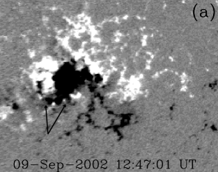
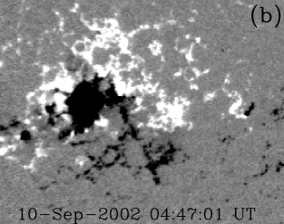
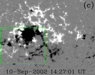
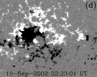
Figure 1.: Magnetic field evolution seen in MDI line of sight magnetograms during September 9 and 10, 2002. All images have been rotated to solar Sun center and saturated above (below) 300 G (-300 G). Notice that the field intensity in the negative spot is such that saturation is very clear in MDI data in Figure fig:MDI-HXR-sst. The arrows in panel (a) point to a chain of small bipoles located in the moat region surrounding the spot. The green box in panel (c) represents the field of view of the Figure fig:MDI-HXR-sst.fig:field-evolution

Adjacent to AR 10105, on its west, there is a dispersed bipolar facular region and a new AR to its SE (AR 10108, see Figure fig:field-evolutiona). Vigorous moving magnetic feature (MMF, see HarveyHarvey:1973) activity is seen (compare Figure fig:field-evolutiona to Figure fig:field-evolutionb and see the movie mag-field-evol.mpg that accompanies this paper) around the big leading spot and a moat boundary is visible in Figure fig:field-evolutiona mainly in a E-SE segment, where magnetic field aggregates at what appears the confluence of three supergranular cells. In particular, we have indicated within arrows in Figure fig:field-evolutiona a chain of small bipoles. Though this image is affected by projection effects, these bipolar regions persist in MDI magnetograms. Figure fig:field-evolutionb shows that the eastern negative polarity of the eastermost bipole rotates counter-clockwise around the positive one. This motion should increase the magnetic field shear in the region and, at the same time, favour the interaction with nearby bipoles in the MMFs to its north. Figure fig:field-evolutionc (see a zoom of this image in Figure fig:MDI-HXR-sst) shows the magnetic field at 14:27 UT on September 10, this is the closest in time magnetogram to the flare occurrence at 14:52 UT. In this magnetogram the negative polarity to the east (which is along the moat boundary) has decreased in size as flux cancellation proceeds with the positive bipole polarity. Along this period, flux cancellation also proceeds between this positive polarity and the nearby negative polarity of the bipole to the west. Finally, this small bipole is hardly observable by the end of the day (see Figure fig:field-evolutiond). The magnetic field evolution just discussed lets us infer the origin of the flare eruption and the location of the pre-reconnected set of loops and the reconnected loops of which only one is visible in the XR and EUV data (see Figure fig:MDI-HXR-sst and Section fig:MDI-HXR-sst).

2.3 Time profiles in radio and X-rays

sec:profiles

Figure 2.: Radio data at selected frequencies. The vertical bar on the 2.695 GHz plot indicates the short pulse. We include also 75–300 keV HXR from RHESSI and 1-8 Å SXR from GOES.fig:profiles

The time profiles are shown in Fig fig:profiles. The flare appears as a single impulsive peak in GOES data with a start at around 14:50 UT, peak time at 14:56 UT and a total duration of about 20 minutes. The soft-X rays (SXR) emission has a maximum flux $2.9\times 10^{-5}\ \mathrm{Wm}^{-2}$ (M2.9). We have derived a temperature $T_{goes}=14.4$ MK and emission measure $EM_{goes}=3.4\times 10^{48}\ \mathrm{cm}^{-3}$ using the Chianti 6.0.1 Coronal Model, during the HXR impulsive peak interval (14:52:50 - 14:53:00).

The impulsive phase is clearly visible at all radio frequencies covering almost two decades from 1 to 200 GHz, starting at approximately 14:52:30 UT. A short pulse is observed at the beginning of the event between 14:52:50 and 14:53 UT (indicated by a vertical bar on the 2.695 GHz panel) with a flux in excess of the main emission well defined between 1.415 and 4.995 GHz, above this range it is hardly distinguishable. The short duration and the narrow spectrum of this pulse reminds us of a similar one that also occurred during the rising phase of an event (SOL2002-08-30T13:28, GimenezdeCastroetal:2006). At 212 GHz, the flux density time profile is composed of a single peak, with maximum at 14:53:20 UT with a total duration of around 2 minutes. There is no clear evidence of an extended phase like in Luthietal:2004a and Trottetetal:2011. Besides, the HXR emission above 50 keV ends around the peak time of the radio emission, although the start time of both are similar, below 30 keV the emission extends longer. We note that this is one of the weakest GOES events that has a clear submillimeter counterpart. Indeed, as a comparison, the flare SOL2002-08-30T13:28 (X1.5) had a 212 GHz peak density flux of 150 s.f.u. [Giménez de Castro et al. (2009)]

We observe a frequency dependent time delay in the radio data, which in the four second integrated HXR data is not evident. Normalized time profiles integrated in one second bins are shown in Figure fig:delays (top) at each frequency with different colours. This figure gives the impression that each different frequency starts at slightly different times. To further investigate this, we analyzed the rising times at different frequencies. Since the start time is subjected to big uncertainties, we compared the time elapsed between a reference time and the time at which the emission reaches a certain normalized flux density. Moreover, we find more accurate to measure delays during the rising phase than during the, almost flat, maximum. We used two different normalized levels, 10% and 50%. For each frequency $\nu$ we found $t_{10}(\nu)$ and $t_{50}(\nu)$, the times when the flux density reaches the 10% and 50% relative level respectively. The reference is the 75–300 keV emission, with $t_{10}^{*}$ and $t_{50}^{*}$ defined when the HXR flux is 10% and 50% of the peak flux respectively. Delays are then defined as $\Delta_{10}(\nu)=t_{10}(\nu)-t_{10}^{*}$ and $\Delta_{50}(\nu)=t_{50}(\nu)-t_{50}^{*}$. To some extent $t_{10}^{*}$ and $t_{50}^{*}$ are arbitrarily defined, but in doing so we simultaneously have an indication of the relation between radio and HXR. Delays are determined with 0.5 s accuracy, derived from the worst time resolution we have in the radio data. The result is shown in Figure fig:delays (bottom). Above 10 GHz there is a continuous shift, which is, within the uncertainties, independent of the level (10% or 50%). This is qualitatively observed in the time profiles (Fig. fig:delays, top). Previous works have shown that millimeter/submillimeter emission is delayed from microwaves (see e.g. Limetal:1992,Trottetetal:2002, Luthietal:2004a), but this is the first time to our knowledge that a spectrum of the delay is presented. Below 7 GHz the presence of the short pulse distorts this trend.

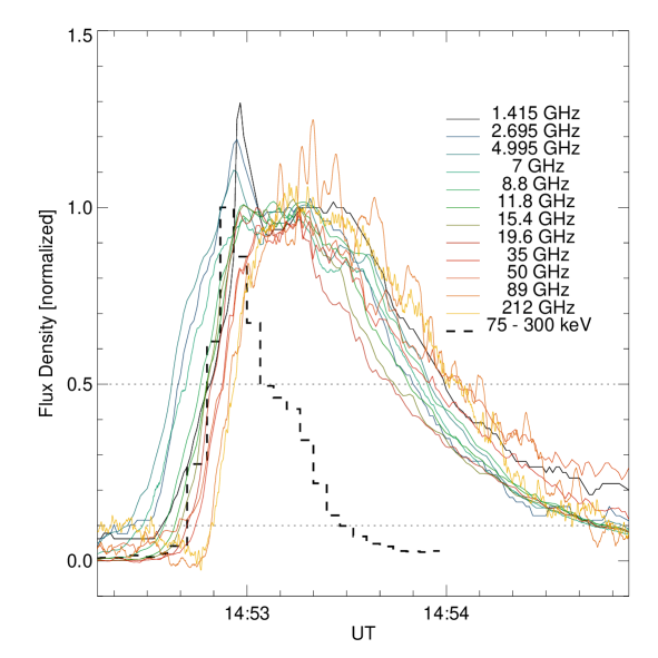
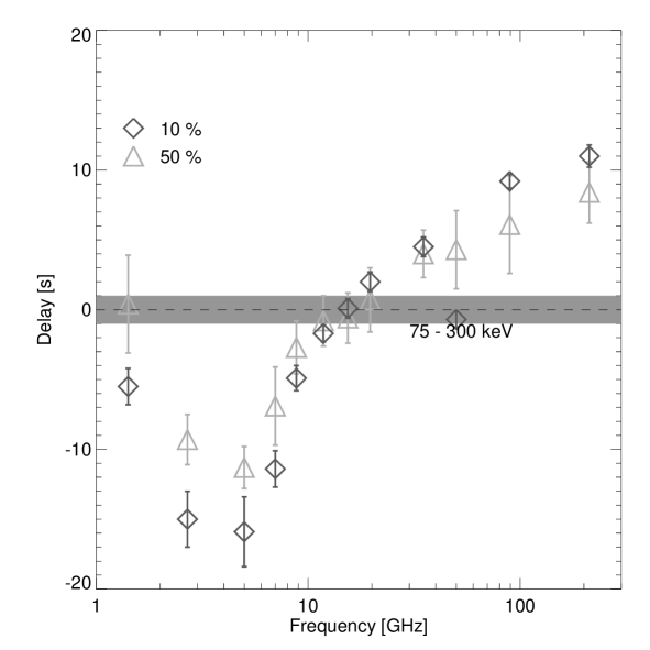
Figure 3.: Top: normalized flux densities from 1.415 to 212 GHz. Normalization fluxes are taken in the interval 14:5310 – 14:5330 UT. The dashed curve is the normalized 75–300 keV flux. Dotted horizontal lines, represent 10% and 50% levels. Bottom: Measured delays between radio and HXR. The horizontal gray band represents the uncertainty at 75–300 keV rising levels.fig:delays

2.4 X-Ray imaging and radio-source positions

sec:images

We produced X-ray images using RHESSI data. These images are constructed with the PIXON algorithm [Hurford et al. (2002)] with an accumulation time of four seconds (from 14:52:52 UT to 14:52:56 UT) for lower energy bands (below 80 keV), and twelve seconds (from 14:52:52 UT to 14:53:04 UT) for higher energy bands (above 100 keV). We used collimators 1–6 and a pixel size of 0.5^′′. We considered the following energy bands: 12–25 keV, 40–80 keV, 100–250 keV, 150–300 keV and 250–300 keV. The images show two sources clearly defined (see Fig. fig:MDI-HXR-sst). There is a loop or arcade connecting the two footpoints visible in the 12-25 keV energy band image (see Fig. fig:MDI-HXR-sst).

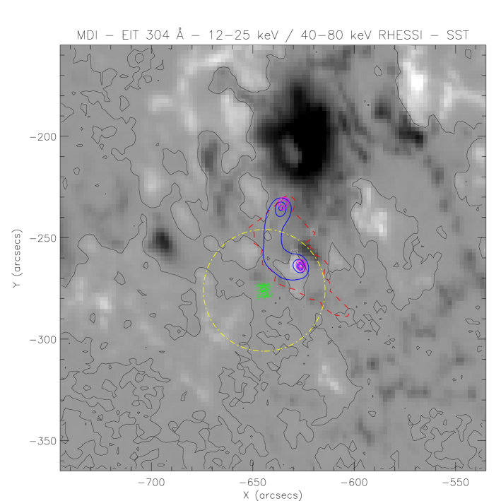
Figure 4.: MDI magnetogram closest in time to the event. The black lines denote magnetic polarity inversion lines. Blue contours are RHESSI 12–25 keV for the interval 14:52:52 to 14:52:56 UT, magenta lines are RHESSI 40–80 keV contour levels at 20%, 50% and 80% of the image maximum for the same time interval. A contour corresponding to 60% of the maximum intensity of the closest in time EIT image in 304 Å is also shown (red dashed contour). Green points indicate the centroid positions of the submillimeter emission from 14:52:40 to 14:54:40 UT (impulsive peak in radio) averaged every 0.4 s. The yellow dot–dashed circle denotes the absolute uncertainty in the determination of the radio–source positions ($\sim$30^′′), mainly limited by pointing accuracy.fig:MDI-HXR-sst

Fig. fig:MDI-HXR-sst shows the magnetogram closest in time ($\sim$14:27 UT) to the flare overlaid by RHESSI contours in the 12–25 (blue contours) and 40–80 (magenta contours) keV energy bands. Also included is a 60% of the maximum intensity contour of the closest in time 304 Å EIT image (red lines). Black thin contours correspond to the magnetic polarity inversion line, i.e. they separate positive from negative line of sight magnetic field. It is evident that both RHESSI footpoints overlay opposite sign polarities, with one of them located on the positive polarity, the evolution of which we discussed in Section sec:photosphere, and the other one on the negative polarity, north of it. Whithin the uncertainties of the reconstruction method, we did not observe any displacement in the HXR sources.

We determined the centroid of the sources emitting at 212 GHz every 40 ms during the impulsive phase of the event, assuming that the source size is small compared to the SST beam sizes (For a review of the multi–beam method see GimenezdeCastroetal:1999). At the same time, we corrected the flux density for mispointing. We note that since beam sizes are of the order of arcminutes, when they are not aligned with the emitting source the flux obtained from a single beam may be wrong.

In Figure fig:MDI-HXR-sst we have superimposed the positions of the 212 GHz burst emission centroids averaged every 0.4 s. They seem to be separated by 25^′′ from one of the HXR footpoints. The dot–dashed yellow circle represents the absolute uncertainty in the determination of the radio source position ($\sim$30”); this uncertainty is mainly due to the radiotelescope pointing accuracy. Because of this large absolute uncertainty, it is not possible to determine where the submillimeter source is located inside the loop, at the footpoints or at the loop top. The two X-ray sources in the flare seem to be associated with the bright ultraviolet enhancement seen by EIT encircling them. This brightening would correspond to an upper chromospheric loop also traced by the lowest energy RHESSI isocontours. Timing analysis does not reveal a displacement of the 212 GHz emission centroids in a privileged direction during the impulsive phase of the event. We can infer the compactness of the submillimeter source or sources because of the low level of spread, lower than 10^′′.

3 Spectral Analysis

sec:analysis

Figure 5.: Radio spectra ad selected times. The data, integrated in 1 s bins, are represented with their error bars. Dashed curves correspond to the low frequency fitting and dot-dashed curves to the high frequencies fitting. Continuous lines represent the total solution (low frequency + high frequency). fig:rspec-fit

Figure fig:rspec-fit shows integrated radio spectra at selected one second time intervals. The existence of composed spectra is evident after 14:52:50 UT. We distinguish two components that we call the low frequency and high frequency components. The low frequency one has a peak frequency around 10 GHz, while the high frequency is maximum at around 35 GHz. Because only the high frequency component shows clearly its optically thin part, we have used frequencies 50, 89.4 and 212 GHz to compute the spectral index $\alpha_{hf}$ along the event. Figure fig:delta bottom shows $\alpha_{hf}$ in function of time together with error bars. During the maximum of the event the spectral index remains stable, but at the beginning and the end a softening is observed, i.e. the index has an SHS behaviour. To get insight into the characteristics of electron populations that produced this emission, we have fitted the data to two homogeneous gyrosynchrotron sources using the traditional Ramaty:1969 procedure. The suprathermal electron distributions are represented by a power law with electron indices $\delta_{l\!f}$ and $\delta_{h\!f}$ for the low frequency and high frequency sources respectively. At each time interval, a model was fitted to the low frequency and another model to the high frequency, the sum of both was compared to the data until the best solution was obtained. In general we fixed the source size, the magnetic intensity, medium density and the electron energy cutoffs (see Table tbl:parametros). We allowed changes only in the electron indices $\delta_{l\!f}$, $\delta_{h\!f}$ and the total number of accelerated electrons. The fittings are shown in the Figure fig:rspec-fit. It is evident that below 9 GHz the fittings are rather poor, which is an indication that the source is not totally homogeneous [Klein, Trottet, and Magun (1986)], nonetheless we may be confident on the electron index and number, which depend on the optically thin part, and on the magnetic field which is defined by the peak frequency. Moreover, the good agreement with similar parameters derived from HXR is another indication of the goodness of the fittings (see below).

	Low Frequency	High Frequency
Parameter	Component	Component	Unit
Mag. Field	380	2000	G
Diameter	18	5	arc sec
Height	$10^{9}$	$10^{8}$	cm
Low En. Cutoff	20	20	keV
High En. Cutoff	10	10	MeV
Maximum Total Number of $e^{-}$	$4.7\times 10^{37}$	$7.6\times 10^{34}$

Table 1.: Fixed parameters used to fit the spectral data and maximum total electron number derived from the computations.tbl:parametros

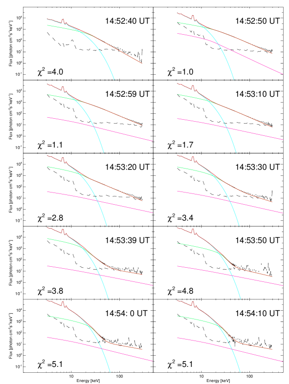
Figure 6.: HXR spectra at selected interval times. Data are integrated in 4 s bins and represented with error bars. Blue curves represent the thermal solution, green curves are the broken power law solution and red curves are the total solution (Thernal+broken power law). Magenta curves represent the expected emission from the relativistic electrons used to fit the radio high frequency component. Dashed curves are the background.fig:xspec-fit

HXR spectra were taken from 14:52:00UT to 14:54:00UT in 4 second intervals, using front detectors 1, 3, 4, 5, 6, 8 and 9, for energies between 3 and 290 keV. We excluded the time bin when there was a change in attenuator state, from 0 to 1. Due to the high flare activity during this RHESSI observation interval, we selected the background emission from the subsequent night period (15:18:48 – 15:22:12 UT). Figure fig:xspec-fit shows the photon flux spectra at selected time intervals along with the fitting used to calibrate the data. Using standard OSPEX procedures we applied a model of a thermal source, including continuum and lines, and a double power law. We found significant counts up to 300 keV, during peak time (14:52:59 UT). The thermal component is well represented by an isothermal source with a mean temperature $T_{hsi}=20.7$ MK and emission meassure $EM_{hsi}=1.2\times 10^{48}\ \mbox{cm}^{-3}$ during the HXR impulsive peak interval (14:52:50 - 14:53:00). The break energy remains always below 80 keV, and the electron index below it is always harder than the index above. The later was used to compare with radio data because electrons with energies $<100$ keV affect the gyroemission only in the optically thick part of the spectrum [White et al. (2011)] which we did not try to fit as noted before. We also have to take into account that HXR emission depends on the electron flux, therefore for non relativistic particles we should add 0.5 to $\delta_{X}$ to compare with radio [Holman et al. (2011)], and, since the HXR spectra are computed below 300 keV, we should compare $\delta_{X}$ with $\delta_{l\!f}$, because relativistic electrons are needed to produce gyrosynchrotron emission for frequencies above 50 GHz. In the bottom panel of Figure fig:delta we can see the evolution of electron indices. We observe that $\delta_{X}$ (dot-dashed curve) remains stable at the beginning and increases at the end. The low frequency index $\delta_{l\!f}$ remains stable until 14:53:25 UT and is comparable to $\delta_{X}$, then a sudden change takes place making it harder. On the other hand, the high frequency index (continuous line) $\delta_{h\!f}$ is much harder than $\delta_{l\!f}$ and $\delta_{X}$ as it was observed in previous works (see e.g. GimenezdeCastroetal:2009, Trottetetal:1998) and it evolves in the same way as the spectral index $\alpha_{hf}$.

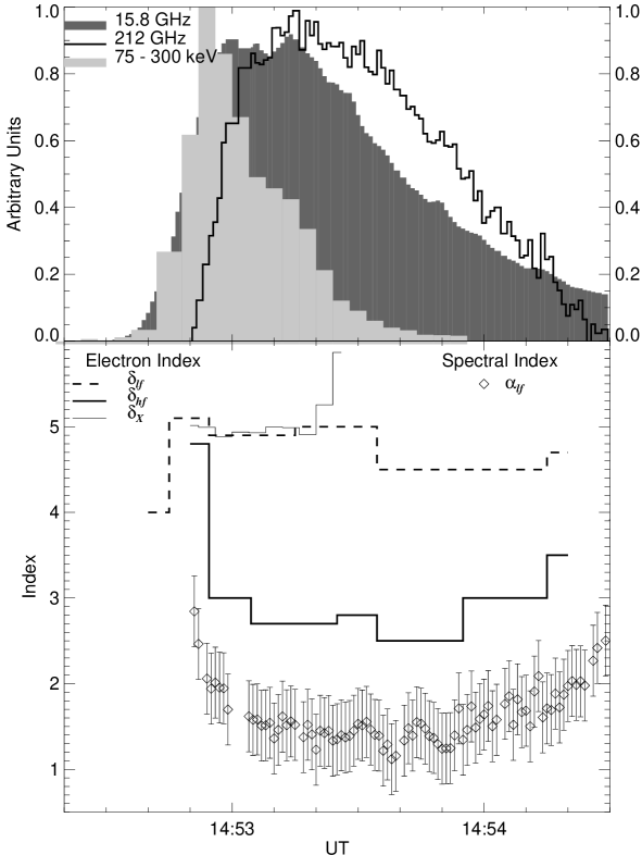
Figure 7.: Top panel: time profiles at 15.8 GHz (dark gray), 75–300 keV (light gray) and 212 GHz (continuous line). The bottom panel shows the time evolution of the electron indices together with the values and error bars of the high frequency optically thin spectral index $\alpha_{h\!f}$. fig:delta

4 Discussion

sec:discusion

The optically thin emission above 50 GHz is produced by relativistic particles, while the optically thick emission at microwaves and the HXR observed by RHESSI are emitted by mildly relativistic particles. We roughly divide the analysis in these two energy bands.

4.1 Dynamics of mildly relativistic electrons

sec:mild-relativistic

In order to understand the dynamics of the mildly relativistic electrons we compare the HXR emission, which it was observed up to 300 keV with the low frequency radio data. The comparison of the temporal evolution of both sets of data (see Figures fig:profiles and fig:delta) supports the existence of trapped electrons because: 1) the duration of the impulsive phase in HXR is shorter than in radio and 2) the peak time in HXR occurs before the radio peak, even at low frequencies. Therefore, the HXR time profile is not necessarily the representation of the injected electrons, since there are transport effects along the loop, or at least, HXR may represent the injected electrons that precipitate directly, without being subject to trapping.

We can use the spectral analysis to derive the rate of the injected electrons in the emitting area in function of time. To do so, we write a simplified continuity equation that depends only on time, since we are not interested on how the electron distribution changes in terms of energy, pitch angle, or depth. In this simplified model, we are interested only in the total instantaneous number of electrons, $N(t)$, inside the magnetic loop, incremented by a source, $Q(t)$, from the acceleration site and decremented by the precipitated electrons, $P(t)$. Therefore, the continuity equation should be

$$\frac{dN(t)}{dt}=Q(t)-P(t)\ .\ilabel{eq:cont}$$ (1)

Integrating the above equation in the interval $(t_{i},t_{i+1})$ (with $i=0,1,2\dots$) and solving for $Q(t_{i})$ yields

$$Q(t_{i})\Delta t_{i+1}=N(t_{i+1})-N(t_{i})+P(t_{i})\Delta t_{i+1}\ ,\ilabel{eq:injection}$$ (2)

with $\Delta t_{i+1}=t_{i+1}-t_{i}$. Since we are comparing $<300$ keV emission with gyrosynchrotron, we can identify the instantaneous number of electrons inside the loop $N(t)$ with the trapped particles emitting the lower frequency component. On the other hand, the particles leaving the volume $P(t)$ produce the HXR emission observed by RHESSI. In our picture, the low frequency component is produced all along a loop with a length of $10^{9}$ cm, while the HXR emission is produced in a narrow slab (see e.g. Holmanetal:2011) with a very small surface (see Figure fig:MDI-HXR-sst); therefore, we can neglect the gyroemission produced within this small volume. Furthermore, no change would be appreciated if one includes the particles responsible for the high frequency component since they are two orders of magnitude less than those that produce the low frequency component. (See Table tbl:parametros)

We divided the event in 10 second intervals and assumed that within these intervals the conditions do not change. The computation of Equation eq:injection is straightforward and the result is presented in Figure fig:injection. Since $>100$ keV data have good S/N ratio only between 14:52:50 UT and 14:53:30 UT, (see Figure fig:xspec-fit) the analysis is restricted to this interval, although is clear from the time profiles that there are emitting particles before and after. We observe a continuous injection with two peaks, one at the beginning and the second during the decay of the impulsive phase. To verify our results, we sum the precipitated electrons, $\sum_{i}P(t_{i})\Delta t=3.4\times 10^{37}$, and we compare this number with the maximum number of electrons existing instantaneously inside the loop, $\max[N(t_{i})]=4.7\times 10^{37}$. The difference between these two numbers maybe due to the fact that we are limited to the time interval in which the HXR data are statistically meaningful; therefore, we cannot track the precipitation until the end of the gyrosynchrotron emission.

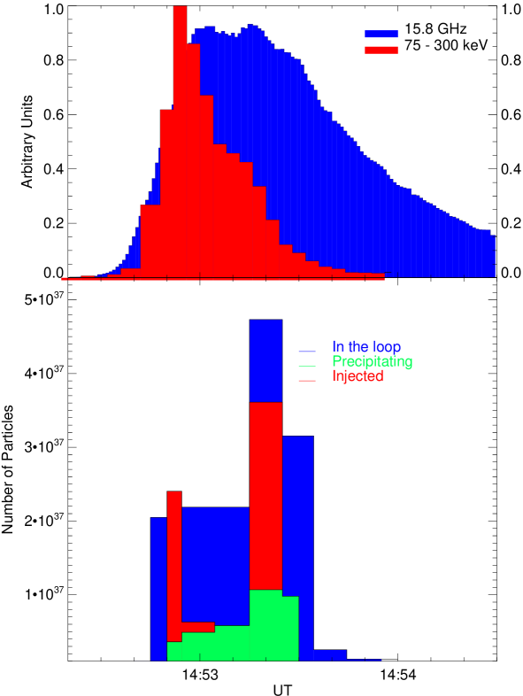
Figure 8.: Top: time profiles at 15.4 (blue) and 75–300 keV (red). Bottom: the precipitated electrons $P(t)\Delta t$ (green); the instantaneous number of electrons, $N(t)$ (blue), and the injected electrons $Q(t)\Delta t$ (red).fig:injection

We observe that changes in $\delta_{l\!f}$ (Fig. fig:delta) can be related to the injections occurred at around 14:52:51 UT and 14:53:15 UT (Figure fig:injection). The electron index $\delta_{X}$ lies around 5, as $\delta_{l\!f}$ for the same period, although, it increases slowly until 14:53:20 UT when it suddenly softens by around 0.5. The difference in time evolution of $\delta_{X}$ and $\delta_{l\!f}$ is an indication that the softening of the former is a consequence of the trapping. Since $\delta_{l\!f}$ has two constant values, we conclude that it is not affected by the medium. In the above analysis we rely upon the parameters derived from the radio and HXR data fittings. Although we do not claim that the obtained solutions are unique, the fact that two independent fittings give very comparable results, give us confidence on them.

The progressive delay of the radio emission observed in Figure fig:delays must be interpreted differently depending on the frequency range. Between 1 and 5 GHz, the short pulse dominates the emission during the rising phase; therefore, its contribution should be removed to asses the delay of the main emission. This may lead to ambiguous results, hence, we preferred not to analyze delays in this range. In the range between 9 and 30 GHz lies the peak frequency, i.e. the optical opacity $\tau$ is approximately 1, hence, the gyrosynchrotron self absorption is critical. The peak frequency ($\tau\simeq 1$) of the low frequency component shifts from approximately 7 GHz to 15 GHz from 14:52:40 UT to the peak time around 14:5259 UT (Fig. fig:rspec-fit). Since there is no change in the magnetic field, this can be interpreted by the accumulation of accelerated electrons inside the loop due to the trapping that increases its density, which is the dominant factor of the self-absorption mechanism. The shift makes the low frequencies more absorbed and thus increases the relative importance of higher frequencies. Therefore, even with a rather constant $\delta_{l\!f}$ (Fig. fig:delta) the progressive delay should be observed. In our fittings at 14:52:40 UT we have $\tau(\nu=7\ \mbox{GHz})=0.7$ and $\tau(\nu=10\ \mbox{GHz})=0.15$. Later on, during peak time $\tau(\nu=7\ \mbox{GHz})=60$ and $\tau(\nu=10\ \mbox{GHz})=3.7$. We note that the emission is proportional to $1-e^{-\tau}$, hence, we have a relative amplification of $(1-e^{-60})/(1-e^{-0.7})\simeq 1.4$ at 7 GHz, while it is $(1-e^{-3.7})/(1-e^{-0.15})\simeq 7.5$ at 10 GHz. The relative amplification changes the rate at which the emission rises and, therefore, the time when the signal reaches a certain level with respect to its maximum.

4.2 Relativistic Electrons

sec:relativistic

The centroid position of the emitting source at 212 GHz remains quite stable during the flare which may imply that the source is compact. Moreover, it is placed 25^′′ far from one of the HXR footpoints (Figure fig:MDI-HXR-sst). A similar result was obtained by Trottetetal:2008 for the SOL2003-10-28T11:10 flare; during the impulsive phase (interval B in their work) the centroid positions of the 210 GHz emission lie at approximately 10^′′ from the center of one of the HXR footpoints (250–300 keV), but are coincident with the location of precipitating high energy protons with energies above 30 MeV seen in $\gamma$-ray imaging of the 2.2 MeV line emission. Since for our work we do not have $\gamma$-ray imaging to compare with, we should be cautious because the uncertainty in position is of the order of the position shift.

Since we observe the optically thin part of the high frequency spectra, the obtained $\delta_{h\!f}$ is not affected by the medium and, within data uncertainties, it must be correct. On the other hand, we assumed a standard viewing angle $\theta=45^{\circ}$ which gives us a mean value of the magnetic field $B$ and total number of electrons $N$. Increasing (reducing) $\theta$ results in smaller (larger) $B$ and $N$. Although we cannot rightly evaluate $\theta$ with our data, we do not expect an extreme value for it since the AR is located not far from Sun center (E43). Furthermore we did consider an isotropic electron distribution. The total number of accelerated electrons is $8\times 10^{34}$ during peak time, and they should not produce enough bremsstrahlung flux to be detected by RHESSI detectors. We confirmed this by computing its HXR emission using the bremthick program (magenta curves in Figure fig:xspec-fit) which is orders of magnitude smaller than the mildly relativistic electron emission and remains below (except during one time interval) the background.

The spectral index of the high frequency component $\alpha_{hf}$ shows a SHS behaviour, but in this case we cannot conclude whether its origin comes from the acceleration mechanism or from the interaction with the medium as before. We tend to think that the former should be the cause, since these are relativistic particles and their interaction with the medium should be less effective. The emission must come from a compact region with a strong magnetic field and the electron index $\delta_{h\!f}$ should be harder than $\delta_{X}$ and $\delta_{l\!f}$, as is the case. These arguments support the evidence of the existence of a separated source where relativistic electrons are the responsible for the emission.

The progressive delay of the radio emission above 50 GHz (Figure fig:delays) can be interpreted considering the initial hardening of the spectral index $\alpha_{hf}$. If it is due to the acceleration mechanism that accelerates first the low energy particles and later the high energy particles, then, the progressive delay is a consequence.

5 Final Remarks

sec:fin

From our simple continuity model, we inferred the evolution of injected number of electrons, appearing as a continuous injection with two distinctive pulses separated by approximately 30 seconds. From the timing of those pulses, the first one produces the HXR and initiates the radio low frequency emission. The second pulse, while slightly stronger than the first, builds up into the radio emission but do not contributes to generate more HXR. This description suggests that the two injection might have different initial pitch angle distributions, because our fittings do not show magnetic field changes during the burst. The first injection might be formed by an electron beam aligned with the magnetic field direction, a fraction of the population is trapped by magnetic mirroring, while the other fraction enter the loss cone and precipitates, producing HXR. The second pulse should then be formed by a beam with a wider pitch angle distribution, or even isotropic, keeping most of the electrons trapped, producing radio emission, with little precipitation (no significant increase in HXR).

From our observations we conclude that the radio spectra cannot be explained by an homogeneous gyrosynchrotron source, therefore we adopted a model based on two homogeneous sources since it is the simplest hypothesis that fits reasonably the data. Although we don’t have images to support this assumption, it is plausible that it is the case. As shown by the magnetic field evolution discussed in Section 2.2, we can conclude that the flare originates by the interaction of magnetic loops anchored in the MMF polarities. Magnetic energy is probably increased in the configuration by shearing motions, in particular, the rotation of the negative polarity around the positive one. After magnetic reconnection occurs, two sets of reconnected loops should be present. In the example we have analyzed, we observe a set of loops in SXR (and also in EUV) with two HXR footpoints. Considering our description in Section sec:photosphere, we speculate that the second set of reconnected loops (not visible) could be anchored in the higher magnetic field positive polarity located north of the northern HXR footpoint and the negative polarity that rotates around the positive bipole polarity. Such a set of reconnected loops would have a larger volume than the ones that are observed; therefore, considering that the same amount of energy is injected in both sets, the emission in the second one could be less intense and, then, not visible. This second magnetic structure is also suggested by the 25^′′ displacement of the emitting source at 212 GHz respect to one of the HXR footpoints (Figure fig:MDI-HXR-sst). While it has been shown that the reconnection of many different magnetic loops is more efficient to accelerate high energy electrons (see Trottetetal:2008 and references therein), we might conclude that this complex mechanism operates even in medium size events as the one we analyzed in this work.

Another possible scenario is a loop structure where the low frequency source represents the coronal part of the loop (with a lower effective magnetic field strength), and the high frequency source represents the low coronal or chromospheric footpoints of the loop (with a higher effective magnetic field strength). Melnikovetal:2011, using simulations of electron dynamics and gyrosynchrotron emission in a loop structure, demonstrated that two spectral components can be produced from one single loop, where mildly-relativistic electrons produce microwave emission in the loop, while relativistic electrons produce higher frequency (reaching sub-THz frequencies) emission from the footpoints.

Acknowledgements

CGGC is grateful to FAPESP (Proc. 2009/18386-7). CHM acknowledge financial support from the Argentinean grants UBACyT 20020100100733, PIP 2009-100766 (CONICET), and PICT 2007-1790 (ANPCyT). PJAS is grateful to FAPESP (Proc. 2008/09339-2) and to the European Commission (project HESPE FP7-2010-SPACE-1-263086). GDC and CHM are members of the Carrera del Investigador Científico (CONICET), CGGC is level 2 fellow of CNPq and Investigador Correspondiente (CONICET).

References

- Correia, Kaufmann, and Melnikov (1999) Correia, E., Kaufmann, P., Melnikov, V.: 1999, Itapetinga 7 GHz polarimeter. In: Bastian, T., Gopalswamy, N., Shibasaki, K. (eds.) Proc. of the Nobeyama Symposium, 263 – +.
- Cristiani et al. (2008) Cristiani, G., Giménez de Castro, C.G., Mandrini, C.H., Machado, M.E., Silva, I.D.B.E., Kaufmann, P., Rovira, M.G.: 2008, A solar burst with a spectral component observed only above 100 GHz during an M class flare. A&A 492, 215 – 222. doi:10.1051/0004-6361:200810367.
- Delaboudiniere et al. (1995) Delaboudiniere, J.-P., Artzner, G.E., Brunaud, J., Gabriel, A.H., Hochedez, J.F., Millier, F., Song, X.Y., Au, B., Dere, K.P., Howard, R.A., Kreplin, R., Michels, D.J., Moses, J.D., Defise, J.M., Jamar, C., Rochus, P., Chauvineau, J.P., Marioge, J.P., Catura, R.C., Lemen, J.R., Shing, L., Stern, R.A., Gurman, J.B., Neupert, W.M., Maucherat, A., Clette, F., Cugnon, P., van Dessel, E.L.: 1995, EIT: Extreme-Ultraviolet Imaging Telescope for the SOHO Mission. Sol. Phys. 162, 291 – 312.
- Fleishman and Kontar (2010) Fleishman, G.D., Kontar, E.P.: 2010, Sub-Thz Radiation Mechanisms in Solar Flares. ApJ 709, L127 – L132. doi:10.1088/2041-8205/709/2/L127.
- Giménez de Castro et al. (1999) Giménez de Castro, C.G., Raulin, J.-P., Makhmutov, V.S., Kaufmann, P., Costa, J.E.R.: 1999, Instantaneous positions of microwave solar bursts: Properties and validity of the multiple beam observations. A&AS 140, 373 – 382.
- Giménez de Castro et al. (2006) Giménez de Castro, C.G., Costa, J.E.R., Silva, A.V.R., Simões, P.J.A., Correia, E., Magun, A.: 2006, A very narrow gyrosynchrotron spectrum during a solar flare. A&A 457, 693 – 697. doi:10.1051/0004-6361:20054438.
- Giménez de Castro et al. (2009) Giménez de Castro, C.G., Trottet, G., Silva-Valio, A., Krucker, S., Costa, J.E.R., Kaufmann, P., Correia, E., Levato, H.: 2009, Submillimeter and X-ray observations of an X class flare. A&A 507, 433 – 439. doi:10.1051/0004-6361/200912028.
- Guidice et al. (1981) Guidice, D.A., Cliver, E.W., Barron, W.R., Kahler, S.: 1981, The Air Force RSTN System. In: Bulletin of the American Astronomical Society, Bulletin of the American Astronomical Society 13, 553 – +.
- Harvey and Harvey (1973) Harvey, K., Harvey, J.: 1973, Observations of Moving Magnetic Features near Sunspots. Sol. Phys. 28, 61 – 71. doi:10.1007/BF00152912.
- Holman et al. (2011) Holman, G.D., Aschwanden, M.J., Aurass, H., Battaglia, M., Grigis, P.C., Kontar, E.P., Liu, W., Saint-Hilaire, P., Zharkova, V.V.: 2011, Implications of X-ray Observations for Electron Acceleration and Propagation in Solar Flares. Space Sci. Rev., 260 – +. doi:10.1007/s11214-010-9680-9.
- Hurford et al. (2002) Hurford, G.J., Schmahl, E.J., Schwartz, R.A., Conway, A.J., Aschwanden, M.J., Csillaghy, A., Dennis, B.R., Johns-Krull, C., Krucker, S., Lin, R.P., McTiernan, J., Metcalf, T.R., Sato, J., Smith, D.M.: 2002, The RHESSI Imaging Concept. Sol. Phys. 210, 61 – 86. doi:10.1023/A:1022436213688.
- Kaufmann (1971) Kaufmann, P.: 1971, The New Itapetinga Radio Observatory, from Mackenzaie University, São Paulo, Brazil. Sol. Phys. 18, 336.
- Kaufmann and Raulin (2006) Kaufmann, P., Raulin, J.-P.: 2006, Can microbunch instability on solar flare accelerated electron beams account for bright broadband coherent synchrotron microwaves? Physics of Plasmas 13, 701 – 704. doi:10.1063/1.2244526.
- Kaufmann et al. (2004) Kaufmann, P., Raulin, J.-P., de Castro, C.G.G., Levato, H., Gary, D.E., Costa, J.E.R., Marun, A., Pereyra, P., Silva, A.V.R., Correia, E.: 2004, A New Solar Burst Spectral Component Emitting Only in the Terahertz Range. ApJ 603, L121 – L124.
- Kaufmann et al. (2008) Kaufmann, P., Levato, H., Cassiano, M.M., Correia, E., Costa, J.E.R., Giménez de Castro, C.G., Godoy, R., Kingsley, R.K., Kingsley, J.S., Kudaka, A.S., Marcon, R., Martin, R., Marun, A., Melo, A.M., Pereyra, P., Raulin, J.-P., Rose, T., Silva Valio, A., Walber, A., Wallace, P., Yakubovich, A., Zakia, M.B.: 2008, New telescopes for ground-based solar observations at submillimeter and mid-infrared. In: Society of Photo-Optical Instrumentation Engineers (SPIE) Conference Series, Society of Photo-Optical Instrumentation Engineers (SPIE) Conference Series 7012. doi:10.1117/12.788889.
- Klein, Trottet, and Magun (1986) Klein, K.-L., Trottet, G., Magun, A.: 1986, Microwave diagnostics of energetic electrons in flares. Sol. Phys. 104, 243 – 252.
- Lüthi, Lüdi, and Magun (2004) Lüthi, T., Lüdi, A., Magun, A.: 2004, Determination of the location and effective angular size of solar flares with a 210 GHz multibeam radiometer. A&A 420, 361 – 370.
- Lüthi, Magun, and Miller (2004) Lüthi, T., Magun, A., Miller, M.: 2004, First observation of a solar X-class flare in the submillimeter range with KOSMA. A&A 415, 1123 – 1132.
- Lim et al. (1992) Lim, J., White, S.M., Kundu, M.R., Gary, D.E.: 1992, The high-frequency characteristics of solar radio bursts. Sol. Phys. 140, 343 – 368. doi:10.1007/BF00146317.
- Lin and et al. (2002) Lin, R.P., et al.: 2002, The Reuven Ramaty High-Energy Solar Spectroscopic Imager (RHESSI). Sol. Phys. 210, 3 – 32.
- Melnikov, Costa, and Simões (2012) Melnikov, V., Costa, J.E.R., Simões, P.J.A.: 2012, Sub-THz flare emission: an evidence for relativistic electron beams in the dense chromosphere. Sol. Phys.. In preparation.
- Ramaty (1969) Ramaty, R.: 1969, Gyrosynchrotron Emission and Absorption in a Magnetoactive Plasma. ApJ 158, 753 – +.
- Ramaty et al. (1994) Ramaty, R., Schwartz, R.A., Enome, S., Nakajima, H.: 1994, Gamma-ray and millimeter-wave emissions from the 1991 June X-class solar flares. ApJ 436, 941 – 949.
- Scherrer et al. (1995) Scherrer, P.H., Bogart, R.S., Bush, R.I., Hoeksema, J.T., Kosovichev, A.G., Schou, J., Rosenberg, W., Springer, L., Tarbell, T.D., Title, A., Wolfson, C.J., Zayer, I., MDI Engineering Team: 1995, The Solar Oscillations Investigation - Michelson Doppler Imager. Sol. Phys. 162, 129 – 188.
- Silva et al. (2007) Silva, A.V.R., Share, G.H., Murphy, R.J., Costa, J.E.R., de Castro, C.G.G., Raulin, J.-P., Kaufmann, P.: 2007, Evidence that Synchrotron Emission from Nonthermal Electrons Produces the Increasing Submillimeter Spectral Component in Solar Flares. Sol. Phys. 245, 311 – 326. doi:10.1007/s11207-007-9044-0.
- Trottet et al. (1998) Trottet, G., Vilmer, N., Barat, C., Benz, A., Magun, A., Kuznetsov, A., Sunyaev, R., Terekhov, O.: 1998, A multiwavelength analysis of an electron-dominated gamma-ray event associated with a disk solar flare. A&A 334, 1099 – 1111.
- Trottet et al. (2002) Trottet, G., Raulin, J.-P., Kaufmann, P., Siarkowski, M., Klein, K.-L., Gary, D.E.: 2002, First detection of the impulsive and extended phases of a solar radio burst above 200 GHz. A&A 381, 694 – 702.
- Trottet et al. (2008) Trottet, G., Krucker, S., Lüthi, T., Magun, A.: 2008, Radio Submillimeter and -Ray Observations of the 2003 October 28 Solar Flare. ApJ 678, 509 – 514. doi:10.1086/528787.
- Trottet et al. (2011) Trottet, G., Raulin, J.-P., Giménez de Castro, C.G., Lüthi, T., Caspi, A., Mandrini, C., Luoni, M.L., Kaufmann, P.: 2011, Origin of the submillimeter radio emission during the time-extended phase of a solar flare. Sol. Phys.. submitted.
- White et al. (2011) White, S.M., Benz, A.O., Christe, S., Fárník, F., Kundu, M.R., Mann, G., Ning, Z., Raulin, J.-P., Silva-Válio, A.V.R., Saint-Hilaire, P., Vilmer, N., Warmuth, A.: 2011, The Relationship Between Solar Radio and Hard X-ray Emission. Space Sci. Rev., 263. doi:10.1007/s11214-010-9708-1.