VLBA monitoring of Mrk 421 at 15 GHz and 24 GHz during 2011

Abstract

Context. High-resolution radio observations are ideal for constraining the value of physical parameters in the inner regions of active-galactic-nucleus jets and complement results on multiwavelength (MWL) observations. This study is part of a wider multifrequency campaign targeting the nearby TeV blazar Markarian 421 (z=0.031), with observations in the sub-mm (SMA), optical/IR (GASP), UV/X-ray (Swift, RXTE, MAXI), and $\gamma$ rays (Fermi-LAT, MAGIC, VERITAS).

Aims. We investigate the jet’s morphology and any proper motions, and the time evolution of physical parameters such as flux densities and spectral index. The aim of our wider multifrequency campaign is to try to shed light on questions such as the nature of the radiating particles, the connection between the radio and $\gamma$-ray emission, the location of the emitting regions and the origin of the flux variability.

Methods. We consider data obtained with the Very Long Baseline Array (VLBA) over twelve epochs (one observation per month from January to December 2011) at 15 GHz and 24 GHz. We investigate the inner jet structure on parsec scales through the study of model-fit components for each epoch.

Results. The structure of Mrk 421 is dominated by a compact ($\sim$0.13 mas) and bright component, with a one-sided jet detected out to $\sim$10 mas. We identify 5-6 components in the jet that are consistent with being stationary during the 12-month period studied here. Measurements of the spectral index agree with those of other works: they are fairly flat in the core region and steepen along the jet length. Significant flux-density variations are detected for the core component.

Conclusions. From our results, we draw an overall scenario in which we estimate a viewing angle $2^{\circ}<\theta<5^{\circ}$ and a different jet velocity for the radio and the high-energy emission regions, such that the respective Doppler factors are $\delta_{r}\sim 3$ and $\delta_{\rm h.e.}\sim 14$.

1 Introduction

Table 1: Details of the observations.

Observation	MJD	Map peak		Beam		1$\sigma$ rms		Notes
date		(mJy/beam)		(mas $\times$ mas, ∘)		(mJy/beam)
		15 GHz	24 GHz	15 GHz	24 GHz	15 GHz	24 GHz
2011/01/14	55575	348	319	1.05 $\times$ 0.65, 15.3	0.79 $\times$ 0.47, 8.84	0.19	0.18	No MK, no NL
2011/02/25	55617	391	338	1.16 $\times$ 0.74, 14.4	0.64 $\times$ 0.39, $-$6.52	0.35	0.18	NL snowing
2011/03/29	55649	386	359	1.06 $\times$ 0.66, $-$5.37	0.65 $\times$ 0.39, $-$4.26	0.17	0.24	No HK
2011/04/25	55675	367	308	0.92 $\times$ 0.50, $-$3.79	0.61 $\times$ 0.34, $-$3.88	0.28	0.33	-
2011/05/31	55712	355	297	0.93 $\times$ 0.51, $-$5.56	0.64 $\times$ 0.35, $-$8.41	0.25	0.29	-
2011/06/29	55741	262	208	0.89 $\times$ 0.50, $-$7.17	0.56 $\times$ 0.32, $-$12.3	0.17	0.37	No LA
2011/07/28	55770	220	197	0.91 $\times$ 0.56, $-$0.89	0.60 $\times$ 0.37, $-$1.14	0.20	0.30	-
2011/08/29	55802	275	200	0.97 $\times$ 0.55, 0.26	0.63 $\times$ 0.35, $-$2.70	0.18	0.27	No HK
2011/09/28	55832	264	238	1.06 $\times$ 0.67, 16.2	0.72 $\times$ 0.47, 18.4	0.26	0.24	No MK
2011/10/29	55863	261	167	1.06 $\times$ 0.69, 0.09	0.73 $\times$ 0.44, $-$3.73	0.26	0.14	HK snowing
2011/11/28	55893	283	201	1.02 $\times$ 0.59, 18.0	0.70 $\times$ 0.42, 14.3	0.28	0.17	No PT, FD, MK
2011/12/23	55918	295	287	0.89 $\times$ 0.49, 1.82	0.61 $\times$ 0.35, $-$5.74	0.15	0.21	No HK

Figure 1: Images of Mrk 421 at 15 GHz (left panel) and 24 GHz (right panel). These two images were obtained by stacking all of the images of the twelve epochs, at the respective frequency. The restoring beam for the 15 GHz image is 0.9 mas$\times$0.55 mas and the peak flux density is 307.2 mJy/beam. For the 24 GHz image, the restoring beam is 0.6 mas$\times$0.35 mas and the peak is 251.9 mJy/beam. The first contour is 0.35 mJy/beam, which corresponds to three times the off-source noise level. Contour levels are drawn at ($-$1, 1, 1.4, 2, 2.8, 4…) in steps of $\sqrt{2}$.

Markarian 421 (R.A.=$11^{h}$ $04^{m}$ $27.313943^{s}$, Dec.=$+38^{\circ}$ 12′ 31.79906″, J2000) is one of the nearest ($z=0.031$) and brightest BL Lac objects in the sky. It was the first extragalactic source detected at TeV energies by the Cherenkov telescope at Whipple Observatory (Punch et al. 1992). The spectral energy distribution (SED) of this object, dominated by non-thermal emission, has two smooth broad components: one at lower energies, from radio band to the soft X-ray domain, and another at higher energies peaking at $\gamma$-ray energies (Abdo et al. 2011). The low-frequency peak is certainly due to synchrotron emission from relativistic electrons in the jet interacting with the magnetic field, whereas the high-frequency peak is probably due to the inverse Compton scattering of the same population of relativistic electrons with synchrotron low-energy photons (synchrotron-self-compton model, SSC, see Abdo et al. 2011; Tavecchio et al. 2001). In this framework, multiwavelength (MWL) coordinated campaigns are a fundamental tool for understanding the physical properties of the source, e.g. by studying variability, which is present at all frequencies, but particularly TeV energies where Gaidos et al. (1996) measured a doubling time of $\sim 15$ minutes. The accurate MWL study and SED modeling performed by Abdo et al. (2011) revealed some interesting results, such as the size of the emitting region $R$ and the magnetic field $B$, which in the context of the leptonic scenario they constrained to be $R\lesssim 10^{4}R_{g}$ and $B\sim$ 0.05 G. However, the details of the physical processes responsible for the observed emission are still poorly constrained. Because of the considerable variability and the broadband spectrum, multiwavelength long-term observations are required for a good comprehension of the emission mechanisms.

This study is part of a new multi-epoch and multi-instrument campaign, which also involves observations in the sub-mm (SMA), optical/IR (GASP), UV/X-ray (Swift, RXTE, MAXI), and $\gamma$ rays (Fermi-LAT, MAGIC, VERITAS), as well as at the cm wavelengths with low resolution observations (e.g. F-GAMMA, Medicina). The aim of this observational effort is to shed light on fundamental questions such as the nature of the radiating particles, the connection between the radio and $\gamma$-ray emission, the location of the emitting regions, and the origin of the flux variability. Very long baseline interferometry (VLBI) plays an important role in addressing these scientific questions because it is the only technique that can resolve (at least partially) the inner structure of the jet. Therefore, cross-correlation studies of Very Long Baseline Array (VLBA) data with data from other energy ranges (in particular $\gamma$ rays) can provide us with important information about the structure of the jet and the location of the blazar emission.

At radio frequencies, Mrk 421 clearly shows a one-sided jet structure aligned at a small angle with respect to the line of sight (Giroletti et al. 2006). In this work, we present new VLBA observations to study in detail the inner jet structure on parsec scales. We are able to investigate the evolution of shocks that arise in the jet, by means of the model-fitting technique. In earlier works (Piner et al. 1999; Piner & Edwards 2004), the jet components show only subluminal apparent motion, which seems to be a common characteristic of TeV blazars. Thanks to accurate measurements of changes on parsec scales, by the VLBA, we can find valid constraints on the geometry and kinematics of the jet.

This paper is structured as follows: in Section 2 we introduce the dataset, in Section 3 we report the results of this work (model fits, flux density variations, apparent speeds, jet sidedness, spectral index), and in Section 4 we discuss results giving our own interpretation in the astrophysical context. We used the following conventions for cosmological parameters: $H_{0}=70$ km sec^-1 Mpc^-1, $\Omega_{M}=0.25$ and $\Omega_{\Lambda}=0.75$, in a flat Universe. We defined the spectral index $\alpha$ such that $S_{\nu}\propto\nu^{\alpha}$.

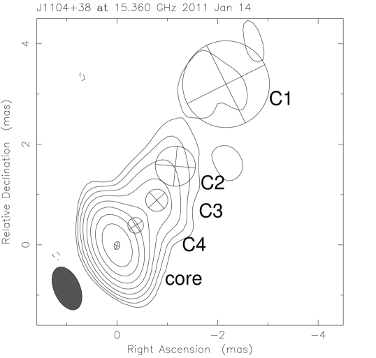
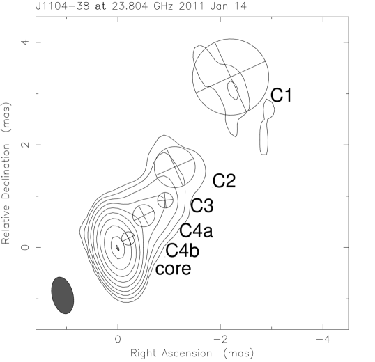
Figure 2: Images of Mrk 421 with model fit components for the first epoch at 15 GHz (left panel) and at 24 GHz (right panel). Levels are drawn at $(-1,1,2,4...)\times$ the lowest contour, that is at 1.0 mJy/beam for both images, in steps of 2. The restoring beam is shown in the bottom left corner; its size is given in Table 1.

2 Observations

We observed Mrk 421 throughout 2011 with the VLBA. The source was observed once per month, for a total of 12 epochs, at three frequencies: 15, 24, and 43 GHz. In this paper, we present the complete analysis of the whole 15 and 24 GHz datasets. We also observed, at regular intervals, three other sources (J0854+2006, J1310+3220, and J0927+3902) used as fringe finders and calibrators for the band pass, the instrumental (feed) polarization, and the electric-vector position angle. At each epoch, Mrk 421 was observed for nearly 40 minutes at each frequency, spread into several scans of about 3 minutes each, interspersed with calibrator sources in order to improve the (u,v)-coverage. Calibrators were observed for about 10 minutes each, generally spread into three scans of 3 minutes.

For calibration and fringe-fitting, we used the AIPS software package (Greisen 2003), and for image production the standard self-calibration procedures included in the DIFMAP software package (Shepherd 1997), which uses the CLEAN algorithm proposed by Högbom (1974). In some epochs, one or more antennas did not work properly because of technical problems; for a complete report (see Table 1).

3 Results

3.1 Images

We show in Fig. 1 two images of Mrk 421 at 15 and 24 GHz, which were produced by stacking all the images respectively at 15 and 24 GHz created with DIFMAP. The alignment of the images was checked by comparing the pixel position of the peak. In both images, we set the lowest contour equal to about three times the off-source residual rms noise level.

All the 12 images at each frequency show a similar structure, consisting of a well-defined and well-collimated one-sided jet structure emerging from a compact nuclear region (core-dominated source). This is the typical structure of a BL Lac object (Giroletti et al. 2004a). The jet extends for roughly 4.5 mas (2.67 pc), with a position angle (PA) of $\sim-35^{\circ}$ (measured from north through east). This morphology agrees with the results of other studies of similar angular resolution (Marscher 1999).

Since the morphology was very stable from epoch to epoch, the stacking did not smear any details of the structure. A sample couple of 15 and 24 GHz images is shown in Fig. 2.

3.2 Model fits

For each epoch, we used the model-fitting routine in DIFMAP to fit the visibility data of the source in the $(u,v)$ plane with either elliptical or circular Gaussian components. In this way, we were able to investigate in detail the inner jet structure and its evolution. For all epochs at 15 GHz, a good fit was obtained with five Gaussian components, while at 24 GHz we needed six components. At both frequencies, we identified the core with the brightest, innermost, and most compact feature. We label the other components C1, C2, C3, and C4, starting from the outermost (C1) to the innermost (C4). The higher angular resolution achieved at 24 GHz resolves the second innermost 15 GHz component (C4 located at $\sim$0.45 mas from the core) into two features (C4b at $\sim$0.3 mas and C4a $\sim$0.7 mas from the core) (see Fig. 2).

Thanks to the extremely fine time-sampling, we were able to make an attempt to identify the same component in each epoch. Overall, the components extend out to a region of about 5 mas. In this way, with a limited number of components, it was possible to analyze the proper motions and flux density levels at various times. From Fig. 3, we can clearly see that the data occupy well-defined regions in the radius vs. time plot, and that this behavior helps us to identify the individual components across epochs.

All details of the model fit analysis are shown in Table LABEL:gaussian. We calculated the uncertainties in the position (error bars in Fig. 3) using the ratio of the size of each component to the signal-to-noise ratio (S/N). In the case of very bright, compact components, the nominal error value is too small and replaced by a conservative value equal to 10% of the beam size (Orienti et al. 2011). On the other hand, when the calculated error is very large (i.e. comparable to the component radius, as in the case of a very extended component with a very low flux density), we replace it with a threshold value equal to the maximum value of the calculated errors for the same component at different epochs.

By comparing with Piner et al. (2010) and Piner & Edwards (2005), we can argue that the components C2, C3, C4a, and C4b of the present analysis quite likely correspond respectively to the components C5, C6, C7, and C8 of the aforementioned works. We also suggest that our component C1 corresponds to their component C4a. We will consider a more accurate identification of our components with those of previous analyses in a forthcoming paper, where the 43 GHz data analysis will also be presented.

Figure 3: Results of model-fit analysis. Circles and triangles refer, respectively, to positions of the Gaussian components at 15 and 24 GHz.

3.3 Flux density variability

Using the results of the model-fit technique, we analyzed the temporal evolution of the flux density for each component of the source. The brightest component represents the core; at 15 GHz, it has a mean value of around 350 mJy, which decreases along the jet until values of about 10 mJy. By comparing the flux density of each component at the various epochs, it emerges that there are no significant variations in the flux densities of the C1-C4 components. The flux density of each component remains roughly constant at various times within the uncertainties calculated; in any case, there is no indication of flaring activity. Any small variations may be artifacts brought about by our fitting procedures: for instance, the flux density of the inner components may be underestimated in some cases, because part of it was incorporated into the core component flux, or the flux density of the most extended features may be underestimated at epochs missing some short baseline data because of telescope failures. This is a remarkable result because it also allows us to identify components based on their flux density values and confirms our choice of components based on their positions.

In Fig. 4, we show the light curve for Mrk 421 during 2011 at 15 GHz (upper panel) and at 24 GHz (lower panel), considering the total flux density (squares) and the core flux density (triangles). The light curve reveals an interesting feature: in the second part of the year (starting at MJD $\sim$55700), we clearly note a decrease in the total flux density. From the complete flux-density analysis, we found that the core is the component responsible for the decrease, while the extended region does not display any significant variations. To further exclude calibration effects, we performed the same analysis on the three calibrators. In Fig. 4, we present the light curves of the calibrator J1310+3220 (diamonds) at 15 GHz (upper panel) and 24 GHz (lower panel). From this comparison, we clearly see that the trend of the light curves for the two sources is very different. We can assert that the flux density decrease observed for the core of Mrk 421 is a real feature. Error bars were calculated by considering a calibration error of about $10\%$ of the flux density and a statistical error equal to three times the map rms noise.

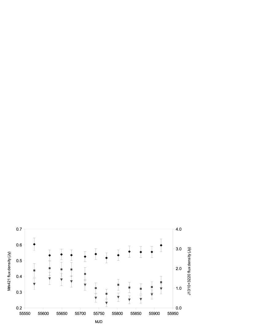
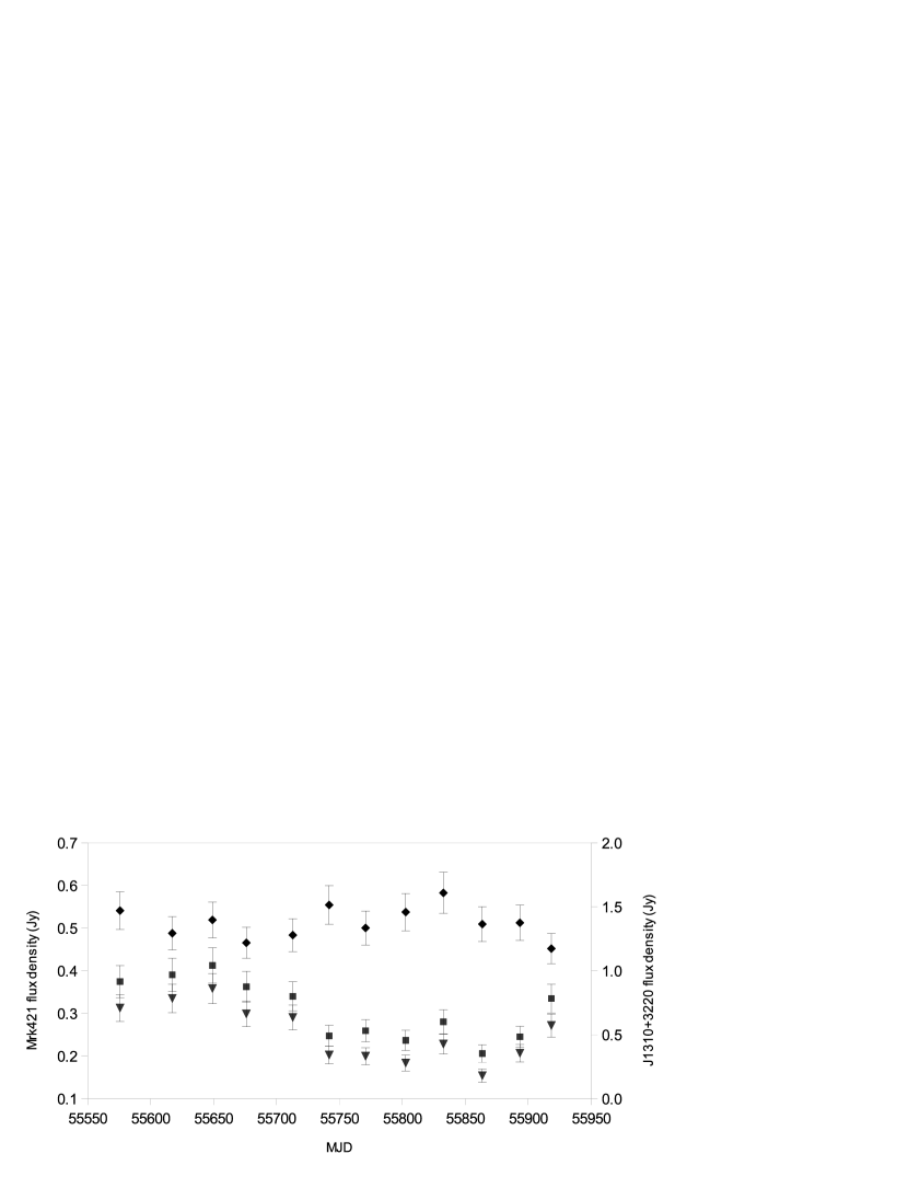
Figure 4: Light curves for Mrk421 (squares represents the total flux density and triangles represent the core flux density) and the calibrator J1310+3220 (diamonds represent the total flux density, with scale given on the right hand $y$-axis). The upper and lower panels refer respectively to the 15 GHz and 24 GHz data.

3.4 Spectral index analysis

Thanks to our multi-frequency data set, we were able to carry out a detailed analysis of the spectral index distribution on the parsec scale. We conducted a quantitative assessment of the spectral index of the components by comparing the flux density at the two frequencies at each epoch and averaging the results to reduce the statistical fluctuations. For the core, we obtained a value of $\alpha\sim-0.3\pm 0.2$, and for the outermost components (C1, C2, and C3, considered altogether), we obtained $\alpha\sim-1.2\pm 0.5$. The uncertainties were calculated from the theory of the propagation of errors using the formula

$$\Delta\alpha=\frac{1}{\log(24/15)}\sqrt{\left(\frac{\Delta S_{15}}{S_{15}}\right)^{2}+\left(\frac{\Delta S_{24}}{S_{24}}\right)^{2}},$$ (1)

where $S$ and $\Delta S$ represent the flux density and the respective uncertainty (see the last paragraph of section 3.3). These values agree with the results obtained from the spectral index image, which we produced with the following procedure: we first produced new images for each epoch and frequency using the same $(u,v)$ range and the same restoring beam ($0.4$ mas $\times$ $0.7$ mas). We then produced the spectral index image by combining the two images, resulting respectively from the stacking of all images at 15 GHz and at 24 GHz, using the AIPS task COMB, clipping the pixels with a S/N $<$ 3 using the input images. By summing images we were able to increase the S/N, and results are more reliable; the stability of the individual features guarantees that we do not lose structural information in the averaging process. The alignment of the images at the two frequencies was checked by comparing the pixel position of the peak. When a shift was present, we used the LGEOM task in AIPS to align the images. The resulting image presents the typical flat spectrum in the core region, with a steepening along the jet radius. However, despite the higher S/N obtained with image stacking, a significant spread in the spectral index values is present in the diffuse jet region, hence we do not show the image here.

3.5 Apparent speeds

From our model-fit, we infer a small or no displacement for the jet components. To verify and quantify this statement, we determined the speeds of each component by means of linear fits to the separation of the individual features from the core at different epochs. For the three outer components (C1, C2, and C3), we used combined data at 15 and 24 GHz, since the positions of each component at the two frequencies are generally consistent within the error bars. For the two inner components (C4a and C4b), we only used data at 24 GHz. Results are shown in Table 3.

We found low values for the apparent speeds, in agreement with previous studies (e.g. Piner & Edwards 2005). The two innermost components (C4a and C4b) are essentially stationary, with an upper limit to their separation velocity of $\sim 0.1$c. In addition C2 and C3 are consistent with being stationary, while the outermost component C1 has a low-significance (1.5$\sigma$) subluminal motion$\sim 0.3$c. If this trend of increasing velocity at larger radii were real and if the apparent speeds shown in Table 3 represented the bulk apparent speed of the plasma in the jet, we could speculate that some mechanism involving an acceleration acts in the outer region of the jet.

Table 3: Apparent speeds from the linear fit analysis.

Component	Apparent speed	$\beta_{\rm app}$
	(mas/yr)
C1	$0.17\pm 0.12$	$0.34\pm 0.24$
C2	$0.08\pm 0.10$	$0.16\pm 0.20$
C3	$0.05\pm 0.06$	$0.10\pm 0.11$
C4a	$-0.01\pm 0.09$	$-0.02\pm 0.17$
C4b	$-0.02\pm 0.06$	$-0.03\pm 0.11$

3.6 Jet/counter-jet ratio

We estimated the ranges of viewing angles $\theta$ and of $\beta$ from the jet/counter-jet brightness ratio. Assuming that the source has two symmetrical jets of the same intrinsic power, we used the equation

$$\frac{B_{J}}{B_{cJ}}=R=\left(\frac{1+\beta\cos\theta}{1-\beta\cos\theta}\right)^{2-\alpha},$$

where $B_{J}$ and $B_{cJ}$ are, respectively, the jet and counter-jet brightnesses and $\alpha$ represents the spectral index defined in the introduction; we adopted the $(2-\alpha)$ exponent, since the jet is smooth and does not contain well-defined compact blobs. For the jet brightness, we used $B_{J}\sim 28.4$ mJy/beam, measured at 24 GHz, in the image resulting from the stacking of all the 12 epoch images, in the jet region located at $\sim 1$ mas from the core. For the counter-jet, which is not visible, we used an upper limit provided by the $3\sigma$ rms noise level measured in the image, which resulted in $B_{cJ}=0.11$ mJy/beam; this consequently yields a lower limit to both $R$ and $\beta\cos\theta$. With a value of $\alpha=-0.4$, in agreement with our spectral index images, we obtained $R>254.8$ and then $\beta\cos\theta>0.82$. Therefore, the minimum allowed jet bulk velocity is $\beta_{\rm min}=0.82$ (corresponding to a bulk Lorentz factor $\gamma>1.74$) and the maximum viewing angle is $\theta_{\rm max}=35.0^{\circ}$.

4 Discussion and conclusions

The Doppler factor defined as

$$\delta=\frac{1}{\gamma(1-\beta\cos\theta)}$$

is a key element in the study of blazars, since it affects various parameters such as the observed brightness, the SED peak frequency, the variability timescale, and more. Modeling of the SED and study of the variability in different wavebands generally require large values of the blazar Doppler factors; in the case of Mrk421, Gaidos et al. (1996) estimated $\delta>9$, from the observed TeV variability time of about 30 min and Abdo et al. (2011) required a Doppler factor between 20 and 50 to reproduce the broadband SED. In turn, VLBI observations can also constrain $\delta$ by posing limits on $\beta$ and $\theta$, as provided by the various arguments discussed in this work.

When closely spaced repeated observations are available, the study of the proper motion is a useful tool in determining the ranges for $\beta$ and $\theta$. Surprisingly, several works (e.g. Giroletti et al. 2004b; Piner et al. 2008, 2010) have reported subluminal motions, sometimes consistent with the component being stationary, in the jets of all the $\sim$10 TeV blazars for which proper motion studies have been performed in the literature. Thanks to the large number of dual-frequency observations, the fine time-sampling, and the high quality of the data provided by the good $(u,v)$-coverage, we performed a robust identification of the Gaussian components and constrained their motion to be consistent with no displacement at all. At the same time, the high sensitivity and in particular the stacked image place significant constraints on the jet/counter-jet ratio.

The first immediate consequence is that we can reject the hypothesis that the small $\beta_{\rm app}$ is solely due to a projection effect, since it would require an unrealistically narrow viewing angle: in the case of component C4b, the upper limit to the observed motion implies a viewing angle $<1.3^{\circ}$ to reproduce the observed jet/counter-jet ratio (and even smaller to agree with the high energy limits). If the jets’ distribution is isotropic on the sky, the real number of misaligned sources (parent population) is incompatible with these very small values of $\theta$. For example, in the Bologna Complete Sample selected by Giovannini et al. (2005) at low frequency (and thus free from Doppler favoritism bias), one would expect fewer than 0.03 sources with $\theta<1.3^{\circ}$ (see also Tavecchio 2005; Henri & Saugé 2006).

On the other hand, since larger values of the viewing angle capable of reproducing the observed lack of proper motion are incompatible with the jet/counter-jet ratio, we conclude that the pattern velocity cannot be representative of the bulk flow velocity. The Gaussian components obtained in our model fit provide a good description of the visibility data but do not represent well-defined, high-contrast jet features (see Lyutikov & Lister 2010). In our interpretation, the low apparent speeds found imply that the proper motion of Mrk421 does not provide any information about the jet bulk velocity; even on the basis of the sole jet brightness ratio, untenable viewing angles would be necessary to match the pattern and bulk velocities.

What then are the real values of the viewing angle and the jet bulk velocity in Mrk421? To reproduce the observed jet asymmetry, we needed to consider a range of velocities $0.82<\beta<1$ and angles $0^{\circ}<\theta<35.0^{\circ}$. We could exclude the upper range of the $\theta$ values, since this would not reproduce the high Doppler factors required by high energy observations (Gaidos et al. 1996; Abdo et al. 2011); in particular, we were unable to achieve $\delta>20,10,5,3$ when $\theta>3.0^{\circ},5.7^{\circ},11.5^{\circ},19.4^{\circ}$, respectively.

Smaller angles thus seem to be favored since they were the only ones consistent with high values of $\delta$; however, such small angles would still represent a challenge to the observed radio properties. We were able to estimate the intrinsic power of the radio core $P_{c}^{\rm intr}$, by debeaming the observed monochromatic luminosity of the core $P_{c}^{\rm obs}$ with the equation

$$P_{c}^{\rm obs}=P_{c}^{\rm intr}\times\delta_{c}^{2-\alpha}.$$

With a value of $P_{c}^{\rm obs}\sim 6.8\times 10^{23}$ W Hz^-1 at 15 GHz, $\alpha=-0.3$, and $\delta=20$, we obtained for the intrinsic power of the core $P_{c}^{\rm intr}\sim 5.8\times 10^{20}$ W Hz^-1; this value was at the very low end of the typical range of intrinsic power found for different samples of radio galaxies (e.g. Liuzzo et al. 2011), suggesting that lower values of $\delta$ provide a more typical core power.

Moreover, the 12 monthly observations have not revealed any dramatic flux-density variability in the core of the source, which further points to a lower Doppler factor for the radio jet. We estimated the variability brightness temperature of the core ($T_{\rm B,var}$) with the formula proposed by Hovatta et al. (2009)

$$T_{\rm B,var}=1.548\times 10^{-32}\frac{\Delta S_{\rm max}d_{L}^{2}}{\nu^{2}\tau^{2}(1+z)},$$

where $\nu$ is the observed frequency in GHz, $z$ is the redshift, $d_{L}$ is the luminosity distance in meters, $\Delta S_{\rm max}$ is the difference between the maximum value for the core flux density and the minimum value, and $\tau$ is the variability time. With the values provided by our observations and $\tau$ $\sim$ 90 days, we obtaind a value of $T_{\rm B,var}\sim 2.1\times 10^{10}$ K, which does not require any significant beaming.

We similarly calculated $T_{\rm B}$ for the most compact component following the standard formula (Piner et al. 1999; Tingay et al. 1998)

$$T_{\rm B}=1.22\times 10^{12}\frac{S(1+z)}{ab\nu^{2}},$$

where $S$ is the flux density of the component measured in Jy, $a$ and $b$ are the full widths at half maximum of the major and minor axes respectively of the component measured in mas, $z$ is the redshift, and $\nu$ is the observation frequency in GHz. The resulting $T_{\rm B}$’s are on the order of a few $\times 10^{11}$ K, only slightly exceeding the limit derived by Readhead (1994) from equipartition arguments.

Taken together, the lack of superluminal features, the low core dominance, and the weak variability suggest a scenario in which no strong beaming is required in the radio jet. This is not uncommon in TeV blazars (Piner & Edwards 2004; Piner et al. 2008), but unprecedentedly firm observational support for it has been provided by our intensive campaign. Low values of the Doppler factor, e.g. $\delta\sim 3$, can reproduce the observational radio properties, including the jet brightness asymmetry.

We conclude that the Doppler factor must be different in the radio band than the $\gamma$-ray band. Since we do not expect that the viewing angle changes significantly, this leads us to the necessity of a velocity structure in the jet, as previously discussed by e.g. Chiaberge et al. (2000), Georganopoulos & Kazanas (2003), and Ghisellini et al. (2005). Our images do not provide strong evidence in favour of either a radial or transverse velocity structure, although previous works have revealed a limb brightening in Mrk421, on both a milliarcsecond scale at 43 GHz (Piner et al. 2010) and at $d>10$ mas at 5 GHz (Giroletti et al. 2006). This would favor the presence of a transverse velocity structure across the jet axis. This structure consists of two components: a fast inner spine and a slower outer layer. Different Doppler factors were obtained depending on whether we measured the speed of the spine or the layer.

A viable scenario for Mrk421 is that the viewing angle is between $2^{\circ}$ and $5^{\circ}$, which is consistent with the statistical counts of low-power radio sources and the possibility of reaching the high Doppler factors required by SED modeling and high-energy variability. The jet velocity is structured, with a typical Lorentz factor of $\gamma\sim 1.8$ in the radio region (yielding $\delta\sim 3$), and $\gamma\sim\delta\sim 20$ in the high-energy emission region. For example, assuming $\theta=4^{\circ}$, $\beta_{\rm h.e.}=0.998$, and $\beta_{\rm r}=0.82$, we obtained a value of $\delta_{\rm h.e.}=14.3$ and $\delta_{\rm r}=3.2$ and successfully reproduced all the observational properties of the source.

In summary, the detailed analysis presented in this paper has largely confirmed with improved quality expectations based on the knowledge so far achieved for TeV blazars. We have also estimated with a good level of significance some important and fundamental parameters ($\delta$, $\theta$, $\beta$, $\alpha$) that characterize the physical processes in blazars. However, there is still much to be understood and we expect to obtain other significant results from the analysis extended to other wavelengths, particularly in the $\gamma$-ray domain. Additional works on the dataset presented in this paper are planned, and will deal with, e.g., the 43 GHz images and the polarization properties. Moreover, we intend to combine our dataset with those of other works (e.g. Piner & Edwards 2005 or the MOJAVE survey, Lister et al. 2009) to increase the temporal coverage of the observations and obtain even tighter constraints over a longer time frame.

Table 4: Gaussian models.

Epoch	Frequency	Component ID	S	$\sigma_{S}$	r	$\sigma_{r}$	PA	a		$\Phi$
	(GHz)		(mJy)	(mJy)	(mas)	(mas)	(deg)	(mas)	b/a	(deg)
14/01/11	15	Core	350	35	…	…	…	0.16	0.71	-20.0
		C4	30	3.1	0.52	0.08	-43.6	0.31	1.00	…
		C3	22	2.3	1.17	0.08	-41.7	0.44	1.00	…
		C2	8.6	1.0	1.93	0.08	-36.6	0.80	1.00	…
		C1	14	1.5	3.85	0.10	-34.1	1.73	1.00	…
	24	Core	312	31	…	…	…	0.11	0.32	27.3
		C4b	23	2.4	0.26	0.06	-49.3	0.26	1.00	…
		C4a	17	1.8	0.79	0.06	-39.2	0.43	1.00	…
		C3	8.1	1.0	1.3	0.06	-45.1	0.30	1.00	…
		C2	7.1	0.9	1.91	0.06	-35.3	0.80	1.00	…
		C1	5.9	0.8	3.98	0.27	-33.5	1.49	1.00	…
25/02/11	15	Core	386	39	…	…	…	0.10	0.65	43.7
		C4	19	2.2	0.42	0.09	-44.8	0.19	1.00	…
		C3	19	1.3	1.08	0.09	-39.8	0.44	1.00	…
		C2	8.4	1.3	1.91	0.09	-44.8	0.91	1.00	…
		C1	14	1.7	4.06	0.09	-32.9	1.29	1.00	…
	24	Core	335	34	…	…	…	0.07	1.00	…
		C4b	21	2.1	0.24	0.05	-16.0	0.32	1.00	…
		C4a	14	0.9	0.71	0.05	-35.6	0.36	1.00	…
		C3	6.6	0.9	1.29	0.05	-44.2	0.28	1.00	…
		C2	5.3	0.8	1.91	0.07	-34.6	0.80	1.00	…
		C1	6.7	0.9	3.89	0.17	-33.9	1.17	1.00	…
29/03/11	15	Core	379	38	…	…	…	0.04	1.00	…
		C4	16	1.7	0.46	0.08	-34.8	0.28	1.00	…
		C3	21	2.1	1.2	0.08	-36.0	0.46	1.00	…
		C2	4.7	0.7	1.86	0.08	-45.2	0.78	1.00	…
		C1	15	1.6	3.82	0.08	-34.3	1.34	1.00	…
	24	Core	358	36	…	…	…	0.06	1.00	…
		C4b	15	1.6	0.32	0.05	-28.9	0.21	1.00	…
		C4a	13	1.5	0.83	0.05	-32.7	0.25	1.00	…
		C3	10	1.2	1.2	0.05	-44.1	0.43	1.00	…
		C2	5.7	0.9	1.96	0.06	-37.3	0.72	1.00	…
		C1	8.5	1.1	4.03	0.25	-36.2	1.31	1.00	…
25/04/11	15	Core	367	37	…	…	…	0.11	0.85	-12.4
		C4	22	2.4	0.45	0.07	-33.6	0.25	1.00	…
		C3	20	2.2	1.21	0.07	-36.7	0.41	1.00	…
		C2	6.7	1.1	2.11	0.07	-46.6	0.85	1.00	…
		C1	16	1.8	3.95	0.12	-33.1	1.47	1.00	…
	24	Core	299	30	…	…	…	0.05	1.00	…
		C4b	27	2.9	0.2	0.05	-41.7	0.12	1.00	…
		C4a	9.4	1.4	0.81	0.05	-32.6	0.26	1.00	…
		C3	10	1.4	1.35	0.05	-39.0	0.37	1.00	…
		C2	5.2	1.1	2.14	0.35	-38.6	1.04	1.00	…
		C1	11	1.5	4.32	0.28	-33.6	1.23	1.00	…
31/05/11	15	Core	346	35	…	…	…	0.04	1.00	…
		C4	24	2.5	0.4	0.07	-29.4	0.25	1.00	…
		C3	17	1.8	1.26	0.07	-33.6	0.40	1.00	…
		C2	4.7	0.9	1.81	0.07	-43.0	0.53	1.00	…
		C1	15	1.7	4.09	0.18	-34.4	1.72	1.00	…
	24	Core	290	29	…	…	…	0.04	1.00	…
		C4b	18	2.0	0.31	0.05	-18.0	0.18	1.00	…
		C4a	10	1.3	0.74	0.05	-31.0	0.29	1.00	…
		C3	7.5	1.1	1.23	0.05	-42.1	0.41	1.00	…
		C2	4.5	1.0	2.01	0.05	-34.2	0.53	1.00	…
		C1	8.9	1.2	4.45	0.35	-35.8	1.35	1.00	…
29/06/11	15	Core	263	26	…	…	…	0.19	0.41	-16.8
		C4	26	2.7	0.47	0.07	-30.8	0.26	1.00	…
		C3	16	1.7	1.2	0.07	-37.0	0.51	1.00	…
		C2	6.1	0.8	1.86	0.07	-35.9	0.61	1.00	…
		C1	19	1.9	4.08	0.16	-36.8	2.01	1.00	…
	24	Core	202	20	…	…	…	0.08	1.00	…
		C4b	27	2.9	0.23	0.04	-26.3	0.20	1.00	…
		C4a	12	1.6	0.59	0.04	-28.5	0.23	1.00	…
		C3	13	1.7	1.19	0.04	-37.0	0.51	1.00	…
		C2	6.3	1.3	2.13	0.14	-39.7	0.75	1.00	…
		C1	15	1.9	4.12	0.80	-32.9	2.56	1.00	…
28/07/11	15	Core	231	23	…	…	…	0.23	0.30	-19.4
		C4	26	2.6	0.5	0.07	-30.6	0.30	1.00	…
		C3	14	1.6	1.29	0.07	-35.6	0.45	1.00	…
		C2	5.5	0.8	2.45	0.07	-38.3	0.99	1.00	…
		C1	9.3	1.1	4.45	0.24	-35.5	1.82	1.00	…
	24	Core	199	20	…	…	…	0.14	0.56	-30.9
		C4b	28	2.9	0.29	0.05	-25.3	0.25	1.00	…
		C4a	10	1.4	0.77	0.05	-34.4	0.41	1.00	…
		C3	10	1.3	1.36	0.05	-35.4	0.55	1.00	…
		C2	2.2	0.9	2.13	0.21	-35.4	0.70	1.00	…
		C1	7.9	1.2	3.95	0.80	-35.5	2.36	1.00	…
29/08/11	15	Core	267	27	…	…	…	0.15	0.64	-21.5
		C4	30	3.1	0.33	0.07	-33.3	0.38	1.00	…
		C3	16	1.7	1.2	0.07	-32.0	0.42	1.00	…
		C2	4.6	0.7	1.97	0.07	-43.9	0.64	1.00	…
		C1	13	1.4	3.98	0.17	-34.8	1.86	1.00	…
	24	Core	183	18	…	…	…	0.03	1.00	…
		C4b	30	3.1	0.22	0.05	-18.0	0.17	1.00	…
		C4a	10	1.3	0.78	0.05	-28.9	0.37	1.00	…
		C3	4.5	0.9	1.39	0.05	-40.9	0.28	1.00	…
		C2	3.6	0.9	2	0.09	-31.5	0.66	1.00	…
		C1	6.5	1.0	4.19	0.80	-41.0	2.02	1.00	…
28/09/11	15	Core	251	25	…	…	…	0.15	0.58	12.2
		C4	34	3.5	0.33	0.08	-34.3	0.39	1.00	…
		C3	18	1.9	1.15	0.08	-32.1	0.59	1.00	…
		C2	4.2	0.9	2.02	0.13	-43.6	1.13	1.00	…
		C1	12	1.5	4.3	0.34	-32.9	2.26	1.00	…
	24	Core	228	23	…	…	…	0.09	0.42	15.2
		C4b	24	2.5	0.27	0.06	-31.0	0.15	1.00	…
		C4a	15	1.7	0.8	0.06	-30.9	0.42	1.00	…
		C3	3.3	0.8	1.35	0.06	-44.4	0.55	1.00	…
		C2	2.7	0.8	1.85	0.06	-29.0	0.43	1.00	…
		C1	9.2	1.2	4.19	0.80	-33.0	2.19	1.00	…
29/10/11	15	Core	255	25	…	…	…	0.15	0.32	-33.2
		C4	24	2.6	0.47	0.09	-34.3	0.28	1.00	…
		C3	17	1.8	1.12	0.09	-31.7	0.44	1.00	…
		C2	3.0	0.8	1.71	0.09	-35.4	0.44	1.00	…
		C1	11	1.4	4.18	0.24	-33.0	1.98	1.00	…
	24	Core	154	15	…	…	…	0.04	1.00	…
		C4b	21	2.1	0.23	0.06	-23.2	0.18	1.00	…
		C4a	11	1.2	0.8	0.06	-31.5	0.35	1.00	…
		C3	3.3	0.5	1.29	0.06	-32.8	0.41	1.00	…
		C2	3.2	0.5	1.97	0.08	-35.9	0.83	1.00	…
		C1	8.6	1.0	4.23	0.41	-33.0	1.99	1.00	…
28/11/11	15	Core	285	28	…	…	…	0.18	0.15	-14.1
		C4	19	2.1	0.48	0.08	-33.4	0.36	1.00	…
		C3	14	1.7	1.29	0.08	-32.3	0.41	1.00	…
		C2	4.8	1.0	2.04	0.08	-35.5	0.87	1.00	…
		C1	4.8	1.0	3.86	0.16	-33.3	1.17	1.00	…
	24	Core	207	21	…	…	…	0.14	0.58	-22.7
		C4b	17	1.7	0.34	0.05	-24.4	0.34	1.00	…
		C4a	6.7	0.8	0.87	0.05	-33.7	0.36	1.00	…
		C3	7.3	0.9	1.35	0.05	-33.7	0.46	1.00	…
		C2	2.7	0.6	2.1	0.05	-32.2	0.68	1.00	…
		C1	6.0	0.8	3.92	0.28	-32.4	1.44	1.00	…
23/12/11	15	Core	230	23	…	…	…	0.07	1.00	…
		C4	14	1.5	0.39	0.07	-27.0	0.38	1.00	…
		C3	12	1.3	1.17	0.07	-32.7	0.50	1.00	…
		C2	5.8	0.7	2.05	0.07	-35.0	0.74	1.00	…
		C1	6.2	0.8	4.16	0.21	-31.4	1.53	1.00	…
	24	Core	271	27	…	…	…	0.04	1.00	…
		C4b	30	3.1	0.16	0.05	-19.5	0.16	1.00	…
		C4a	16	1.8	0.61	0.05	-28.5	0.29	1.00	…
		C3	12	1.3	1.23	0.05	-39.4	0.55	1.00	…
		C2	6.2	0.9	2.04	0.05	-35.0	0.74	1.00	…
		C1	2.6	0.7	4.15	0.80	-31.4	1.53	1.00	…

Table 4: Continued.