Free fermions on a line: asymptotics of the entanglement entropy and entanglement spectrum from full counting statistics

Abstract

We consider the entanglement entropy for a line segment in the system of noninteracting one-dimensional fermions at zero temperature. In the limit of a large segment length $L$, the leading asymptotic behavior of this entropy is known to be logarithmic in $L$. We study finite-size corrections to this asymptotic behavior. Based on an earlier conjecture of the asymptotic expansion for full counting statistics in the same system, we derive a full asymptotic expansion for the von Neumann entropy and obtain first several corrections for the Rényi entropies. Our corrections for the Rényi entropies reproduce earlier results. We also discuss the entanglement spectrum in this problem in terms of single-particle occupation numbers.

1. Introduction.—

Entanglement is one of the central concepts of modern quantum mechanics and quantum information theory. It characterizes the amount of correlations between parts of a quantum system. In recent years, a progress has been achieved in studying entanglement for a variety of models, with the most detailed results available for one-dimensional systems, see e.g. the review latorre:09 .

Entanglement can be introduced in a particularly simple way in the case of a many-body system in a pure state, e.g., in the zero-temperature ground state, which will always be assumed in this paper. Let such a system be divided into two subsystems $A$ and $B$. Then the entanglement may be characterized by the properties of the reduced density matrix $\rho_{A}$ of the subsystem $A$, which is obtained by tracing out the remaining degrees of freedom

$$\rho_{A}=\operatorname{tr}_{B}\rho$$ (1)

(here $\rho$ denotes the density matrix of the pure state of the total system). The (von Neumann) entanglement entropy is then defined as the von Neumann entropy of $\rho_{A}$,

$$\mathcal{S}^{(A)}=-\operatorname{tr}\rho_{A}\ln\rho_{A}\,.$$ (2)

Though characterizing entanglement by a single number is appealing, it falls short in representing its full complexity. A more complete description of entanglement may be given by the set of Rényi entropies

$$\mathcal{S}^{(A)}_{\alpha}=\frac{1}{1-\alpha}\ln\operatorname{tr}\rho_{A}^{\;\alpha}\,,\quad\alpha\geq 0\,,\quad\alpha\neq 1$$ (3)

(the von Neumann entropy can then be expressed as the limit $\mathcal{S}^{(A)}=\lim_{\alpha\to 1}\mathcal{S}^{(A)}_{\alpha}$).

Since the total system is assumed to be in a pure state, these definitions can be shown to be symmetric with respect to the interchange of the subsystems $A$ and $B$: $\mathcal{S}^{(A)}=\mathcal{S}^{(B)}$ for both von Neumann and Rényi entropies latorre:09 , so we shall drop the superscript $(A)$ or $(B)$ in our notation below.

Equivalently, entanglement may be characterized by the spectrum of the reduced density matrix $\rho_{A}$ (which coincides with the spectrum of $\rho_{B}$ for a pure state) li:08:calabrese:08:fidkowski:10:pollmann:10 . Like the full knowledge of the Rényi entropies, the entanglement spectrum allows to determine the state of the system up to unitary transformations in the subsystems $A$ and $B$. In this sense, the Rényi entropies and the entanglement spectrum contain the full information about entanglement.

The problem of calculating the entropies or the entanglement spectrum simplifies in the case of noninteracting particles (bosons or fermions). In this case, the reduced density matrix ($\rho_{A}$ or $\rho_{B}$) can be factorized into density matrices of individual single-particle levelsd-matrix , and both the entanglement spectrum and the entropies may be expressed in terms of single-particle occupation numbers $p_{i}$. In the case of noninteracting fermions, the entropies are given by

$$\mathcal{S}=-\sum_{i}\left[p_{i}\ln p_{i}+(1-p_{i})\ln(1-p_{i})\right]$$ (4)

for the von Neumann entropy and

$$\mathcal{S}_{\alpha}=\frac{1}{1-\alpha}\sum_{i}\ln\left[p_{i}^{\alpha}+(1-p_{i})^{\alpha}\right]$$ (5)

for the Rényi entropies. The sums over $i$ can be converted into integrals over $p_{i}$ [Eqs. (26) and (27) below] by introducing the spectral density of the occupation number

$$\mu(p)=\sum_{i}\delta(p-p_{i})\,.$$ (6)

This spectral density, together with the entanglement entropies (4) and (5), in the model of noninteracting one-dimensional fermions, will be the main object of our study.

Note that, in the case of noninteracting particles, the same spectrum of occupation numbers $p_{i}$ defines the full counting statistics (FCS) of the number of particles in each of the two subsystems. This observation was used in Refs. song:11:12:klich:09:calabrese:12 to establish an exact relation between the FCS and the entanglement spectrum. In the case of noninteracting fermions, both the FCS and the entanglement spectrum can be expressed in terms of the spectrum of a single-particle correlation matrix (in the context of FCS, such a decomposition was done in Ref. abanov:08:09 on the basis of the Levitov-Lesovik determinant formula levitov:93:96 ).

Moreover, for noninteracting fermionic systems with translational invariance, the corresponding spectral problem involves matrices of Toeplitz type. Therefore, the asymptotic behavior of FCS and entanglement spectrum in the limit of a large subsystem size may be obtained with the help of the theory of Toeplitz determinants. A prominent example is the spin-1/2 $XX$ chain jin:04 ; its:09 , which can be mapped to a system of noninteracting fermions via a Jordan-Wigner transformation. In many interesting one-dimensional situations (including free fermions), the relevant Toeplitz matrix has Fisher-Hartwig singularities, and the asymptotic behavior of its determinant can be found using the Fisher-Hartwig conjecture basor:91:deift:11 . While the leading asymptotic behavior of entanglement and FCS can be obtained by choosing the main Fisher-Hartwig branch, finding subleading contributions requires more work. Recently, corrections to the entanglement entropies accurate to order $\mathcal{O}(L^{-3})$ (for a block of size $L$) have been computed for the spin-1/2 $XX$ chain calabrese:10 and in the continuous limit calabrese:11 .

Furthermore, in the continuous limit, a full asymptotic expansion of the corresponding Toeplitz determinant was conjectured in Ref. ivanov:11 in the context of FCS. Based on the matrix Riemann-Hilbert problem cheianov:04 and, independently, on the Painlevé V equation in the Jimbo-Miwa form jimbo:80:tracy:93 , an expansion was constructed for the FCS generating function of the particle number on a line interval for one-dimensional free fermions in the zero-temperature ground state. Using the periodicity conjecture for the expansion (not proven, but verified up to high orders in $1/L$), the asymptotic expansion was written in an explicitly periodic Fisher-Hartwig form ivanov:11 . Instead of selecting the leading Fisher-Hartwig branch, all the branches were combined to obtain a full expansion to all orders in $1/L$, taking into account the switching of branches intrinsically.

We use the relation between FCS and entanglement entropies to carry over the full expansion conjectured in Ref. ivanov:11 of the FCS generating function to the problem of finding the entanglement entropies and the entanglement spectrum for free fermions on a line. In particular, we find the power-law asymptotic expansion for the von Neumann entropy $\mathcal{S}$, compute first several coefficients, and present an algorithm for calculating the coefficients to an arbitrary order. A similar approach to the Rényi entropies $\mathcal{S}_{\alpha}$ produces an expansion with oscillating terms. For the Rényi entropies, we only compute the lowest-order terms, which agree with the previously available results calabrese:10 ; calabrese:11 . We also find finite-size corrections to the spectral density of single-particle occupation numbers $\mu(p)$.

The physical motivation for studying finite-size corrections to the entanglement entropies is twofold. First, in critical one-dimensional systems, the form of those corrections is related to the scaling dimensions of operators in the corresponding conformal field theory (CFT) cardy:10 . Second, knowing the structure of finite-size corrections is helpful for extracting the central charge of the CFT from numerical computations of the entropies finite-size-numerics .

The remaining parts of the paper are structured as follows. The next section embodies our main results. Then we review the asymptotic expansion of the FCS for one-dimensional free fermions. Subsequently we present the calculations of the spectral density $\mu(p)$ and of the von Neumann and Rényi entropies. Finally we conclude by a discussion of our results. The appendix includes details of the analysis of oscillating terms in the asymptotic expansions of the entanglement entropies.

Figure 1: The function $\tau(p)$ in Eq. (9). At the end points of the interval $[0,1]$, $\tau(p)$ tends to infinity (logarithmically).

2. Results.—

Based on the conjecture for the FCS in Ref. ivanov:11 , we derive the asymptotic power series for the entanglement entropy of free fermions on a line in the ground state:

$$\mathcal{S}(x)=\frac{1}{3}\ln(2x)+\Upsilon+\sum_{n=1}^{\infty}s_{2n}x^{-2n}\,.$$ (7)

Here $x=k_{F}L$ ($L$ is the length of the line segment for which the entanglement is computed and $k_{F}$ is the Fermi wavevector) and the constant $\Upsilon$ is given by Eq. (31). Note that this series contains only even powers of $1/x$. All the coefficients $s_{2n}$ are rational numbers which can be computed to any given order in $n$ using the methods of Ref. ivanov:11 . The first several coefficients are:

$$s_{2}=-\frac{1}{12}\,,\quad s_{4}=-\frac{31}{96}\,,\quad s_{6}=-\frac{7057}{1440}\,.$$ (8)

The leading term $(1/3)\ln(2x)$, the constant term $\Upsilon$, and the coefficient $s_{2}$ are known from earlier works jin:04 ; calabrese:10 ; calabrese:11 . In contrast to the Rényi entropies, there are no oscillating contributions to the von Neumann entropy at any order in $1/x$.

The calculation involves an expansion for the spectral density $\mu(p)$ based on the conjecture in Ref. ivanov:11 . Away from the end points $p=0$ and $p=1$ (a precise condition is formulated below), the spectral density has a quasiclassical structure with locally nearly equidistant levels. The smooth (nonoscillating) part of the spectral density is given by

$$\bar{\mu}(p,x)=\frac{1}{\pi^{2}\,p(1-p)}\left[\ln(2x)-\tau(p)\right]+\mathcal{O}(x^{-1})\,,$$ (9)

where

$$\tau(p)=\varphi^{\prime}\left[\frac{1}{2\pi}\ln\left(\frac{1-p}{p}\right)\right]\,,$$ (10)

$$\varphi(\xi)=\arg\left[\Gamma\left(\frac{1}{2}+i\xi\right)\right]\,,$$ (11)

and prime denotes the derivative of $\varphi(\xi)$ with respect to its argument. The function $\tau(p)$ is plotted in Fig. 1.

3. FCS of free one-dimensional fermions.—

We consider free spinless fermions on a continuous line. The temperature is assumed to be zero, i.e. the system is in the ground state characterized by the Fermi wavevector $k_{F}$. We will study the entanglement between two subsystems: an interval of length $L$ and the remainder of the line. Both FCS and the entanglement in this setup depend only on the dimensionless parameter $x=k_{F}L$. For example, the average number of particles on the line segment is given by $\left<N\right>=x/\pi$. The FCS generating function for the probability distribution of the particle number $N$,

$$\chi(\kappa,x)=\left<e^{i\,(2\pi\kappa)\,N}\right>,$$ (12)

was conjectured in Ref. ivanov:11 to be given by

$$\chi(\kappa,x)=\sum_{j=-\infty}^{\infty}\chi_{*}(\kappa+j,x)\,,$$ (13)

$$\chi_{*}(\kappa,x)=\exp\biggl{[}2i\kappa x-2\kappa^{2}\ln x+C(\kappa)\\ +\sum_{n=1}^{\infty}f_{n}(\kappa)\,(ix)^{-n}\biggr{]}\,,$$ (14)

$$C(\kappa)=\ln\left[G(1+\kappa)^{2}G(1-\kappa)^{2}\right]-2\kappa^{2}\ln 2\,,$$ (15)

where $G(z)$ denotes the Barnes G-function and $f_{n}(\kappa)$ are polynomials in $\kappa$, computable order by order. For our purpose, we will use the logarithm of this expansion, which for $-1/2<\kappa<1/2$ takes the form

$$\ln\chi(\kappa,x)=2i\kappa x-2\kappa^{2}\ln x+C(\kappa)\\ +\sum_{n=1}^{\infty}\;\sum_{m=-\left\lfloor\frac{n}{2}\right\rfloor}^{\left\lfloor\frac{n}{2}\right\rfloor}C_{n,m}(\kappa)\,x^{-n-4m\kappa}e^{2imx}\,,$$ (16)

where $\left\lfloor\cdot\right\rfloor$ denotes the integer part of the argument.

The coefficients $C_{n,m}(\kappa)$ can be expressed in terms of the polynomials $f_{n}(\kappa)$ order by order. They are also linearly related to the coefficients $R_{n,m}(\kappa)$ used in Ref. ivanov:11 for the expansion of the derivative (in $x$) of Eq. (16). In particular, $C_{n,0}(\kappa)=-(1/n)\,R_{n+1,0}(\kappa)$.

4. Entanglement spectrum.—

The spectral density $\mu(p)$ can be obtained from the jump of $\ln\chi(\kappa,x)$ across the line $\kappa=\pm 1/2$ (see, e.g., Ref. abanov:11 ):

$$\mu(p)=-\frac{1}{4\pi^{2}\,p(1-p)}\frac{\partial}{\partial\kappa}\ln\chi(\kappa,x)\biggr{|}_{\kappa=-(\frac{1}{2}-\varepsilon)-i\xi}^{\kappa=+(\frac{1}{2}-\varepsilon)-i\xi}\,,$$ (17)

where $\varepsilon$ is an infinitesimally small positive parameter and we introduced the parameterization

$$\xi=\frac{1}{2\pi}\ln\left(\frac{1-p}{p}\right)\,.$$ (18)

Inserting Eq. (16) into Eq. (17) and using the symmetry of the generating function $\chi(-\kappa,x)=\chi^{*}(\kappa,x)$, we arrive at

$$\mu(p)=-\frac{1}{2\pi^{2}\,p(1-p)}\operatorname{Re}\frac{\partial}{\partial\kappa}\Biggl{[}2i\kappa x-2\kappa^{2}\ln x+C(\kappa)\\ +\sum_{n=1}^{\infty}\;\sum_{m=-\left\lfloor\frac{n}{2}\right\rfloor}^{\left\lfloor\frac{n}{2}\right\rfloor}C_{n,m}(\kappa)\,x^{-n-4m\kappa}e^{2imx}\Biggl{]}_{\kappa=\frac{1}{2}-i\xi}\,.$$ (19)

Note that the $x$ dependence of each term in Eq. (19) is known. The coefficients at nonoscillating terms are determined by $C_{n,0}$, so that the smooth (nonoscillating) part of $\mu(p)$ can be calculated as

$$\bar{\mu}(p)=\frac{1}{\pi^{2}\,p(1-p)}\Big{(}\ln(2x)-\tau(p)\\ +\sum_{n=1}^{\infty}\operatorname{Re}C_{n,0}^{\prime}\left(\frac{1}{2}-i\xi\right)\,x^{-n}\Big{)}\,,$$ (20)

where $\tau(p)$ is given by Eqs. (10)–(11) and the prime denotes the derivative of $C_{n,0}(\kappa)$ with respect to $\kappa$. The first two terms in this expansion give the announced result (9).

Oscillating terms may, in turn, be collected by the “diagonals” $C_{2n,-n+l}(\kappa)$ and $C_{2n+1,-n+l}(\kappa)$ with $l=0,1,2,\dots$, contributing terms of the orders $x^{-2l}$ and $x^{-2l-1}$, respectively. The first two diagonals (with $l=0$) are easy to sum. By calculating the logarithm of the series (13)–(14) and using $f_{1}(\kappa)=2\kappa^{3}$ (see Ref. ivanov:11 ), we find

$$C_{2n,-n}(\kappa) =\frac{(-1)^{n+1}}{n}\,e^{n[C(\kappa-1)-C(\kappa)]}\,,$$ (21)

$$C_{2n+1,-n}(\kappa) =2i(-1)^{n+1}(3\kappa^{2}-3\kappa+1)\,e^{n[C(\kappa-1)-C(\kappa)]}\,.$$ (22)

Adding those contributions converts the continuous spectrum (20) into a sum of delta functions. For example, taking into account the diagonals (21) and (22) results in

$$\mu(p)=\sum_{n}\delta\left[\Phi(p,x)-\pi\left(n+\frac{1}{2}\right)\right]\,\frac{\partial\Phi}{\partial p}\,,$$ (23)

where

$$\Phi(p,x)=x+2\xi\ln(2x)-2\varphi(\xi)+\left(3\xi^{2}-\frac{1}{4}\right)x^{-1}+\mathcal{O}\left(x^{-2}\right)$$ (24)

and $\varphi(\xi)$ is given by Eq. (11).

Note that the spectrum (23) has a quasiclassical nature: the positions of quantum levels are determined by a quantization rule of Bohr-Sommerfeld type. The resulting spectrum is regularly spaced with the average density given by $(1/\pi)\,\partial\Phi/\partial p$. This can be explained by the fact that the diagonals (21) and (22) stem, in fact, only from the two leading Fisher-Hartwig branches in Eq. (13) at $\kappa=1/2$ (those with $j=0$ and $j=-1$). The spectrum is thus determined from the condition that these two branches cancel each other, which naturally leads to an expression of the form (23). Including higher-order Fisher-Hartwig branches produces modulations in the level spacing, but this effect appears only at higher orders in $1/x$.

Note also that this expansion breaks down close to the end points of the spectrum $p=1$ and $p=0$. In those regions $\tau(p)$ is large and therefore the density of states given by Eq. (20) becomes formally negative: in fact, the expansion (20) is not applicable in those regions of $p$. Indeed, the expansion parameter in Eq. (20) is $\xi/x$: this can be seen from the (unproven) fact observed in Ref. ivanov:11 that the polynomial $C_{n,0}$ has degree $n+2$ in $\kappa$ (and therefore in $\xi$). Thus the expansion (20) is only applicable at $|\xi|\ll x$. Remarkably, this condition also guarantees the positivity of $\bar{\mu}(p)$.

Our results (9)–(11) and the quasiclassical structure of the spectrum are consistent with the numerical studies of Refs. peschel:04:09 . In particular, the smooth part of the density of states in the middle of the spectrum is

$$\bar{\mu}(p=1/2)=\frac{4}{\pi^{2}}\left(\ln x+b\right)+\mathcal{O}(x^{-1})\,,$$

$$b=\ln 2-\varphi^{\prime}(0)\approx 2.657\,,$$ (25)

in agreement with the findings of those works.

5. Von Neumann and Rényi entropies.—

Once the spectral density $\mu(p)$ is known, the entropies can be calculated using the integral forms of Eqs. (4) and (5):

$$\mathcal{S}=-\int_{0}^{1}dp\,\mu(p)\,\left[p\ln p+(1-p)\ln(1-p)\right]$$ (26)

for the von Neumann entropy and

$$\mathcal{S_{\alpha}}=\frac{1}{1-\alpha}\int_{0}^{1}dp\,\mu(p)\,\ln\left[p^{\alpha}+(1-p)^{\alpha}\right]$$ (27)

for the Rényi entropies. Note that, even though the expansion (19) applies only at $|\xi|\ll x$, we may integrate in Eqs. (26) and (27) from $\xi=-\infty$ to $\xi=+\infty$ (corresponding to $0<p<1$): the contributions from large $\xi$ are exponentially smaller than all the terms of the resulting series and may be neglected.

For the von Neumann entanglement entropy, oscillating contributions vanish at all orders in $1/x$ [the integral (26) may be closed in the upper or lower half plane of the variable $\xi$, see Appendix]. Only nonoscillating contributions survive and may be found by replacing $\mu(p)$ in the integral (26) by its nonoscillating part (20). As a result, we find the power series

$$\mathcal{S}(x)=\frac{1}{3}\ln(2x)+\Upsilon+\sum_{n=1}^{\infty}s_{n}x^{-n}\,,$$ (28)

where the coefficients are given by

$$s_{n}=\int_{-\infty}^{\infty}d\xi\,\frac{\pi\xi}{\cosh^{2}(\pi\xi)}\,\operatorname{Im}C_{n,0}\left(\frac{1}{2}-i\xi\right)\,.$$ (29)

The functions $C_{n,0}(\kappa)$ may be found from the results reported in Ref. ivanov:11 or calculated order by order using the methods developed in that work. In particular, it follows from the results of Ref. ivanov:11 that $C_{2n+1,0}(\kappa)$ are polynomials odd in $\kappa$ with purely imaginary coefficients. Therefore, all the odd terms in the expansion (28) vanish, and we arrive at the result (7). Furthermore, since $C_{n,0}(\kappa)$ are polynomials with rational coefficients, all the coefficients $s_{2n}$ are rational numbers. The first three nonzero coefficients can be obtained from

$$C_{2,0}(\kappa) = -\frac{5}{2}\kappa^{4}\,,$$

$$C_{4,0}(\kappa) = \frac{25}{16}\kappa^{4}+\frac{63}{4}\kappa^{6}\,,$$ (30)

$$C_{6,0}(\kappa) = -\frac{35}{8}\kappa^{4}-\frac{889}{12}\kappa^{6}-\frac{3129}{16}\kappa^{8}\,,$$

which gives the result (8). Following this procedure [with $C_{2n,0}(\kappa)$ calculated using the method of Ref. ivanov:11 ], the coefficients $s_{2n}$ may be computed to any order, one by one, in a straightforward way.

The constant $\Upsilon$ is found to be

$$\Upsilon=-\frac{2}{\pi}\int_{-\infty}^{+\infty}d\xi\,\varphi^{\prime}(\xi)\left(\ln\left[2\cosh(\pi\xi)\right]-\pi\xi\tanh[\pi\xi]\right)\\ \approx 0.4950179081\,,$$ (31)

where the function $\varphi(\xi)$ is defined by Eq. (11). This expression for $\Upsilon$ can be shown to agree with that found in Ref. jin:04 .

In contrast, for the Rényi entropies, the oscillating parts do not vanish and can be classified in terms of the poles of the integrand of Eq. (27), see Appendix. The first orders [calculated using Eqs. (21) and (22)] are given by Eqs. (36) and (37). Calculating higher-order oscillating terms in the Rényi entropies would require knowing higher order diagonals $C_{2n,-n+l}(\kappa)$ and $C_{2n+1,-n+l}(\kappa)$ with $l\geq 1$. Although each of those coefficient can be separately calculated (using the methods of Ref. ivanov:11 ), deriving general formulas (valid for all $n$) is a tedious task, and we do not attempt it here.

6. Numercial illustration.—

To illustrate our main result (7)–(8) and to perform an additional check of the expansion conjectured in Ref. ivanov:11 , we have also computed the von Neumann entropies $\mathcal{S}(x)$ numerically and compared them to our analytical expansion (7)–(8). The numerical computation was performed in the lattice model (considered, e.g., in Ref. abanov:11 ) for blocks containing up to 1000 sites and then extrapolated to the continuous limit. This allowed us to calculate $\mathcal{S}(x)$ for $x\in[5,20]$ with the error bars not exceeding $10^{-9}$. In Fig. 2 we plot the remainder of the asymptotic series (7) $\Delta_{2n}=(1/3)\ln(2x)+\Upsilon+\sum_{m=1}^{n}s_{2m}x^{-2m}-\mathcal{S}(x)$ as a function of $x$. One can see that the remainders indeed decay as powers of $x$: in particular, $\Delta_{6}$ decays as $x^{-8}$, in agreement with our analytical prediction.

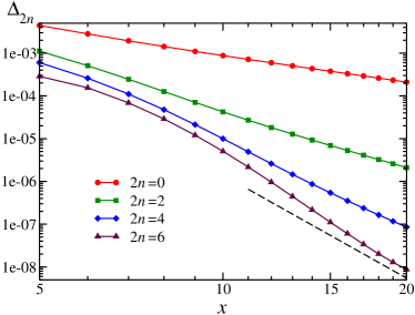
Figure 2: The remainders of the asymptotic series (7) as functions of $x$ (in the log-log scale). The dashed line indicates the slope of $x^{-8}$.

7. Summary and discussion.—

In this paper, we have used the asymptotic expansion of the FCS generating function for a line segment of one-dimensional free fermions to determine the asymptotic expansion of the entanglement entropy and the entanglement spectrum in the same system. The main result is the asymptotic power series in $1/x$ for the von Neumann entropy. Our method also allows to construct finite-size corrections for the Rényi entropies (we only do it to the lowest order, where we reproduce the known results) and gives an expansion for the spectrum of the single-particle correlation matrix.

Our results are based on the expansion conjectured (not rigorously proven) in Ref. ivanov:11 , and therefore also have the status of conjecture. Two elements of the proof were missing in Ref. ivanov:11 . First, the periodicity relations on the expansion coefficients [which allows to convert the expansion into an explicitly periodic form (13)] were not proven but only checked analytically up to the 15th order in $1/x$. Second, the expansion (13)–(14) was not extended to the line $\operatorname{Re}(\kappa)=1/2$: the point where the switching of the Fisher-Hartwig branches takes place and where we need the expansion for calculating the entropies. An extension of the expansion to this line is however a very plausible conjecture, since the expansion itself is regular at this line; it is also supported by a numerical study on the more general lattice model abanov:11 and by our numerical computations of the von Neumann entropy (Fig. 2). We thus conjecture that our results are in fact exact expressions for the model considered.

Appendix: Oscillating contributions to the entropies.—

In this appendix, we treat the oscillating (in $x$) terms in the expansions of the von Neumann and Rényi entanglement entropies. For the von Neumann entropy (26), all the oscillating terms vanish, provided the expansion conjectured in Ref. ivanov:11 is correct. For the Rényi entropies (27), there are oscillating terms decaying as $\alpha$-dependent powers of $x$.

Oscillating terms in the entropies are obtained by substituting the terms of the expansion (19) with a given oscillation frequency $m$ into the integrals (26) and (27). The integrals are further calculated by using $\xi$ as the integration variable, integrating by parts and closing the integration contour in the upper (lower) half plane for $m>0$ ($m<0$, respectively).

In the case of the von Neumann entropy, this produces terms of the form

$$\operatorname{Im}\Big{[}e^{2imx}x^{-n-2m}\int_{-\infty}^{\infty}d\xi\,\frac{\pi\xi}{\cosh^{2}(\pi\xi)}\\ \times C_{n,m}\left(\frac{1}{2}-i\xi\right)e^{4im\xi\ln x}\Big{]}\,.$$ (32)

Now the crucial ingredient of our discussion is the structure of the coefficients $C_{n,m}(\kappa)$. It can be seen from the explicit calculation in Ref. ivanov:11 (using the Riemann-Hilbert method) that these coefficients have the following form (assuming $m>0$):

$$C_{n,m}(\kappa) = \tilde{c}_{n,m}(\kappa)e^{m[C(\kappa+1)-C(\kappa)]}\,,$$ (33)

$$C_{n,-m}(\kappa) = \tilde{c}_{n,-m}(\kappa)e^{m[C(\kappa-1)-C(\kappa)]}\,,$$ (34)

where $C(\kappa)$ is defined in Eq. (15) and $\tilde{c}_{n,m}(\kappa)$ are some polynomials in $\kappa$.

From this property, it follows that, at $m>0$, the coefficient $C_{n,m}(1/2-i\xi)$ has zeroes of degree $2m$ at all points $\xi=i(1/2+r)$ for $r=0,1,\ldots$, which compensate the poles of degree two of the factor $\cosh^{-2}(\pi\xi)$ in the integral (32). Therefore the integrand is analytic in the upper half plane where the contour is closed, and the integral vanishes. Similarly, at $m<0$, the coefficient $C_{n,m}(1/2-i\xi)$ has zeroes of degree $2m$ at all points $\xi=-i(1/2+r)$ for $r=0,1,\ldots$, the integrand is analytic in the lower half plane, and the integral vanishes again. We therefore conclude that the asymptotic expansion of the von Neumann entanglement entropy has the form of a power series in $1/x$ (apart from the leading logarithm), without any oscillating terms.

In the case of the Rényi entropies, the oscillating terms have the form

$$\operatorname{Im}\Big{[}e^{2imx}x^{-n-2m}\int_{-\infty}^{\infty}d\xi\,\frac{\alpha\left[\tanh(\pi\xi)-\tanh(\alpha\pi\xi)\right]}{1-\alpha}\\ \times C_{n,m}\left(\frac{1}{2}-i\xi\right)e^{4im\xi\ln x}\Big{]}\,.$$ (35)

They contain additional poles at $\xi=\pm(i/\alpha)(1/2+n)$. These poles are not compensated by zeroes of $C_{n,m}(1/2-i\xi)$ and produce oscillating contributions to the entropy decaying as fractional ($\alpha$-dependent) powers of $x$. A calculation of the first few terms [based on the explicit expressions (21) and (22)] produces the result

$$\mathcal{S}_{\alpha}(x)=\frac{1}{6}\left[1+\frac{1}{\alpha}\right]\ln(2x)+\Upsilon_{\alpha}+\frac{(\alpha+1)(3\alpha^{2}-7)}{96\alpha^{3}}x^{-2}\\ +\sum_{n,j=1}^{\infty}\frac{(-1)^{n}}{\alpha-1}\,(2x)^{-\frac{2n(2j-1)}{\alpha}}\left[\frac{\Gamma\left(\frac{1}{2}+\frac{2j-1}{2\alpha}\right)}{\Gamma\left(\frac{1}{2}-\frac{2j-1}{2\alpha}\right)}\right]^{2n}\\ \times\left[\frac{2}{n}\cos(2nx)+x^{-1}\left[1+3\frac{(2j-1)^{2}}{\alpha^{2}}\right]\sin(2nx)\right]\\ +o(x^{-2})\,,$$ (36)

where

$$\Upsilon_{\alpha}=-\frac{2}{\pi}\int_{-\infty}^{+\infty}d\xi\,\varphi^{\prime}(\xi)\\ \times\frac{\ln\left[2\cosh(\pi\xi\alpha)\right]-\alpha\ln[2\cosh(\pi\xi)]}{1-\alpha}\,.$$ (37)

These corrections reproduce the results of Ref. calabrese:10 (in the corresponding continuous limit of the spin-1/2 $XX$ chain), calabrese:11 , and jin:04 .

References

- (1) J. I. Latorre and A. Riera, J. Phys. A: Math. and Theor. 42, 504002 (2009).
- (2) H. Li and F. D. M. Haldane, Phys. Rev. Lett. 101, 010504 (2008); P. Calabrese and A. Lefevre, Phys. Rev. A 78, 032329 (2008); L. Fidkowski, Phys. Rev. Lett. 104, 130502 (2010); F. Pollmann and J. E. Moore, New J. Phys. 12, 025006 (2010).
- (3) M.-C. Chung and I. Peschel, Phys. Rev. B 64, 064412 (2001); S.-A. Cheong and C. L. Henley, Phys. Rev. B 69, 075111 (2004); ibid. 075112 (2004); I. Peschel, J. Phys. A: Math. Gen. 36, L205 (2003); G. Vidal, J. I. Latorre, E. Rico, and A. Kitaev, Phys. Rev. Lett. 90, 227902 (2003).
- (4) H. F. Song, C. Flindt, S. Rachel, I. Klich, and K. Le Hur. Phys. Rev. B 83, 161408 (2011); H. F. Song, S. Rachel, C. Flindt, I. Klich, N. Laflorencie, and K. Le Hur, Phys. Rev. B 85, 035409 (2012); I. Klich and L. Levitov, Phys. Rev. Lett. 102, 100502 (2009); I. Klich and L. Levitov, Quantum 1134, 36 (2009); P. Calabrese, M. Mintchev, and E. Vicari, Europhys. Lett. 98, 20003 (2012).
- (5) A. G. Abanov and D. A. Ivanov, Phys. Rev. Lett. 100, 086602 (2008); Phys. Rev. B 79, 205315 (2009).
- (6) L. S. Levitov and G. B. Lesovik, Pis’ma v ZhETF 58, 225 (1993) [JETP Lett. 58, 230 (1993)]; L. S. Levitov, H.-W. Lee, and G. B. Lesovik, J. Math. Phys. 37, 4845 (1996).
- (7) B.-Q. Jin and V. Korepin, J. Stat. Phys. 116, 79 (2004).
- (8) A. Its and V. Korepin, J. Stat. Phys. 137, 1014 (2009).
- (9) E. L. Basor and C. A. Tracy, Physica A: Stat. Mech. Appl. 177, 167 (1991); P. Deift, A. Its, and I. Krasovsky, Ann. of Math. 174, 1243 (2011).
- (10) P. Calabrese and F. H. L. Essler, J. Stat. Mech.: Theory and Experiment, P08029 (2010).
- (11) P. Calabrese, M. Mintchev, and E. Vicari, Phys. Rev. Lett. 107, 020601 (2011); J. Stat. Mech. P09028 (2011).
- (12) D. A. Ivanov, A. G. Abanov, and V. V. Cheianov, arXiv:1112.2530 (2011).
- (13) V. V. Cheianov and M. B. Zvonarev, J. Phys. A: Math. and Gen. 37, 2261 (2004).
- (14) M. Jimbo, T. Miwa, Y. Môri, and M. Sato, Physica D: Nonlinear Phenomena 1, 80 (1980); C. Tracy and H. Widom, Geometric and Quantum Aspects of Integrable Systems, Lecture Notes in Physics, 424, 103 (1993).
- (15) J. Cardy and P. Calabrese, J. Stat. Mech.: Theory and Experiment, P04023 (2010).
- (16) V. V. França and K. Capelle, Phys. Rev. A 77, 062324 (2008); S. Nishimoto, Phys. Rev. B 84, 195108 (2011); B. Bauer et al, arXiv:1208.0343 (2012).
- (17) A. G. Abanov, D. A. Ivanov, and Y. Qian, J. Phys. A: Math. and Theor. 44 485001 (2011).
- (18) I. Peschel, J. Stat. Mech.: Theory and Experiment P06004 (2004); I. Peschel and V. Eisler, J. Phys. A: Math. and Theor. 42, 504003 (2009).