Magnon mediated electric current drag across a ferromagnetic insulator layer

Abstract

In semiconductor heterostructure, the Coulomb interaction is responsible for the electric current drag between two 2-d electron gases across an electron impenetrable insulator. For two metallic layers separated by a ferromagnetic insulator (FI) layer, the electric current drag can be mediated by a nonequilibrium magnon current of the FI. We determine the drag current by using the semiclassical Boltzmann approach with proper boundary conditions of electrons and magnons at the metal-FI interface.

The conventional Coulomb drag effectPogrebinskii77 ; Price88 ; Gramila91 occurs in two-dimensional electron gases separated by an insulator barrier. When one of the electron gas carries a current, the momentum transfer due to Coulomb interaction leads to a small current in the other electron gas. Recently, this current drag phenomenon has been discovered in a different system with entirely different physical mechanisms Kajiwara10 : when an electric current is injected into a Pt bar deposited on a magnetic insulator Yttrium-Iron-Garnet (YIG) film, it is found that a small electric voltage is induced in the other Pt bar, which is also deposited on the same YIG film but is located several millimeters away from the current carrying Pt bar. The authors Kajiwara10 attributed their finding to the combined effects of spin transfer torque (STT) Slonczewski ; Berger96 and spin pumping Tserkovnyak02 ; Heinrich11 : the spin Hall Hirsch99 current generated by the electric current in one Pt layer (Pt is a known material with a large spin Hall angle) is absorbed by the FI and for a sufficiently large STT, the magnetic moment of the FI begins precessing. The precessing FI pumps out a spin current to the other Pt layer. Finally, the resulting spin current converts to an electron current due to the inverse spin Hall effect Saitoh06 ; Valenzuela06 ; Kimura07 ; Madami11 ; Wang11 ; Xiao12 .

In this Letter, we propose a different geometry in which the magnon current flows normal to the plane of the layers throughout the structure. We show that the electron spin current in the metallic layers induces a nonequilibrium magnon current in the FI layer. By using semiclassical Boltzmann approach for electrons and magnons, we are able to self-consistently determine these currents and thereby obtain the drag current for given geometrical and material parameters. The resulting drag current is several orders of magnitude larger than that in the nonlocal geometry in Ref. Kajiwara10

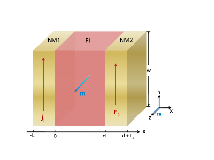
Figure 1: Schematics of the NM/FI/NM trilayer structure.

To be more specific, we consider a simple trilayer structure, shown in Fig. 1 schematically, where a ferromagnetic insulating (FI) layer is sandwiched by two heavy metal films (NM1 and NM2) such as Pt and Ta. A charge current parallel to the plane of the layers is injected in the layer NM1. To determine the drag current in the layer NM2, we first establish transport equations for each layers and then find proper boundary conditions to solve the transport coefficients.

Electron current and spin accumulation in Metallic layers. For the NM layers, a spin dependent Ohm’s law has been well established and may be written in the following form szhang00 ,

$$\mathbf{\hat{j}}=\frac{c}{2}\mathbf{\hat{E}+}\frac{c_{h}}{4}\left({\bf\hat{E}}\times\mbox{\boldmath$\sigma-\sigma$}\times\mathbf{\hat{E}}\right)$$ (1)

where the spinor current density $\hat{\bf j}$ and the electric field $\hat{\bf E}$ are $2\times 2$ vector matrices in spin space, $\sigma$ is a Paul vector matix, and $c$ and $c_{h}$ are the electric conductivity and spin Hall conductivity respectively. The second term is the spin Hall current whose anti-symmetric form is essential for $\mathbf{\hat{j}}$ to be an Hermitian in spin space (also noted that ${\bf\hat{E}}\times\mbox{\boldmath$\sigma$}\neq-\mbox{\boldmath$\sigma$}\times\mathbf{\hat{E}}$ due to non-communitivity of the Pauli matrices). The electrical field is related to the spinor chemical potential $\hat{\mu}$ via $\hat{\bf E}=-(1/e)\mbox{\boldmath${\nabla}$}\hat{\mu}$ where $e(<0)$ denotes the electron charge. While it is possible to work with an arbitrary choice of the spin quantization, we proceed below to a special case where the magnetic moment of the FI is oriented in the $z$-direction and the electric current flows in the $y$ direction. If we choose the spin quantization axis parallel to the $z$-axis, one can simply work on the two-component (spin-up and spin down) form of the Ohm’s law; i.e.,

$$j_{y}^{\alpha}(x)=\frac{c}{2}E_{y}^{\alpha}(x)-\alpha\frac{c_{h}}{2}E_{x}^{\alpha}(x)$$ (2)

and

$$j_{x}^{\alpha}(x)=\frac{c}{2}E_{x}^{\alpha}(x)+\alpha\frac{c_{h}}{2}E_{y}^{\alpha}(x)$$ (3)

where $\alpha=\pm 1$ represent spin up an down. To determine the spin dependent electric field, we recall the spin diffusion equation Valet

$$\frac{d^{2}}{dx^{2}}[\mu^{\uparrow}(x)-\mu^{\downarrow}(x)]=\frac{\mu^{\uparrow}(x)-\mu^{\downarrow}(x)}{\lambda_{sf}^{2}}$$ (4)

and its solution

$$\mu^{\uparrow}(x)-\mu^{\downarrow}(x)=A_{i}e^{-x/\lambda_{sf}}+B_{i}e^{x/\lambda_{sf}}$$ (5)

where $\lambda_{sf}$ is the electron spin diffusion length, and the constants $A_{i}$ and $B_{i}$ ($i=1$ for the NM1 layer and $i=2$ for NM2) are determined by the boundary conditions. Although these equations apply to both NM1 and NM2 layers, they have different constraints set by experimental measurement. For the NM1 layer, we take $E_{y}^{\alpha}(x)=E_{ext}$ where $E_{ext}$ is the applied electric field in the NM1 layer, while $\int_{NM2}dxj_{y}(x)=0$ in the open circuit of the NM2 layer.

Magnon current and magnon accumulation in the FI layer. For the FI layer, we start with a general magnon Boltzmann equation in the presence of spatially dependent temperature $T(x)$ and magnetic field $\mathbf{H}(x)$,

$$v_{x}\frac{\partial N_{m}}{\partial x}+v_{x}\frac{\partial N_{m}}{\partial T}\frac{dT}{dx}+v_{x}\frac{\partial N_{m}}{\partial\mathbf{H}}\cdot\frac{d\mathbf{H}}{dx}+\mathbf{\dot{q}\cdot}\frac{\partial N_{m}}{\partial\mathbf{q}}=-\left(\frac{\partial N_{m}}{\partial t}\right)_{scatt.}$$ (6)

where $N_{m}\left(x,\mathbf{q,}T(x),\mathbf{H}(x)\right)$ is the magnon distribution. The first term describes magnon diffusion. The second and third terms are responsible for the magnon transport in the presence of temperature and magnetic field gradients, which have been recently studied in the content of spincalorics Uchida10 ; Bauer10 ; Loss03 ; Xing04 . The last term on the left side of Eq. (6) is associated with acceleration of magnons by external forces such as a confining potential at boundary Matsumoto11 . The scattering term on the right side of the Eq. (6) may be modeled by the relaxation time approximation

$$\left(\frac{\partial N_{m}}{\partial t}\right)_{scatt.}=\frac{N_{m}-\bar{N}_{m}}{\tau_{m}}+\frac{N_{m}-N_{m}^{0}}{\tau_{th}}$$ (7)

where $\bar{N}_{m}(x)=\int d\mathbf{q}N_{m}(x,\mathbf{q})/\int d\mathbf{q}$ is the momentum averaged magnon distribution while $N_{m}^{0}(x,\mathbf{q})=\frac{1}{e^{\epsilon_{\mathbf{q}}/k_{B}T(x)}-1}$ is the local equilibrium magnon distribution, where $\epsilon_{\mathbf{q}}=D\mathbf{q}^{2}+\triangle_{g}$ is the magnon dispersion, $D$ is the spin wave stiffness, $\triangle_{g}$ is the spin wave gap, and $v_{x}=\frac{1}{\hbar}\frac{\partial\epsilon_{\mathbf{q}}}{\partial q_{x}}$ is the $x$ component of the magnon velocity. The first relaxation term describes those processes which conserve the number of magnons. For example, magnon scattering by a paramagnetic impurity has the form of $V_{\bf qq^{\prime}}a_{\bf q}^{+}a_{\bf q^{\prime}}$; i.e., the impurity or surface roughness Sparks64 ; Mills03 scatters the magnon ${\bf q^{\prime}}$ to the magnon ${\bf q}$. As long as we neglect the wave number dependence of the scattering matrix $V_{\bf qq^{\prime}}$, this process can be modeled by the first term of Eq. (7). The second term of Eq. (7) does not conserve the number of magnons. The magnon absorption and emission relax the nonequilibrium magnons to equilibrium ones, e.g., magnon-phonon interaction Suhl65 .

For the present system, we consider uniform temperature and magnetic field, and there is no external force on magnons. Then, Eq. (6) and (7) reduce to

$$v_{x}\frac{\partial N_{m}\left(x,\mathbf{q}\right)}{\partial x}=-\frac{N_{m}\left(x,\mathbf{q}\right)-\bar{N}_{m}\left(x\right)}{\tau_{m}}-\frac{N_{m}\left(x,\mathbf{q}\right)-N_{m}^{0}\left(\mathbf{q}\right)}{\tau_{th}}.$$ (8)

We may proceed to solve $N_{m}$ by the same way as for the electron distribution in magnetic multilayers Valet . Particularly, one may expand the nonequilibrium distribution by the Legendre polynomials,

$$N_{m}(x,\mathbf{q})=N_{m}^{0}(\mathbf{q})+\frac{\partial N_{m}^{0}(\mathbf{q})}{\partial\epsilon_{\mathbf{q}}}\left[\mu_{m}(x)+\underset{n=1}{\overset{\infty}{\sum}}g^{(n)}(x)P_{n}\left(\cos\theta\right)\right]$$ (9)

where $\mu_{m}(x)$ is the $n=0$ component of the nonequilibrium distribution and $\theta$ is the angle between $\mathbf{q}$ and $x$ axis. By placing the above equation into Eq. (8) and by utilizing the orthogonality property of the Legendre polynomials, one can arrive at a series of algebraic equations for the coefficients $g^{(n)}(x)$. In the supplemental material, we show the solutions in some limiting cases. Once the distribution functions $N_{m}({x,\bf q})$ are determined, we can find the magnon accumulation and magnon current via

$$j_{m}(x)=\frac{-2\mu_{B}}{\left(2\pi\right)^{3}}\int d\mathbf{q}v_{x}N_{m}({\bf q},x);\;\;\;\delta n_{m}(x)=\frac{1}{\left(2\pi\right)^{3}}\int d\mathbf{q}\left[N_{m}({\bf q},x)-N_{m}^{0}({\bf q})\right]$$ (10)

where $\mu_{B}$ is the Bohr magneton. Note that a magnon carries spin moment $-\gamma\hbar(=-2\mu_{B})$ where $\gamma$ is the gyromagnetic ratio.

We may further simplify the solution of the non-equilibrium magnon distribution by discarding high orders ($n\geq 2$) of the polynomials. Consequently, we find a local relation between magnon accumulation and magnon current,

$$\frac{d}{dx}j_{m}(x)=2\mu_{B}\frac{\delta n_{m}(x)}{\tau_{th}}$$ (11)

and

$$j_{m}(x)=\frac{2\mu_{B}\tau_{m}}{3}\frac{I_{2}}{I_{0}}\frac{d}{dx}\delta n_{m}(x)$$ (12)

where $I_{n}$ are integration constants $I_{n}\equiv\frac{1}{(2\pi)^{3}}\int d^{3}qv^{n}\frac{\partial N_{m}^{0}(\mathbf{q})}{\partial\epsilon_{\mathbf{q}}}$. We point out that this local current expression is valid in the limit $\tau_{th}\gg\tau_{m}$ which is a good approximation for ferromagnets Suhl65 (see supplemental material). By combining Eqs. (11) and (12), we obtain the diffusion equation for nonequilibrium magnons,

$$\frac{d^{2}}{dx^{2}}\delta n_{m}(x)-\frac{\delta n_{m}(x)}{l_{m}^{2}}=0$$ (13)

where the magnon diffusion length is defined as $l_{m}=\sqrt{\frac{I_{2}}{3I_{0}}\tau_{th}\tau_{m}}$. At room temperature ($T=300K$), for YIG with $\triangle_{g}\sim 10^{-5}eV$, $\tau_{m}\sim 10^{-7}s$ and $\tau_{th}\sim 10^{-6}s$, $l_{m}$ is estimated at $0.05cm$, consistent with the measurement Schneider08 . Equation (13) has the general solution,

$$\delta n_{m}(x)=A_{F}e^{-x/l_{m}}+B_{F}e^{x/l_{m}}$$ (14)

and thus the magnon current density reads

$$j_{m}(x)=\frac{2\mu_{B}l_{m}}{\tau_{th}}\left(-A_{F}e^{-x/l_{m}}+B_{F}e^{x/l_{m}}\right)$$ (15)

Boundary conditions. The outer-boundary conditions at $x=-L_{1}$ and $x=d+L_{2}$, where $L_{1}$, $d$ and $L_{2}$ represent the thicknesses of the layers of NM1, FI and NM2, are $j_{x}^{\uparrow,\downarrow}(-L_{1})=j_{x}^{\uparrow,\downarrow}(d+L_{2})=0$. The boundary conditions at the metal-FI interfaces depend on the interaction between electrons and magnons. Here we assume a s-d type interaction $-J_{sd}\mbox{\boldmath$\sigma$}\cdot{\bf S}_{i}$ where $\sigma$ is the itinerant electron spin of the metal layer and ${\bf S}_{i}$ is the local spin of the FI layer at the interfaces. The interaction conserves total angular momentum and thus the first boundary condition is the continuity of total spin current at the interfaces; i.e.,

$$(-\mu_{B}/e)\left[j_{x}^{\uparrow}(0^{-})-j_{x}^{\downarrow}(0^{-})\right]=j_{m}(0^{+})$$

and

$$j_{m}(d^{-})=(-\mu_{B}/e)\left[j_{x}^{\uparrow}(d^{+})-j_{x}^{\downarrow}(d^{+})\right]$$ (16)

The total angular momentum current conservation simply states that electron spin current in the metals must be converted into magnon current in the FI layer at the interfaces. If the interfaces have magnetic roughness, the spin-flip scattering by magnetic impurities can transfer spin angular momentum to lattice via spin-orbit coupling. In this case, the outgoing spin current would be reduced footnote .

The other boundary conditions at the interfaces should relate the electron spin accumulation to the non-equilibrium magnon density. Within the s-d model, one can treat the electron spin density as an effective magnetic field on the interface spin of the FI layer; i.e., $H_{eff}=J_{sd}\delta{\bf m}_{z}$ and thus

$$\mu^{\uparrow}(0^{-})-\mu^{\downarrow}(0^{-})=\varepsilon\delta n_{m}(0^{+})$$

and

$$\varepsilon\delta n_{m}(d^{-})=\mu^{\uparrow}(d^{+})-\mu^{\downarrow}(d^{+})$$ (17)

where

$$\varepsilon=\frac{4\left(\pi D\right)^{3/2}}{J_{sd}D\left(\varepsilon_{F}\right)a_{0}^{3}\cdot\sqrt{k_{B}T}Li_{\frac{1}{2}}\left(e^{-\Delta_{g}/k_{B}T}\right)}$$ (18)

$D\left(\varepsilon_{F}\right)$ is the electron density of state at Fermi level, $a_{0}$ is the lattice constant of the NM layer and $Li_{s}\left(z\right)\equiv\sum\nolimits_{k=1}^{\infty}\frac{z^{k}}{k^{s}}$ is the polylogarithm. The detailed derivation of $\varepsilon$ is arranged in the supplemental material. We note that Takahashi et al. have also proposed a boundary condition at the interface Takahashi10 which relates magnon spin current to spin accumulation; i.e., $j_{m}\propto\mu^{\uparrow}-\mu^{\downarrow}$. However, such boundary condition is unable to self-consistently determine the magnon current. On the contrary, the boundary conditions we have derived are able to uniquely determine the spin and magnon currents throughout the structure. A rough order of magnitude estimation of $\varepsilon$ can be readily obtained by using the following plausible parameters appropriate for Pt/YIG/Pt structure: $D\left(\varepsilon_{F}\right)\sim 3n_{e}/2\epsilon_{F}$, $n_{e}=5\times 10^{22}$ $cm^{-3}$, $J_{sd}=1$ $eV$, $\epsilon_{F}=5$ $eV$, $a_{0}=4$ ${\AA}$, and $D=6$ $meV\cdot nm^{2}$, and thus $\varepsilon\sim 0.2$ $meV\cdot nm^{3}$.

With the above boundary conditions, the constants in Eq. (5) and (14) can be readily determined. If one uses an Ampere meter voltmeter to measure the average (measured) induced electric current density $j_{y}^{(2)}=(1/L_{2})\int dxj_{y}^{(2)}(x)$ in NM2 layer, we find the ratio between the induced current and the injected current magnitude $\eta\left(\equiv j_{y}^{(2)}/j_{y}^{(1)}\right)$ is,

$$\eta=\left(\frac{c_{h}}{c}\right)^{2}\left(\frac{\lambda_{sf}}{L_{2}}\right)\frac{\operatorname{sech}\left(\frac{L_{2}}{\lambda_{sf}}\right)\left[\cosh\left(\frac{L_{2}}{\lambda_{sf}}\right)-1\right]}{\left[b^{-1}+b\tanh\left(\frac{L_{2}}{\lambda_{sf}}\right)\right]\sinh\left(\frac{d}{l_{m}}\right)+\left[1+\tanh\left(\frac{L_{2}}{\lambda_{sf}}\right)\right]\cosh\left(\frac{d}{l_{m}}\right)}$$ (19)

where $b=c\varepsilon\tau_{th}/(4e^{2}l_{m}\lambda_{sf})$, and $L_{1}\gg\lambda_{sf}$ is assumed for simplicity. The first prefactor $(c_{h}/c)^{2}$ origins from the two successive conversions between electric current and spin Hall current in NM1 and NM2 due to the spin Hall and inverse spin Hall effect respectively. The second prefactor $\lambda_{sf}/L_{2}$ indicates that the maximum range of the current density in NM2 is $\lambda_{sf}$; i.e., if the thickness of NM2 exceeds $\lambda_{sf}$, the average current density $j_{y}^{(2)}$ would be inversely proportional to $L_{2}$. Interestingly, when $L_{2}$ is much smaller than $\lambda_{sf}$, the induced electric current is also small; this is because the spin current at the surface $x=d+L_{2}$ is set to zero and thus the self-consistent calculation demands a small current throughout the NM2 layer. In Fig.2, we show $\eta$ as a function of the thickness of the metal layer (NM2) for Pt/YIG/Pt trilayers with several different YIG layer thicknesses. We choose the material parameters as follows: Pt layer conductivity $c_{Pt}\sim 0.1\left(\mu\Omega\cdot cm\right)^{-1}$, spin diffusion length $\lambda_{sf}=7$ $nm$ and the spin Hall angle $c_{h}/c=0.05$ Buhrman11 ; magnon diffusion length $l_{m}=0.05$ $cm$ and magnon relaxation time $\tau_{th}=10^{-6}$ $s$. We see that $\eta$ decreases as the thickness of the YIG layer increases due to the decay of magnon diffusion current. Also for fixed YIG layer thickness, $\eta$ reaches its maximum around $L_{2}=\lambda_{sf}$. The peak value of $\eta$ is of the order of $10^{-4}$. If the injected current density is $10^{6}$ $A/cm^{2}$, the induced voltage of a Pt bar with its length $w=1$ cm would be $V^{(2)}=wj_{y}^{(2)}/c\sim 1$ mV. If one replaces Pt with Ta which has larger spin Hall angle of $0.1$ Buhrman12 , $V^{(2)}$ can be further increased by a factor of 4, which is rather significant and easily detectable experimentally.

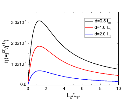
Figure 2: The ratio of the average induced current density and the injected current density as a function of the NM2(Pt) layer thickness for three different thicknesses of the FI (YIG) layer.

Finally we comment on the relation of our calculation with the experimental measurement Kajiwara10 . In their experiments, when the first Pt layer injects a spin current to the FI layer, the magnons propagate in the plane of the FI layer in order to reach the second Pt. While there is a similar non-equilibrium magnon density buildup near the second Pt layer, the direction of the magnon current and the gradient of the magnon density are in the plane of the layer. In another word, there is neither magnon current nor magnon density gradient in the direction perpendicular to the layer such that the second Pt layer is unable to receive any spin angular momentum from the FI layer. Thus, we conclude that the nonlocal setup in the experiment Kajiwara10 is not relevant to our theory. In the conventional nonlocal metallic spin valve, however, one does observe a voltage change of the entire detection bar due to the spin accumulation (not the spin current or gradient of the spin accumulation) in the channel. In the present case, we derive the induced current in the second Pt bar which is related to the spin current (or magnon density gradient) in the direction perpendicular to the layer. Furthermore, the observed current in the experimentKajiwara10 has been attributed to the STT and spin pumping, which is several orders of magnitude smaller than what we predict in our geometry.

This work is supported by NSF.

SUPPLEMENTAL MATERIALS

.1 Magnon diffusion equation in ferromagnetic insulator

In this section, we derive the magnon diffusion equation, Eq. (13), from the magnon Boltzmann equation, Eq. (8). By placing Eq. (9) into Eq. (8), we have

$$v_{x}\frac{\partial N_{m}^{0}(\mathbf{q})}{\partial\epsilon_{\mathbf{q}}}\frac{\partial g(x,\mathbf{q})}{\partial x}+\frac{\partial N_{m}^{0}(\mathbf{q})}{\partial\epsilon_{\mathbf{q}}}\left(\frac{1}{\tau_{m}}+\frac{1}{\tau_{th}}\right)g(x,\mathbf{q})$$

$$=-v_{x}\frac{\partial N_{m}^{0}(\mathbf{q})}{\partial\epsilon_{\mathbf{q}}}\frac{d\mu_{m}\left(x\right)}{dx}-\frac{\partial N_{m}^{0}(\mathbf{q})}{\partial\epsilon_{\mathbf{q}}}\frac{\mu_{m}\left(x\right)}{\tau_{th}}-\frac{\mu_{m}\left(x\right)}{\tau_{m}}\left[\frac{\partial N_{m}^{0}(\mathbf{q})}{\partial\epsilon_{\mathbf{q}}}-\bar{\frac{\partial N_{m}^{0}}{\partial\epsilon_{\mathbf{q}}}}\right]-\frac{N_{m}^{0}(\mathbf{q})-\bar{N}_{m}^{0}}{\tau_{m}}$$ (A1)

where $\bar{\frac{\partial N_{m}^{0}}{\partial\epsilon_{\mathbf{q}}}}\equiv\int d\mathbf{q}\frac{\partial N_{m}^{0}(\mathbf{q})}{\partial\epsilon_{\mathbf{q}}}/\int d\mathbf{q}$, $\bar{N}_{m}^{0}\equiv\int d\mathbf{q}N_{m}^{0}(\mathbf{q})/\int d\mathbf{q}$, and $g(x,\mathbf{q})=\underset{n=1}{\overset{\infty}{\sum}}g^{(n)}(x)P_{n}\left(\cos\theta\right)$ is the Legendre polynomial expansion of the nonequilibrium magnon distribution when a rotational symmetry is assumed.

The non-equilibrium magnon density and magnon current, as defined in Eq. (10), are simply the zeroth and first components of the Legendre polynomials,

$$\delta n_{m}(x)=4\pi I_{0}\mu_{m}(x)$$ (A2)

and

$$j_{m}(x)=-\frac{8\pi\mu_{B}}{3}I_{1}g^{(1)}(x)$$ (A3)

where we have defined

$$I_{n}\equiv\frac{1}{(2\pi)^{3}}\int d^{3}qv^{n}\frac{\partial N_{m}^{0}(\mathbf{q})}{\partial\epsilon_{\mathbf{q}}}$$ (A4)

$v=({\bf q}/q)\cdot\mbox{\boldmath$\nabla$}\epsilon_{m}({\bf q})/\hbar$ is the magnitude of magnon velocity.

The relations among $g^{(n)}$ can be readily obtained by multiplying Eq. (A1) by $v_{x}^{n}$ and integrating over ${\bf q}$,

$$\frac{d}{dx}j_{m}(x)=2\mu_{B}\frac{\delta n_{m}(x)}{\tau_{th}},\text{ \ \ \ }(n=0)$$ (A5)

$$\frac{2I_{2}}{5}\frac{d}{dx}g^{(2)}(x)+I_{1}\left(\frac{1}{\tau_{m}}+\frac{1}{\tau_{th}}\right)g^{(1)}(x)=-I_{2}\frac{d}{dx}\mu_{m}\left(x\right),\text{ \ \ \ }(n=1)$$ (A6)

and

$$I_{n+1}\left[\frac{n}{2n-1}\frac{dg^{(n-1)}}{dx}+\frac{n+1}{2n+3}\frac{dg^{(n+1)}}{dx}\right]+I_{n}\left(\frac{1}{\tau_{m}}+\frac{1}{\tau_{th}}\right)g^{(n)}=0,\text{ \ \ \ }(n\geq 2)$$ (A7)

where we have used the following orthogonal relations for the Legendre polynomials

$$\overset{1}{\underset{-1}{\int}}duP_{n^{\prime}}\left(u\right)P_{n}\left(u\right)=\frac{2}{2n+1}\delta_{n,n^{\prime}}$$ (A8)

and

$$\overset{1}{\underset{-1}{\int}}duP_{1}\left(u\right)P_{n^{\prime}}\left(u\right)P_{n}\left(u\right)=\frac{2\left(n+1\right)}{\left(2n+1\right)\left(2n+3\right)}\delta_{n^{\prime},n+1}+\frac{2n}{\left(2n+1\right)\left(2n-1\right)}\delta_{n^{\prime},n-1}$$ (A9)

At this point, the problem of solving the magnon distribution is equivalent to determining the infinite function series $g^{(n)}(x)$. To simplify the problem, we assume $\tau_{th}\gg\tau_{m}$, which is generally valid for most insulating ferromagnetic materials Suhl65 . In this case, the ratio of $g^{(n+1)}/g^{(n)}$ is about $\sqrt{\tau_{m}/\tau_{th}}$. To see it, we first neglect $g^{(2)}$ in Eq. (A6) and substitute the resulting expression for $g^{(1)}$ into Eq. (A5). One immediately sees that the spatial derivatives of both $\mu_{m}$ and $j_{m}$ scale as $1/\sqrt{\tau_{m}\tau_{th}}$. Putting this scaling back to Eq. (A6) and (A7), we confirm that neglecting $g^{(n)}$ ($n\geq 2$) is justified as long as $\tau_{th}\gg\tau_{m}$. Combining Eqs. (A2), (A3), (A5) and (A6), we arrive at the magnon diffusion equation in the main text, Eq. (13).

We emphasize that the validity of the magnon diffusion equation rests on the condition that the magnon conserving scattering is much stronger than the magnon non-conserving scattering, i.e., $\tau_{th}\gg\tau_{m}$; this condition is similar to the spin diffusion equation for electrons where the momentum scattering (spin-conserving) is stronger than the spin-flip scattering Valet93 . Thus, the magnon diffusion equation can be used for the length scale larger than the spin-conserving scattering length (e.g., it is the mean free path in the electron case) which is considered much smaller than the magnon (spin) diffusion length.

.2
Boundary conditions at metal-FI interfaces

In this section, we derive the boundary conditions Eqs. (16) and (17) by using the $s-d$ exchange coupling

$$\hat{H}=-J_{sd}\underset{i}{\mathbf{\sum}}\int d^{3}r\mathbf{s}\left(\mathbf{r}\right)\cdot\mathbf{S}\left(\mathbf{R}_{i}\right)\delta\left(\mathbf{r-R}_{i}\right),$$ (B1)

where ${\bf S}(\textbf{R}_{i})$ are the localized spins of FI at the interface in contact with the conduction electron spins $\textbf{s}(\textbf{r})$ of the metal. The above s-d interaction contains a spin-flip scattering processes of $J_{sd}(c_{{\bf k}\downarrow}^{+}c_{{\bf k-q}\uparrow}a_{\bf q}+h.c.)$ and a non-spin-flip process $J_{sd}c_{{\bf k+q^{\prime}}\sigma}^{+}c_{{\bf k+q}\sigma}a_{\bf q}^{+}a_{\bf q^{\prime}}$White68 . For the spin-flip process, the electron spin loss (gain) leads to the magnon generation (annihilation), but the total angular momentum is conserved; this leads to the first interface boundary condition of Eq. (16). For the non-spin-flip processes, we use the simple mean field approach, i.e., the conduction electron spin density is treated as an effective magnetic field acting on the interficial spins of the FI layer; i.e.,

$$\delta H_{eff}=-\frac{J_{sd}D\left(\varepsilon_{F}\right)v_{0}}{g\mu_{B}}\left(\mu^{\uparrow}-\mu^{\downarrow}\right)$$ (B2)

where $D(\varepsilon_{F})$ is the electronic density of states and $v_{0}$ is the volume of primitive cell of the metal layer. The consequence of this effective field is to induce, in linear response, a deviation in longitudinal magnetization

$$\delta M_{z}=\chi_{zz}\delta H_{eff}$$ (B3)

where $\chi_{zz}$ is the longitudinal susceptibility for interface spins of the FI layer and $\delta M_{z}$ is related to the magnon density $\delta M_{z}(x)=-2\mu_{B}\delta n_{m}(x)$. Thus, the relation between spin accumulation of non-equilibrium electron density and nonequilibrium magnon density at the metal-FI interface is

$$\mu^{\uparrow}-\mu^{\downarrow}=\varepsilon\delta n_{m}$$ (B4)

where

$$\varepsilon=\frac{g\mu_{B}^{2}}{J_{sd}D\left(\varepsilon_{F}\right)\chi_{zz}v_{0}}.$$ (B5)

$\chi_{zz}$ can be derived in linear response by $\chi_{zz}=\left.\frac{\partial M_{z}}{\partial H}\right|_{H\rightarrow 0}$ with $M_{z}=M_{S}-\frac{2\mu_{B}}{\left(2\pi\right)^{3}}\int d\mathbf{q}N_{m}^{0}\left(\mathbf{q}\right)$. In the limit $Dq_{\max}^{2}\gg k_{B}T$, we find

$$\chi_{zz}=\frac{g\mu_{B}^{2}\sqrt{k_{B}T}}{4\left(\pi D\right)^{3/2}}Li_{\frac{1}{2}}\left(e^{-\Delta_{g}/k_{B}T}\right)$$ (B6)

where $Li_{s}\left(z\right)\equiv\sum\nolimits_{k=1}^{\infty}\frac{z^{k}}{k^{s}}$ is the polylogarithm. Inserting Eq.(B6) into (B5), we get the final result $\varepsilon$ of Eq. (18).

References

- (1) M. B. Pogrebinskii, Fiz. Tekh. Poluprovodn. 11, 637 (1977) [Sov. Phys. Semicond. 11, 372 (1977)].
- (2) P. J. Price, Physica (Amsterdam) 117B, 750 (1983); in The Physics of Submicron Semiconductor Devices, edited by H. Grubin, D. K. Ferry, and C. Jacoboni (Plenum, New York, 1988).
- (3) T.J. Gramila, J.P. Eisenstein, A.H. MacDonald, L.N. Pfeiffer, and K.W. West, Phys. Rev. Lett. 66, 1216 (1991).
- (4) Y. Kajiwara et al., Nature 464, 262 (2010).
- (5) J. C. Slonczewski, J. Magn. Magn. Mater. 159, L1 (1996).
- (6) L. Berger, Phys. Rev. B 54, 9353 (1996).
- (7) Y. Tserkovnyak, A. Brataas, and G. E. W. Bauer, Phys. Rev. Lett. 88, 117601 (2002).
- (8) B. Heinrich et al.,Phys. Rev. Lett. 107, 066604 (2011).
- (9) J. E.Hirsch, Phys. Rev. Lett. 83, 1834–1837 (1999)
- (10) E. Saitoh et al., Appl. Phys. Lett. 88, 182509 (2006).
- (11) S. Valenzuela and M. Tinkham, Nature 442, 176 (2006).
- (12) T. Kimura et al., Phys. Rev. Lett. 98, 156601 (2007).
- (13) M. Madami et al., Nature Nanotechnology 6, 635 (2011).
- (14) Z. Wang, Y. Sun, M. Wu, V. Tiberkevich, and A. Slavin, Phys. Rev. Lett. 107, 146602 (2011).
- (15) J. Xiao and G.E.W Bauer, Phys. Rev. Lett. 108, 217204 (2012).
- (16) S. Zhang, Phys. Rev. Lett. 85, 393(2000).
- (17) T. Valet and A. Fert, Phys. Rev. B 48, 7099 (1993).
- (18) K. Uchida et al., Nature Mater. 9, 894 (2010).
- (19) G.E.W. Bauer, A.H. MacDonald, and S. Maekawa, Solid State Commun. 150, 459 (2010).
- (20) F. Meier and D. Loss, Phys. Rev. Lett. 90, 167204 (2003).
- (21) B. Wang, J. Wang, J. Wang, and D. Y. Xing, Phys. Rev. B 69, 174403 (2004).
- (22) R. Matsumoto and S. Murakami, Phys. Rev. Lett. 106, 197202 (2011).
- (23) M. Sparks, Ferromagnetic Relaxation Theory (McGraw-Hill, New York, 1964).
- (24) D. L. Mills and S. M. Rezende, in Spin Dynamics in Confined Magnetic Structures II, edited by B. Hillebrands and K. Ounadjela (Springer, New York, 2003).
- (25) C. W. Haas and H. B. Callen, in Magnetism, Vol. I, edited by G. T. Rado and H. Suhl (Academic Press, New York, 1965).
- (26) T. Schneider et al., Appl. Phys. Lett. 92, 022505 (2008).
- (27) The spin current loss at the interfaces depends on the relative strenths of electron-impurity scattering and electron-magnon scattering. We may introduce a phenomenological spin-loss coefficient () by timing to the left sides of Eq. (16). Our final result, Eq. (19), would be reduced by a factor of .
- (28) S. Takahashi et al., J. of Phys: Conference Series 200 (2010)062030.
- (29) If we use a voltmeter, the induced electric field is related to the induced current by .
- (30) L. Q. Liu, T. Moriyama, D.C. Ralph, and R. A. Buhrman, Phys. Rev. Lett. 106, 036601 (2011); was reported in Z. Feng et al., Phys. Rev. B 85, 214423 (2012).
- (31) L. Liu, et al., Science 336, 555 (2012).

References

- (1) C. W. Haas and H. B. Callen, in Magnetism, Vol. I, edited by G. T. Rado and H. Suhl (Academic Press, New York, 1965).
- (2) T. Valet and A. Fert, Phys. Rev. B 48, 7099 (1993).
- (3) R. M. White and R. B. Woolsey, Phys. Rev. B 176, 908 (1968).