Generalized uncertainty principles and quantum field theory

Abstract

Quantum mechanics with a generalized uncertainty principle arises through a representation of the commutator $[\hat{x},\hat{p}]=if(\hat{p})$. We apply this deformed quantization to free scalar field theory for $f_{\pm}=1\pm\beta p^{2}$. The resulting quantum field theories have a rich fine scale structure. For small wavelength modes, the Green’s function for $f_{+}$ exhibits a remarkable transition from Lorentz to Galilean invariance, whereas for $f_{-}$ such modes effectively do not propagate. For both cases Lorentz invariance is recovered at long wavelengths.

Introduction

One of the most important problems in fundamental physics is an understanding of the high energy behaviour of quantum fields. This question is intimately connected with the structure of spacetime at short distances, because the background mathematical structure that underlies quantum field theory (QFT), namely a manifold with a metric, may come into question in this regime. A part of the problem is that the spacetime metric forms a reference not only for defining the particle concept, but also for the Hilbert space inner product; if the metric is subject to quantum fluctuations then its use in an inner product becomes an issue.

There are many approaches that have been deployed to probe such questions, including string theory, non-commutative geometry, loop quantum gravity and causal sets. Some of these suggest that the fundamental commutator $[\hat{x},\hat{p}]=i$ of quantum mechanics is modified at high energies. For example, the particular modification

$$[\hat{x},\hat{p}]=if(\beta^{1/2}\hat{p}),\quad f(\beta^{1/2}\hat{p})=1+\beta\hat{p}^{2},$$ (1)

with (dimensionful) constant $\beta>0$ has been studied for a number of systems, including the simple harmonic oscillator Kempf et al. (1995). It has also been used in the cosmological context to compute modifications to the spectrum of fluctuations in cosmology Hassan and Sloth (2003). Recent experiments have attempted to put constraints on $\beta$ Pikovski et al. (2012). However no direct application to QFT has so far been studied.

In this paper, we apply the commutator algebra (1) to QFT in flat spacetime for both generic and specific choices of the function $f$. Our approach involves applying a 3-dimensional spatial Fourier transform to the classical phase space variables, and then enforcing the deformed commutator in $\mathbf{k}$-space. This approach was used for polymer quantization of the scalar field in Hossain et al. (2010) following work on a Fock-like quantization in Husain and Kreienbuehl (2010).

Quantized scalar field

We start with the Hamiltonian of a free scalar field in Minkowski space time:

$$H_{\phi} = \int d^{3}x\,\frac{1}{2}\left[\pi^{2}+(\mathbf{\nabla}\phi)^{2}\right],$$ (2)

where $(\phi,\pi)$ satisfy $\{\phi(t,\mathbf{x}),\pi(t,\mathbf{y})\}=\delta^{(3)}(\mathbf{x}-\mathbf{y})$. The Fourier modes are

$$\phi(t,\mathbf{x}) =\frac{1}{\sqrt{V}}\sum_{\mathbf{k}}{\phi}_{\mathbf{k}}(t)e^{i{\mathbf{k}}\cdot{\mathbf{x}}},$$ (3)

with a similar expansion for $\pi(t,\mathbf{x})$; $V=\int d^{3}x$ is a fiducial volume for box normalization. After a suitable redefinition of independent modes to enforce that $\phi$ is real, the Hamiltonian becomes

$$H_{\phi}=\sum_{\mathbf{k}}H_{\mathbf{k}}=\sum_{\mathbf{k}}\frac{1}{2}\left[\pi_{\mathbf{k}}^{2}+k^{2}\phi_{\mathbf{k}}^{2}\right],\quad k=|\mathbf{k}|,$$ (4)

where the $\mathbf{k}$-space canonical variables satisfy the Poisson bracket $\{\phi_{\mathbf{k}},\pi_{\mathbf{k}^{\prime}}\}=\delta_{\mathbf{k},\mathbf{k}^{\prime}}$. The structure of the Hamiltonian is that of a collection of decoupled simple harmonic oscillators labelled by $\mathbf{k}$, therefore the obvious Hilbert space for constructing the quantum theory is a tensor product ${\cal H}=\otimes_{\mathbf{k}}{\cal H}_{\mathbf{k}}$.

We quantize field theory by representing the modified commutator on the $\mathbf{k}$-space canonical variables:

$$[\hat{\phi}_{\mathbf{k}},\hat{\pi}_{\mathbf{k}}]=if(\hat{\pi}_{\mathbf{k}}/M_{\star}^{1/2}),$$ (5)

where $f$ is a dimensionless function and $M_{\star}$ is an energy scale. In the momentum space representation with $\psi(\pi_{\mathbf{k}})\in{\cal H}_{\mathbf{k}}=L^{2}(I,f^{-1}d\pi_{\mathbf{k}})$, the modified commutator is realized by the operator definitions

$$\hat{\phi}_{\mathbf{k}}\psi(\pi_{\mathbf{k}}) =if(\pi_{\mathbf{k}}/M_{\star}^{1/2}){\partial_{\pi_{\mathbf{k}}}}\psi(\pi_{\mathbf{k}})$$ (6a)

$$\hat{\pi}_{\mathbf{k}}\psi(\pi_{\mathbf{k}}) =\pi_{\mathbf{k}}\psi(\pi_{\mathbf{k}}).$$ (6b)

The interval $I$ must be selected such that $f\geq 0$ for all $\pi_{\mathbf{k}}\in I$. Although the function $f$ may be arbitrary up to the action of operators still giving $L^{2}$ functions, we impose the additional condition that $f(0)=1$ to recover the standard commutator for small momenta $\pi_{\mathbf{k}}\ll M_{\star}^{1/2}$. This enforces the requirement that the effects of deformation are confined to short wavelengths, as we shall see in the following.

In this representation, the energy eigenvalue equation $H_{\mathbf{k}}\psi=E^{\mathbf{k}}_{n}\psi$ reads

$$E^{\mathbf{k}}_{n}\psi_{n}(\pi_{\mathbf{k}})=\left\{\frac{\pi_{\mathbf{k}}^{2}}{2}-\frac{k^{2}}{2}\left[f\left(\frac{\hat{\pi}_{\mathbf{k}}}{M_{\star}^{1/2}}\right)\frac{\partial}{\partial\pi_{\mathbf{k}}}\right]^{2}\right\}\psi_{n}(\pi_{\mathbf{k}}).$$ (7a)

This can be recast as a conventional time-independent Schrödinger equation,

$$\kappa_{n}\Psi_{n}(z)=\left[-\frac{1}{2}\frac{\partial^{2}}{\partial z^{2}}+V(z)\right]\Psi_{n}(z),$$ (7b)

via the change of variables

$$\pi_{\mathbf{k}}=M_{\star}^{1/2}P(z),\quad P^{\prime}(z)=f(P(z)),\quad P(0)=1,$$

$$\Psi_{n}(z)=M_{\star}^{{1/4}}\psi_{n}(M_{\star}^{1/2}P(z)),$$ (8)

and the definitions

$$\kappa_{n}=\frac{E^{\mathbf{k}}_{n}}{g^{2}M_{\star}},\quad V(z)=\frac{P^{2}(z)}{2g^{2}},\quad g=\frac{k}{M_{\star}}.$$ (9)

This shows that each deformation of the commutator maps uniquely to a potential in the Schrödinger equation governing the canonical variables describing each Fourier mode. The parameter $g$ plays a central role in what follows: large wavelength modes with $g\ll 1$ ($k\ll M_{\star}$) behave as in standard physics, but small wavelength modes with $g\gg 1$ ($k\gg M_{\star}$) exhibit exotic behaviour.

Free field propagator

Given solutions to the eigenvalue problem (7), it is possible to calculate the scalar field propagator. This can be accomplished with a purely quantum mechanics calculation. We begin with spatial Fourier transform of the vacuum two point function, which is given by the matrix element

$$D_{\mathbf{k}}(\tau)\equiv\langle 0_{\mathbf{k}}|\hat{\phi}_{\mathbf{k}}(t+\tau)\hat{\phi}_{\mathbf{k}}(t)|0_{\mathbf{k}}\rangle,\quad\tau>0.$$ (10)

Inserting into this the Heisenberg formula for the evolved operator $\hat{\phi}_{\mathbf{k}}(t)$ and assuming a complete energy eigenfunction basis for $\mathcal{H}_{\mathbf{k}}$ yields

$$D_{\mathbf{k}}(\tau)=\sum_{n=0}^{\infty}e^{-i\Delta E_{n}^{\mathbf{k}}\tau}|c_{n}|^{2}=\oint_{\mathcal{C}}\frac{d\omega}{2\pi}\;G(\omega,\mathbf{k})\;e^{i\omega\tau},$$ (11a)

$$G(\omega,\mathbf{k})\equiv-2i\sum_{n=1}^{\infty}\frac{\Delta E_{n}^{\mathbf{k}}\ |c_{n}|^{2}}{-\omega^{2}+(\Delta E_{n}^{\mathbf{k}})^{2}},$$ (11b)

where $\Delta E_{n}^{\mathbf{k}}=E_{n}^{\mathbf{k}}-E_{0}^{\mathbf{k}}$, $c_{n}=c_{n}(\mathbf{k})=\langle 0_{\mathbf{k}}|\hat{\phi}_{\mathbf{k}}|n_{\mathbf{k}}\rangle$, and the contour $\mathcal{C}$ encircles all poles on the positive real axis. This is a direct generalization of the conventional prescription for the Wightman function; other Green functions can be obtained in a similar way.

The formulae (11) are general and apply to any quantum theory defined by the modified commutator (5). The only inputs required are the energy differences $\Delta E_{n}^{\mathbf{k}}$ and the matrix elements $\langle 0_{\mathbf{k}}|\hat{\phi}_{\mathbf{k}}|n_{\mathbf{k}}\rangle$ obtained from solutions of (7). It is illustrative to consider three specific choices of the function $f$ appearing in (5); the corresponding potentials appearing in the Schrodinger equation are shown in Fig. 1.

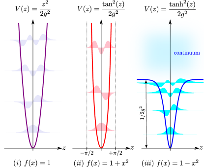
Figure 1: Potentials appearing in the eigenvalue equation (7b) for various choices of $f$. We take $g=0.225$. Note that the number of bound states in case (iii) is directly determined by the height of the finite potential; i.e., it is a function of $g=k/M_{\star}$.

(i) $f(x)=1$.

This case is the conventional quantization with $[\hat{\phi}_{\mathbf{k}},\hat{\pi}_{\mathbf{k}}]=i$; the potential in the Schrödinger equation (Fig. 1 is that of the simple harmonic oscillator. Hence,

$$\Delta E_{n}^{\mathbf{k}}=nk,\quad\langle 0_{\mathbf{k}}|\hat{\phi}_{\mathbf{k}}|n_{\mathbf{k}}\rangle=(2k)^{-1/2}\delta_{n,1}.$$ (12)

This gives the usual answer for the Green’s function

$$G(\omega,\mathbf{k})=-i/(-\omega^{2}+k^{2}).$$ (13)

We emphasize two key features responsible for the emergence of Lorentz invariance in the final step: (i) the exact cancellation of $k$ factors in the numerator of Eq. (11b), and (ii) the fact that in standard quantization, $\Delta E_{1}^{\mathbf{k}}=k$, which gives the combination $-\omega^{2}+k^{2}$ in the denominator. This provides a curious connection between the simple harmonic oscillator and Lorentz invariance, which does not exist for the potentials associated with the deformed commutator.

(ii) $f(x)=1+x^{2}$.

This form is motivated by including the gravitational interaction in discussions of the Heisenberg microscope gedanken experiments Mead (1964). It has been widely studied at the quantum mechanics level, see eg. Das and Vagenas (2008), but not in QFT. The commutator algebra is of the form (1) with $\beta>0$. The potential in the Schrödinger equation (7b) is $V(z)=\tan^{2}(z)/2g^{2}$, and is plotted in Fig. 1. The change of variables introduced in obtaining (7b) implies that the Hilbert space for this case is $L^{2}([-\pi/2,\pi/2],dz)$. The solution of the eigenvalue problem can be written down analytically in terms of hypergeometric functions Kempf et al. (1995) or Gegenbauer polynomials. The energy eigenvalues yield

$$\frac{\Delta E^{\mathbf{k}}_{n}}{k}=\left(\frac{g}{2}+\sqrt{1+\frac{g^{2}}{4}}\right)n+\frac{g}{2}n^{2}.$$ (14)

We have obtained analytic expressions for $c_{n}(\mathbf{k})$, which are plotted in Fig. 2. Note that $c_{2n}=0$ for all $g$ due to parity. The nonzero matrix elements have the following limiting behaviour

$$|c_{2n-1}|^{2}\approx\frac{1}{M_{\star}}\begin{cases}\displaystyle\frac{4\Gamma^{3}(n+1/2)g^{2n-3}}{\pi^{3/2}(2n-1)^{2}\Gamma(n)},&g\ll 1,\\ \displaystyle\frac{64n^{2}}{\pi^{2}\left(4n^{2}-1\right)^{2}},&g\gg 1.\end{cases}$$ (15)

From this formula or Fig. 2, we see that for small $g$, the first matrix element coincides with the $f(x)=1$ result $|c_{1}|^{2}=(2k)^{-1}$. The higher $n$ contributions are suppressed by successive powers of $g^{2}$, therefore the sums in (11) are dominated by the first term. Since $\Delta E_{n}^{\mathbf{k}}\approx nk$ in this regime, the propagator (13) is recovered for $k\ll M_{\star}$.

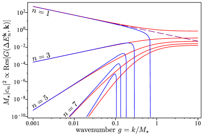
Figure 2: Matrix elements $M_{\star}|c_{n}|^{2}$ for $f=1+x^{2}$ (red), $f=1-x^{2}$ (blue), and $f=1$ (purple dashed). These are proportional to the residues associated with the resonant poles of the Green’s function.

For $g\gtrsim 1$, the $n>1$ terms in (11) cannot be neglected; each of these contributes a pair of poles at $\omega=\pm\Delta E_{n}^{\mathbf{k}}$ to the Green’s function $G(\omega,\mathbf{k})$ as depicted in Fig. 3. These poles may be interpreted as discrete resonant modes with dispersion relation $\omega^{2}=(\Delta E_{n}^{\mathbf{k}})^{2}$. Since the residues of the $n=1$ poles are always greater than those for $n>1$, we call it the “principal resonance”; its dispersion relation is shown in Fig. 4.

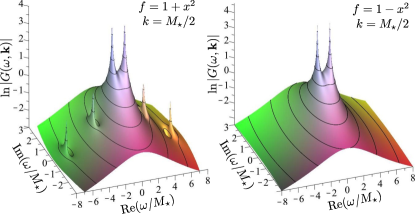
Figure 3: Bound state contributions to the Green’s function in the complex $\omega$ plane for $f=1\pm x^{2}$. Each pair of spikes indicates a resonant mode. The $f=1-x^{2}$ case has only two bounds states for this choice of parameters, and hence exhibits fewer poles than the $f=1+x^{2}$ case.

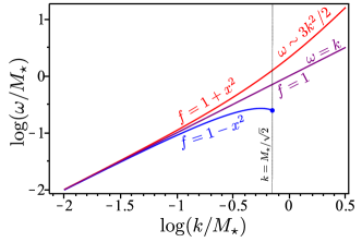
Figure 4: Dispersion relations for the principal $n=1$ resonance of $G(\omega,\mathbf{k}$) for various choices of $f$. Note that for the $f=1-x^{2}$ case, the $n=1$ bound state transitions to the continuum at $k=M_{\star}/\sqrt{2}$; hence the termination of the $\omega=\omega(k)$ curve. Dispersion relations for the higher order excitations are qualitatively similar.

Finally, we note that for $g\gg 1$, the Green’s function reduces to

$$G(\omega,\mathbf{k})\approx\frac{i}{M_{\star}}\sum_{n=1}^{\infty}\alpha_{n}\left(\frac{1}{\omega-\frac{k^{2}}{2m^{\text{eff}}_{n}}}-\frac{1}{\omega+\frac{k^{2}}{2m^{\text{eff}}_{n}}}\right),$$ (16)

with $\alpha_{n}={64n^{2}}/{\pi^{2}(4n^{2}-1)^{2}}$ and $m_{n}^{\text{eff}}={M_{\star}}/(4n^{2}-1)$. The terms in brackets are the Fourier-space propagators of the non-relativistic Schrödinger equation for a free particle of mass $m^{\text{eff}}_{n}$. This result is a curious surprise: the small wavelength limit of the propagator exhibits the Galilean symmetry of Newtonian mechanics, and indicates non-locality in space in this regime. The positive and negative energy poles reflect the fact that this comes from a relativistic theory in the long wavelength limit.

(iii) $f(x)=1-x^{2}.$

The commutator algebra in this case is of the form (1) with $\beta<0$. The potential appearing in the Schrödinger equation (7b) is $V(z)=\tanh^{2}(z)/2g^{2}$ which is a vertical translation of the well-known Pöschl-Teller potential $V(z)=-\frac{1}{2}j(j+1)\text{sech}^{2}(z)$, but with arbitrary amplitude (see eg. Arias et al. (2004)). The eigenvalue problem is again analytically solvable. However, there is a crucial difference between this case and the previous two: the fact that $V(z)$ has a finite height implies that for any given value of $g=k/M_{\star}$, there is a finite number of normalizable energy eigenstates in $L^{2}(\mathbb{R},dz)$. These states are labelled by integers $n=0\ldots n_{\text{max}}$, where $n_{\rm max}=\text{floor}[(\sqrt{4+g^{2}}-g)/2g]$. The energy differences $\Delta E_{n}^{\mathbf{k}}$ for this case are given by (14) if we substitute $g\mapsto-g$. There are no normalizable eigenstates in $L^{2}(\mathbb{R},dz)$ with energy greater than $E_{\text{max}}=M_{\star}/2$.

Because of their finite number, energy eigenfunctions do not form a complete basis of $L^{2}(\mathbb{R},dz)$ and the formulae (11) are not directly applicable. However, there is a complete energy eigenfunction basis if we instead use the Hilbert space $L^{2}([-\ell,\ell],dz)$. With this choice, the “scattering” energy eigenstates with $E>M_{\star}/2$ are normalizable and discrete, and the sums in (11) are well-defined. Taking the $\ell\rightarrow\infty$ limit, the scattering states approach a continuum and the Green’s function is

$$G(\omega,\mathbf{k})=-2i\sum_{n=1}^{n_{\text{max}}}\frac{\Delta E_{n}^{\mathbf{k}}\ |c_{n}|^{2}}{-\omega^{2}+(\Delta E_{n}^{\mathbf{k}})^{2}}\\ -\frac{i}{\pi}\int_{0}^{\infty}d\nu\frac{\Delta E_{\mathbf{k}}(\nu)|c(\nu)|^{2}}{-\omega^{2}+\Delta E_{\mathbf{k}}^{2}(\nu)}.$$ (17)

The integration is over the scattering states, which are labelled by the continuous parameter $\nu$. The energy of a given scattering state is

$$E_{\mathbf{k}}(\nu)=\frac{M_{\star}}{2}(\nu^{2}g^{2}+1),\quad\Delta E_{\mathbf{k}}(\nu)=E_{\mathbf{k}}(\nu)-E_{0}^{\mathbf{k}}.$$ (18)

Also, $c(\nu)=\lim_{\ell\rightarrow\infty}\langle\nu_{\mathbf{k}}|\hat{\phi}_{\mathbf{k}}|0_{\mathbf{k}}\rangle$ where $|\nu_{\mathbf{k}}\rangle$ is an odd-parity scattering mode of energy $E_{\mathbf{k}}(\nu)$ with normalization $\langle\nu_{\mathbf{k}}|\nu_{\mathbf{k}}\rangle=2\ell$. (Even parity modes do not contribute by symmetry.)

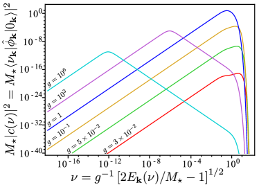
Figure 5: Scattering to bound state matrix elements $|c(\nu)|^{2}$ for the $f(x)=1-x^{2}$ case.

We have computed closed form expressions for both $|c_{n}|^{2}$ (plotted in Fig. 2) and $|c(\nu)|^{2}$ (plotted in Fig. 5). At small $g$, the bound state residues match those for the $f(x)=1+x^{2}$ case, as do the energy differences $\Delta E_{n}^{\mathbf{k}}$. Furthermore, we find $|c(\nu)|\rightarrow 0$ as $g\rightarrow 0$, which guarantees that (13) is recovered for long wavelengths.

Unlike the previous case, the bound state matrix elements go to zero for finite $g$. In fact, for $g\geq 1/\sqrt{n(n+1)}$ we have $c_{n}=0$. The vanishing of $c_{n}$ at particular values of $g=k/M_{\star}$ indicates the threshold where the $n^{\text{th}}$ eigenstate swtiches from a bound to scattering state, or vice versa. It follows that for $g\geq 1/\sqrt{2}$, the only non-zero contribution to Green’s function (17) is from the continuum integral. For $g\gg 1$, it can be shown that

$$D_{\mathbf{k}}(\tau)\approx\frac{8\sqrt{2\pi}e^{-i(M_{\star}^{3}\tau/2k^{2}+3\pi/4)}}{k(M_{\star}\tau)^{3/2}}F\left(\frac{\tau M_{\star}^{3}}{k^{2}}\right),$$ (19)

where $F(u)=1+\mathcal{O}(1/u)$ is a non-oscillatory expression involving error functions. The $\tau^{3/2}$ factor in the denominator implies that short wavelength modes decay to zero with characteristic timescale $M_{\star}^{-1}$, and the argument of the exponential gives an effective dispersion relation $\omega=M_{\star}^{3}/2k^{2}$. That is, disturbances of physical size $\ll M_{\star}^{-1}$ will not generate any long distance wave propagation in this model. It is interesting that some of the features of the $f(x)=1-x^{2}$ case appear to naturally incorporate recent ideas on the ultraviolet completion of non-renormalizable theories via a so-called “classicalization” Dvali and Gomez (2010), where propagating quantum degrees of freedom do not exist at short distance scales.

Discussion

We have shown that if modified canonical commutators are directly implemented in $\mathbf{k}$ space, the resulting QFTs exhibit novel short wavelength behaviour: propagation amplitudes have multiple poles, Lorentz invariance is broken, and there is spatial non-locality.

The expression for the propagator Eq. (11b) resembles the Lehmann-Kallen spectral representation for an interacting Lorentz invariant scalar field theory of mass $m$,

$$-iG(\omega,\mathbf{k})=\frac{1}{-\omega^{2}+\mathbf{k}^{2}+m^{2}}+\int\limits_{4m^{2}}^{\infty}\frac{d\mu^{2}\;\rho(\mu^{2})}{-\omega^{2}+\mathbf{k}^{2}+\mu^{2}},$$ (20)

where $\rho(\mu^{2})$ is the density of particle resonances of mass $\mu$. Although purely mathematical, this analogy suggests a multi-particle nature of deformed quantization, even for a free theory. (Our result on multiple poles support an argument to that effect in Hossenfelder (2008) for QFTs with a minimal length scale based on higher derivative theories.)

Another interesting outcome of this work is an explicit non-locality in space at short distance scales. This may be seen in at least two distinct ways. One is simply due to Lorentz violation; in the large $k$ regime for the case $f=1+x^{2}$, the non-localilty is exactly Newtonian action-at a-distance, as evident from the form of the propagator. The other follows directly from inverse Fourier transformation of the deformed $\mathbf{k}$ space commutator, which would lead to non-local terms of the form $M^{-1}_{\star}\int d^{3}\mathbf{z}\,\hat{\pi}(t,\mathbf{y}-\mathbf{z})\,\hat{\pi}(t,\mathbf{z})$ in the equal time commutator $[\hat{\phi}(t,\mathbf{x}),\hat{\pi}(t,\mathbf{x}+\mathbf{y})]$. The Heisenberg equations of motion derived from this commutator would be non-local integro-differential equations.

The above observation appears to resonate with the recently proposed hypothesis of relative non-locality Amelino-Camelia et al. (2011), in which locality in a postulated curved momentum space leads to non-locality in physical space. In our approach, space non-locality is evident in the above commutator, and the “relative” part may be connected with the fact that our quantization depends on a choice of time coordinate. Since that hypothesis is motivated by earlier works on deformed Lorentz symmetry, perhaps such a connection is not unexpected, with the caveat that in our approach it arises at the level of a dynamical quantum field, rather than at the kinematical level in Amelino-Camelia et al. (2011).

There are several directions for further work using the deformed quantization we have discussed. It is apparent that the approach may be followed for other spin fields in flat space time. Of particular interest is the scalar field on a black hole background; for example, modified dispersion relations of the type computed for the $f_{-}$ case, with vanishing group velocity for short wavelength modes, have been used to study Hawking radiation Unruh (1995).

For interacting theories, perhaps of most interest for observational consequences is quantum electrodynamics. Of related interest is whether Lorentz violation from this type of deformed quantization gives rise to order one effects due to loop corrections, as discussed in the context of effective field theory (EFT) in Collins et al. (2004). However, many components of conventional quantization are prima-facie absent in our deformed quantization, so it is not clear whether the axioms of EFT apply. Indeed, space non-locality at short wavelengths appears to complicate the Wilsonian program of integrating out high energy degrees of freedom and capturing their effects in local counter-term; related comments on this appear in Dvali and Gomez (2010). Thus, any arguments on Lorentz violation based on EFT would have to be carefully reformulated before making statements concerning renormalization and loop corrections.

This work was supported by an Atlantic Association for Research in the Mathematical Sciences (AARMS) post-doctoral fellowship (D.K.) and NSERC of Canada.

References

- Kempf et al. (1995) A. Kempf, G. Mangano, and R. B. Mann, Phys.Rev. D52, 1108 (1995), eprint hep-th/9412167.
- Hassan and Sloth (2003) S. Hassan and M. S. Sloth, Nucl.Phys. B674, 434 (2003), eprint hep-th/0204110.
- Pikovski et al. (2012) I. Pikovski, M. R. Vanner, M. Aspelmeyer, M. Kim, C. Brukner, et al., Nature Phys. 8, 393 (2012), eprint 1111.1979.
- Hossain et al. (2010) G. M. Hossain, V. Husain, and S. S. Seahra, Phys.Rev. D82, 124032 (2010), eprint 1007.5500.
- Husain and Kreienbuehl (2010) V. Husain and A. Kreienbuehl, Phys. Rev. D81, 084043 (2010), eprint 1002.0138.
- Mead (1964) C. A. Mead, Phys. Rev. 135, 849 (1964).
- Das and Vagenas (2008) S. Das and E. C. Vagenas, Phys.Rev.Lett. 101, 221301 (2008), eprint 0810.5333.
- Arias et al. (2004) J. Arias, J. Gomez-Camacho, and R. Lemus, J.Phys.A A37, 877 (2004).
- Dvali and Gomez (2010) G. Dvali and C. Gomez (2010), eprint 1005.3497.
- Hossenfelder (2008) S. Hossenfelder, Class.Quant.Grav. 25, 038003 (2008), eprint 0712.2811.
- Amelino-Camelia et al. (2011) G. Amelino-Camelia, L. Freidel, J. Kowalski-Glikman, and L. Smolin, Phys.Rev. D84, 084010 (2011), eprint 1101.0931.
- Unruh (1995) W. Unruh, Phys.Rev. D51, 2827 (1995).
- Collins et al. (2004) J. Collins, A. Perez, D. Sudarsky, L. Urrutia, and H. Vucetich, Phys.Rev.Lett. 93, 191301 (2004), eprint gr-qc/0403053.