Dilepton production in pion–nucleon collisions in an effective field theory approach

Abstract

We present a model of electron-positron pair production in pion-nucleon collisions in the exclusive reaction $\pi N\rightarrow Ne^{+}e^{-}$. The model is based on an effective field theory approach, incorporating 16 baryon resonances below 2 GeV. Parameters of the model are fitted to pion photoproduction data. We present the resulting dilepton invariant mass spectra for $\pi^{-}p$ collisions up to $\sqrt{s}=1.9$ GeV center-of-mass collision energy. These results are meant to give predictions for the planned experiments at the HADES spectrometer in GSI, Darmstadt.

I Introduction

Dileptons are among the most important signals studied in heavy ion collision experiments. In the 1–2 GeV/nucleon energy range electron-positron pair production has been studied by the DiLepton Spectrometer (DLS) at LBL and, more recently, by the High Acceptance Di-Electron Spectrometer (HADES) at GSI. Due to the high complexity of nuclear collision processes, the experimental results can be interpreted only via comparison with model calculations. Usually transport models are used for this purpose. These models need the cross sections of elementary hadronic collisions as input, therefore a good understanding of the elementary cross sections is essential.

Both DLS DLS_NN and HADES HADES_NN studied dilepton production in elementary $NN$ collisions. In parallel a lot of theoretical work has been done in order to achieve a good description of the experimental dilepton spectrum. Earlier, a resonance approach was used Wolf_dilep ; Bratkovskaya , where particle production is described as a multistep process. In the first step a baryon resonance is created which then decays in one or more steps, creating the final state particles, including dileptons. This approach naturally fits the particle production mechanism of transport codes. Recent calculations apply one-boson-exchange effective Lagrangians to calculate the $NN\rightarrow NNe^{+}e^{-}$ cross section Shyam2003 ; Kaptari2006 ; Kaptari2007 ; Shyam2009 ; Kaptari2009 ; Shyam2010 . Although a lot of progress has been made, the measured dilepton spectra are still not perfectly reproduced by the theoretical models Shyam2010 .

In heavy ion collisions a large number of pions are produced, therefore elementary $\pi N$ collisions are also important. Moreover, besides photon induced reactions, pion beams are much more suitable for studying individual resonances than nuclear projectiles. At HADES new experiments are planned with a pion beam, where both $\pi A$ and $\pi N$ collisions would be studied. At the same time, dilepton production in $\pi N$ collisions have not yet been studied in an effective field theory approach similar to those used in the $NN$ case.

The process $\pi N\rightarrow Ne^{+}e^{-}$ is related to the time inverse of pion photoproduction, which is the key experiment in determining the electromagnetic properties of baryon resonances, and is studied in great detail both experimentally and theoretically. In particular, effective field theory models have been used to study pion photoproduction Garcilazo ; Feuster_Mosel_NPA ; Fernandez .

In the present paper we set up a model of electron-positron pair production in $\pi N$ collisions based on an effective field theory approach.

The paper is organized as follows. In Sec. II we review the kinematics of the $\pi N\rightarrow Ne^{+}e^{-}$ process and give the expressions for the differential cross section. In Sec. III we specify the effective Lagrangians and discuss the calculation of the transition matrix elements. Separate subsections deal with the version of the vector meson dominance model used in this paper to describe the electromagnetic interaction of hadrons; the contribution of the nonresonant Feynman diagrams to the matrix element, with an emphasis on the gauge-invariance preserving scheme for hadronic form factors; the contribution of baryon resonances. For nonresonant contributions explicit analytical expressions for the matrix elements are listed, while the contributions of baryon resonances are calculated numerically.

In Sec. IV we discuss the determination of baryon resonance parameters from pion photoproduction data. The calculated dilepton spectra are shown in Sec. V, followed by a discussion.

II Kinematics

Figure 1: Schematic diagram of the process $\pi+N\rightarrow N+e^{+}+e^{-}$.

The differential cross section of the process $\pi+N\rightarrow N+e^{+}+e^{-}$ is given by

$$d\sigma=\frac{(2\pi)^{4}}{4\sqrt{(p_{i}\cdot q)^{2}-m_{N}^{2}m_{\pi}^{2}}}\frac{1}{n_{\text{pol}}}\sum_{\text{pol}}\left|\mathcal{M}\right|^{2}d\Phi_{3}\left(p_{i}+q;p_{f},k_{1},k_{2}\right),$$ (1)

where the $n$-body phase-space is defined by

$$d\Phi_{n}\left(P;p_{1},...,p_{n}\right)=\delta^{(4)}\left(P-\sum_{i=1}^{n}p_{i}\right)\prod_{i=1}^{n}\frac{d^{3}\mathbf{p}_{i}}{(2\pi)^{3}2p_{i0}},$$ (2)

and we have used the notation of Fig. 1 for the four-momenta of particles. The three-body phase-space in Eq. (1) can be calculated recursively as

$$d\Phi_{3}\left(p_{i}+q;p_{f},k_{1},k_{2}\right)=(2\pi)^{3}d(k^{2})d\Phi_{2}\left(p_{i}+q;p_{f},k\right)d\Phi_{2}\left(k;k_{1},k_{2}\right).$$ (3)

Making use of the Dirac-$\delta$ in Eq. (2) we can integrate out four of the six momentum components in the case of the two-body phase-space, to get

$$d\Phi_{2}\left(P;p_{1},p_{2}\right)=\frac{1}{4(2\pi)^{6}}\frac{|\mathbf{p}_{1}|}{\sqrt{P^{2}}}d\Omega_{1},$$ (4)

where $\mathbf{p}_{1}$ is the spatial part of $p_{1}$ in the frame where $P$ is at rest, and $d\Omega_{1}=d\phi_{1}d(\cos\theta_{1})$ is the solid angle of $p_{1}$ in the same reference frame.

Using this the differential cross section Eq. (1) can be written in the form

$$d\sigma=\frac{1}{64(2\pi)^{5}|\mathbf{q}|s}d(k^{2})d\Omega_{\mathbf{k}}d\Omega_{\mathbf{k}_{1}}\frac{|\mathbf{k}||\mathbf{k}_{1}|}{\sqrt{k^{2}}}\frac{1}{n_{\text{pol}}}\sum_{\text{pol}}\left|\mathcal{M}\right|^{2}.$$ (5)

For unpolarized beams $d\sigma$ is independent of the azimuth angle $\phi_{\mathbf{k}}$, which can be integrated out. Note that $\mathbf{k}_{1}$ and $d\Omega_{\mathbf{k}_{1}}$ is defined in the rest frame of the decaying virtual photon of momentum $k$, in accordance with Eq. (4). Further, $\sqrt{k^{2}}=M$ is the dilepton invariant mass, and $d(k^{2})=d(M^{2})=2MdM$. Neglecting the electron mass we get $|\mathbf{k}_{1}|=M/2$. The differential cross section is then

$$\frac{d\sigma}{dM}=\frac{M}{64(2\pi)^{4}s}\frac{|\mathbf{k}|}{|\mathbf{q}|}\int d(\cos\theta_{\mathbf{k}})d\Omega_{\mathbf{k}_{1}}\frac{1}{n_{\text{pol}}}\sum_{\text{pol}}\left|\mathcal{M}\right|^{2}.$$ (6)

In Eq. (6) the magnitudes of the center-of-mass momenta are given by

$$|\mathbf{q}| = \frac{\sqrt{\lambda(s,m_{N}^{2},m_{\pi}^{2})}}{2\sqrt{s}}$$ (7)

$$|\mathbf{k}| = \frac{\sqrt{\lambda(s,m_{N}^{2},M^{2})}}{2\sqrt{s}},$$ (8)

with $\lambda(a,b,c)=a^{2}+b^{2}+c^{2}-2(ab+bc+ca)$.

The leptonic part of the matrix element $\mathcal{M}$ can be written out explicitly, resulting in the expression

$$\mathcal{M}=-\frac{e}{k^{2}}\mathcal{M}_{\mu}^{\text{had}}\bar{u}(k_{1})\gamma^{\mu}v(k_{2}).$$ (9)

The squared matrix element summed over polarizations is

$$\sum_{\text{pol}}\left|\mathcal{M}\right|^{2}=\frac{e^{2}}{k^{4}}W_{\mu\nu}l^{\mu\nu},$$ (10)

with the hadronic tensor $W_{\mu\nu}$ defined by

$$W_{\mu\nu}=\sum_{\text{pol}}\mathcal{M}_{\mu}^{\text{had}}{\mathcal{M}_{\nu}^{\text{had}}}^{*},$$ (11)

and the leptonic tensor $l^{\mu\nu}$ given by

$$l^{\mu\nu}=4\left(k_{1}^{\mu}k_{2}^{\nu}+k_{1}^{\nu}k_{2}^{\mu}-(k_{1}\cdot k_{2})g^{\mu\nu}\right).$$ (12)

III Effective Lagrangians and Matrix Elements

Figure 2: Feynman diagrams contributing to the process $\pi+N\rightarrow N+e^{+}+e^{-}$.

The Feynman diagrams contributing to the process $\pi+N\rightarrow N+e^{+}+e^{-}$ are depicted in Fig. 2. These are: the Born contributions [(a) $s$-, (b) $u$-, and (c) $t$-channel diagrams, and (d) contact interaction term], (e) vector meson exchange diagram, (f) $s$-channel and (g) $u$-channel baryon resonance contributions.

III.1 Electromagnetic interaction of hadrons

In most studies the electromagnetic interaction of hadrons is described using some variant of the vector meson dominance (VMD) model VMD . Here we adopt a version of the model described in Appendix B of Ref. Kroll and also in Ref. VMD1 , where it is denoted VMD1. In this version only the $\rho^{0}$ vector meson is included and the $\rho\gamma$ coupling has the form

$$\mathcal{L}_{\rho\gamma}=-\frac{e}{2g_{\rho}}F^{\mu\nu}\rho^{0}_{\mu\nu},$$ (13)

where $F^{\mu\nu}=\partial_{\mu}A_{\nu}-\partial_{\nu}A_{\mu}$ is the electromagnetic field strength tensor and $\rho^{0}_{\mu\nu}=\partial_{\mu}\rho^{0}_{\nu}-\partial_{\nu}\rho^{0}_{\mu}$. From the width of the $\rho\rightarrow e^{+}e^{-}$ decay, the value $g_{\rho}=4.96$ is obtained.

In addition we have to specify the coupling of various hadrons to the $\rho^{0}$. Hadrons can also directly couple to the electromagnetic field $A^{\mu}$. The full electromagnetic vertex of hadrons $h_{1}$ and $h_{2}$ is, therefore, the sum of the direct photon term and the VMD contribution (see Fig. 3). The vertex function corresponding to the VMD contribution to the $h_{1}h_{2}\gamma$ coupling has the form

$$V^{\mu\ldots}_{h_{1}h_{2}\gamma,\text{VMD}}(k)=F_{\text{VMD}}(k^{2})V^{\mu\ldots}_{h_{1}h_{2}\rho}(k),$$ (14)

where the VMD form factor appearing on the right hand side is given by

$$F_{\text{VMD}}(k^{2})=-\frac{e}{g_{\rho}}\frac{k^{2}}{k^{2}-m_{\rho}^{2}+i\sqrt{k^{2}}\Gamma_{\rho}(k^{2})},$$ (15)

and is the product of the $\rho$ meson propagator and the $\rho\gamma$ vertex contribution. In Eq. (14) $k$ is the photon four-momentum, $\mu$ is the Lorentz index of the photon line and the dots stand for possible further Lorentz indices corresponding to Rarita-Schwinger fields in case $h_{1}$ or $h_{2}$ are higher spin baryons.

Figure 3: According to the vector meson dominance (VMD) model applied in this paper, the full electromagnetic vertex is a sum of the direct photon term and the $\rho$ meson contribution.

For the electromagnetic interaction of a baryon resonance $R$ ($h_{1}=R$ and $h_{2}=N$), the $g_{RN\rho}$ coupling constants can be determined from the $R\rightarrow N\rho$ width of the baryon resonance $R$. The VMD form factor in Eq. (15) is proportional to $k^{2}$, therefore the VMD part of the electromagnetic vertex does not contribute to the $R\rightarrow N\gamma$ decay width for real photons, $k^{2}=0$. Thus, $g_{RN\gamma}$ can be fixed independently using the photonic decay width $\Gamma_{R\rightarrow N\gamma}$. This is an advantage of the choice of the VMD Lagrangian Eq. (13). If instead one uses the more common form

$$\tilde{\mathcal{L}}_{\rho\gamma}=-\frac{em_{\rho}^{2}}{g_{\rho}}\rho^{0}_{\mu}A^{\mu},$$ (16)

$k^{2}$ in the numerator of the VMD form factor, Eq. (15) is replaced by $m_{\rho}^{2}$. In that case the VMD contribution to $\Gamma_{R\rightarrow N\gamma}$ is nonzero, and in fact overpredicts the physical $N\gamma$ width for most of the baryon resonances, as pointed out in Ref. Friman_Pirner .

III.2 Nonresonant contributions

III.2.1 Contributions of direct photon couplings

In order to calculate the nonresonant Feynman diagrams Fig. 2(a)–(e), we have to specify the hadronic and electromagnetic interaction Lagrangians of pions and nucleons. We use a pseudovector $NN\pi$ coupling,

$$\mathcal{L}_{NN\pi}=-\frac{f_{NN\pi}}{m_{\pi}}\bar{\psi}_{N}\gamma_{5}\gamma^{\mu}\vec{\tau}\psi_{N}\cdot\partial_{\mu}\vec{\pi}.$$ (17)

Following Ref. Garcilazo we use the value $f_{NN\pi}=0.97$ for the coupling constant.

The electromagnetic interaction Lagrangians must be chosen in such a way that electromagnetic gauge invariance is fulfilled. This will ensure that the photon field $A^{\mu}$ will couple to conserved currents constructed from the hadron fields, and the resulting hadronic matrix elements will satisfy the condition $\mathcal{M}_{\mu}^{\text{had}}k^{\mu}=0$. An important consequence is, that the photon propagator can be written as $-ig_{\mu\nu}/k^{2}$, which has been used in the derivation of Eq. 9.

Gauge invariant Lagrangians can be obtained by replacing derivatives $\partial_{\mu}$ with the covariant derivative

$$\nabla_{\mu}=\partial_{\mu}+ieA_{\mu}Q$$ (18)

in all terms of the Lagrangian ($Q$ is the electric charge operator). Carrying out this replacement in the nucleon kinetic energy term results in the $NN\gamma$ interaction Lagrangian $-e\bar{\psi}_{N}\not{A}Q\psi_{N}$. This is supplemented by the magnetic term, which contains the field tensor $F^{\mu\nu}$, and is gauge invariant. The complete $NN\gamma$ interaction is then

$$\mathcal{L}_{NN\gamma}=-e\bar{\psi}_{N}\left[\frac{1+\tau_{3}}{2}\not{A}-\left(\frac{1+\tau_{3}}{2}\kappa_{p}+\frac{1-\tau_{3}}{2}\kappa_{n}\right)\frac{\sigma_{\mu\nu}}{4m_{N}}F^{\mu\nu}\right]\psi_{N}.$$ (19)

(The isospin 1/2 representation of the electric charge operator, $Q=(1+\tau_{3})/2$ has been substituted.)

Starting from the pion kinetic energy term we obtain the $\pi\pi\gamma$ interaction in the form

$$\mathcal{L}_{\pi\pi\gamma}=-eA_{\mu}J_{\pi}^{\mu},$$ (20)

where $J_{\pi}^{\mu}=i(\pi^{-}\partial^{\mu}\pi^{+}-\pi^{+}\partial^{\mu}\pi^{-})$ is the pion current. In addition a $\pi\pi\gamma\gamma$ term is also generated, but it does not contribute to the studied process.

Inserting the covariant derivative in the pseudovector pion-nucleon coupling term we obtain an $NN\pi\gamma$ contact interaction of the form

$$\mathcal{L}_{NN\pi\gamma}=-\frac{ief_{NN\pi}}{m_{\pi}}\bar{\psi}_{N}\gamma_{5}\gamma^{\mu}\vec{\tau}\psi\cdot A_{\mu}Q\vec{\pi}.$$ (21)

Using the Lagrangians Eqs. (17),(19)–(21) we can calculate those Born contributions [diagrams (a)–(d) in Fig. 2] to $\mathcal{M}_{\mu}^{\text{had}}$ that contain a direct photon coupling. The construction of the Lagrangians assures that the sum of these contributions satisfies the gauge invariance condition $\mathcal{M}_{\mu}^{\text{had}}k^{\mu}=0$. Note, however, that the individual Feynman diagrams are not gauge invariant.

In order to describe the off-shell behavior of internal hadron lines we apply at all hadronic vertices form factors given by

$$F_{1}(s) = \frac{1}{1+(s-m_{N}^{2})^{2}/\Lambda^{4}},$$ (22)

$$F_{2}(u) = \frac{1}{1+(u-m_{N}^{2})^{2}/\Lambda^{4}},$$ (23)

$$F_{3}(t) = \frac{1}{1+(t-m_{\pi}^{2})^{2}/\Lambda^{4}}$$ (24)

for $s$-, $u$- and $t$-channel diagrams, respectively. These satisfy

$$F_{1}(m_{N}^{2})=F_{2}(m_{N}^{2})=F_{3}(m_{\pi}^{2})=1.$$ (25)

The application of different form factors to the individual diagrams Fig. 2(a)–(c) destroys the overall gauge invariance of the Born contributions. The solution to this problem has been given by Davidson and Workman in the case of pion photoproduction Davidson-Workman , and the method can be generalized to the present case. We first write $\mathcal{M}_{\mu}^{\text{had}}$ in the form

$$\mathcal{M}_{\mu}^{\text{had}}=\bar{u}_{f}T_{\mu}u_{i}.$$ (26)

Let $T_{\mu}^{\text{Born}}$ denote the Born contribution to $T_{\mu}$ obtained from direct photon terms. It can be shown by explicit calculation of $T_{\mu}^{\text{Born}}$ from the Born channel Feynman diagrams, that the replacement $T_{\mu}^{\text{Born}}\rightarrow T_{\mu}^{\text{Born}}+\Delta T_{\mu}^{\text{Born}}$ makes the hadronic matrix element $\mathcal{M}_{\mu}^{\text{had}}$ gauge invariant, if

$$\Delta T_{\mu}^{\text{Born}}=\frac{\sqrt{2}ef_{NN\pi}}{m_{\pi}}2m_{N}\gamma_{5}\left[\left(\hat{F}(s,u,t)-F_{3}(t)\right)\frac{2q^{\mu}-k^{\mu}}{t-m_{\pi}^{2}}-\left(\hat{F}(s,u,t)-F_{2}(u)\right)\frac{2p_{i}^{\mu}-k^{\mu}}{u-m_{N}^{2}}\right],$$ (27)

where

$$\hat{F}(s,u,t)=F_{1}(s)+F_{2}(u)+F_{3}(t)-F_{1}(s)F_{2}(u)-F_{1}(s)F_{3}(t)-F_{2}(u)F_{3}(t)+F_{1}(s)F_{2}(u)F_{3}(t).$$ (28)

$\hat{F}(s,u,t)$ was chosen in such a way that

$$\hat{F}(m_{N}^{2},u,t)=\hat{F}(s,m_{N}^{2},t)=\hat{F}(s,u,m_{\pi}^{2})=1,$$ (29)

which means that the poles of $T_{\mu}^{\text{Born}}$ at $t=m_{\pi}^{2}$ and $u=m_{N}^{2}$ are canceled by the factors $\hat{F}-F_{2(3)}$. This means that the term $\Delta T_{\mu}^{\text{Born}}$ can be generated by adding a suitably chosen contact interaction to the Lagrangian.

Gauge invariance of the resulting $T_{\mu}^{\text{Born}}$ can be made transparent by writing it in the form

$$T_{\mu}^{\text{Born}}=\sum_{i=1}^{4}A_{i}M_{i,\mu},$$ (30)

where $M_{i,\mu}$ denote the gauge invariant combinations

$$M_{1,\mu} = \gamma_{5}\left(\gamma_{\mu}\not{k}-k_{\mu}\right),$$ (31)

$$M_{2,\mu} = \frac{\gamma_{5}}{2}\left[(2p_{i\mu}-k_{\mu})(2q\cdot k-M^{2})-(2q_{\mu}-k_{\mu})(2p_{i}\cdot k-M^{2})\right],$$ (32)

$$M_{3,\mu} = \frac{\gamma_{5}}{2}\left[\gamma_{\mu}(2p_{f}\cdot k+M^{2})-(2p_{f\mu}+k_{\mu})\not{k}\right],$$ (33)

$$M_{4,\mu} = \frac{\gamma_{5}}{2}\left[\gamma_{\mu}(2p_{i}\cdot k-M^{2})-(2p_{i\mu}-k_{\mu})\not{k}\right].$$ (34)

In the $k^{2}=0$ limit $M_{i,\mu}$ correspond to the gauge invariant combinations defined in Ref. Davidson-Workman for the case of pion photoproduction.

The coefficients $A_{i}$ are obtained from the explicit Feynman diagram calculations and are given by

$$A_{1} = -\frac{\sqrt{2}ef_{NN\pi}}{m_{\pi}}\left[\frac{1}{2m_{N}}\left(F_{1}\kappa_{n}+F_{2}\kappa_{p}\right)+\frac{2m_{N}F_{2}}{u-m_{N}^{2}}(1+\kappa_{p})+\frac{2m_{N}F_{1}}{s+m_{N}^{2}}\kappa_{n}\right],$$ (35)

$$A_{2} = \frac{\sqrt{2}ef_{NN\pi}}{m_{\pi}}\frac{4m_{N}\hat{F}}{(t-m_{\pi}^{2})(u-m_{N}^{2})},$$ (36)

$$A_{3} = \frac{\sqrt{2}ef_{NN\pi}}{m_{\pi}}\frac{2\kappa_{n}F_{1}}{s-m_{N}^{2}},$$ (37)

$$A_{4} = \frac{\sqrt{2}ef_{NN\pi}}{m_{\pi}}\frac{2\kappa_{p}F_{2}}{u-m_{N}^{2}}.$$ (38)

In the derivation of Eqs. (35)–(38) we have used the fact, that $k_{\mu}l^{\mu\nu}=0$, and thus arbitrary terms proportional to $k_{\mu}$ can be added to $T_{\mu}$ without affecting the cross section.

III.2.2 VMD contributions to Born diagrams

For the calculation of the VMD contributions we need the coupling of hadrons to the $\rho^{0}$ meson. Here we face the same problems related to gauge invariance as in the case of the direct photon couplings. First we have to ensure that the relation $\mathcal{M}_{\mu}^{\text{had}}k^{\mu}=0$ holds without the inclusion of hadronic form factors. One possibility to fulfill this condition is to define the interaction of $\rho$ mesons with other hadrons by replacing derivatives $\partial_{\mu}$ in the hadronic Lagrangians with

$$\nabla_{\mu}=\partial_{\mu}-i\tilde{g}_{\rho}\vec{\rho}_{\mu}\cdot\vec{T},$$ (39)

where $\vec{T}$ denotes the generators of the isospin SU(2) group. This method is inspired by an SU(2) gauge theory with $\rho$ mesons as gauge bosons.

In this way an $NN\rho$ interaction term can be obtained from the nucleon kinetic energy term. Similarly to the direct photon coupling, a magnetic type term can be added to it, yielding the total $NN\rho$ interaction Lagrangian

$$\mathcal{L}_{NN\rho}=\frac{\tilde{g}_{\rho}}{2}\bar{\psi}_{N}\left(\vec{\not{\rho}}-\kappa_{\rho}\frac{\sigma_{\mu\nu}}{4m_{N}}\vec{\rho}^{\mu\nu}\right)\cdot\vec{\tau}\psi_{N}.$$ (40)

The $\rho\pi\pi$ term is obtained from the pion kinetic energy term and has the form

$$\mathcal{L}_{\rho\pi\pi}=-\tilde{g}_{\rho}\left[(\partial^{\mu}\vec{\pi})\times\vec{\pi}\right]\cdot\vec{\rho}_{\mu}.$$ (41)

Comparing the Lagrangians Eqs. (40) and (41) with the traditional forms of the $NN\rho$ and $\rho\pi\pi$ couplings, we see that their construction in terms of the covariant derivative Eq. (39) provides a relation of their coupling constants in the form

$$2g_{NN\rho}=g_{\rho\pi\pi}=\tilde{g}_{\rho}.$$ (42)

From the width of the decay $\rho\rightarrow\pi\pi$ the value $g_{\rho\pi\pi}=5.96$ is obtained. $g_{NN\rho}$ can be determined from low energy nucleon-nucleon scattering. In Ref. Fernandez the value $g_{NN\rho}=2.6$ was used, yielding the ratio $g_{\rho\pi\pi}/g_{NN\rho}=2.29$, which is reasonably close to the value of 2 predicted by SU(2) gauge invariance. In the present calculation we use the values $\tilde{g}_{\rho}=g_{\rho\pi\pi}=5.96$ and $g_{NN\rho}=\tilde{g}_{\rho}/2=2.98$.

Inserting the covariant derivative Eq. (39) in the pseudovector $NN\pi$ Lagrangian Eq. (17) we obtain an $NN\pi\rho$ contact interaction,

$$\mathcal{L}_{NN\pi\rho}=-\frac{\tilde{g}_{\rho}f_{NN\pi}}{m_{\pi}}\bar{\psi}_{N}\gamma_{5}\gamma^{\mu}\vec{\tau}\psi\cdot\left(\vec{\rho}_{\mu}\times\vec{\pi}\right).$$ (43)

In accordance with Eq. (14) the VMD contribution to the hadronic matrix element can be written in the form

$$\mathcal{M}_{\mu}^{\text{had,VMD}}=F_{\text{VMD}}(k^{2})\tilde{\mathcal{M}}_{\mu},$$ (44)

where the VMD form factor $F_{\text{VMD}}(k^{2})$ is given by Eq. (15). Feynman diagrams representing $\tilde{\mathcal{M}}_{\mu}$ can be obtained from the VMD diagrams by truncating the dilepton part, starting from the $\rho$ propagator.

At hadronic vertices we employ the same form factors [Eqs. (22)–(24)] as in the direct photon contributions. Then we write $\tilde{\mathcal{M}}_{\mu}$ in the form

$$\tilde{\mathcal{M}}_{\mu}=\bar{u}_{f}\tilde{T}_{\mu}u_{i}.$$ (45)

The explicit form of $\tilde{T}_{\mu}^{\text{Born,VMD}}$ (the contribution to $\tilde{T}_{\mu}$ of Born diagrams with VMD coupling) is calculated from the relevant Feynman diagrams. We observe that the replacement $\tilde{T}_{\mu}^{\text{Born,VMD}}\rightarrow\tilde{T}_{\mu}^{\text{Born,VMD}}+\Delta\tilde{T}_{\mu}^{\text{Born,VMD}}$ ensures the validity of the gauge invariance relation, $\mathcal{M}_{\mu}^{\text{had,VMD}}k^{\mu}=0$ if $\Delta\tilde{T}_{\mu}^{\text{Born,VMD}}$ is chosen as

$$\Delta\tilde{T}_{\mu}^{\text{Born,VMD}}=\frac{\tilde{g}_{\rho}f_{NN\pi}}{\sqrt{2}m_{\pi}}2m_{N}\gamma_{5}$$ (47)

$$\times\left[\left(\hat{F}(s,u,t)-F_{2}(u)\right)\frac{2p_{i}^{\mu}-k^{\mu}}{u-m_{N}^{2}}-\left(\hat{F}(s,u,t)-F_{1}(u)\right)\frac{2p_{f}^{\mu}+k^{\mu}}{s-m_{N}^{2}}-2\left(\hat{F}(s,u,t)-F_{3}(t)\right)\frac{2q^{\mu}-k^{\mu}}{t-m_{\pi}^{2}}\right].$$

This $\Delta\tilde{T}_{\mu}^{\text{Born,VMD}}$ is free from poles, and is assumed to be generated by suitable contact terms added to the Lagrangian.

The obtained $\tilde{T}_{\mu}^{\text{Born,VMD}}$ can be expanded as

$$\tilde{T}_{\mu}^{\text{Born,VMD}}=\sum_{i=1}^{5}\tilde{A}_{i}M_{i,\mu},$$ (48)

where $M_{1...4,\mu}$ are given in Eqs. (31)–(34), and

$$M_{5,\mu}=\frac{\gamma_{5}}{2}\left[(2p_{f\mu}+k_{\mu})(2q\cdot k-M^{2})-(2q_{\mu}-k_{\mu})(2p_{f}\cdot k+M^{2})\right].$$ (49)

The coefficients $\tilde{A}_{i}$ are obtained as

$$\tilde{A}_{1} = \frac{\tilde{g}_{\rho}f_{NN\pi}}{\sqrt{2}m_{\pi}}\left[\frac{\kappa_{\rho}}{2m_{N}}\left(F_{2}-F_{1}\right)+2m_{N}(1+\kappa_{\rho})\left(\frac{F_{2}}{u-m_{N}^{2}}-\frac{F_{1}}{s-m_{N}^{2}}\right)\right],$$ (50)

$$\tilde{A}_{2} = -\frac{\tilde{g}_{\rho}f_{NN\pi}}{\sqrt{2}m_{\pi}}\frac{4m_{N}\hat{F}}{(t-m_{\pi}^{2})(u-m_{N}^{2})},$$ (51)

$$\tilde{A}_{3} = \frac{\tilde{g}_{\rho}f_{NN\pi}}{\sqrt{2}m_{\pi}}\frac{2\kappa_{\rho}F_{1}}{s-m_{N}^{2}},$$ (52)

$$\tilde{A}_{4} = -\frac{\tilde{g}_{\rho}f_{NN\pi}}{\sqrt{2}m_{\pi}}\frac{2\kappa_{\rho}F_{2}}{u-m_{N}^{2}},$$ (53)

$$\tilde{A}_{5} = -\frac{\tilde{g}_{\rho}f_{NN\pi}}{\sqrt{2}m_{\pi}}\frac{4m_{N}\hat{F}}{(t-m_{\pi}^{2})(s-m_{N}^{2})}.$$ (54)

III.2.3 $t$-channel $\rho$- and $a_{1}$-exchange contributions

We also calculated the contributions of the $t$-channel $\rho$- and $a_{1}$-exchange diagrams, Fig. 2(e). For the $\rho$ exchange we adopt the $\rho\pi\gamma$ interaction Lagrangian from Ref. Feuster_Mosel_NPA ,

$$\mathcal{L}_{\rho\pi\gamma}=e\frac{g_{\rho\pi\gamma}}{4m_{\pi}}\epsilon_{\mu\nu\lambda\sigma}F^{\mu\nu}\vec{\rho}^{\lambda\sigma}\cdot\vec{\pi}.$$ (55)

The value of the coupling constant, $g_{\rho\pi\gamma}=0.103$, is obtained from the width of the $\rho\rightarrow\pi\gamma$ decay. Lagrangians equivalent to the above $\mathcal{L}_{\rho\pi\gamma}$ have been used in Refs. Fernandez ; Garcilazo .

The $a_{1}\pi\gamma$ interaction was studied in Ref. Xiong . In that paper the momentum space form of the interaction Lagrangian was given. Its coordinate space equivalent is given by

$$\mathcal{L}_{a_{1}\pi\gamma}=-ie\frac{g_{a_{1}\pi\gamma}}{m_{\pi}}\vec{a}_{\mu}F^{\mu\nu}\cdot\partial_{\nu}\vec{\pi},$$ (56)

where $\vec{a}_{\mu}$ denotes the axial-vector–isovector $a_{1}$ field. From the width of the $a_{1}\rightarrow\pi\gamma$ decay we get $g_{a_{1}\pi\gamma}=0.106$ for the coupling constant.

We also need to specify the form of the $NNa_{1}$ interaction. The role of $t$-channel $a_{1}$ exchange in the nucleon-nucleon interaction was studied in Ref. Durso . They take the $NNa_{1}$ Lagrangian from the chiral $SU(2)\times SU(2)$ model of Ref. Wess-Zumino . In that model the Lagrangian has the form

$$\mathcal{L}_{NNa_{1}}=g_{NNa_{1}}\bar{\psi}_{N}\gamma^{\mu}\gamma_{5}\vec{\tau}\psi_{N}\cdot\vec{a_{\mu}},$$ (57)

and the coupling constant is related to the pseudovector pion-nucleon coupling via

$$\frac{g_{NNa_{1}}}{m_{a_{1}}}=\frac{f_{NN\pi}}{m_{\pi}}.$$ (58)

This relation gives the value $g_{NNa_{1}}=8.65$. In Ref. Yu the nucleon-$a_{1}$ coupling has been determined from the nucleon axial form factor, and the value $g_{NNa_{1}}=6.7$ was obtained.

In close analogy with the Born contributions we apply form factors given by

$$F_{V}(t)=\frac{1}{1+(t-m_{V}^{2})^{2}/\Lambda^{4}}$$ (59)

for $t$-channel $\rho$- and $a_{1}$-exchange diagrams, where $m_{V}$ denotes the $\rho$ or $a_{1}$ meson mass.

We found that the contribution of $t$-channel $\rho$ exchange is at least three orders of magnitude smaller than the Born contribution in the $\sqrt{s}\leq 1$GeV energy range. The $a_{1}$-exchange contribution is even smaller and never exceeds 10% of the $\rho$ contribution.

III.3 Contributions of baryon resonances

III.3.1 Interaction Lagrangians

In order to calculate the $s$- and $u$-channel baryon resonance contributions, diagrams Fig. 2(f) and (g), we have to specify the coupling of baryon resonances to the $\pi N$, $\rho N$ and $\gamma N$ channels.

Similarly to the nucleon-pion interaction we employ pseudovector couplings in the case of spin-1/2 nucleon resonances,

$$\mathcal{L}_{R_{1/2}N\pi}=-\frac{g_{RN\pi}}{m_{\pi}}\bar{\psi}_{R}\Gamma\gamma^{\mu}\vec{\tau}\psi_{N}\cdot\partial_{\mu}\vec{\pi}+\text{H.c.}$$ (60)

In the spin-3/2 case we use the Lagrangian

$$\mathcal{L}_{R_{3/2}N\pi}=\frac{g_{RN\pi}}{m_{\pi}}\bar{\psi}_{R}^{\mu}\Gamma\vec{\tau}\psi_{N}\cdot\partial_{\mu}\vec{\pi}+\text{H.c.},$$ (61)

while in the spin-5/2 case the Lagrangian

$$\mathcal{L}_{R_{5/2}N\pi}=\frac{g_{RN\pi}}{m_{\pi}}\bar{\psi}_{R}^{\mu\nu}\Gamma\vec{\tau}\psi_{N}\cdot\partial_{\mu}\partial_{\nu}\vec{\pi}+\text{H.c.}$$ (62)

In the above $\Gamma=\gamma_{5}$ for $J^{P}={\frac{1}{2}}^{+}$, ${\frac{3}{2}}^{-}$ and ${\frac{5}{2}}^{+}$ resonances and $\Gamma=1$ otherwise. $\psi_{R}^{\mu}$ and $\psi_{R}^{\mu\rho}$ are the Rarita-Schwinger fields describing spin-$\frac{3}{2}$ and $\frac{5}{2}$ resonances, respectively, and $\vec{\tau}$ are the (isospin) Pauli matrices. In the case of $\Delta$ resonances $\vec{\tau}$ has to be replaced by the isospin $\frac{3}{2}\rightarrow\frac{1}{2}$ transition matrices, $\vec{T}$.

We now list the Lagrangians describing the $RN\gamma$ and $RN\rho$ coupling of baryon resonances. For spin-$1/2$ nucleon resonances these are given by

$$\mathcal{L}_{R_{1/2}N\gamma} = \frac{g_{RN\gamma}}{2m_{\rho}}\bar{\psi}_{R}\sigma^{\mu\nu}\tilde{\Gamma}\psi_{N}F_{\mu\nu}+\text{H.c.},$$ (63)

$$\mathcal{L}_{R_{1/2}N\rho} = \frac{g_{RN\rho}}{2m_{\rho}}\bar{\psi}_{R}\vec{\tau}\sigma^{\mu\nu}\tilde{\Gamma}\psi_{N}\cdot\vec{\rho}_{\mu\nu}+\text{H.c.}$$ (64)

For spin-$3/2$ nucleon resonances the corresponding Lagrangians are

$$\mathcal{L}_{R_{3/2}N\gamma} = -\frac{ig_{RN\gamma}}{m_{\rho}}\bar{\psi}_{R}^{\mu}\gamma^{\nu}\tilde{\Gamma}\psi_{N}F_{\mu\nu}+\text{H.c.},$$ (65)

$$\mathcal{L}_{R_{3/2}N\rho} = -\frac{ig_{RN\rho}}{m_{\rho}}\bar{\psi}_{R}^{\mu}\vec{\tau}\gamma^{\nu}\tilde{\Gamma}\psi_{N}\cdot\vec{\rho}_{\mu\nu}+\text{H.c.},$$ (66)

and for spin-$5/2$ nucleon resonances we use

$$\mathcal{L}_{R_{5/2}N\gamma} = -\frac{ig_{RN\gamma}}{m_{\rho}}\bar{\psi}_{R}^{\mu\rho}\gamma^{\nu}\tilde{\Gamma}(\partial_{\rho}\psi_{N})F_{\mu\nu}+\text{H.c.},$$ (67)

$$\mathcal{L}_{R_{5/2}N\rho} = -\frac{ig_{RN\rho}}{m_{\rho}}\bar{\psi}_{R}^{\mu\rho}\vec{\tau}\gamma^{\nu}\tilde{\Gamma}(\partial_{\rho}\psi_{N})\cdot\vec{\rho}_{\mu\nu}+\text{H.c.}$$ (68)

For the $RN\rho$ couplings, $\vec{\tau}$ is replaced by $\vec{T}$ in the case of $\Delta$ resonances, similarly to the $RN\pi$ case. In Eqs. (63)–(68) $\tilde{\Gamma}=\gamma_{5}$ for $J^{P}={\frac{1}{2}}^{-}$, ${\frac{3}{2}}^{+}$ and ${\frac{5}{2}}^{-}$ resonances and $\tilde{\Gamma}=1$ otherwise.

Dilepton production in the Dalitz decay of baryon resonances ($R\rightarrow Ne^{+}e^{-}$) was studied in Refs. Krivoruchenko and Zetenyi . In Zetenyi we discussed the possible forms of matrix elements of the electromagnetic current between a resonance and a nucleon state. We demonstrated that the contributions of the various possibilities do not differ significantly, unless the resonance mass is far from the nominal value. Based on this result, the matrix elements containing the lowest power of external momenta were chosen for the calculation of the resulting dilepton spectra. The Lagrangians Eqs. (63)–(68) correspond to the same choice in the sense that the matrix elements calculated from them coincide with those chosen in Ref. Zetenyi .

III.3.2 Propagators and form factors

The propagator of spin-3/2 baryon resonances is

$$G_{R_{3/2}}^{\mu\nu}(p)=\frac{i}{p^{2}-m_{R}^{2}+i\sqrt{p^{2}}\Gamma_{R}(p^{2})}P_{3/2}^{\mu\nu}(p,m_{R}),$$ (69)

where

$$P_{3/2}^{\mu\nu}(p,m_{R})=-(\not{p}+m_{R})\left(g^{\mu\nu}-\frac{\gamma^{\mu}\gamma^{\nu}}{3}-\frac{2}{3}\frac{p^{\mu}p^{\nu}}{m_{R}^{2}}+\frac{p^{\mu}\gamma^{\nu}-p^{\nu}\gamma^{\mu}}{3m_{R}}\right).$$ (70)

On the mass-shell $P_{3/2}^{\mu\nu}(p,m_{R})$ coincides with the spin-3/2 projector operator.

For the spin-5/2 propagator we use

$$G_{R_{5/2}}^{\mu\nu,\rho\sigma}(p)=\frac{i}{p^{2}-m_{R}^{2}+i\sqrt{p^{2}}\Gamma_{R}(p^{2})}P_{5/2}^{\mu\nu,\rho\sigma}(p,m_{R}),$$ (71)

where

$$P_{5/2}^{\mu\nu,\rho\sigma}(p,m_{R})=(\not{p}+m_{R})\left[\frac{3}{10}\left(G^{\mu\rho}G^{\nu\sigma}+G^{\mu\sigma}G^{\nu\rho}\right)-\frac{1}{5}G^{\mu\nu}G^{\rho\sigma}-\frac{1}{10}\left(T^{\mu\rho}G^{\nu\sigma}+T^{\nu\sigma}G^{\mu\rho}+T^{\mu\sigma}G^{\nu\rho}+T^{\nu\rho}G^{\mu\sigma}\right)\right],$$ (72)

with

$$G^{\mu\nu}=-g^{\mu\nu}+\frac{p^{\mu}p^{\nu}}{m_{R}^{2}},$$ (73)

and

$$T^{\mu\nu}=-\frac{1}{2}(\gamma^{\mu}\gamma^{\nu}-\gamma^{\nu}\gamma^{\mu})+\frac{p^{\mu}\left(\not{p}\gamma^{\nu}-\gamma^{\nu}\not{p}\right)}{2m_{R}^{2}}-\frac{p^{\nu}\left(\not{p}\gamma^{\mu}-\gamma^{\mu}\not{p}\right)}{2m_{R}^{2}}.$$ (74)

We parametrize the $p^{2}$ dependence of the $N\pi$ and $N\eta$ width of baryon resonances as Teis97

$$\Gamma(p^{2})=\Gamma(m_{R}^{2})\frac{m_{R}}{\sqrt{p^{2}}}\left(\frac{q}{q_{R}}\right)^{2l+1}\left(\frac{q_{R}^{2}+\delta^{2}}{q^{2}+\delta^{2}}\right)^{l+1},$$ (75)

where $l$ is the angular momentum of the pion or $\eta$ meson, $q$ is the magnitude of the outgoing three-momentum in the rest frame of the decaying resonance given by

$$q=\frac{\sqrt{\lambda(p^{2},m_{N}^{2},m_{\pi(\eta)}^{2})}}{2\sqrt{p^{2}}},$$ (76)

while $q_{R}$ is the same quantity for an on-shell resonance, $p^{2}=m_{R}^{2}$. The cutoff parameter $\delta$ is given by

$$\delta^{2}=\left(m_{R}-m_{N}-m_{\pi(\eta)}\right)^{2}+\frac{\left[\Gamma(m_{R}^{2})\right]^{2}}{4},$$ (77)

with the exception of the $\Delta(1232)$ where the value $\delta=0.3$GeV, and the $N(1535)$, where $\delta=0.5$GeV has been used.

The $p^{2}$ dependence of the $N\pi$ width of baryon resonances can be calculated from the appropriate Feynman diagrams using the effective Lagrangians Eqs. (60)–(62). In order to get a $p^{2}$ dependence numerically similar to Eq. (75) we employ a cutoff factor of the form

$$F(p^{2})=\sqrt{\frac{m_{R}}{\sqrt{p^{2}}}}\left(\frac{q_{R}^{2}+\delta^{2}}{q^{2}+\delta^{2}}\right)^{\frac{l+1}{2}}$$ (78)

at each $RN\pi$ vertex.

Two-pion decays of baryon resonances are assumed to proceed through an intermediate baryon or meson resonance, as $R\rightarrow(\Delta/N(1440))\pi\rightarrow N\pi\pi$ or $R\rightarrow N(\rho/\sigma)\rightarrow N\pi\pi$. For the $p^{2}$ dependence of the corresponding decay width we choose the expression obtained from a Feynman diagram calculation, multiplied by the cutoff factor

$$F_{\pi\pi}(p^{2})=\left[\frac{(\sqrt{p^{2}}-m_{N}-2m_{\pi})^{2}+\delta^{2}}{(m_{R}-m_{N}-2m_{\pi})^{2}+\delta^{2}}\right]^{2}.$$ (79)

It was pointed out in Refs. Garcilazo ; Feuster_Mosel_NPA that the pion photoproduction data can be reproduced only if the $u$-channel resonance diagrams are multiplied by the extra cutoff factor $\Lambda_{u}^{2}/(\Lambda_{u}^{2}+q^{2})$, with $\Lambda_{u}=$ 0.3 GeV. ($q$ is the magnitude of the pion momentum in the center-of-mass frame.) The role of this cutoff is to remove the high-energy divergence of these contributions. A similar divergence of the $u$-channel contributions occurs in the case of the $\pi N\rightarrow Ne^{+}e^{-}$ process discussed in the present paper. However, we find that diagrams with higher spin resonances diverge faster. Especially spin-5/2 resonances need a stronger cutoff. Therefore we use a spin dependent cutoff factor of the form

$$F_{u}(p^{2})=\left(\frac{\Lambda_{u}^{2}}{\Lambda_{u}^{2}+q^{2}}\right)^{J}$$ (80)

for $u$-channel diagrams with a resonance of spin $J$. Following Refs. Garcilazo ; Feuster_Mosel_NPA we use the value $\Lambda_{u}=$ 0.3 GeV for the cutoff parameter.

IV Resonance parameters

Our model includes 16 baryon resonances below 2 GeV that have three- or four-star status according to the Review of Particle Physics PDG . We did not include the state $\Delta(1920)$ because we have no information about its $N\rho$ and $N\gamma$ branching ratio. We also excluded the spin-7/2 $\Delta(1950)$ resonance.

We take the mass and total width of the resonances from PDG . The $RN\pi$ and $RN\rho$ coupling constants are determined from the partial decay widths, that are obtained from the total width and the mean value of the lower and upper bounds of the appropriate branching ratio listed in PDG .

The $N\gamma$ branching ratios are poorly known for most resonances. Also, the partial decay widths give no information about the sign of coupling constants. These signs determine the signs of interference terms in the $\pi N\rightarrow Ne^{+}e^{-}$ cross section. To overcome these problems we also calculated the total cross section of pion photoproduction, fitted to the available experimental data, using the $RN\gamma$ coupling constants as fit parameters. We varied also the signs of these coupling constants.

The Feynman diagrams contributing to pion photoproduction can be obtained from the time inverse of the diagrams in Fig. 2 by truncating at the photon propagator. The calculation of the matrix elements goes along the same lines as for the $\pi N\rightarrow Ne^{+}e^{-}$ process, but now the photon is on-shell, $k^{2}=0$, which substantially simplifies the obtained expressions. In particular, there are no VMD contributions to pion photoproduction because of the choice of the $\rho\gamma$ Lagrangian of the form Eq. (13).

Nonresonant contributions are calculated according to the gauge-invariance preserving scheme of Ref. Davidson-Workman , which can be obtained from the formulas of Sec. III.2 in the $k^{2}=0$ limit. Resonant contributions are calculated numerically.

During the fitting procedure we varied the $RN\gamma$ coupling constants within the ranges allowed by the total width and $N\gamma$ branching ratios of the resonance $R$ as listed in PDG . An exception is the $N(1680)$ resonance where we reduced the limits of the $p\gamma$ branching ratio by a factor of about 10 to coincide with the limits of the $n\gamma$ branching ratio. This reduction was necessary because otherwise the large $N(1680)p\gamma$ coupling resulted in a high $N(1680)$ peak on the $\gamma p\rightarrow\pi^{+}n$ total cross section starting with a rapid rise already below 1 GeV laboratory photon energy, which is not seen in experimental data. The other exception is the $\Delta(1232)$ where we decreased the photonic branching ratio by about 25% below the PDG lower bound in order to obtain a reasonable description of the pion photoproduction data.

We repeated the fit with various values of the cutoff parameter $\Lambda$ of the Born contributions. The best fit was obtained with the value $\Lambda=0.63$ GeV.

The resonance parameters—including the fitted $RN\gamma$ coupling constants—are summarized in Table 1. Figure 4 shows the total pion photoproduction cross sections calculated from our best fit in comparison with the experimental data. We also show the contribution of Born diagrams. The three plots correspond to the processes $\gamma p\rightarrow\pi^{0}p$, $\gamma p\rightarrow\pi^{+}n$, and $\gamma n\rightarrow\pi^{-}p$.

The discrepancies seen in the $\pi^{0}p$ and $\pi^{+}n$ channels are hard to cure in the framework of the present model. Both cross sections contain the $p\gamma$ coupling constant of each resonance in the $s$-channel contributions. Thus the ratio of the contribution to the $\pi^{0}p$ and $\pi^{+}n$ channels of each $s$-channel resonance diagram is purely determined by isospin Clebsch-Gordan coefficients appearing in the $RN\pi$ vertex. Since Born and $s$-channel resonance contributions dominate the cross sections little freedom is left to balance the two channels with $\gamma+p$ initial state.

In the $\pi^{-}p$ channel above 0.8 GeV laboratory photon energy the total cross section is less than the Born contribution. This is a result of a destructive interference.

Table 1: Parameters of the 16 baryon resonances included in the model.

	$J^{P}$	$m_{R}$	$\Gamma_{\text{tot}}$	BR (%)		coupling constants
		$\text{(}GeV)$	(MeV)	$N\pi$	$N\rho$	$g_{RN\pi}$	$g_{RN\rho}$	$g_{Rp\gamma}$	$g_{Rn\gamma}$
$\Delta$(1232)	$3/2^{+}$	$1.232$	$0.118$	100	0	$1.52$	$0$	$-1.5$	$-1.5$
$N(1440)$	$1/2^{+}$	$1.440$	$0.3$	65	0	$7.40$	$0$	$0.204$	$-0.088$
$N(1520)$	$3/2^{-}$	$1.520$	$0.115$	60	20	$1.94$	$9.92$	$-0.67$	$0.654$
$N(1535)$	$1/2^{-}$	$1.535$	$0.15$	45	2	$0.838$	$1.73$	$0.204$	$0.033$
$N(1650)$	$1/2^{-}$	$1.655$	$0.165$	77	8	$1.09$	$0.994$	$-0.186$	$-0.181$
$N(1675)$	$5/2^{-}$	$1.675$	$0.15$	40	1	$0.122$	$6.74$	$0.124$	$-0.679$
$N(1680)$	$5/2^{+}$	$1.685$	$0.13$	67	9	$0.509$	$6.03$	$-0.38$	$-0.381$
$N(1700)$	$3/2^{-}$	$1.700$	$0.10$	10	17	$0.434$	$1.25$	$-0.135$	$-0.060$
$N(1710)$	$1/2^{+}$	$1.710$	$0.10$	15	15	$1.28$	$1.68$	$0.0694$	$0.044$
$N(1720)$	$3/2^{+}$	$1.720$	$0.2$	15	77	$0.208$	$9.37$	$-0.045$	$0.515$
$\Delta(1600)$	$3/2^{+}$	$1.600$	$0.35$	17	12	$0.355$	$16.5$	$0.189$	$0.189$
$\Delta(1620)$	$1/2^{-}$	$1.630$	$0.145$	25	16	$0.587$	$1.72$	$0.0272$	$0.0272$
$\Delta(1700)$	$3/2^{-}$	$1.700$	$0.3$	15	42	$0.922$	$3.40$	$0.361$	$0.531$
$\Delta(1905)$	$5/2^{+}$	$1.890$	$0.33$	12	60	$0.178$	$4.76$	$0.173$	$0.173$
$\Delta(1910)$	$1/2^{+}$	$1.910$	$0.25$	22	0	$1.95$	$0$	$0.165$	$0.165$
$\Delta(1930)$	$5/2^{-}$	$1.960$	$0.36$	10	0	$0.0491$	$0$	$0.0$	$0.0$

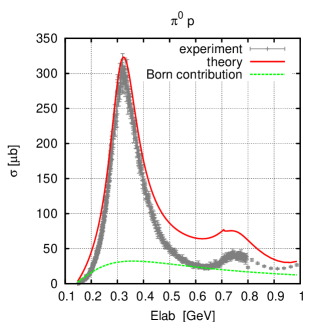
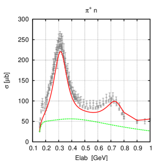
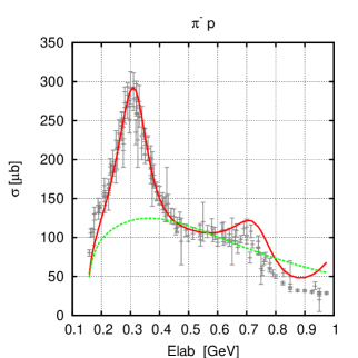
Figure 4: (Color online) Total cross section of pion photoproduction. Results of our calculation are compared with experimental data. Dashed lines show the contribution of Born diagrams.

V Results for dilepton production

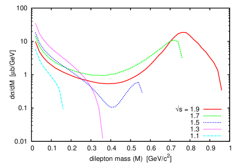
Figure 5: (Color online) Dilepton invariant mass spectra from the reaction $\pi^{-}+p\rightarrow n+e^{+}+e^{-}$ for various collision energies.

We used the effective field theory model described in Sec. III to calculate the matrix elements of the process $\pi^{-}+p\rightarrow n+e^{+}+e^{-}$ represented by the Feynman diagrams of Fig. 2. Then we used Eq. (6) to calculate the differential cross section $d\sigma/dM$. The integrations were carried out numerically using a Monte Carlo technique. The resulting dilepton spectra for various collision energies are shown in Fig. 5. The mass spectra at 1.3 GeV and below are monotonically decreasing, above 1.5 GeV pion energy the $\rho$ meson contributes. At 1.5 and 1.7 GeV energy only the tail of the $\rho$ meson spectrum is populated, still it produces a peak in the dilepton invariant mass spectrum. Note, however, that in the model no direct $\rho$ channel is included. The effect of the $\rho$ meson is encoded in the VMD form factors of hadrons.

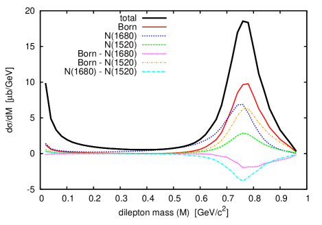
Figure 6: (Color online) Contributions of the dominant channels to the dilepton invariant mass spectrum of the reaction $\pi^{-}+p\rightarrow n+e^{+}+e^{-}$ at $\sqrt{s}=1.9$ GeV energy. See the text for the precise definition of the channels.

As the center-of-mass energy increases from 1.3 GeV to 1.9 GeV the importance of different resonances also changes. At 1.3 GeV the $s$-channel $\Delta(1232)$ contribution dominates the dilepton cross section. On the other hand at 1.9 GeV the Born term and the $s$-channel $N(1680)$ gives the dominant contribution. The $s$-channel $N(1520)$ diagram is also important. These can be seen in Fig. 6 which shows the contributions of the dominant channels to the dilepton spectrum at $\sqrt{s}=1.9$ GeV center-of-mass energy. Similarly to pion photoproduction, $u$-channel resonance contributions are always negligible after the inclusion of the cutoff Eq. (80).

In Fig. 6 we also show the contribution of the interference terms of the dominant channels. Note that interference terms can be negative, therefore we used a linear scale on the vertical axis. Since the interference terms are not negligible, dilepton production in $\pi N$ collisions cannot be approximated by the incoherent sum of $s$-channel baryon resonance diagrams Fig. 2(f), (which is the usual assumption in transport models), even if a background term is added to simulate the Born term. The simplest solution for transport models is to use the cross section calculated by the sum of all diagrams shown in Fig. 2. There is a price to pay for that: it is difficult to study in medium modification of baryon resonances in heavy ion reactions.

VI Conclusion

We have developed an effective field theoretical model to calculate the $\pi N\rightarrow Ne^{+}e^{-}$ cross section. We constructed an effective Lagrangian including nucleons, photons, pions and $\rho$ mesons (via VMD), and 16 baryon resonances below 2 GeV, i.e. all states with three- or four-star status except $\Delta(1950)$ and $\Delta(1920)$. We applied form factors at each vertex for internal hadron lines to account for their off-shell behavior. To maintain gauge invariance we generalized the method of Davidson-Workman Davidson-Workman to the production of massive photons (with and without an intermediate $\rho$ meson). The $NN\pi$ and $\pi\pi\rho$ couplings are well known. In the derivation of the interaction Lagrangians we used the electromagnetic gauge invariance and a model inspired by SU(2) gauge theory with $\rho$ mesons as gauge bosons. This model gives relations between some of the coupling constants.

Coupling constants of baryon resonances to the $N\pi$ and $N\rho$ channels have been determined from the appropriate partial width of the resonance, while the $RN\gamma$ couplings constants have been fitted to the pion photoproduction data.

For dilepton production we obtained monotonically decreasing invariant mass spectra below 1.5 GeV center-of-mass energy, while at higher energies the VMD form factor (related to the intermediate $\rho$ meson) creates a peak at high dilepton masses. The spectrum is dominated by the Born-term, but the $N(1680)$ and $N(1520)$ and their interference terms are sizable too. The importance of interference terms contradicts the usual assumption of transport models that the cross section is dominated by incoherent sum of $s$-channel resonance contributions.

References

• (1) W.K. Wilson et al. (DLS Collaboration), Phys. Rev. C 57, 1865 (1998).
• (2) G. Agakichiev et al. (HADES Collaboration), Phys. Lett. B 690, 118 (2010).
• (3) Gy. Wolf, G. Batko, W. Cassing, U. Mosel, K. Niita, and M. Schäfer, Nucl. Phys. A 517, 615 (1990).
• (4) E.L. Bratkovskaya, W. Cassing, M. Effenberger, and U. Mosel, Nucl. Phys. A 653, 301 (1999).
• (5) R. Shyam and U. Mosel, Phys. Rev. C 67, 065202 (2003).
• (6) L.P. Kaptari and B. Kämpfer, Nucl. Phys. A 764, 338 (2006).
• (7) L.P. Kaptari and B. Kämpfer, Eur. Phys. J. A 33, 157 (2007).
• (8) R. Shyam and U. Mosel, Phys. Rev. C 79, 035203 (2009).
• (9) L.P. Kaptari and B. Kämpfer, Phys. Rev. C 80, 064003 (2009).
• (10) R. Shyam and U. Mosel, Phys. Rev. C 82, 062201(R) (2010).
• (11) H. Garcilazo and E. Moya de Guerra, Nucl. Phys. A 562, 521 (1993).
• (12) T. Feuster and U. Mosel, Nucl. Phys. A 612, 375 (1997).
• (13) C. Fernández-Ramírez, E. Moya de Guerra, and J.M. Udías, Ann. Phys. (NY) 321, 1408 (2006).
• (14) J.J. Sakurai, Currents and mesons (University of Chicago Press, Chicago, 1969); Ann. Phys. (NY) 11, 1 (1960).
• (15) N.M. Kroll, T.D. Lee, and B. Zumino, Phys. Rev. 157, 1376 (1967).
• (16) H.B. O’Connell et al., Prog. Part. Nucl. Phys. 39, 201 (1997).
• (17) B. Friman and H.J. Pirner, Nucl. Phys. A 617, 496 (1997).
• (18) R.M. Davidson and R. Workman, Phys. Rev. C 63, 025210 (2001); 63, 058201 (2001).
• (19) L. Xiong, E. Shuryak, and G.E. Brown, Phys. Rev. D 46, 3798 (1992).
• (20) J.W. Durso and G.E. Brown, Nucl. Phys. A 430, 653 (1984).
• (21) J. Wess and B. Zumino, Phys. Rev. 163, 1727 (1976).
• (22) B.G. Yu, T.K. Choi, and W. Kim, Phys. Rev. C 83, 025208 (2011).
• (23) M. I. Krivoruchenko and B. V. Martemyanov, Annals of Physics 296, 299 (2002).
• (24) M. Zétényi and Gy. Wolf, Phys. Rev. C 67, 044002 (2003); Heavy Ion Phys. 17, 27 (2003).
• (25) S. Teis, W. Cassing, M. Effenberger, A. Hombach, U. Mosel and Gy. Wolf, Z. Phys. A 356, 421 (1997).
• (26) K. Nakamura et al. (Particle Data Group), J. Phys. G 37, 075021 (2010).