Can the nucleon axial charge be $O(N_{\rm c}^{0})$?

Abstract

The nucleon self-energy and its relation to the nucleon axial charge $g_{A}$ are discussed at large $N_{\rm c}$. The energy is compared for the hedgehog, conventional, and recently proposed dichotomous nucleon wavefunctions which give different values for $g_{A}$. We consider their energies at both perturbative and non-perturbative levels. In perturbative estimates, we take into account the pion exchanges among quarks up to the third orders of axial charge vertices, including the many-body forces such as the Wess-Zumino terms. It turns out that the perturbative pion exchanges among valence quarks give the same leading $N_{\rm c}$ contributions for three wavefunctions, while their mass differences are $O(\Lambda_{\rm QCD})$. The signs of splittings flip for different orders of the axial charge vertices, so it is hard to conclude which one is the most energetically favored. For non-perturbative estimates involving the modification of quark bases, we use the chiral quark soliton model as an illustration. With the hedgehog quark wavefunctions with $g_{A}$ of $O(N_{\rm c})$, we investigate whether solutions with coherent pions are energetically favored. Again it is hard to give decisive conclusions, but it is possible that adding the confining effects disfavors the solution with the coherent pions, making a pion cloud around a nucleon quantum rather than coherent. The nuclear matter at large $N_{\rm c}$ is also discussed in light of the value of $g_{A}$.

1 Introduction

Recently we discussed the phenomenological problems for nucleons at large $N_{\rm c}$, which are caused by the coherent pions surrounding nucleons [1]. The source of a coherent pion cloud is the large nucleon axial charge $g_{A}$ of $O(N_{\rm c})$, whose value depends upon quark wavefunctions inside a nucleon.

The problems related to large $g_{A}$ or coherent pions manifestly appear in the pion exchange part of the nuclear potential. Consider dilute nuclear matter where the pion exchange is the most important. For the nucleon-nucleon potential, the overall strength of the pion exchange is proportional to the square of the vertex, $(g_{A}/f_{\pi})^{2}\sim N_{\rm c}$. The kinetic energy of nucleons are at most $\sim\vec{p}^{2}/M_{N}\sim\Lambda_{\rm QCD}/N_{\rm c}$, so the kinetic energy is much smaller than the potential energy. It means that at large $N_{\rm c}$, nucleons localize at the potential minima, forming a crystal even at dilute regime [2, 3, 4, 5]. In reality, however, dilute nuclear matter is like a liquid where the potential and kinematic effects are equally important, and its binding energy is $O(1-10)$ MeV, hardly recognizable from the QCD scale $\Lambda_{\rm QCD}\sim 200$ MeV. For this qualitative discrepancy from the $N_{\rm c}=3$ world, usually the large $N_{\rm c}$ results are not regarded as useful guidelines for studies of a nuclear matter.

This situation, however, might be altered if the value of $g_{A}$ were not $O(N_{\rm c})$ but $O(1)$. With $g_{A}\sim 1$, both the potential and kinetic energy become comparable, $\sim\Lambda_{\rm QCD}/N_{\rm c}\sim 60$ MeV at $N_{\rm c}=3$, so it is much easier to expect the $O(1-10)$ MeV binding energy, by cancelling out the energetic cost and gain at the same order. Then the large binding energy problem could be solved, or at least be largely reduced. In this picture of small $g_{A}$, the long distance part of nucleon potentials should be described not by coherent pions but by a few quantum pions, and in fact, the latter has been a description in conventional nuclear physics [6, 7, 8]. Motivated by this observation, in Ref.[1] we started our attempt to construct the ground state nucleon wavefunction with $g_{A}\sim 1$ in case of the $SU(N_{\rm c})$ gauge theory. In this paper, we shall continue our discussions about a nucleon wavefunction with small $g_{A}$.

This reduction of $g_{A}$ itself does not solve all of the problems, however. We must handle a large attractive force of $O(N_{\rm c})$ at intermediate distance as well. It comes from the exchange of the $\sigma$-meson whose mass is supposed to be sensitive to $N_{\rm c}$ in contrast to other mesons [9, 10]. We imagine that at large $N_{\rm c}$, the range of $\sigma$ is comparable to the range of the strong repulsive force originating from the $\omega$ meson, and the spatial size of the attractive pocket becomes very small. Then the binding energies of nucleons would arise not from the leading $N_{\rm c}$ contributions, but from the $1/N_{\rm c}$ corrections. This aspect will be discussed elsewhere, but in what follows, the longest range part of the interaction must be first resolved before arguing the forces at intermediate distance. Therefore, as a first step, we focus on the pion problem.

The source of the axial charge $g_{A}$ is quark dynamics inside a nucleon. In this work, we will consider the valence quark contributions to the axial charge, $g_{A}^{{\rm val}}$, that is estimated from the valence nucleon wavefunction. As a theoretical guideline, in the following we consider problems in the context of the constituent quark picture, including the meson exchanges. If we include only the pions, the description we shall use is analogous to the frameworks of Manohar and Georgi [11], Weinberg [12], and Glozman and Riska [13]. Following a study of Weinberg [14], the quark axial charge is assumed to be $1$.

For considerations of the axial charge, it is convenient to use the $SU(4)$ spin-flavor generators [15, 16], formed by isospin, spin and axial charge operators:

$$\tau_{a}=\sum_{q}\tau_{a}^{(q)}\,,~{}\sigma_{i}=\sum_{q}\sigma_{i}^{(q)}\,,~{}R_{ai}=\sum_{q}R_{ia}^{(q)}=\sum_{q}\tau_{a}^{(q)}\sigma_{i}^{(q)}\,,$$ (1)

where $q$ means the operator acts on the $q$-th quark. Here we stress that we will not require the Hamiltonian and its eigenstates to be $SU(4)$ symmetric, and in fact, nucleons are not eigenstates of axial charge generators. The use of the $SU(4)$ generators is not mandatory step for our discussions. Nevertheless the use of the $SU(4)$ makes it easier to get several qualitative insights about quantities related to the axial charge operators. For instance, the diagonal axial charge of the proton with spin up is given by

$$g_{A}^{{\rm val}}=\langle p\!\uparrow\!|R_{33}|p\!\uparrow\rangle\,,$$ (2)

for the valence quark part. When we write $|p\!\uparrow\rangle$, it means the valence quark part for which we do not include extra contributions from induced pion clouds, etc., unless otherwise stated.

Below we will consider three types of the valence baryon wavefunctions in order. The hedgehog, conventional, and recently proposed dichotomous wavefunctions [1]. They provide different values of $g_{A}^{{\rm val}}$: $-N_{\rm c}$, $\pm(N_{\rm c}+2)/3$, and $\pm 1$, respectively.

In many studies, large $N_{\rm c}$ baryons are discussed starting with the baryon wavefunction of the hedgehog type [17]. The hedgehog state is a mixture of different spins and isospins but has a definite and very large axial charge, $g_{A}^{{\rm val}}=-N_{\rm c}$, that generates a large pion field. It allows us to apply the mean field or coherent picture of pions which is an underlying basis for the Skyrme type models [18, 19, 20], its holographic version [21, 22, 23], or chiral quark soliton models [24, 25, 26, 27, 28]. The states with definite isospin and spin can be obtained by collectively rotating the hedgehog wavefunction and the pion cloud. Therefore nucleons constructed in this way (we call them hedgehog nucleons) accompany a coherent pion cloud.

A more theoretically sound way to compute nucleon properties is to always keep the quantum numbers during calculations, although such computations are technically much more involved. It is nontrivial whether such a nucleon involves a coherent pion cloud or not. This is because once we fix the isospin and spin of a nucleon state, it is inevitably a mixture of different axial charge states (See discussions later).

In the conventional nucleon wavefunction, all quarks occupy the lowest $S$-wave orbit, and the spin-flavor wavefunction is maximally symmetrized to satisfy the Fermi statistics. The conventional nucleon wavefunction produces $g_{A}^{{\rm val}}=\pm(N_{\rm c}+2)/3$ at odd $N_{\rm c}$, while at even $N_{\rm c}$ it becomes zero [1] (here the “nucleon” at even $N_{\rm c}$ simply means the lowest isospin and spin state). This big sensitivity of $g_{A}^{{\rm val}}$ to whether $N_{\rm c}$ is odd or even is a consequence that a nucleon wavefunction is a superposition of different axial charge states. In particular, for an even $N_{\rm c}$ “nucleon”, the contributions from different axial charge states completely cancel out one another.

In the dichotomous wavefunction at odd $N_{\rm c}$, we place $N_{\rm c}-1$ quarks in the lowest $S$-wave orbit in such a way that they have zero isospin and spin. Then the remaining quark carries the same quantum number as nucleons, and we place it in a spatial orbit different from the other $N_{\rm c}-1$ quarks. As seen from the computation for the $N_{\rm c}$ even “nucleon”, the contributions to $g_{A}^{{\rm val}}$ from the $N_{\rm c}-1$ quarks cancel out one another, and $g_{A}^{{\rm val}}$ is saturated solely by a single quark. It means that $g_{A}^{{\rm val}}$ is $1$. An obvious question, however, is how to assure that the dichotomous state is energetically favored compared to the conventional one. To place one quark in an orbit different from the lowest $S$-wave orbit, we have to pay an energy penalty of $O(\Lambda_{\rm QCD})$.

Obviously which states appear as the ground state depends on the quark dynamics inside of the baryons. The purpose of this paper is to give the arguments on the energetic differences originating from the axial charge operators.

Our philosophy has several similarities with the chiral bag model as a hybrid model of quarks and pions [29, 30, 31]. Inside of a confining bag, there are quarks creating the axial charge as a source of pions. The strength of the source determines the size of the self-energy from the pion loops which modify the mass of the valence nucleon considerably. There are several versions depending on how we choose the size of the bag. But according to the Cheshire cat principle [32], it is just a matter of practice to make the computation of quarks and pions (with topological quark number) more tractable. Phrasing our treatment in this context, for the quark part we take a constituent quark model with the bag radius large enough to develop the constituent quark mass, and apply the non-relativistic framework to the computation of the valence axial charge.

We will argue the energy dependence of a nucleon on $g_{A}$ in perturbative and non-perturbative contexts. Unfortunately, it turns out that in both regimes, it is very hard to derive a definite conclusion about which one is the lightest state.

In a perturbative context, we consider pion exchanges among quarks inside a nucleon, which are supposed to be strongly correlated to the axial charge of a nucleon. The summation of their contributions depend on the spin-flavor wavefunctions, and are computed group theoretically. We evaluated the self-energy of baryons up to the terms quadratic and cubic in the axial charge operators. The Wess-Zumino vertices [33, 34, 35] are included. It turns out that the many-body forces or higher orders of axial charge operators appear at the same order of the leading $N_{\rm c}$, so that the convergence is not guaranteed.

We will argue that at the level of perturbative evaluations, the leading $N_{\rm c}$ contributions for hedgehog, conventional, and dichotomous wavefunctions are energetically degenerate. The pion exchange contributions for these wavefunctions differ by at most $O(\Lambda_{\rm QCD})$, at each order of the axial charge operators. So three wavefunctions differ in energy by $O(\Lambda_{\rm QCD})$ unless there are subtle cancellations among different orders of axial charge operators.

The computations based upon the perturbative pions are certainly insufficient, especially when we argue the nucleon with a large axial charge. When the strength of the pion field becomes very large, such a large pion field may drill a hole in a media of the chiral condensate, costing energy. Accordingly the constituent quark wavefunctions are modified as well. In this regime, we must take the non-perturbative effects into account at the stage determining the quark bases.

This kind of contribution is considered in the chiral quark soliton model including a full evaluation of the quark determinant [25, 26, 27, 28], provided that the background coherent pion field is of the hedgehog type. In this picture, the production of the coherent pion cloud costs energy of $O(N_{\rm c})$, while quarks acquire energetic gains of $O(N_{\rm c})$, by being bound to the pion cloud. The optimized configuration of pions and quarks is determined by the energetic balance between these $O(N_{\rm c})$ contributions.

We will see that for the hedgehog wavefunctions of quarks, it is justified to take the pion fields to be static and classical. Within a context of the chiral quark soliton picture, we give arguments why we expect that the hedgehog wavefunction is not energetically favored if the confining effects are included. The point is that the confining forces restrict the spatial size of quark wavefunctions, preventing deeply bound quarks to a pion cloud. On the other hand, for the conventional or dichotomous nucleon wavefunctions, we do not know how to take the appropriate mean field for pions, so we could not show the non-perturbative expressions of energies for these two wavefunctions.

In this paper, we discuss only two flavor cases, close to the chiral limit. Our metric is $g_{\mu\nu}={\rm diag}(1,-1,-1,-1)$.

This paper is organized as follows. Sec.2 is devoted to some preparation of basics which are used in later sections. We start with counting of the quark-meson coupling and classify its total contribution based on the spin-flavor wavefunctions of nucleons. Then we briefly review basic relations of the $SU(4)$ generators to the extent necessary for our arguments. In Sec.3, we show the construction of the hedgehog, conventional, and dichotomous wavefunctions, and compute their axial charges. In Sec.4, we compare the energies of three wavefunctions at the perturbative level. In Sec.5, we give non-perturbative considerations within a context of the chiral quark soliton picture. Sec.6 is devoted to summary.

2 Meson exchanges for the baryon self-energy: Preparations

In this section, we first argue how the meson exchanges among quarks contribute to the baryon mass. Especially we will focus on the meson exchange in the pion channel, because its quark-meson vertex has a form of the axial charge operator. For evaluations of the meson exchange contributions, it is useful to employ the $SU(4)$ spin-flavor algebra and its Casimir values at various orders. The many-body forces, including the Wess-Zumino vertex, will be discussed as well.

2.1 $N_{\rm c}$-counting

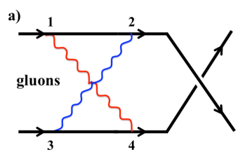
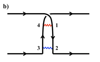
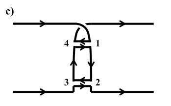
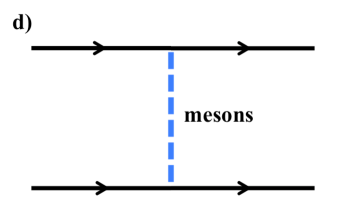
Figure 1: An example of two particle irreducible diagrams in which all gluon lines are crossed. We attached numbers to vertices to identify their locations after deforming quark lines. (a) Two gluon exchanges. (b) A deformed version of the diagram (a) which can be interpreted as a quark exchange. (c) A color line representation. There is a closed color line which provides an enhancement factor $N_{\rm c}$. (d) The corresponding meson exchange between quarks.

Suppose diagrams in which gluons are exchanged between two quarks. Diagrams that are obtained by iterations of a single gluon exchange may be treated within the one gluon exchange potential. On the other hand, there are also diagrams in which gluon exchange lines are all crossed, and are two particle irreducible (Fig.1). For the latter, by deforming quark lines it becomes manifest that the diagram is a planar one, and it is natural to interpret this quark exchange diagram as a meson exchange between two quarks.

Here one might think that at a distance scale among quarks inside of a baryon, it is not appropriate to consider quark exchanges as the meson exchanges. Such a terminology should not be taken too literally in this paper. The word “meson” is used as a representative of the two particle irreducible diagram such as Fig. 1(a), which carries the same quantum number as mesons. The person who dislikes this terminology can directly resum diagrams within the language of quarks and gluons. The real problem we cannot rigorously handle in this paper is rather the higher towers of mesons appearing at the distance scale $\sim\Lambda_{\rm QCD}^{-1}$, although it is likely that such mesons do not alter the main lines of our thoughts.

The meson exchanges among quarks can appear in the $O(N_{\rm c})$ contributions for the baryon self-energy, because there are many possible ways to choose the quark lines. We must keep them in the computation of the baryon mass as the leading order contributions. In the language of the effective Lagrangian for mesons and baryons, the meson exchanges among quarks correspond to the meson loops attached to a baryon line (Fig.2).

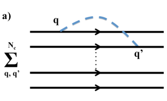
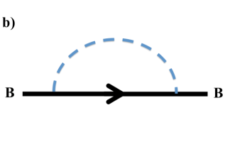
Figure 2: The self-energy diagram for a baryon. (a) The meson exchange among quarks. There are many possible ways to choose quark lines, $\sim N_{\rm c}^{2}$, whose contributions must be summed up. (b) The corresponding diagram in which a meson loop is attached to a baryon line.

As a reminder of the self-energy evaluation, consider diagrams such that one meson is exchanged between two quarks. Following the usual $N_{\rm c}$-counting, the intrinsic quark-meson coupling is given by $g_{qqM}\sim N_{\rm c}^{-1/2}$. One can choose two quark lines out of $N_{\rm c}$ quark lines, so its combinatorial factor is $\sim N_{\rm c}^{2}$. So if all of contributions are simply added without cancellations, one can estimate the contributions from these processes as $(g_{qqM})^{2}\times N_{\rm c}^{2}\sim N_{\rm c}$.

Actually, whether the total of the meson exchange contributions are large or not, strongly depends upon a spin-flavor wavefunction of a baryon.

The simplest example is the charge-charge interaction mediated by the $\omega_{0}$-meson exchange (the zeroth component of the $\omega$ meson). The $\omega_{0}$ couples to a quark number. Since all quarks have quark number $+1$, its sign always appears in the same sign. It means that all contributions are simply additive, so the self-energy is $(g_{qqM})^{2}\times N_{\rm c}^{2}\sim N_{\rm c}$.

There are many other examples in which various contributions cancel one another. Consider the $\rho_{0}$ exchanges which are responsible for the interactions among isospin charges. In contrast to the quark number, isospins of quarks may be either positive or negative, so that their contributions can cancel one another. For baryons with isospins of $O(1)$, the $\rho_{0}$-exchange diagrams happen to cancel out one another, producing negligible contributions, $g_{qqM}^{2}\times 1\sim 1/N_{\rm c}$. This process is important only for baryons with isospins of $O(N_{\rm c})$.

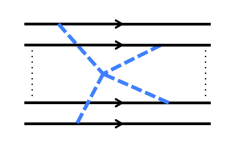
Figure 3: An example of the many-body forces in the baryon, induced by mesons. The diagram can appear at the leading $N_{\rm c}$ contribution.

In addition to the meson exchanges between two quarks, one must take into account many-body forces as well, because a quark density inside of a baryon is not dilute and there are many chances many mesons meet at once (Fig.3). Although the $n$-meson vertex behaves as $\sim N_{\rm c}^{1-n/2}$ and is suppressed, there are many ways to choose $n$-quark lines out of $N_{\rm c}$-quark lines, $\sim N_{\rm c}^{n}$. Each quark-meson vertex has $\sim N_{\rm c}^{-1/2}$, so as a total, the contributions from many-body forces can be $\sim N_{\rm c}^{1-n/2}\times N_{\rm c}^{n}\times N_{\rm c}^{-n/2}\sim N_{\rm c}$. In general, the tree diagrams of meson lines can appear at the leading order of $N_{\rm c}$.

This sort of arguments are also useful for the classification of the two-body and many-body forces in a baryonic matter. In fact, it has been used to interpret the hierarchy of the several meson exchange forces in the nucleon-nucleon potential [36].

2.2 The axial charge operator in the $SU(4)$ spin-flavor algebra

In this work, we will mainly focus on the diagrams involving pions, because we expect them most directly related to the axial charge of a baryon. Considering the non-linear realization of pions and quarks, their couplings contain at least one derivative. The lowest order coupling is given by

$$\mathcal{L}_{qq\pi}=g_{A}^{q}\,\frac{\partial^{\mu}\pi_{a}}{2f_{\pi}}\,\bar{q}\gamma_{\mu}\gamma_{5}\tau_{a}q\,.$$ (3)

We will take the quark axial charge $g_{A}^{q}$ to be $1$ [14].

We will take the non-relativistic approximation for quarks. This approximation is not rigorous for the quantitative estimates for the light quark system. But we expect that the relativistic corrections change overall strengths of the pion interactions equally for different wavefunctions, without affecting their energy ordering.

Applying the non-relativistic approximation for quarks in the baryons, the above vertex is simplified to

$$\langle B|\bar{q}\gamma_{\mu}\gamma_{5}\tau_{a}q(x)|B^{\prime}\rangle~{}\longrightarrow~{}\delta_{\mu i}\,\sum_{q}\langle B|\tau^{(q)}_{a}\sigma^{(q)}_{i}\delta(\vec{x}-\vec{r}^{(q)})|B^{\prime}\rangle\,\,,$$ (4)

where the zeroth component vanishes at the non-relativistic limit, and dominant contributions come from the spatial components. This matrix element carries the wavefunction dependence of the pion-baryon coupling. We shall evaluate it using the group theory.

The axial charge operators, together with isospin and spin operators, form the $SU(4)$ algebra. Writing operators

$$\tau_{a}=\sum_{q}\tau_{a}^{(q)}\,,~{}\sigma_{i}=\sum_{q}\sigma_{i}^{(q)}\,,~{}R_{ai}=\sum_{q}R_{ia}^{(q)}=\sum_{q}\tau_{a}^{(q)}\sigma_{i}^{(q)}\,,$$ (5)

their commutation relations are

$$[\,\tau_{a},\tau_{b}\,]=2\mathrm{i}\epsilon_{abc}\tau_{c}\,,~{}~{}~{}~{}[\,\sigma_{i},\sigma_{j}\,]=2\mathrm{i}\epsilon_{ijk}\sigma_{k}\,,$$

$$[\,\tau_{a},R_{bj}\,]=2\mathrm{i}\epsilon_{abc}R_{cj}\,,~{}~{}~{}~{}[\,\sigma_{i},R_{bj}\,]=2\mathrm{i}\epsilon_{ijk}R_{bk}\,,$$

$$[\,\tau_{a},\sigma_{j}\,]=0\,,~{}~{}~{}~{}[\,R_{ai},R_{bj}\,]=2\mathrm{i}\epsilon_{abc}\delta_{ij}\tau_{c}+2\mathrm{i}\epsilon_{ijk}\delta_{ab}\sigma_{k}\,.$$ (6)

Clearly, the operators $R_{ai}$ transform as vectors under the operations of isospin or spin rotations.

In the following, we classify the baryon states by specifying their eigenvalues of the Cartan bases for the $SU(4)$ algebra. As Cartan bases, we choose

$$(\,\tau_{3}\,,\sigma_{3}\,,R_{33}\,)\,,$$ (7)

where these operators commute one another so that we can label states with these quanta. The states in the irreducible representation $\mathcal{D}$ can be labeled as

$$|\tau_{3}\,,\sigma_{3}\,,R_{33}\,;\mathcal{D}\rangle\,.$$ (8)

For instance, fundamental representations are formed by single quarks

$$|u\!\uparrow\rangle=|1,1,1\rangle\,,~{}|d\!\uparrow\rangle=|-1,1,-1\rangle\,,~{}|u\!\downarrow\rangle=|1,-1,-1\rangle\,,~{}|d\!\downarrow\rangle=|-1,-1,1\rangle\,,~{}$$ (9)

which will be building blocks for the baryon wavefunctions. We will give their explicit forms in the next section.

2.3 The processes involving pions and their relations to the axial charge

Now let us see how these operators appear in the diagrams involving pions. We classify contributions by the order of the $R$ operators. For instance, one pion exchange between two quarks is the order of $R^{2}$, the diagram involving four pion emissions from four quarks and one $4\pi$ vertex is the order $R^{4}$, etc. Later we will evaluate the expectation values of these generators.

2.3.1 The $R^{2}$ operators: One pion exchange

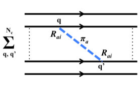
Figure 4: The one pion exchange contribution to the baryon mass. Its total size is proportional to the baryon matrix element for the $R_{ai}^{2}$ operator.

The simplest diagram contributing to the $R^{2}$ operator is the one pion exchange among quarks. We wish to evaluate the following matrix element (Fig.4)

$${\cal M}_{2\pi}=\langle B|\,\frac{\mathrm{i}^{2}}{4f_{\pi}^{2}}\!\int\mathrm{d}^{4}x\mathrm{d}^{4}y\,\big{(}\partial_{i}\pi_{a}(x)\,\bar{q}\gamma_{i}\gamma_{5}\tau_{a}q(x)\big{)}\,\big{(}\partial_{j}\pi_{b}(y)\,\bar{q}\gamma_{j}\gamma_{5}\tau_{b}q(y)\big{)}|B\rangle\,,$$ (10)

where we dropped off the zeroth component of the axial-vector current, taking the non-relativistic limit, Eq.(4). ${\cal M}_{2\pi}$ should be matched with the potential as ${\cal M}_{2\pi}=-\mathrm{i}\langle V_{2\pi}\rangle T$, because $\langle\mathrm{e}^{-\mathrm{i}(H_{0}+V)T}\rangle$.

We shall carry out the integration of virtual lines, leaving only quark operators. The pion propagator is

$$\big{\langle}T\,\partial_{i}\pi_{a}(x)\,\partial_{j}\pi_{b}(y)\big{\rangle}=\delta_{ab}\int\!\frac{\mathrm{d}^{4}p}{(2\pi)^{4}}\,\mathrm{e}^{-\mathrm{i}p(x-y)}\,\mathrm{i}\,\frac{\,p_{i}p_{j}\,}{\,p^{2}-m_{\pi}^{2}\,}\,.$$ (11)

In the non-relativistic limit, $p_{0}^{2}$ term in the denominator is smaller than the spatial component by $|\vec{p}|/M$ where $M$ is the constituent quark mass. Taking the non-relativistic limit, we decompose the propagator into the central and tensor parts,

$$\frac{\,p_{i}p_{j}\,}{\,p^{2}-m_{\pi}^{2}\,}\,\longrightarrow\,-\,\frac{\,\delta_{ij}\,}{3}\,\frac{\vec{p}^{2}}{\,\vec{p}^{2}+m_{\pi}^{2}\,}-\left(\frac{p_{i}p_{j}}{\vec{p}^{2}}-\frac{\,\delta_{ij}\,}{3}\right)\frac{\vec{p}^{2}}{\,\vec{p}^{2}+m_{\pi}^{2}\,}\,.$$ (12)

The second term is activated in the intermediate processes such that two quarks in the $S$-wave are scattered into the $D$-wave. We shall ignore such a contribution, and will take into account only the first term. Together with these simplifications,

$$\big{\langle}T\,\partial_{i}\pi_{a}(x)\,\partial_{j}\pi_{b}(y)\big{\rangle}\,\rightarrow\,-\,\frac{\mathrm{i}\delta_{ab}\delta_{ij}}{3}\,\delta(x_{0}-y_{0})\!\left(\delta^{3}(\vec{x}-\vec{y})-\frac{m_{\pi}^{2}}{4\pi}\frac{\,\mathrm{e}^{-m_{\pi}|\vec{x}-\vec{y}|}\,}{|\vec{x}-\vec{y}|}\right).$$ (13)

The reason why the $\delta$-function appears is that the derivative coupling of pions to quarks becomes larger for larger momentum transfer. It cancels out the $1/\vec{p}^{2}$ behavior of the pion propagator, so that the pion propagations with relatively high momenta are not suppressed (although in a more realistic treatment there should be the UV cutoff due to form factors). On the other hand, the second term is proportional to the pion mass, so disappears in the chiral limit.

In the chiral limit together with aforementioned approximations, Eq.(10) is reduced to

$${\rm Eq}.(\ref{onepi})\rightarrow\frac{\mathrm{i}}{12f_{\pi}^{2}}\int\mathrm{d}^{4}x\,\langle B|\bar{q}\gamma_{i}\gamma_{5}\tau_{a}q(x)\,\bar{q}\gamma_{i}\gamma_{5}\tau_{a}q(x)|B\rangle\,$$

$$=\frac{\mathrm{i}T}{12f_{\pi}^{2}}\int\mathrm{d}^{3}\vec{x}\,\sum_{q,q^{\prime}}\sum_{B^{\prime}}\,\langle B|R_{ai}^{(q)}\delta(\vec{x}-\vec{r}^{(q)})|B^{\prime}\rangle\langle B^{\prime}|R_{ai}^{(q^{\prime})}\delta(\vec{x}-\vec{r}^{(q^{\prime})})|B\rangle\,.$$ (14)

We mainly consider all quarks in $|B\rangle$ occupy the same spatial orbit, $\varphi$. To have nonzero matrix elements, quarks in $|B^{\prime}\rangle$ must occupy $\varphi$ except the $q$-th quark which hits the $\delta$-function. We ignore $|B^{\prime}\rangle$ including a radial excitation of a quark, and consider only $|B^{\prime}\rangle$ with all quarks in the spatial orbit $\varphi$. Then the equation is further simplified by summing the intermediate state $|B^{\prime}\rangle$,

$${\rm Eq}.(\ref{T2})\simeq\frac{\mathrm{i}T}{12f_{\pi}^{2}}\int\mathrm{d}^{3}\vec{x}\,\left|\varphi(\vec{x})\right|^{4}\,\langle B|R_{ai}^{2}|B\rangle_{{\rm SF}}\,.$$ (15)

where $|B\rangle_{{\rm SF}}$ means the spin-flavor part of $|B\rangle$. Therefore the potential is

$$\langle V_{2\pi}\rangle\simeq-\,\frac{1}{\,12f_{\pi}^{2}\,}\int\mathrm{d}^{3}\vec{x}\,\,|\varphi(\vec{x})|^{4}\,\langle B|R_{ai}^{2}|B\rangle_{{\rm SF}}\sim-\,\frac{\,\Lambda_{\rm QCD}^{3}\,}{12f_{\pi}^{2}}\,\langle B|R_{ai}^{2}|B\rangle_{{\rm SF}}\,,$$ (16)

which reduces the baryon mass. Here we assumed that the spatial extent of $\varphi(\vec{x})$ is $\sim\Lambda_{\rm QCD}^{-1}$, so that $|\varphi(\vec{x})|^{2}\sim\Lambda_{\rm QCD}^{3}$ from the normalization.

2.3.2 The $R^{3}$ operators: Wess-Zumino vertex

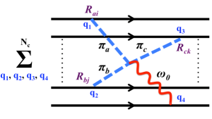
Figure 5: The $\omega$-$3\pi$ contribution to the baryon mass, mediated by the Wess-Zumino vertex. Its total size is proportional to the baryon matrix element for the $\epsilon_{abc}\epsilon_{ijk}R_{ai}R_{bj}R_{ck}$ operator.

Similar manipulations can be done also for higher order products of the $R$ operators. Here of particular interest is the $\omega$-$3\pi$ vertex coming from the Wess-Zumino term (Fig.5). The diagrams involving the $\omega$ meson are very important because $\omega_{0}$ strongly couples to a baryon due to its large quark number density of $O(N_{\rm c})$. In fact, in the Skyrme or chiral soliton models, this term is responsible for a repulsive force of $O(N_{\rm c})$ between a quark number density and a topological density, which stabilizes the configuration of the chiral soliton.

The quark-$\omega$ meson coupling appears in the form

$$\mathcal{L}_{\omega}=-g_{\omega}\omega_{\mu}\,\bar{q}\gamma^{\mu}q\,.$$ (17)

If we take the sign of $g_{\omega}$ in this way, the Wess-Zumino term for the $\omega-3\pi$ coupling is given by

$$\mathcal{L}_{\omega-3\pi}=\frac{N_{\rm c}g_{\omega}}{12\pi^{2}f_{\pi}^{3}}\,\epsilon^{\mu\nu\alpha\beta}\epsilon_{abc}\,\omega_{\mu}\,(\partial_{\nu}\pi_{a})\,(\partial_{\alpha}\pi_{b})\,(\partial_{\beta}\pi_{c})\,.$$ (19)

When evaluating this contribution for the baryon states, the term involving $\omega_{0}$ field is much larger than terms with $\omega_{i}$’s. Thus we consider only

$$\mathcal{L}_{\omega_{0}-3\pi}=-\frac{N_{\rm c}g_{\omega}}{12\pi^{2}f_{\pi}^{3}}\,\epsilon_{ijk}\epsilon_{abc}\,\omega_{0}\,(\partial_{i}\pi_{a})\,(\partial_{j}\pi_{b})\,(\partial_{k}\pi_{c})\,.$$ (20)

As before, we draw a diagram and integrate the virtual meson propagations, leaving the matrix element for quark operators. We compute

$${\cal M}_{\omega-3\pi} =\mathrm{i}^{5}\left(\frac{-1}{2f_{\pi}}\right)^{\!3}(-g_{\omega})\times\frac{-N_{\rm c}g_{\omega}}{12\pi^{2}f_{\pi}^{3}}\int\mathrm{d}^{4}x\,\mathrm{d}^{4}y\,\mathrm{d}^{4}z\,\mathrm{d}^{4}w\,\mathrm{d}^{4}u\,\langle B|\Gamma_{\omega-3\pi}|B\rangle$$

$$=-\mathrm{i}\,\frac{\,N_{\rm c}g_{\omega}^{2}\,}{96\pi^{2}f_{\pi}^{6}}\int\mathrm{d}^{4}x\,\mathrm{d}^{4}y\,\mathrm{d}^{4}z\,\mathrm{d}^{4}w\,\mathrm{d}^{4}u\,\langle B|\Gamma_{\omega-3\pi}|B\rangle\,,$$ (21)

where

$$\Gamma_{\omega-3\pi} =\big{(}\bar{q}\gamma_{i}\gamma_{5}\tau_{a}q(x)\big{)}\big{(}\bar{q}\gamma_{j}\gamma_{5}\tau_{b}q(y)\big{)}\big{(}\bar{q}\gamma_{k}\gamma_{5}\tau_{c}q(z)\big{)}\big{(}\bar{q}\gamma_{0}q(w)\big{)}$$

$$\times\big{(}\partial_{i}\pi_{a}(x)\big{)}\big{(}\partial_{j}\pi_{b}(y)\big{)}\big{(}\partial_{k}\pi_{c}(z)\big{)}\,\omega_{0}(w)$$

$$\times\epsilon_{lmn}\epsilon_{def}\,\omega_{0}(u)\,\big{(}\partial_{l}\pi_{d}(u)\big{)}\big{(}\partial_{m}\pi_{e}(u)\big{)}\big{(}\partial_{n}\pi_{f}(u)\big{)}\,.$$ (22)

The propagator of the $\omega$ meson, in the non-relativistic approximation, is

$$\big{\langle}T\omega_{0}(w)\,\omega_{\mu}(u)\big{\rangle} =\int\!\frac{\mathrm{d}^{4}p}{(2\pi)^{4}}\,\mathrm{e}^{-\mathrm{i}p(w-u)}\frac{-\mathrm{i}}{p^{2}-m_{\omega}^{2}}\left(g_{0\mu}-\frac{p_{0}p_{\mu}}{m_{\omega}^{2}}\right)$$

$$\simeq\mathrm{i}g_{0\mu}\,\delta(w_{0}-u_{0})\,G_{\omega}(\vec{w}-\vec{u})\,.$$ (23)

where

$$G_{\omega}(\vec{w}-\vec{u})=\frac{\mathrm{e}^{-m_{\omega}|\vec{w}-\vec{u}|}}{\,4\pi|\vec{w}-\vec{u}|\,}\,.$$ (24)

Assembling these approximations together, our vertex now takes the form

$${\cal M}_{\omega-3\pi}\rightarrow\mathrm{i}\,\frac{\,N_{\rm c}g_{\omega}^{2}T\,}{2^{4}3^{3}\pi^{2}f_{\pi}^{6}}\int\mathrm{d}\vec{x}\,\mathrm{d}\vec{w}\,\langle B|R^{(3)}(\vec{x})\,G_{\omega}(\vec{x}-\vec{w})\,Q_{0}(\vec{w})|B\rangle\,,$$ (25)

where we defined the cubic product of the axial charge operator,

$$R^{(3)}(\vec{x})\equiv\epsilon_{abc}\epsilon_{ijk}\,R_{ai}R_{bj}R_{ck}(\vec{x})\,,~{}~{}~{}R_{ai}(\vec{x})=\sum_{q}R_{ai}^{(q)}\delta(\vec{x}-\vec{r}^{(q)})\,,$$ (26)

and the quark number operator is $Q_{0}(\vec{w})=\bar{q}\gamma_{0}q(\vec{w})$. The quark number is very large, $N_{\rm c}$, for any baryon states. Again assuming that all quarks occupy the spatial orbit $\varphi$, then Eq.(25) becomes

$$\mathrm{i}\frac{\,N_{\rm c}g_{\omega}^{2}T\,}{\,2^{4}3^{3}\pi^{2}f_{\pi}^{6}\,}\,\langle B|R^{(3)}|B\rangle_{{\rm SF}}\int\mathrm{d}\vec{x}\,\mathrm{d}\vec{w}\,\,|\varphi(\vec{x})|^{6}\,G_{\omega}(\vec{x}-\vec{w})\times\left(N_{\rm c}\,|\varphi(\vec{w})|^{2}\right)\,.$$ (27)

This takes the form of the interaction between the distribution of the $R^{3}$ operator and the quark number density. Finally the potential energy is

$$\langle V_{\omega-3\pi}\rangle=-\frac{\,N_{\rm c}^{2}g_{\omega}^{2}\,}{\,2^{4}3^{3}\pi^{2}f_{\pi}^{6}\,}\,\langle B|R^{(3)}|B\rangle_{{\rm SF}}\int\mathrm{d}\vec{x}\,\mathrm{d}\vec{w}\,\,|\varphi(\vec{x})|^{6}\,G_{\omega}(\vec{x}-\vec{w})\,|\varphi(\vec{w})|^{2}\,.$$ (28)

As we will see, the $R^{3}$ term appears to be negative and $O(N_{\rm c}^{3})$. The overall factor is $N_{\rm c}^{2}g_{\omega}^{2}/f_{\pi}^{6}\sim 1/N_{\rm c}^{2}$, so $V_{\omega-3\pi}$ gives the energetic cost of $O(N_{\rm c})$.

3 Hedgehog, conventional, and dichotomous nucleon wavefunctions and their axial charges

In this section, we show explicit forms of the hedgehog, conventional, and dichotomous wavefunctions. Then we compute the expectation value of the $R_{33}$ operator.

3.1 A hedgehog nucleon wavefunction

The baryon wavefunction giving a hedgehog type configuration has zero grandspin, $\vec{G}\equiv\vec{\tau}+\vec{\sigma}=0$. The basic building block is a single quark wavefunction

$$\left(\frac{u\!\downarrow-d\!\uparrow}{\sqrt{2}}\right)\,,$$ (29)

which vanishes under the operation $\vec{G}\equiv\vec{\tau}+\vec{\sigma}$. (This choice is unique. Other wavefunction such as $\left(u\!\downarrow+d\!\uparrow\right)$ does not vanish under the operation of $\tau_{1}+\sigma_{1}$, etc.) The hedgehog baryon wavefunction is

$$|H\rangle=\left(\frac{u\!\downarrow-d\!\uparrow}{\sqrt{2}}\right)^{N_{\rm c}}\,.$$ (30)

This is just a product of the same single quark wavefunction, so it is maximally symmetric in spin-flavor. The special property is that $|H\rangle$ has a definite $R_{33}$ eigenvalue. Indeed, in the $SU(4)$ bases ($|\tau_{3},\sigma_{3},R_{33}\rangle$) one can write

$$\left(u\!\downarrow-d\!\uparrow\right)=|1,-1,-1\rangle-|-1,1,-1\rangle\,,$$ (31)

where the eigenvalue $R_{33}$ is common, so that its any products have a definite $R_{33}$ eigenvalue. But they are a linear superposition of the different $(\tau_{3},\sigma_{3})$. In these bases, the hedgehog wavefunction is written as

$$|H\rangle=\left(\frac{1}{\sqrt{2}}\right)^{\!N_{\rm c}}\sum_{n=0}^{N_{\rm c}}\,\sqrt{{}_{N_{\rm c}}C_{n}}\,(-1)^{n}\,|N_{\rm c}-2n,-(N_{\rm c}-2n),-N_{\rm c}\rangle_{{\rm MS}}\,,$$ (32)

where $|\cdots\rangle_{{\rm MS}}$ means that the state is maximally symmetrized. Here a factor $\sqrt{{}_{N_{\rm c}}C_{n}}$ is included to normalize the state as $\langle\tau_{3},\sigma_{3},R_{33}|\tau_{3},\sigma_{3},R_{33}\rangle_{\rm MS}=1$.

All the states contained in the hedgehog wavefunction have large $R_{33}$ eigenvalues of $O(N_{\rm c})$. So fluctuations of the $R_{33}$ charge, that are caused by the $SU(4)$ breaking terms in the Hamiltonian and happen in the time evolution, can be regarded as small fluctuations around the big mean value of $O(N_{\rm c})$. Thus the axial charge of the hedgehog state may be treated as classical and static mean field. We will use this observation when we give a non-perturbative consideration for the baryon self-energy.

The axial charge of the hedgehog state can be computed readily, and is given by $\langle H|R_{33}|H\rangle=-N_{\rm c}$, hence $g_{A}^{{\rm H}}=-N_{\rm c}$. The minimal eigenvalue $R_{33}$ for $N_{\rm c}$ quarks are $-N_{\rm c}$, so the hedgehog state saturates the lower bound of the baryon axial charge $g^{B}_{A}$.

3.2 A conventional nucleon wavefunction

The conventional nucleon wavefunctions have definite isospins and spins, while they are superpositions of different axial charge states. To construct states with small isospins and spins, it is convenient to prepare a $|I=0,S=0\rangle$ pair wavefunction as a building block:

$$|D\rangle =\frac{1}{2}\left|ud-du\right\rangle\otimes\left|\uparrow\downarrow-\downarrow\uparrow\right\rangle$$

$$=\frac{1}{2}\left|u\!\uparrow d\!\downarrow+\,d\!\downarrow u\!\uparrow\right\rangle-\frac{1}{2}\left|u\!\downarrow d\!\uparrow+\,d\!\uparrow u\!\downarrow\right\rangle$$

$$=\frac{1}{\sqrt{2}}\big{(}|0,0,2\rangle_{{\rm MS}}-|0,0,-2\rangle_{{\rm MS}}\big{)}\,,$$ (34)

which is a superposition of pair wavefunctions with different axial charge states, $R_{33}=\pm 2$.

Before going further, we stress that the construction of a nucleon from diquarks has nothing to do with any dynamical assumptions such as diquark correlations. In fact, at large $N_{\rm c}$ the diquark correlation is suppressed. Here we simply use the diquarks just for the convenience to prepare appropriate spin-flavor quantum numbers. Needless to say, we can arrive at the same wavefunction without using the diquark pair wavefunctions.

By just taking a direct product of these states, we can obtain spin-flavor functions with $I=S=0$. To construct $N_{\rm c}$ odd nucleons, we must further add one more quark to achieve the color singletness and appropriate spins. Then we totally symmetrize the spin-flavor-space wavefunctions for products of diquarks and an unpaired quark. Usually a nucleon with a maximally symmetric spin-flavor wavefunction are supposed to be the lowest energy state, because in this way one can place all of $N_{\rm c}$ quarks in the $S$-wave spatial orbit relative to the center of the nucleon.

Let us consider $|p^{{\rm c}}\!\uparrow\rangle$, conventional proton wavefunction, as an example. Its spin-flavor wavefunction is ($\mathcal{S}$ is the symmetrization operator)

$$|p^{{\rm c}}\!\uparrow\rangle_{{\rm SF}} =\mathcal{N}\mathcal{S}\big{[}|D\rangle^{n_{\rm d}}\otimes|u\!\uparrow\rangle\big{]}=\mathcal{N}\mathcal{S}\left[\big{(}\left|u\!\uparrow d\!\downarrow\right\rangle-\left|u\!\downarrow d\!\uparrow\right\rangle\big{)}^{n_{d}}\otimes|u\!\uparrow\rangle\right]$$

$$=\mathcal{N}\sum_{n=0}^{n_{d}}\,{}_{n_{d}}C_{n}\,(-1)^{n}\,\mathcal{S}\big{[}\,|u\!\uparrow\rangle^{n+1}\,|d\!\downarrow\rangle^{n}\,|u\!\downarrow\rangle^{n_{\rm d}-n}\,|d\!\uparrow\rangle^{n_{\rm d}-n}\,\big{]}\,,$$ (35)

where $N_{\rm c}=2n_{\rm d}+1$ and $\mathcal{N}$ is the normalization factor. For the $SU(4)$ bases, it is written as a superposition of states with different $R_{33}$ eigenvalues. Using the $R_{33}$ eigenvalues for $(u\!\uparrow,d\!\downarrow,u\!\downarrow,d\!\uparrow)=(1,1,-1,-1)$, we can write

$$|p^{{\rm c}}\!\uparrow\rangle_{{\rm SF}}=\mathcal{N}^{\prime}\sum_{n=0}^{n_{d}}\,{}_{n_{d}}C_{n}\,(-1)^{n}\,|\,1\,,1\,,4n+1-2n_{\rm d}\,\rangle_{{\rm MS}}\,.$$ (36)

This spin-flavor wavefunction contains states with both positive and negative $R_{33}$ eigenvalues. The mean value and fluctuations of the $R_{33}$ charge can be comparable during the time evolution. In addition, this makes the evaluation of $R_{33}$ expectation value for the conventional nucleon state much more nontrivial than for the hedgehog state. In fact, the contributions from states with positive and negative $R_{33}$ eigenvalues might strongly cancel one another. Our proposal of the dichotomous nucleon wavefunction, which will be discussed next, was motivated by this observation.

The axial charge of the conventional nucleon wavefunction has been computed in seminal works, and is given by

$$g_{A}^{{\rm c}}=\langle p^{{\rm c}}\!\uparrow\!|R_{33}|\,p^{{\rm c}}\!\uparrow\rangle_{{\rm SF}}=|\mathcal{N}^{\prime}|^{2}\sum_{n=0}^{n_{d}}\,\left({}_{n_{d}}C_{n}\right)^{2}\,(4n+1-2n_{\rm d})=\frac{\,N_{\rm c}+2\,}{3}\,,$$ (37)

where the contribution of $O(N_{\rm c})$ survives even after cancellations. Flipping either spin or isospin changes the sign of the axial charge, so $g_{A}^{{\rm c}}$ can be $\pm(N_{\rm c}+2)/3$ for nucleons.

3.3 A dichotomous nucleon wavefunction

The dichotomous wavefunction is constructed in such a way to make a nucleon axial charge $g_{A}$ small. To see how to achieve this, let us first consider the maximally symmetrized spin-flavor wavefunction made of $n_{\rm d}=(N_{\rm c}-1)/2$ diquarks with $I=S=0$,

$$\mathcal{S}\big{[}|D\rangle^{n_{\rm d}}\big{]}=\sum_{n=0}^{n_{d}}\,{}_{n_{d}}C_{n}\,(-1)^{n}\,|\,0\,,0\,,4n-2n_{\rm d}\,\rangle_{{\rm MS}}\,.$$ (38)

If we take the expectation value of $R_{33}$ for this state, we have

$$\mathcal{S}\big{[}\langle D|^{n_{\rm d}}\big{]}\,R_{33}\,\mathcal{S}\big{[}|D\rangle^{n_{\rm d}}\big{]}=\sum_{n=0}^{n_{d}}\,\left({}_{n_{d}}C_{n}\right)^{2}\,(4n-2n_{\rm d})=0\,,$$ (39)

where the contributions to the axial charge completely cancel out. From this, we can see that in the conventional nucleon, the $O(N_{\rm c})$ contribution arises from the overlap between the diquark part and an unpaired quark.

Therefore, if we place the unpaired quark in a spatial orbit different from other $(N_{\rm c}-1)/2$ quarks, the $O(N_{\rm c})$ contribution to the axial charge disappears. The dichotomous wavefunction for a proton with spin up is written as

$$|\,p^{{\rm d}}\!\uparrow\rangle=\mathcal{N}\,\mathcal{S}\big{[}|D;A\rangle^{n_{\rm d}}\otimes|u\!\uparrow;B\rangle\big{]}\,,$$ (40)

where the symmetrization is done for spin-flavor-space wavefunctions, by definition. Here $A$ and $B$ characterize spatial wavefunctions of quarks participating in the diquarks and an unpaired quark, respectively. When $A$ and $B$ are taken to be completely orthogonal, the axial charge is saturated by that of the unpaired quark,

$$g_{A}^{{\rm d}}=\langle\,p^{{\rm d}}\!\uparrow|\,R_{33}\,|\,p^{{\rm d}}\!\uparrow\rangle=\langle u\!\uparrow|\,R_{33}\,|\,u\!\uparrow\rangle=1\,.$$ (41)

So for the dichotomous nucleons, $g_{A}^{{\rm d}}=\pm 1$. The more general case where $A$ and $B$ are not completely orthogonal was computed in Ref.[1].

To avoid confusions, it is worth emphasizing that the dichotomous wavefunction is not an irreducible representation of the $SU(4)$ symmetry. We label quark bases with the eigenvalues of the $SU(4)$ generators, just for a matter of convenience to organize the computations of quantities related to the axial charge operators. Thus the use of the $SU(4)$ bases is not mandatory step. In fact, the states built from them need not be the irreducible representations of the $SU(4)$ symmetry because the Hamiltonian we are using is not $SU(4)$ symmetric. The point is that we are trying to distinguish different nucleon wavefunctions by the $SU(4)$ violating contributions. Whether the $SU(4)$ symmetry turns out to be good or not can be determined only after solving the dynamical problems.

The main problem when we try to regard the dichotomous state as the ground state is the kinetic energy cost when placing an unpaired quark in an orbit different from the others. Its energetic cost is $O(\Lambda_{\rm QCD})$. The self-energy contributions from pions must reduce the nucleon energy, compensating this energy cost.

4 Perturbative analyses

Now we have prepared all ingredients necessary for our perturbative considerations. In this section, we compare the nucleon mass for different wavefunctions, at the level of the perturbative contributions up to $O(R^{3})$ operators. It turns out that the hedgehog, conventional, and dichotomous wavefunctions give the same self-energy at the leading $N_{\rm c}$ contribution. At NLO of $N_{\rm c}$, the signs flip for different orders of the $R$-operators, so we cannot conclude which wavefunctions give the lowest energy at this level of analyses.

We will also argue specialities of the hedgehog state in these perturbative estimates, which will justifies the static mean field picture of the pion fields for the hedgehog quark wavefunction.

4.1 The contributions from the $R^{2}$ operator

To compute the one pion exchange contributions proportional to $R_{ai}^{2}$, we use the relation

$$R_{ai}^{2}=C_{2}-\tau_{a}^{2}-\sigma_{i}^{2}\,.$$ (42)

where $C_{2}$ is the second order Casimir. The largest contribution to $R_{ai}^{2}$ comes from $C_{2}$. For the maximally symmetric spin-flavor wavefunction of $n$ quarks, $C_{2}$ is given by

$$C_{2}\big{(}{\rm MS}(n)\big{)}=3n(n+4)\,,$$ (43)

(see Appendix. B.3). The hedgehog and conventional nucleon wavefunctions belong to the maximally symmetric spin-flavor representation of $N_{\rm c}$ quarks, and the expectation value of $C_{2}$ is given by $3N_{\rm c}(N_{\rm c}+4)$.

On the other hand, in the dichotomous wavefunction, $(N_{\rm c}-1)$ quarks and an unpaired quark have no overlap so that the expectation value of the Casimir is given by a sum of that of the $(N_{\rm c}-1)$ quarks and one unpaired quark. Then $C_{2}$ is given by $3(N_{\rm c}-1)(N_{\rm c}+3)+15=3N_{\rm c}^{2}+6N_{\rm c}+6$, which differs from other two wavefunctions by $O(N_{\rm c})$.

The expectation values of $\tau_{a}^{2}$ and $\sigma_{i}^{2}$ are trivial for the conventional and dichotomous wavefunctions with definite isospin and spin quantum numbers. The values are $\langle\tau_{a}^{2}\rangle=\langle\sigma_{i}^{2}\rangle=3$.

On the other hand, for the hedgehog state as a mixture of various isospin and spin states, we need a little manipulations. The hedgehog state contains isospins and spins of $O(N_{\rm c})$, so naively one might expect $O(N_{\rm c}^{2})$ contributions for $\langle\tau_{a}^{2}\rangle$ and $\langle\sigma_{i}^{2}\rangle$. It turns out, however, that $\langle\tau_{a}^{2}\rangle=\langle\sigma_{i}^{2}\rangle=3N_{\rm c}$ due to cancellations of $O(N_{\rm c}^{2})$ contributions (see Appendix. C.1).

Assembling all these results, the one pion exchange contribution is proportional to

$$-\,\langle R_{ai}^{2}\rangle=-3N_{\rm c}^{2}-6\times\left\{\begin{matrix}~{}N_{\rm c}~{}~{}~{}&({\rm hedgehog})\\ ~{}2N_{\rm c}-1~{}~{}~{}&~{}~{}~{}~{}({\rm conventional})\\ ~{}N_{\rm c}~{}~{}~{}&~{}~{}~{}~{}({\rm dichotomous})\end{matrix}\right.$$ (44)

after multiplying the overall sign for the potential energy. We do not find the difference at the leading order of $N_{\rm c}$. The conventional wavefunction acquires the largest attractive force at $O(R^{2})$. Since the intrinsic quark-meson coupling is $g_{\pi qq}\sim N_{\rm c}^{-1/2}$, the energy difference appears to be $\sim g_{\pi qq}^{2}\times N_{\rm c}\sim\Lambda_{\rm QCD}$.

Through Eq.(42), one can observe several interesting consequences for the excited states in the maximally symmetric representation. First, the single pion exchanges produce the same mass splitting rule for the higher isospin and spin multiplets. Second, for baryons with larger the isospins and/or spins, the self-energy contribution from the pion exchange is less important.

Finally we have to mention about the size of the $1/N_{\rm c}$ corrections. The expression $(\ref{R2Nc})$ explicitly contains the subleading terms of $1/N_{\rm c}$, and one can observe that the $1/N_{\rm c}$ corrections are substantial for $\langle R_{ai}^{2}\rangle$. We will return to this issue at Sec. 6.

4.2 The contributions from the $R^{3}$ operator

To compute the $R^{3}$-operators, we will use the relation,

$$\epsilon_{ijk}\epsilon_{abc}R_{ai}R_{bj}R_{ck}=-\,\frac{1}{\,4\,}\,C_{3}-8C_{2}+6R_{ai}\tau_{a}\sigma_{i}\,,$$ (45)

where $C_{3}$ is the third order Casimir. The relation directly follows by rewriting the expression of $C_{3}$ (see Appendix. B.4). As before, the largest contribution comes from $C_{3}$ which appears to be $O(N_{\rm c}^{3})$. For the maximally symmetric spin-flavor wavefunction of $n$ quarks, $C_{3}$ is

$$C_{3}\big{(}{\rm MS}(n)\big{)}=24\,n(n+4)(n-2)\,.$$ (46)

For the hedgehog and conventional wavefunctions, we substitute $n=N_{\rm c}$, and we get $\langle C_{3}\rangle=24N_{\rm c}(N_{\rm c}+4)(N_{\rm c}-2)$.

For the dichotomous wavefunction, we have a sum of $C_{3}$’s for $(N_{\rm c}-1)$-quarks and an unpaired quark. We get $24(N_{\rm c}-1)(N_{\rm c}+3)(N_{\rm c}-3)-120=24(N_{\rm c}^{3}-N_{\rm c}^{2}-9N_{\rm c}+4)$, which differs from other two wavefunctions by $O(N_{\rm c}^{2})$.

We already know the expectation values of $C_{2}$. The remaining $R\tau\sigma$ term yields

$$\langle R_{ai}\tau_{a}\sigma_{i}\rangle=\left\{\begin{matrix}-N_{\rm c}^{2}~{}~{}~{}&({\rm hedgehog})\\ ~{}3(N_{\rm c}+2)~{}~{}~{}&~{}~{}~{}~{}({\rm conventional})\\ ~{}9~{}~{}~{}&~{}~{}~{}~{}({\rm dichotomous})\end{matrix}\right.$$ (47)

The computation is given in Appendix.C.1. In particular, for the conventional and dichotomous wavefunctions, we will see $\langle R_{ai}\tau_{a}\sigma_{i}\rangle=9|\langle R_{33}\rangle|$.

Assembling all these results, the contribution from the $\omega-3\pi$ coupling is proportional to

$$-\epsilon_{abc}\epsilon_{ijk}\langle R_{ai}R_{bj}R_{ck}\rangle=6N_{\rm c}^{3}+6\times\left\{\begin{matrix}\,7N_{\rm c}^{2}+8N_{\rm c}~{}~{}&({\rm hedgehog})\\ \,6N_{\rm c}^{2}+5N_{\rm c}-6~{}~{}&~{}~{}~{}~{}({\rm conventional})\\ \,3N_{\rm c}^{2}-N_{\rm c}+3~{}~{}&~{}~{}~{}~{}({\rm dichotomous})\end{matrix}\right.$$ (48)

after multiplying the overall sign for the potential energy. The hedgehog state has the largest repulsive force. Again we do not find the difference at the leading order of $N_{\rm c}$. Considering the overall factors of the Wess-Zumino vertex and the quark number density of $O(N_{\rm c})$, the energy difference appears to be $\sim N_{\rm c}g_{\omega qq}^{2}/f_{\pi}^{6}\times N_{\rm c}\times N_{\rm c}^{2}\sim\Lambda_{\rm QCD}$.

Again we can explicitly see the size of $1/N_{\rm c}$ corrections. The $1/N_{\rm c}$ corrections are substantial as seen in $\langle R_{ai}^{2}\rangle$.

4.3 The hedgehog wavefunction and mean field pions

The hedgehog state has special properties in processes with perturbative pions. For linear $R$-operators, it has large axial charge distributions of $O(N_{\rm c})$,

$$\langle H|R_{33}|H\rangle=\langle H|R_{+-}|H\rangle=\langle H|R_{+-}|H\rangle=-N_{\rm c}\,,$$ (49)

or $\langle R_{11}\rangle=\langle R_{22}\rangle=\langle R_{33}\rangle=-N_{\rm c}$. All the other expectation values of the $R$ operators vanish.

Let us first see the $R^{2}$-operator. As we have seen, the sum of the axial charge operator is $\sim 3N_{\rm c}^{2}$. It means that the hedgehog state well-saturates the contributions from the intermediate states:

$$\sum_{a,i}\langle H|R_{ai}^{2}|H\rangle=\sum_{a,i}\sum_{n}\big{|}\langle H|R_{ai}|n\rangle\big{|}^{2}\,\geq\,\sum_{i=1}^{3}\big{|}\langle H|R_{ii}|H\rangle\big{|}^{2}=3N_{\rm c}^{2}\,,$$ (50)

where we used the hermiticity of $R_{ai}$.

The similar relation also holds for the $R^{3}$-operator. Its leading $N_{\rm c}$ contribution is $-6N_{\rm c}^{3}$, which can be obtained by saturating the intermediate state with the hedgehog state

$$\epsilon_{ijk}\epsilon_{abc}\langle H|R_{ai}R_{bj}R_{ck}|H\rangle=6\langle R_{11}\rangle_{H}\langle R_{22}\rangle_{H}\langle R_{33}\rangle_{H}+\cdots=-6N_{\rm c}^{3}+\cdots,$$ (51)

where $\cdots$ gives the remaining $O(N_{\rm c}^{2})$ contributions.

As we have just seen, for the hedgehog state, the distribution of the axial charge operators may be treated classically at large $N_{\rm c}$. Correspondingly, the mean field picture for pions is at work for the hedgehog state.

In contrast, usual baryon wavefunctions do not have this factorization property, and in fact, large contributions come from the transition amplitudes from one baryon to other baryon states. Thus quantum treatments are essential for these wavefunctions. In particular, for the dichotomous wavefunction, even if the expectation value of the linear operator $R$ (or the value of $g_{A}$) is small, the contributions from the off-diagonal matrix element are very large.

4.4 Color magnetic interaction

Here we shall consider one gluon exchange type processes and see how it affects the energy splitting among different wavefunctions.

The exchange of the spatial gluons (color-magnetic interaction) provides the spin splitting potential, ($\lambda=N_{\rm c}g_{s}^{2}$, and $\vec{r}_{qq^{\prime}}$ is distance between $q$-th and $q^{\prime}$-th quarks)

$$\sum_{q\neq q^{\prime}}V(\vec{r}_{qq^{\prime}})\sim\,\frac{\lambda}{N_{\rm c}}\sum_{q\neq q^{\prime}}\frac{~{}\sigma_{i}^{(q)}\sigma_{i}^{(q^{\prime})}}{M_{q}M_{q^{\prime}}}\,\delta(\vec{r}_{qq^{\prime}})\,,$$ (52)

which has been regarded as a source of the $N-\Delta$ splitting in the constituent quark models. Assuming all constituent quark masses are the same and computing the spatial part ($\psi(\vec{r}_{qq^{\prime}})$: relative spatial wavefunction), the matrix element can be written as

$$\left\langle\sum_{q\neq q^{\prime}}V(\vec{r}_{qq^{\prime}})\right\rangle \sim\,\frac{\,\lambda\,|\psi(\vec{0})|^{2}\,}{N_{\rm c}M^{2}}\,\left\langle\left(\sum_{q}\sigma_{i}^{(q)}\right)^{2}-\sum_{q}\left(\sigma_{i}^{(q)}\right)^{2}\right\rangle$$

$$=\frac{\,\lambda\,|\psi(\vec{0})|^{2}\,}{N_{\rm c}M^{2}}\,\left(\langle\sigma_{i}^{2}\rangle-3N_{\rm c}\right)\,.$$ (53)

The second term is common for different wavefunctions, so the difference comes from the first term. For conventional (or dichotomous) wavefunction with fixed spin of $S=1/2$, $\langle\sigma_{i}^{2}\rangle=3$, while for the hedgehog state, $\langle\sigma_{i}^{2}\rangle=3N_{\rm c}$. Since the interaction is repulsive, the color magnetic interaction lifts up the mass of the hedgehog state by $\sim\Lambda_{\rm QCD}$, compared to the conventional (or dichotomous) one. This is a consequence that the hedgehog state contains higher spin states.

5 Non-perturbative analyses: Chiral Quark Soliton

So far we have considered the perturbative contributions, provided that our wavefunctions have the same constituent quark bases with the same quark mass and quark-meson coupling. Then we found that different wavefunctions give the same baryon self-energy at the leading $N_{\rm c}$. However, once a large pion field is developed, the quark bases can be modified, and then the $O(N_{\rm c}^{0})$ modification for each quark mass may generate $O(N_{\rm c})$ difference for a baryon mass. We shall take into account such a possibility within the framework of the chiral quark soliton model.

As we discussed in the previous section, the static classical picture of the pion field should work for the hedgehog state, while it is difficult to apply this framework for the conventional and dichotomous wavefunctions. Therefore in this section, we consider the hedgehog wavefunction only, and discuss whether the generation of coherent pions is favored or not.

5.1 A baryon with the pion mean field

The chiral quark soliton model is a model which smoothly interpolates the constituent quark model and topological soliton model. We will work in the Euclidean space. We start with the following Lagrangian

$$\mathcal{L}=\bar{q}D(U_{5})q\,,~{}~{}~{}~{}\big{(}\,D(U_{5})=\left(\mathrm{i}{\ooalign{\hfil/\hfil\crcr$\partial$}}-MU_{5}\right)\,,~{}U_{5}=\exp\left[\mathrm{i}\gamma_{5}\tau_{a}\pi_{a}\right]\,\big{)}\,,$$ (54)

for which the regularized partition function is

$$Z=\int\mathcal{D}U\mathcal{D}q\mathcal{D}\bar{q}\,\mathrm{e}^{\,\mathrm{i}\int\mathrm{d}^{4}x\mathcal{L}}\,\big{|}_{{\rm reg.}}=\int\mathcal{D}U\exp\big{[}N_{\rm c}{\rm Tr}\,{\rm Ln}\left(D(U_{5})/D(U_{5}^{0})\right)\big{]}\,,$$ (55)

where $U=\exp(\mathrm{i}\tau_{a}\pi_{a})$. Here we divide the partition function with general $U_{5}$ by that with the vacuum configuration, $U_{5}^{0}=1$.

For the vacuum, the derivative expansion around $U_{5}^{0}=1$ generates the non-linear $\sigma$ model plus an infinite number of higher derivative terms, that are powers of $\partial U_{5}/M$, and the Wess-Zumino term [38]. The generation of the coherent pions should cost energy.

The single quark bases for a given pion background is obtained by solving the eigenvalue problem ($\tau=\mathrm{i}x^{0}$)

$$\gamma_{0}D(U_{5})\Phi_{n}=\big{(}\!-\partial_{\tau}-h(U_{5})\big{)}\Phi_{n}\,.~{}~{}~{}~{}\big{(}\,h(U_{5})=\gamma_{0}(\,\mathrm{i}\gamma_{k}\partial_{k}+MU_{5}\,)\,\big{)}$$ (56)

We will denote the single particle energy for general $U_{5}$ and $U_{5}^{0}$ as $\epsilon_{\alpha}$, $\epsilon_{\alpha}^{0}$, respectively. These bases are used for the evaluation of the quark determinant.

To compute the baryon spectra, we must consider the baryonic correlator at large time separation. It is given by

$$\langle J_{B}(\vec{0},T)\bar{J}_{B}(\vec{0},0)\rangle_{U_{5}} \sim\,\int\mathcal{D}U\exp\big{[}N_{\rm c}{\rm Tr}\,{\rm Ln}\left(D(U_{5})/D(U_{5}^{0})\right)\big{]}\,\prod_{i=1}^{N_{\rm c}}S_{q}(\vec{0},T;U_{5})$$

$$\sim\,\int\mathcal{D}U\exp\big{[}-T\,\big{(}E_{{\rm sea}}[U_{5}]+E_{{\rm val}}[U_{5}]\big{)}\big{]}\,,$$ (57)

where $E_{{\rm sea}}$ comes from the regularized Dirac determinant [25],

$$N_{\rm c}{\rm Tr}\,{\rm Ln}\left(D(U_{5})/D(U_{5}^{0})\right)=-TN_{\rm c}\sum_{\epsilon_{\alpha},\epsilon_{\alpha}^{0}<0}(\epsilon_{\alpha}-\epsilon_{\alpha}^{0})=-TE_{{\rm sea}}(U_{5})\,,$$ (58)

and is $O(N_{\rm c})$. This part is considered to be responsible for the polarization of the media that generates a pion cloud. Actually even after subtracting the trivial vacuum contribution, the sea contribution still diverges and has to be regularized by the UV cutoff. The coherent pion field affects quarks in the Dira sea with large negative energies.

On the other hand, the $E_{{\rm val}}$ is the valence quark contributions originating from the interpolating fields (the product of $N_{\rm c}$-propagators),

$$E_{{\rm val}}=\sum_{\alpha=1}^{N_{\rm c}}\epsilon^{\alpha}_{{\rm val}}(U_{5})\,,~{}~{}~{}(\epsilon_{{\rm val}}(U_{5}):{\rm the~{}level~{}above~{}the~{}Dirac~{}sea})$$ (59)

which is also $O(N_{\rm c})$. Here the $\epsilon_{{\rm val}}$ must appear above the Dirac sea because of the Pauli-blocking.

While the formal expression of the baryon mass is rather simple, its computation is quite tough. The derivative expansion around the vacuum configuration is hard to control, because the pion configuration varies at the scale of $\Lambda_{\rm QCD}^{-1}$. It means that all the higher powers of $\partial U_{5}/M$ equally contribute, so that it is necessary to completely diagonalize the quark determinant as well as the valence quark propagator. Such treatments have been carried out numerically in seminal works [25, 26, 27]. We will borrow their results for our discussions.

5.2 The optimized configuration within the stationary phase approximation

Note that the valence quark contributions are $O(N_{\rm c})$, thus can affect the optimal configuration of $U_{5}$ at large $N_{\rm c}$. The $U_{5}$ may deviate from $1$ at the classical level. We determine the optimal configuration $U_{5}$ from the following equation,

$$\delta_{U_{5}}\big{(}E_{{\rm sea}}[U_{5}]+E_{{\rm val}}[U_{5}]\big{)}\big{|}_{U_{5}=U_{5}^{c}}=0\,.$$ (60)

For two flavor case, we may parameterize $U_{5}$ as

$$U_{5}=\exp\big{[}\mathrm{i}\gamma_{5}\Theta(\vec{x})n_{a}(\vec{x})\tau_{a}\big{]}=\cos\Theta(\vec{x})+\mathrm{i}\gamma_{5}n_{a}(\vec{x})\tau_{a}\sin\Theta(\vec{x})\,,$$ (61)

where $n_{a}^{2}=1$. It is related to the linear realization as

$$\sigma(\vec{x})=M\cos\Theta(\vec{x})\,,~{}~{}~{}\pi_{a}(\vec{x})=n_{a}(\vec{x})M\sin\Theta(\vec{x})\,.$$ (62)

The $\Theta(\vec{x})$ is responsible for the fraction of the chiral density and pion density, while $n_{a}(\vec{x})$ characterizes orientations of pions in the isospin space.

In Eq.(60), if we take the variation with respect to $\Theta(\vec{x})$, it yields

$$\sin\Theta(\vec{x})\,\big{\langle}\bar{q}q(\vec{x})\big{\rangle}-n_{a}(\vec{x})\cos\Theta(\vec{x})\,\big{\langle}\bar{q}\mathrm{i}\gamma_{5}\tau_{a}q(\vec{x})\big{\rangle}=0\,.$$ (63)

Since the expectation value of the operators depend on the quark bases, this is the self-consistent equation.

5.3 The behaviors of $E_{{\rm field}}$ and $E_{{\rm val}}$

Consider first the trivial configuration $U_{5}=1\,(\Theta=0)$ for which $E_{{\rm sea}}=0$ by definition. Then the baryon mass is determined by the lowest quark energy orbit without a pion cloud, and $M_{B}=N_{\rm c}M$ at this level of the treatment. Thus if a nontrivial configuration of $U_{5}$ would exist, at least it must give smaller baryon mass than $N_{\rm c}M$.

Now suppose that the hedgehog quark wavefunction would give the ground state. Through the Dirac equation for the quark hedgehog wavefunctions [39], the form of $n_{a}(\vec{x})$ is fixed to $n_{a}(\vec{x})=r_{a}/r$, and $\Theta(\vec{x})=\Theta(r)$ where $\vec{r}=\vec{x}-\vec{x}_{0}$ ($\vec{x}_{0}$: the center of the baryon).

For this configuration, the boundary condition at $r\rightarrow 0$ is imposed to avoid the singularity related to the angular variable $n_{a}$ or $\pi_{a}$. It requires $\Theta(r)\rightarrow n\pi$ ($n$: integer) or $\pi_{a}(r)\rightarrow 0$ as $r\rightarrow 0$. The integer $n$ appears to correspond to the topological number of the meson profile. On the other hand $\Theta(r)\rightarrow 0$ as $r\rightarrow\infty$ to recover the vacuum configuration at asymptotic distance.

We have to solve the self-consistent equation (63) numerically. Instead, we use the profile function

$$\Theta(r;R)=-\pi\exp(-r/R)\,,$$ (64)

to see the general tendency of a single particle spectrum and the Dirac sea contributions in the presence of the hedgehog background. Actually, the self-consistent solution of Eq. (63) is known to give the similar form [26]. Here $R$ is treated as a variational parameter.

Clearly $E_{{\rm sea}}$ is a monotonously increasing function of $M$ or $R$. Meson profiles with larger $R$ and $M$ just increase the energy cost to make a hole in the vacuum condensate. On the other hand, the single particle energy $E_{{\rm val}}$ is a monotonously decreasing function of $M$ or $R$. The couplings between quark and mesons are attractive, so larger $M$ gives larger energy reduction. For larger $R$, the quark can be more deeply bound to the mesons, because of the smaller kinetic energy in the potential with broader range. At $MR\gg 1$, the valence energy level even enters the negative continuum, approaching to $-M$.

These tendencies are summarized in Fig.6 for our trial meson profile (64). The minimum (or local minimum) typically appear around $R\simeq(1-2)M^{-1}$ after cancelling out very large binding energy and sea quark contributions. The corresponding baryon is a mixture of valence quarks and coherent pions.

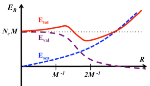
Figure 6: A schematic plot of $E_{{\rm val}}$, $E_{{\rm sea}}$, and their sum $E_{{\rm tot}}$ as a function of a meson cloud size $R$ in the profile (64). The decreasing behavior of $E_{{\rm val}}$ is due to a larger binding energy for a broader potential well. The increasing behavior of $E_{{\rm sea}}$ comes from the Dirac sea polarization. In $E_{{\rm tot}}$, the minimum is typically found at some value of $R$ between $M^{-1}$ and $2M^{-1}$, but the details about the height and locations of the minimum depend on the UV cutoff for the model. Here we took the UV cutoff to make the sea contribution small enough. With too large UV cutoff, the curve for $E_{{\rm sea}}$ is lifted up, making the minimum a local one.

Actually whether the minimum appears below or above depends on subtle details in calculations, such as the UV cutoff. The larger UV cutoff increases $E_{{\rm sea}}$ because in this model coherent pions even affect the energy level very deep in the Dirac sea, costing energy [26]. But in what follows, the existing literatures suggest that even if we find a nontrivial minimum with a coherent pion cloud, the energy reduction from $N_{\rm c}M$ is $20-30$% at most.

5.4 Spatial size of coherent pion and confining effects

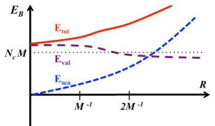
Figure 7: An expectation when the confining effects are included for the previous plot in Fig.6. (The confining potential lifts up the quark kinetic energy so even at $R\sim 0$, so the energy is higher than $N_{\rm c}M$.) The main modification appears in the behavior of $E_{{\rm val}}$. At distance scale $r\sim M^{-1}$, the linear potential closes a potential well made of a pion cloud, so the valence level does not acquire energy reduction much. As a consequence, the local minimum in $E_{{\rm tot}}$ would disappear.

The reduction of the baryon energy only comes from the quark binding to a pion cloud. The spatial size of the pion cloud must be so large, $R\geq M^{-1}$, that bound quark wavefunctions can spread out to avoid the kinetic energy cost.

However, the quark wavefunction cannot be widely spread out once confining effects are turned on. Our expectation is summarized in Fig.7. The confining force is activated when a quark is at distance of $r\sim\Lambda_{\rm QCD}^{-1}$ from the center of the baryon, giving the energetic cost of $\sim\sigma r\sim\Lambda_{\rm QCD}$. When we add contributions from the pion cloud potential and the linear potential, the potential well in the former with depth $\sim M$ is always closed at distance $r\sim M^{-1}$ by the linear potential, no matter how $R$ is large. Then the deeply bound valence quarks may not be allowed even at very large $R$.

As a consequence, it is possible that the nontrivial minimum, that was found within the chiral quark soliton model, disappears by including confining effects. As we have mentioned, the energy reduction by the quark binding to pions is not so large, so it is not surprising that confining effects lift the energy of the baryon with coherent pions above those without coherent pions. If this is indeed the case, the true energy minimum should be found at the small size of the coherent pion, $R\ll M^{-1}$. Then a number of pions becomes small, invalidating the mean field or coherent pion picture. We have to go back to the quantum calculations to treat quantum pions rather than coherent pions.

6 Summary

In this paper, we have discussed the energy differences among the hedgehog, conventional, and the dichotomous nucleon wavefunctions. Mainly we focus on the self-energy difference originating from the pion exchange which is related to the matrix element of the axial charge operators.

After examining both the perturbative and non-perturbative treatments of pions, we realize that it is very hard to derive decisive conclusions on the lowest energy state. The perturbative treatments give the same leading $N_{\rm c}$ behaviors for our three wavefunctions. In the non-perturbative treatments within the chiral quark soliton models, the existence of the state with coherent pions seems to be a subtle issue and depends upon details such as the UV cutoff and the confining force which are difficult to include in a solid way.

On the other hand, there seems to be a general tendency that both one gluon exchange and confining interaction generate extra energy costs for the hedgehog wavefunction, which is a representative state with coherent pions. Both effects are not manifest in typical chiral effective models. The combination of these effects with chiral models deserves further studies.

Clearly our analyses are incomplete. We dropped off exchanges of higher towers of mesons that couple to the axial charges. We expect that such resonances just change an overall size of the interactions, but do not alter the ordering of three wavefunctions. We have to check more carefully whether this expectation is correct or not, though.

Another oversimplification is the non-relativistic treatments. In particular, it is often said that at $N_{\rm c}=3$, the non-relativistic value of the axial charge is $5/3$ for the conventional nucleon, but it can be reduced to the experimental value $\simeq 1.26$ by including the down component of the Dirac spinor.

However, presumably this is not the end of the whole story. The nucleon $g_{A}$ was measured on the lattice for several pion masses [40, 41, 42]. The value is typically lower than the experimental value by about $10$%. What is nontrivial is that even at a large pion mass $\simeq 700$ MeV, $g_{A}$ remains small, $\simeq 1.1-1.2$. The non-relativistic treatments should work better for larger $m_{\pi}$ and higher constituent quark mass, reducing corrections from pion dynamics and relativistic effects. Thus we need explanations other than the relativistic corrections.

As for the lattice studies, it should be also mentioned that a lattice study of the baryon spectra is recently carried out for $N_{\rm c}=3,5,7$, in which the lowest pion mass is $(m_{\pi}/m_{\rho})^{2}\simeq 0.2$ (exp.: $\simeq 0.03$) [43]. The results show the rigid rotor spectra for the excited baryons, that are consistent with predictions from the color magnetic interaction, the perturbative pion exchange, and the collective excitations of the chiral soliton. The energy splitting is $\sim 1/N_{\rm c}$. Again we cannot judge which predictions are preferred, but we hope that eventually detailed studies of the pion mass dependence will distinguish these three contributions.

This lattice study also brought a serious constraint on the dichotomous wavefunction. Once we assumed the ground state with $I=S=1/2$ to be the small $g_{A}$ nucleon, it is natural to assume that the ground state with $I=S=3/2$ is the $\Delta$ baryon with small $g_{A}$. To construct such a $\Delta$ state, we need to bring two valence quarks into extra spatial orbits, costing energy of $\sim\Lambda_{\rm QCD}$ instead of $\sim\Lambda_{\rm QCD}/N_{\rm c}$ [1]. This contradicts with the lattice data for relatively large pion mass, while the dichotomous model is originally proposed to avoid a large pion cloud whose effects become substantial for small pion mass. The lattice studies for smaller pion mass may provide clear judgment for the validity of the dichotomous picture.

Finally we have to admit that the $1/N_{\rm c}$ corrections are substantial, at least in the perturbative estimates of the self-energy contributions (see the expressions, (44) and (48)). This fact may suggest us to revise our original proposal (see introduction), by taking a more appropriate leading order of the expansion.

Maybe a part of the problem comes from the fact that we put a large number of quarks into a small flavor space (two-flavor). It is interesting to check what happens if we take the Veneziano limit, $N_{\rm c},N_{\rm f}\rightarrow\infty$, $N_{\rm f}/N_{\rm c}=$ fixed. For instance, the second Casimir for the maximally symmetric representation is given by

$$C_{2}=(2N_{\rm f}-1)\times N_{\rm c}(N_{\rm c}+2N_{\rm f})\,.$$ (65)

It is clear that the $1/N_{\rm c}$ correction appears as the $N_{\rm f}/N_{\rm c}$ correction, and is substantial. Other quantities and their qualitative impacts on the nuclear physics will be discussed elsewhere.

Appendix A More on the $SU(4)$ algebra

For later calculations, we wish to write commutation relations in terms of the Cartan bases [45]. We choose the following Cartan generators $(H_{1},H_{2},H_{3})=(\tau_{3}\,,\sigma_{3}\,,R_{33})$. To find other bases, we must take appropriate linear combinations of $\tau$, $\sigma$, and $R$ to find generators $E_{\pm\alpha}$ such that

$$[\,H_{i}\,,E_{\pm\alpha}\,]=\pm\,\alpha_{i}E_{\pm\alpha}\,.$$ (66)

Let us find such linear combinations. First we define

$$\tau^{(q)}_{\pm}=\frac{\tau^{(q)}_{1}\pm\mathrm{i}\tau^{(q)}_{2}}{2}\,,~{}~{}~{}~{}\sigma^{(q)}_{\pm}=\frac{\sigma^{(q)}_{1}\pm\mathrm{i}\sigma^{(q)}_{2}}{2}\,,$$

$$R^{(q)}_{3\pm}=\tau^{(q)}_{3}\sigma^{(q)}_{\pm}\,,~{}~{}R^{(q)}_{\pm 3}=\tau^{(q)}_{\pm}\sigma^{(q)}_{3}\,,~{}~{}R^{(q)}_{\pm\pm}=\tau^{(q)}_{\pm}\sigma^{(q)}_{\pm}\,,~{}~{}R^{(q)}_{\pm\mp}=\tau^{(q)}_{\pm}\sigma^{(q)}_{\mp}\,.$$ (67)

Not all of these generators may be directly used as $E_{\pm\alpha}$. In particular, $\sigma_{\pm}$ and $\tau_{\pm}$ operators can not be used as raising and lowering operators for the irreducible representations of $SU(4)$, because states with definite $R_{33}$ eigenvalues are mixtures of states with different spins and isospins. It turns out that our bases are

$$E_{\pm\alpha^{(1)}}=R_{\pm 3}+\tau_{\pm}\,,~{}~{}~{}E_{\pm\alpha^{(2)}}=R_{\pm 3}-\tau_{\pm}\,,~{}~{}~{}E_{\pm\alpha^{(3)}}=R_{3\pm}+\sigma_{\pm}\,,$$

$$E_{\pm\alpha^{(4)}}=R_{3\pm}-\sigma_{\pm}\,,~{}~{}~{}E_{\pm\alpha^{(5)}}=2R_{\pm\pm}\,,~{}~{}~{}E_{\pm\alpha^{(6)}}=2R_{\pm\mp}\,.$$ (68)

Here the root vectors are

$$\vec{\alpha}^{(1)}=(2,0,2)\,,~{}~{}~{}\vec{\alpha}^{(2)}=(2,0,-2)\,,~{}~{}~{}\vec{\alpha}^{(3)}=(0,2,2)\,,$$

$$\vec{\alpha}^{(4)}=(0,2,-2)\,,~{}~{}~{}\vec{\alpha}^{(5)}=(2,2,0)\,,~{}~{}~{}\vec{\alpha}^{(6)}=(2,-2,0)\,,$$ (69)

which give the relation

$$[E_{\alpha^{(j)}},E_{-\alpha^{(j)}}]=\alpha_{i}^{(j)}H_{i}\,.$$ (70)

Appendix B The evaluation of Casimir operators

Here we briefly summarize the construction of the Casimir operators for the Lie algebra. To derive the general form, we follow the discussions of Okubo [44]. Then we use it to explicitly derive the formula for the maximally symmetric (MS) representations.

B.1 The general form

We consider generators of the Lie algebra

$$[X_{a},X_{b}]=f_{ab}^{~{}~{}c}X_{c}\,.$$ (71)

The general form of the Casimir operator is given by ($\tilde{C}_{p}$ can differ from $C_{p}$ by an overall factor which will be fixed later)

$$\tilde{C}_{p}=g^{a_{1}a_{2}\cdots a_{p}}X_{a_{1}}X_{a_{2}}\cdots X_{a_{p}}\,,$$ (72)

where $X_{a_{1}},\cdots,X_{a_{p}}$, are generators of the group, and

$$g_{\{\lambda_{0}\}}^{a_{1}a_{2}\cdots a_{p}}={\rm tr}_{\lambda_{0}}\left[X^{a_{1}}_{\{\lambda_{0}\}}X^{a_{2}}_{\{\lambda_{0}\}}\cdots X^{a_{p}}_{\{\lambda_{0}\}}\right]\,.$$ (73)

Here $X_{\{\lambda_{0}\}}$ means a generator in a representation $\{\lambda_{0}\}$ which we shall call a reference representation. For $\{\lambda_{0}\}$, we use the fundamental representation of $SU(2N_{\rm f})$ with ${\rm tr}_{{\rm fund.}}[1]=4$, and we raise and lower the indices using $g_{ab}=2N_{\rm f}\delta_{ab}$ and $g^{ab}=(g^{-1})_{ab}=\delta_{ab}/2N_{\rm f}$. We sometimes drop off the subscript $\{\lambda_{0}\}$ in $g^{a_{1}\cdots a_{p}}$ to simplify equations.

We wish to evaluate the value of the Casimir for any representations. Actually, once we compute the value of the quadratic Casimir for given representations, we can express the higher order Casimir using $C_{2}$’s. Below we briefly explain a main idea of the derivation.

Let us consider a product space $\{\lambda\}\otimes\{\lambda_{0}\}$, and its decomposition into irreducible representations,

$$\{\lambda\}\otimes\{\lambda_{0}\}=\sum_{j=1}^{N}\oplus\{\lambda_{j}\}\,.$$ (74)

In the RHS, there can be degeneracies of representations, for instance, it is possible that $\{\lambda_{k}\}=\{\lambda_{l}\}$ for $k\neq l$. We wish to compute the Casimir for the representation $\{\lambda\}$, using the fundamental representation for $\{\lambda_{0}\}$.

Consider a generator in the product space and its decomposition to irreducible representations,

$$X_{a}^{\{\lambda\otimes\lambda_{0}\}}=X_{a}^{\{\lambda\}}\otimes E^{\{\lambda_{0}\}}+E^{\{\lambda\}}\otimes X_{a}^{\{\lambda_{0}\}}=\sum_{j=1}^{N}X_{a}^{\{\lambda_{j}\}}P_{j}\,,$$ (75)

where $P_{j}$ is a projection operator picking out the $j$-th representation space. Clearly $\sum_{j}P_{j}=E^{\{\lambda\}}\otimes E^{\{\lambda_{0}\}}$.

Now let us define the following operator

$$Q_{\lambda;\lambda_{0}}\equiv X_{a}^{\{\lambda\}}\otimes X^{a}_{\{\lambda_{0}\}}=g^{ab}X_{a}^{\{\lambda\}}\otimes X_{b}^{\{\lambda_{0}\}}\,,$$ (76)

which commutes with all the generators in $\{\lambda\otimes\lambda_{0}\}$,

$$\left[Q_{\lambda;\lambda_{0}}\,,\,X_{a}^{\{\lambda\otimes\lambda_{0}\}}\right]=0\,.$$ (77)

Using this property, we can further show that the $p$-th order product

$$(Q_{\lambda;\lambda_{0}})^{p}=X_{a_{1}}^{\{\lambda\}}X_{a_{2}}^{\{\lambda\}}\cdots X_{a_{p}}^{\{\lambda\}}\otimes X^{a_{1}}_{\{\lambda_{0}\}}X^{a_{2}}_{\{\lambda_{0}\}}\cdots X^{a_{p}}_{\{\lambda_{0}\}}\,,$$ (78)

commutes with all the generators, and is the Casimir operator in the product space $\{\lambda\otimes\lambda_{0}\}$. Now taking the partial trace for $\{\lambda_{0}\}$, we obtain $g^{a_{1}\cdots a_{p}}$. Then the operator ${\rm tr}_{\lambda_{0}}[Q^{p}]$ gives the Casimir $\tilde{C}_{p}(\lambda)$ for the representation $\{\lambda\}$.

The relation between the $\tilde{C}_{p}(\lambda)$ and $\tilde{C}_{2}$’s follows from the property of the operator $Q_{\lambda;\lambda_{0}}$. We can rewrite $Q_{\lambda;\lambda_{0}}$ as a sum of $\tilde{C}_{2}$ for the representations $\{\lambda_{j}\}$, $\{\lambda\}$, and $\{\lambda_{0}\}$,

$$Q_{\lambda;\lambda_{0}} =g^{ab}\,X_{a}^{\{\lambda\}}\otimes X_{b}^{\{\lambda_{0}\}}$$

$$=\frac{g^{ab}}{2}\left[\left(X_{a}X_{b}\right)^{\{\lambda\otimes\lambda_{0}\}}-\left(X_{a}X_{b}\right)^{\{\lambda\}}\otimes E^{\{\lambda_{0}\}}-E^{\{\lambda\}}\otimes\left(X_{a}X_{b}\right)^{\{\lambda_{0}\}}\right]$$

$$=\frac{1}{2}\,\sum_{j=1}^{N}\big{[}\tilde{C}_{2}(\lambda_{j})-\tilde{C}_{2}(\lambda)-\tilde{C}_{2}(\lambda_{0})\big{]}P_{j}\,.$$ (79)

Below we will write $\xi_{\lambda_{j};\lambda,\lambda_{0}}=\big{[}\tilde{C}_{2}(\lambda_{j})-\tilde{C}_{2}(\lambda)-\tilde{C}_{2}(\lambda_{0})\big{]}/2$. Then the $p$-th order product is

$$(Q_{\lambda;\lambda_{0}})^{p}=X_{a_{1}}^{\{\lambda\}}\cdots X_{a_{p}}^{\{\lambda\}}\otimes X^{a_{1}}_{\{\lambda_{0}\}}\cdots X^{a_{p}}_{\{\lambda_{0}\}}=\sum_{j=1}^{N}\left(\xi_{\lambda_{j};\lambda,\lambda_{0}}\right)^{p}P_{j}\,.$$ (80)

Now a full trace of the operator $(Q_{\lambda;\lambda_{0}})^{p}$ for $\{\lambda\}$ and $\{\lambda_{0}\}$ gives the $p$-th order Casimir operator for $\{\lambda\}$ times the dimension of $\{\lambda\}$ (or the Casimir operator for $\{\lambda_{0}\}$ times the dimension of $\{\lambda_{0}\}$). The full trace in RHS gives a sum of the dimension for each representation $\{\lambda_{j}\}$. Therefore we finally find that

$$\tilde{C}_{p}(\lambda)=\sum_{j=1}^{N}\left(\xi_{\lambda_{j};\lambda,\lambda_{0}}\right)^{p}\,\frac{d(\lambda_{j})}{d(\lambda)}\,,$$ (81)

where $d(\lambda)$ is the dimension of the representation $\{\lambda\}$. To compute $\tilde{C}_{p}(\lambda)$, we need to know $\tilde{C}_{2}$’s of all the irreducible representations out of the product of $\{\lambda\}\otimes\{\lambda_{0}\}$.

B.2 The Casimirs for the maximally symmetric representations

In the following we will consider the Casimir for the MS representation for $n$-quarks. We need to compute the product of the MS($n$) representation and the fundamental representation which gives only two irreducible representations. In the Young tableaux,

$$\hskip 0.2pt\raisebox{0.0pt}{\makebox(6.5,6.5)[]{$$}}\raisebox{0.0pt}{\makebox(6.5,6.5)[]{$$}}\raisebox{0.0pt}{\makebox(6.5,6.5)[]{$$}}\raisebox{0.0pt}{\makebox(6.5,6.5)[]{$$}}\raisebox{0.0pt}{\makebox(6.5,6.5)[]{$$}}\hskip-0.2pt\hskip-32.5pt\raisebox{0.0pt}{\rule{32.5pt}{0.4pt}\hskip-32.5pt\rule{0.4pt}{6.5pt}\hskip 6.1pt\rule{0.4pt}{6.5pt}\hskip 6.1pt\rule{0.4pt}{6.5pt}\hskip 6.1pt\rule{0.4pt}{6.5pt}\hskip 6.1pt\rule{0.4pt}{6.5pt}\hskip 6.1pt\hskip-32.5pt\rule[6.5pt]{32.5pt}{0.4pt}\rule[6.5pt]{0.4pt}{0.4pt}\hskip-0.4pt\rule{0.4pt}{6.5pt}}\hskip-0.4pt\hskip-32.5pt\hskip 32.5pt\cdots\hskip 0.2pt\raisebox{0.0pt}{\makebox(6.5,6.5)[]{ $$}}\raisebox{0.0pt}{\makebox(6.5,6.5)[]{ $$}}\raisebox{0.0pt}{\makebox(6.5,6.5)[]{ $$}}\hskip-0.2pt\hskip-19.5pt\raisebox{0.0pt}{\rule{19.5pt}{0.4pt}\hskip-19.5pt\rule{0.4pt}{6.5pt}\hskip 6.1pt\rule{0.4pt}{6.5pt}\hskip 6.1pt\rule{0.4pt}{6.5pt}\hskip 6.1pt\hskip-19.5pt\rule[6.5pt]{19.5pt}{0.4pt}\rule[6.5pt]{0.4pt}{0.4pt}\hskip-0.4pt\rule{0.4pt}{6.5pt}}\hskip-0.4pt\hskip-19.5pt\hskip 19.5pt~{}~{}~{}\otimes~{}~{}\hskip 0.2pt\raisebox{0.0pt}{\makebox(6.5,6.5)[]{$$}}\hskip-0.2pt\hskip-6.5pt\raisebox{0.0pt}{\rule{6.5pt}{0.4pt}\hskip-6.5pt\rule{0.4pt}{6.5pt}\hskip 6.1pt\hskip-6.5pt\rule[6.5pt]{6.5pt}{0.4pt}\rule[6.5pt]{0.4pt}{0.4pt}\hskip-0.4pt\rule{0.4pt}{6.5pt}}\hskip-0.4pt\hskip-6.5pt\hskip 6.5pt~{}~{}=~{}~{}\hskip 0.2pt\raisebox{0.0pt}{\makebox(6.5,6.5)[]{$$}}\raisebox{0.0pt}{\makebox(6.5,6.5)[]{$$}}\raisebox{0.0pt}{\makebox(6.5,6.5)[]{$$}}\raisebox{0.0pt}{\makebox(6.5,6.5)[]{$$}}\raisebox{0.0pt}{\makebox(6.5,6.5)[]{$$}}\hskip-0.2pt\hskip-32.5pt\raisebox{0.0pt}{\rule{32.5pt}{0.4pt}\hskip-32.5pt\rule{0.4pt}{6.5pt}\hskip 6.1pt\rule{0.4pt}{6.5pt}\hskip 6.1pt\rule{0.4pt}{6.5pt}\hskip 6.1pt\rule{0.4pt}{6.5pt}\hskip 6.1pt\rule{0.4pt}{6.5pt}\hskip 6.1pt\hskip-32.5pt\rule[6.5pt]{32.5pt}{0.4pt}\rule[6.5pt]{0.4pt}{0.4pt}\hskip-0.4pt\rule{0.4pt}{6.5pt}}\hskip-0.4pt\hskip-32.5pt\hskip 32.5pt\cdots\hskip 0.2pt\raisebox{0.0pt}{\makebox(6.5,6.5)[]{ $$}}\raisebox{0.0pt}{\makebox(6.5,6.5)[]{ $$}}\raisebox{0.0pt}{\makebox(6.5,6.5)[]{ $$}}\raisebox{0.0pt}{\makebox(6.5,6.5)[]{ $$}}\hskip-0.2pt\hskip-26.0pt\raisebox{0.0pt}{\rule{26.0pt}{0.4pt}\hskip-26.0pt\rule{0.4pt}{6.5pt}\hskip 6.1pt\rule{0.4pt}{6.5pt}\hskip 6.1pt\rule{0.4pt}{6.5pt}\hskip 6.1pt\rule{0.4pt}{6.5pt}\hskip 6.1pt\hskip-26.0pt\rule[6.5pt]{26.0pt}{0.4pt}\rule[6.5pt]{0.4pt}{0.4pt}\hskip-0.4pt\rule{0.4pt}{6.5pt}}\hskip-0.4pt\hskip-26.0pt\hskip 26.0pt~{}~{}~{}\oplus~{}~{}\hskip 0.2pt\raisebox{0.0pt}{\makebox(6.5,6.5)[]{$$}}\raisebox{0.0pt}{\makebox(6.5,6.5)[]{$$}}\raisebox{0.0pt}{\makebox(6.5,6.5)[]{$$}}\raisebox{0.0pt}{\makebox(6.5,6.5)[]{$$}}\raisebox{0.0pt}{\makebox(6.5,6.5)[]{$$}}\hskip-0.2pt\hskip-32.5pt\raisebox{0.0pt}{\rule{32.5pt}{0.4pt}\hskip-32.5pt\rule{0.4pt}{6.5pt}\hskip 6.1pt\rule{0.4pt}{6.5pt}\hskip 6.1pt\rule{0.4pt}{6.5pt}\hskip 6.1pt\rule{0.4pt}{6.5pt}\hskip 6.1pt\rule{0.4pt}{6.5pt}\hskip 6.1pt\hskip-32.5pt\rule[6.5pt]{32.5pt}{0.4pt}\rule[6.5pt]{0.4pt}{0.4pt}\hskip-0.4pt\rule{0.4pt}{6.5pt}}\hskip-0.4pt\hskip-32.5pt\hskip 0.2pt\raisebox{-6.5pt}{\makebox(6.5,6.5)[]{$$}}\hskip-0.2pt\hskip-6.5pt\raisebox{-6.5pt}{\rule{6.5pt}{0.4pt}\hskip-6.5pt\rule{0.4pt}{6.5pt}\hskip 6.1pt\hskip-6.5pt\rule[6.5pt]{6.5pt}{0.4pt}\rule[6.5pt]{0.4pt}{0.4pt}\hskip-0.4pt\rule{0.4pt}{6.5pt}}\hskip-0.4pt\hskip-6.5pt\hskip 32.5pt\cdots\hskip 0.2pt\raisebox{0.0pt}{\makebox(6.5,6.5)[]{ $$}}\raisebox{0.0pt}{\makebox(6.5,6.5)[]{ $$}}\raisebox{0.0pt}{\makebox(6.5,6.5)[]{ $$}}\hskip-0.2pt\hskip-19.5pt\raisebox{0.0pt}{\rule{19.5pt}{0.4pt}\hskip-19.5pt\rule{0.4pt}{6.5pt}\hskip 6.1pt\rule{0.4pt}{6.5pt}\hskip 6.1pt\rule{0.4pt}{6.5pt}\hskip 6.1pt\hskip-19.5pt\rule[6.5pt]{19.5pt}{0.4pt}\rule[6.5pt]{0.4pt}{0.4pt}\hskip-0.4pt\rule{0.4pt}{6.5pt}}\hskip-0.4pt\hskip-19.5pt\hskip 19.5pt$$ (82)

In the RHS, the first one is the MS wavefunction of $(n+1)$-quarks, and the other is the mixed symmetric representation, which we will denote “mS”.

The dimension of the MS representation for $n$-quarks is given by

$$d\big{(}{\rm MS}(n)\big{)}=\frac{\,(n+2N_{\rm f}-1)!\,}{n!\,(2N_{\rm f}-1)!}\,.$$ (83)

By comparing both sides of the Young tableaux, we can find the dimension of the mS wavefunction with $(n+1)$-quarks as

$$d\big{(}{\rm mS}(n+1)\big{)} =d\big{(}{\rm MS}(n)\big{)}\times 2N_{\rm f}-d\big{(}{\rm MS}(n+1)\big{)}$$

$$=\frac{\,n\,(n+2N_{\rm f}-1)!\,}{(n+1)!\,(2N_{\rm f}-2)!}\,.$$ (84)

Since

$$\frac{d\big{(}{\rm MS}(n+1)\big{)}}{d\big{(}{\rm MS}(n)\big{)}}=\frac{\,n+2N_{\rm f}\,}{n+1}\,,~{}~{}~{}~{}~{}\frac{d\big{(}{\rm mS}(n+1)\big{)}}{d\big{(}{\rm MS}(n)\big{)}}=\frac{\,n\,(2N_{\rm f}-1)\,}{\,n+1\,}\,,$$ (85)

we find

$$\tilde{C}_{p}\big{(}{\rm MS}(n)\big{)}=\left(\xi_{{\rm MS}(n+1)}\right)^{p}\frac{\,n+2N_{\rm f}\,}{n+1}+\left(\xi_{{\rm mS}(n+1)}\right)^{p}\frac{\,n\,(2N_{\rm f}-1)\,}{\,n+1\,}\,.$$ (86)

The remaining task is the evaluation of the quadratic Casimir for the MS and mS representations.

B.3 The second order Casimir for MS and mS representations

The quadratic Casimir can be written in terms of the Cartan bases as follows:

$$C_{2}=\sum_{i=1}^{3}H_{i}^{2}+\sum_{j=1}^{6}\{E_{\alpha^{(j)}}\,,E_{-\alpha^{(j)}}\}\,.$$ (87)

This is related to $\tilde{C}_{2}=C_{2}/4$. ($\tilde{C}_{2}=X_{a}X^{a}=g^{ab}X_{a}X_{b}=\delta^{ab}X_{a}X_{b}/4$.) We will evaluate it for the MS and mS representations with $n$-quarks.

For the MS representation, we need to consider only the state with the highest weight, $(|u\!\uparrow\rangle)^{n}=|n,n,n\rangle$. In the second sum, $E_{\pm\alpha^{(j)}}|n,n,n\rangle=0$ for $j=2,4,6$, so only terms with $j=1,3,5$ can contribute for this state. Since $\vec{\alpha}^{(1)}=(2,0,2)$, $\vec{\alpha}^{(3)}=(0,2,2)$, and $\vec{\alpha}^{(5)}=(2,2,0)$, we have

$$C_{2}|n,n,n\rangle=\left(\sum_{i=1}^{3}H_{i}^{2}+4(\tau_{3}+\sigma_{3}+R_{33})\right)|n,n,n\rangle=3n(n+4)|n,n,n\rangle\,,$$ (88)

where we rewrite $\{E_{\alpha},E_{-\alpha}\}=[E_{\alpha},E_{-\alpha}]+2E_{-\alpha}E_{\alpha}$, and use the relation $[E_{\alpha^{(j)}},E_{-\alpha^{(j)}}]=\alpha_{i}^{(j)}H_{i}$.

Next we consider the mS wavefunction with $(n+1)$-quarks. First we prepare the highest weight wavefunction of the mS representation which is orthogonal to the MS wavefunction with the same $(\tau_{3},\sigma_{3},R_{33})$ values. Consider the MS wavefunction with the weight of the highest value minus one root,

$$|n-1,n-1,n+1\rangle_{{\rm MS}}\,\propto\,\mathcal{S}\,[\,|u\!\uparrow\rangle^{n}|d\!\downarrow\rangle]\,,$$ (89)

which can be rewritten as

$$\mathcal{S}\,\big{[}\,|u\!\uparrow\rangle^{n}|d\!\downarrow\rangle\big{]}=\mathcal{S}\,\big{[}\,|u\!\uparrow\rangle^{n}\big{]}\otimes|d\!\downarrow\rangle+n\,\mathcal{S}\,\big{[}\,|u\!\uparrow\rangle^{n-1}|d\!\downarrow\rangle\big{]}\otimes|u\!\uparrow\rangle$$

$$=n!\,\left(\,|n,n,n\rangle_{{\rm MS}}\otimes|d\!\downarrow\rangle+\sqrt{n}\,|n-2,n-2,n\rangle_{{\rm MS}}\otimes|u\!\uparrow\rangle\right)\,.$$ (90)

Then the mS wavefunction can be constructed as follows

$$|n-1,n-1,n+1\rangle_{{\rm mS}}$$

$$=\frac{1}{\sqrt{n+1\,}\,}\big{(}\sqrt{n}\,|n,n,n\rangle_{{\rm MS}}\otimes|d\!\downarrow\rangle-|n-2,n-2,n\rangle_{{\rm MS}}\otimes|u\!\uparrow\rangle\big{)}\,.$$ (91)

To evaluate the Casimir value, we decompose the generators as follows:

$$X_{a}^{2}=\left(\sum_{q=1}^{n}X_{a}^{(q)}+X_{a}^{(q^{\prime})}\right)^{2}=\left(\sum_{q=1}^{n}X_{a}^{(q)}\right)^{2}+2\sum_{q=1}^{n}X_{a}^{(q)}X_{a}^{(q^{\prime})}+(X_{a}^{(q^{\prime})})^{2}\,,$$ (92)

where the $X_{a}^{(q^{\prime})}$ acts on the $(n+1)$-th quark. The square operators give the Casimir values for the MS representation for $n$-quarks and a single quark. Nontrivial contributions come from the product of $n$-quark operators and a single quark operator, which can be rewritten as

$$\sum_{q=1}^{n}X_{a}^{(q)}X_{a}^{(q^{\prime})}=\sum_{q=1}^{n}\left(H_{i}^{(q)}H_{i}^{(q^{\prime})}+\sum_{j=1}^{6}\left(E_{\alpha^{(j)}}^{(q)}E_{-\alpha^{(j)}}^{(q^{\prime})}+E_{-\alpha^{(j)}}^{(q)}E_{\alpha^{(j)}}^{(q^{\prime})}\right)\right)\,.$$ (93)

When these product part act on the state $|n,n,n\rangle_{{\rm MS}}\otimes|d\!\downarrow\rangle$, only $H_{i}$ and $E_{\alpha^{(5)}}$ parts give the nonzero contributions. We find

$$\sum_{q=1}^{n}X_{a}^{(q)}X_{a}^{(q^{\prime})}|n,n,n\rangle_{{\rm MS}}\otimes|d\!\downarrow\rangle$$

$$=-n\,|n,n,n\rangle_{{\rm MS}}\otimes|d\!\downarrow\rangle+4\sqrt{n}\,|n-2,n-2,n\rangle_{{\rm MS}}\otimes|u\!\uparrow\rangle\,,$$ (94)

where we use the relation $\sum_{q}E^{(q)}_{-\alpha^{(5)}}|n,n,n\rangle=2\sqrt{n}\,|n-2,n-2,n\rangle$ and $E^{(q^{\prime})}_{\alpha^{(5)}}|d\!\downarrow\rangle=2\,|u\!\uparrow\rangle$. Similar calculations are applied to $|n-2,n-2,n\rangle_{{\rm MS}}\otimes|u\!\uparrow\rangle$, for which only $H_{i}$ and $E_{\alpha^{(5)}}$ survive. After summing these two contributions, one finds

$$\sum_{q=1}^{n}X_{a}^{(q)}X_{a}^{(q^{\prime})}|n-1,n-1,n+1\rangle_{{\rm mS}}=-(n+4)\,|n-1,n-1,n+1\rangle_{{\rm mS}}\,,$$ (95)

so that $C_{2}\big{(}{\rm mS}(n+1)\big{)}$ is given by

$$\left[\left(\sum_{q=1}^{n}X_{a}^{(q)}\right)^{2}+2\sum_{q=1}^{n}X_{a}^{(q)}X_{a}^{(q^{\prime})}+(X_{a}^{(q^{\prime})})^{2}\right]\,|n-1,n-1,n+1\rangle_{{\rm mS}}$$

$$=\big{[}\,C_{2}\big{(}{\rm MS}(n)\big{)}-2(n+4)+C_{2}\big{(}{\rm MS}(1)\big{)}\big{]}\,|n-1,n-1,n+1\rangle_{{\rm mS}}$$

$$=\left(3n+7\big{)}\big{(}n+1\right)\,|n-1,n-1,n+1\rangle_{{\rm mS}}\,.$$ (96)

In summary, the quadratic Casimir for the MS and mS representations are

$$C_{2}\big{(}{\rm MS}(n+1)\big{)} =3\,(n+5)(n+1)=4\,\tilde{C}_{2}\big{(}{\rm MS}(n+1)\big{)}\,,$$

$$C_{2}\big{(}{\rm mS}(n+1)\big{)} =(3n+7)(n+1)=4\,\tilde{C}_{2}\big{(}{\rm mS}(n+1)\big{)}\,,$$ (97)

so we have

$$\xi_{{\rm MS}(n+1)}=\frac{1}{\,2\,}\big{[}\,\tilde{C}_{2}\big{(}{\rm MS}(n+1)\big{)}-\tilde{C}_{2}\big{(}{\rm MS}(n)\big{)}-\tilde{C}_{2}(1)\,\big{]}=\frac{\,3n\,}{4}\,,$$

$$\xi_{{\rm mS}(n+1)}=\frac{1}{\,2\,}\big{[}\,\tilde{C}_{2}\big{(}{\rm mS}(n+1)\big{)}-\tilde{C}_{2}\big{(}{\rm MS}(n)\big{)}-\tilde{C}_{2}(1)\,\big{]}=-\,\frac{\,n+4\,}{4}\,.$$ (98)

Now we are ready to evaluate all the Casimirs for the MS($n$) representation.

B.4 The third order Casimir and its explicit form

Using $\xi_{{\rm MS}(n+1)}$ and $\xi_{{\rm mS}(n+1)}$, the cubic Casimir for the MS($n$) is

$$C_{3}\big{(}{\rm MS}(n)\big{)}=4^{3}\tilde{C}_{3}\big{(}{\rm MS}(n)\big{)} =4^{3}\left[\left(\xi_{{\rm MS}(n+1)}\right)^{3}\frac{\,n+4\,}{n+1}+\left(\xi_{{\rm mS}(n+1)}\right)^{3}\frac{\,3n\,}{\,n+1\,}\right]$$

$$=24\,n(n+4)(n-2)\,.$$ (99)

where we used $\tilde{C}_{3}=X_{a}X_{b}X_{c}{\rm tr}[X^{a}X^{b}X^{c}]=X_{a}X_{b}X_{c}{\rm tr}[X_{a}X_{b}X_{c}]/4^{3}=C_{3}/4^{3}$.

The contents of the cubic Casimir operator are the following. Apparently, there are $R^{3}$, $\tau^{3}$, $\sigma^{3}$, $R^{2}\tau$, $R^{2}\sigma$, $R\tau^{2}$, $R\sigma^{2}$, $R\tau\sigma$, $\tau^{2}\sigma$, $\tau\sigma^{2}$ terms, but nonzero traces come only from $R^{3}$, $\tau^{3}$, $\sigma^{3}$, $R^{2}\tau$, $R^{2}\sigma$, and $R\tau\sigma$ terms. We write

$$C_{3}=C(R^{3})+C(\tau^{3})+C(\sigma^{3})+C(R^{2}\tau)+C(R^{2}\sigma)+C(R\tau\sigma)\,.$$ (100)

$C(R^{3})$ is given by

$$C(R^{3})={\rm tr}\left[R_{ai}R_{bj}R_{ck}\right]R_{ai}R_{bj}R_{ck}=-4\,\epsilon_{abc}\epsilon_{ijk}R_{ai}R_{bj}R_{ck}\,.$$ (101)

$C(\tau^{3})$ is

$$C(\tau^{3})={\rm tr}\left[\tau_{a}\tau_{b}\tau_{c}\right]\tau_{a}\tau_{b}\tau_{c}=4\mathrm{i}\,\epsilon_{abc}\tau_{a}\tau_{b}\tau_{c}=-8\,\tau_{a}^{2}\,,$$ (102)

and $C(R^{2}\tau)$ is

$$C(R^{2}\tau) ={\rm tr}\left[R_{ai}R_{bj}\tau_{c}\right]R_{ai}R_{bj}\tau_{c}+{\rm tr}\left[R_{ai}\tau_{c}R_{bj}\right]R_{ai}\tau_{c}R_{bj}+{\rm tr}\left[\tau_{c}R_{ai}R_{bj}\right]\tau_{c}R_{ai}R_{bj}$$

$$=4\mathrm{i}\epsilon_{abc}\big{(}R_{ai}R_{bj}\tau_{c}-R_{ai}\tau_{c}R_{bj}+\tau_{c}R_{ai}R_{bj}\big{)}$$

$$=4\mathrm{i}\epsilon_{abc}R_{ai}[R_{bj},\tau_{c}]+2\mathrm{i}\epsilon_{abc}\tau_{c}[R_{ai},R_{bj}]$$

$$=-8\,\left(2R_{ai}^{2}+3\tau_{a}^{2}\right)\,.$$ (103)

We can obtain $C(\sigma^{3})$ and $C(R^{2}\sigma)$ terms as well. Finally $C(R\tau\sigma)$ term is

$$C(R\tau\sigma) ={\rm tr}\left[R_{ai}\tau_{b}\sigma_{j}\right]R_{ai}\tau_{b}\sigma_{j}+{\rm tr}\left[R_{ai}\sigma_{j}\tau_{b}\right]R_{ai}\sigma_{j}\tau_{b}+{\rm tr}\left[\tau_{b}R_{ai}\sigma_{j}\right]\tau_{b}R_{ai}\sigma_{j}$$

$$~{}~{}+{\rm tr}\left[\sigma_{j}R_{ai}\tau_{b}\right]\sigma_{j}R_{ai}\tau_{b}+{\rm tr}\left[\tau_{b}\sigma_{j}R_{ai}\right]\tau_{b}\sigma_{j}R_{ai}+{\rm tr}\left[\sigma_{j}\tau_{b}R_{ai}\right]\sigma_{j}\tau_{b}R_{ai}$$

$$=4\,\big{(}2R_{ai}\tau_{a}\sigma_{i}+2\tau_{a}\sigma_{i}R_{ai}+\tau_{a}R_{ai}\sigma_{i}+\sigma_{i}R_{ai}\tau_{a}\big{)}$$

$$=24R_{ai}\tau_{a}\sigma_{i}\,,$$ (104)

where we used $[R_{ai},\tau_{a}]=[R_{ai},\sigma_{i}]=0$ in the last line to change the ordering. Assembling all these terms, we have

$$C_{3}=-4\,\epsilon_{abc}\epsilon_{ijk}R_{ai}R_{bj}R_{ck}-32C_{2}+24R_{ai}\tau_{a}\sigma_{i}\,.$$ (105)

Appendix C Computations of various matrix elements

C.1 $\tau_{a}^{2}$ and $\sigma_{i}^{2}$ for the hedgehog state

We compute $\tau_{a}^{2}$ and $\sigma_{i}^{2}$ for the hedgehog wavefunction. For the third component of the isospin, we have

$$\langle H|\tau_{3}^{2}|H\rangle=\frac{1}{\,2^{N_{\rm c}}\,}\sum_{n=0}^{N_{\rm c}}{}_{N_{\rm c}}C_{n}\,(N_{\rm c}-2n)^{2}=N_{\rm c}\,.$$ (106)

For the other isospin operators, we have

$$\langle H|\left(\tau_{1}^{2}+\tau_{2}^{2}\right)|H\rangle =\frac{1}{2}\,\langle H|\left\{E_{\alpha^{(1)}}-E_{\alpha^{(2)}}\,,E_{-\alpha^{(1)}}-E_{-\alpha^{(2)}}\right\}|H\rangle$$

$$=\frac{1}{2}\,\langle H|\left(E_{-\alpha^{(1)}}E_{\alpha^{(1)}}+E_{\alpha^{(2)}}E_{-\alpha^{(2)}}\right)|H\rangle\,,$$ (107)

where we used the fact that $E_{-\alpha^{(1)}}|H\rangle=E_{\alpha^{(2)}}|H\rangle=\langle H|E_{-\alpha^{(2)}}=\langle H|E_{\alpha^{(1)}}=0$. (This is because $\vec{\alpha}^{(1)}=(2,0,2)$, $\vec{\alpha}^{(2)}=(2,0,-2)$, and the hedgehog state has the minimum of the axial charge, $R_{33}=-N_{\rm c}$.) Let us further note that

$$\langle H|\left(E_{-\alpha^{(1)}}E_{\alpha^{(1)}}+E_{\alpha^{(2)}}E_{-\alpha^{(2)}}\right)|H\rangle$$

$$= \,\langle H|\left([E_{-\alpha^{(1)}},E_{\alpha^{(1)}}]+[E_{\alpha^{(2)}},E_{-\alpha^{(2)}}]\right)|H\rangle=\langle H|(\vec{\alpha}^{(2)}-\vec{\alpha}^{(1)})_{i}H_{i}|H\rangle$$

$$= \,-4\,\langle H|R_{33}|H\rangle=4N_{\rm c}\,.$$ (108)

Applying the same manipulation to the spin operators, the hedgehog state has the following expectation values,

$$\langle H|\,\tau_{a}^{2}|H\rangle=3N_{\rm c}\,,~{}~{}~{}~{}~{}\langle H|\,\sigma_{i}^{2}|H\rangle=3N_{\rm c}\,.$$ (109)

C.2 The expectation value of the $R\tau\sigma$ operator

Next we compute $R_{ai}\tau_{a}\sigma_{i}$ in $C_{3}$ for various wavefunctions. First we write it as

$$R_{ai}\tau_{a}\sigma_{i} =R_{33}\tau_{3}\sigma_{3}+2\left(R_{+3}\tau_{-}\sigma_{3}+R_{-3}\tau_{+}\sigma_{3}+R_{3+}\tau_{3}\sigma_{-}+R_{3-}\tau_{3}\sigma_{+}\right)$$

$$~{}~{}+4\left(R_{++}\tau_{-}\sigma_{-}+R_{-+}\tau_{+}\sigma_{-}+R_{+-}\tau_{-}\sigma_{+}+R_{--}\tau_{+}\sigma_{+}\right)\,.$$ (110)

We first consider the conventional and dichotomous wavefunctions for the state $|p\!\uparrow\rangle$. The isospin and spin parts can be computed readily, and we have

$$\langle p\!\uparrow\!|R_{ai}\tau_{a}\sigma_{i}|p\!\uparrow\rangle=9\,\langle p\!\uparrow\!|R_{33}|p\!\uparrow\rangle\,,$$ (111)

where we used $\langle p\!\uparrow\!|R_{++}|n\!\downarrow\rangle=\langle p\!\uparrow\!|R_{+3}|n\!\uparrow\rangle=\langle p\!\uparrow\!|R_{3+}|p\!\downarrow\rangle=\langle p\!\uparrow\!|R_{33}|p\!\uparrow\rangle$, and $\tau_{-}|p\!\uparrow\rangle=|n\!\uparrow\rangle$, etc.

For the hedgehog wavefunction, it is useful to note that $(\tau_{a}^{(q)}+\sigma_{i}^{(q)})|H\rangle=0$ for each $q$. Then, for instance,

$$\langle H|R_{33}\tau_{3}\sigma_{3}|H\rangle=-N_{\rm c}\langle H|\tau_{3}\sigma_{3}|H\rangle=N_{\rm c}\langle H|\tau_{3}^{2}|H\rangle=N_{\rm c}^{2}\,,$$ (112)

or another example is

$$\langle H|R_{++}\tau_{-}\sigma_{-}|H\rangle=-\sum_{q}\langle H|(\tau_{+}^{(q)})^{2}\tau_{-}\sigma_{-}|H\rangle=0\,,$$ (113)

since $\tau_{+}^{(q)}$ is the fundamental representation. Doing similar manipulations, finally we arrive at

$$\langle H|R_{ai}\tau_{a}\sigma_{i}|H\rangle=-N_{\rm c}^{2}\,.$$ (114)

References

- [1] Y. Hidaka, T. Kojo, L. McLerran and R. D. Pisarski, Nucl. Phys. A 852 (2011) 155 [arXiv:1004.2261 [hep-ph]].
- [2] M. Kutschera, C. J. Pethick and D. G. Ravenhall, Phys. Rev. Lett. 53 (1984) 1041.
- [3] I. R. Klebanov, Nucl. Phys. B 262 (1985) 133.
- [4] M. Kugler and S. Shtrikman, Phys. Rev. D 40 (1989) 3421; M. Kugler and S. Shtrikman, Phys. Lett. B 208 (1988) 491; L. Castillejo, P. S. J. Jones, A. D. Jackson, J. J. M. Verbaarschot and A. Jackson, Nucl. Phys. A 501 (1989) 801; T. S. Walhout, Nucl. Phys. A 484 (1988) 397; E. Braaten, S. Townsend and L. Carson, Phys. Lett. B 235 (1990) 147. N. S. Manton, Commun. Math. Phys. 111 (1987) 469.
- [5] K. Nawa, H. Suganuma and T. Kojo, Phys. Rev. D 79 (2009) 026005 [arXiv:0810.1005 [hep-th]]; M. Rho, S. -J. Sin and I. Zahed, Phys. Lett. B 689 (2010) 23 [arXiv:0910.3774 [hep-th]].
- [6] H. Yukawa, Proc. Phys. Math. Soc. Jap. 17 (1935) 48; M. Taketani, S. Nakamura and M. Sasaki, Prog. Theor. Phys. 6 (1951) 581; M. Taketani, S. Machida and S. O-numa Prog. Theor. Phys. 7 (1952) 45.
- [7] M. Lacombe, B. Loiseau, J. M. Richard, R. Vinh Mau, J. Cote, P. Pires and R. De Tourreil, Phys. Rev. C 21 (1980) 861; R. Machleidt, K. Holinde and C. Elster, Phys. Rept. 149 (1987) 1; R. B. Wiringa, V. G. J. Stoks and R. Schiavilla, Phys. Rev. C 51 (1995) 38 [nucl-th/9408016]; V. G. J. Stoks, R. A. M. Klomp, C. P. F. Terheggen and J. J. de Swart, Phys. Rev. C 49 (1994) 2950 [nucl-th/9406039].
- [8] For review, R. Machleidt, Adv. Nucl. Phys. 19 (1989) 189.
- [9] J. R. Pelaez, Phys. Rev. Lett. 92 (2004) 102001 [hep-ph/0309292]; J. R. Pelaez and G. Rios, Phys. Rev. Lett. 97 (2006) 242002 [hep-ph/0610397]; C. Hanhart, J. R. Pelaez and G. Rios, Phys. Rev. Lett. 100 (2008) 152001 [arXiv:0801.2871 [hep-ph]]; J. Ruiz de Elvira, J. R. Pelaez, M. R. Pennington and D. J. Wilson, Phys. Rev. D 84 (2011) 096006 [arXiv:1009.6204 [hep-ph]].
- [10] T. Kojo and D. Jido, arXiv:0807.2364 [hep-ph]; ibid. Phys. Rev. D 78 (2008) 114005 [arXiv:0802.2372 [hep-ph]].
- [11] A. Manohar and H. Georgi, Nucl. Phys. B 234 (1984) 189.
- [12] S. Weinberg, Phys. Rev. Lett. 105 (2010) 261601 [arXiv:1009.1537 [hep-ph]].
- [13] L. Y. Glozman and D. O. Riska, Phys. Rept. 268 (1996) 263 [hep-ph/9505422].
- [14] S. Weinberg, Phys. Rev. Lett. 65 (1990) 1181.
- [15] J. -L. Gervais and B. Sakita, Phys. Rev. Lett. 52 (1984) 87; J. -L. Gervais and B. Sakita, Phys. Rev. D 30 (1984) 1795.
- [16] R. F. Dashen, E. E. Jenkins and A. V. Manohar, Phys. Rev. D 49 (1994) 4713 [Erratum-ibid. D 51 (1995) 2489] [hep-ph/9310379].
- [17] A. V. Manohar, Nucl. Phys. B 248 (1984) 19.
- [18] T. H. R. Skyrme, Proc. Roy. Soc. Lond. A 260 (1961) 127; ibid. Nucl. Phys. 31 (1962) 556.
- [19] G. S. Adkins, C. R. Nappi and E. Witten, Nucl. Phys. B 228 (1983) 552; G. S. Adkins and C. R. Nappi, Phys. Lett. B 137 (1984) 251.
- [20] For review, I. Zahed and G. E. Brown, Phys. Rept. 142 (1986) 1.
- [21] T. Sakai and S. Sugimoto, Prog. Theor. Phys. 113 (2005) 843 [hep-th/0412141]; ibid. Prog. Theor. Phys. 114 (2005) 1083 [hep-th/0507073]; H. Hata, T. Sakai, S. Sugimoto and S. Yamato, Prog. Theor. Phys. 117 (2007) 1157 [hep-th/0701280 [HEP-TH]]; K. Hashimoto, T. Sakai and S. Sugimoto, Prog. Theor. Phys. 120 (2008) 1093 [arXiv:0806.3122 [hep-th]].
- [22] D. K. Hong, M. Rho, H. -U. Yee and P. Yi, Phys. Rev. D 76 (2007) 061901 [hep-th/0701276 [HEP-TH]]; ibid. JHEP 0709 (2007) 063 [arXiv:0705.2632 [hep-th]]; ibid. Phys. Rev. D 77 (2008) 014030 [arXiv:0710.4615 [hep-ph]].
- [23] K. Nawa, H. Suganuma and T. Kojo, Phys. Rev. D 75 (2007) 086003 [hep-th/0612187].
- [24] S. Kahana, G. Ripka and V. Soni, Nucl. Phys. A 415 (1984) 351; S. Kahana and G. Ripka, Nucl. Phys. A 429 (1984) 462.
- [25] D. Diakonov, V. Y. Petrov and P. V. Pobylitsa, Nucl. Phys. B 306 (1988) 809.
- [26] H. Reinhardt and R. Wunsch, Phys. Lett. B 215 (1988) 577.
- [27] R. Alkofer, H. Reinhardt and H. Weigel, Phys. Rept. 265 (1996) 139 [hep-ph/9501213].
- [28] C. .V. Christov, A. Blotz, H. -C. Kim, P. Pobylitsa, T. Watabe, T. Meissner, E. Ruiz Arriola and K. Goeke, Prog. Part. Nucl. Phys. 37 (1996) 91 [hep-ph/9604441].
- [29] G. E. Brown and M. Rho, Phys. Lett. B 82 (1979) 177.
- [30] S. Theberge, A. W. Thomas and G. A. Miller, Phys. Rev. D 22 (1980) 2838 [Erratum-ibid. D 23 (1981) 2106]; ibid. 24 (1981) 216.
- [31] For a review, A. Hosaka and H. Toki, Phys. Rept. 277 (1996) 65.
- [32] S. Nadkarni, H. B. Nielsen and I. Zahed, Nucl. Phys. B 253 (1985) 308; S. Nadkarni and I. Zahed, Nucl. Phys. B 263 (1986) 23.
- [33] J. Wess and B. Zumino, Phys. Lett. B 37 (1971) 95; E. Witten, Nucl. Phys. B 223 (1983) 422; ibid. 223 (1983) 433.
- [34] O. Kaymakcalan, S. Rajeev and J. Schechter, Phys. Rev. D 30 (1984) 594.
- [35] T. Fujiwara, T. Kugo, H. Terao, S. Uehara and K. Yamawaki, Prog. Theor. Phys. 73 (1985) 926.
- [36] D. B. Kaplan and A. V. Manohar, Phys. Rev. C 56 (1997) 76 [nucl-th/9612021]; D. B. Kaplan and M. J. Savage, Phys. Lett. B 365 (1996) 244 [hep-ph/9509371].
- [37] K. F. Liu, S. J. Dong, T. Draper, D. Leinweber, J. H. Sloan, W. Wilcox and R. M. Woloshyn, Phys. Rev. D 59 (1999) 112001 [hep-ph/9806491]; ibid. 61 (2000) 118502 [hep-lat/9912049].
- [38] I. Aitchison, C. Fraser, E. Tudor and J. Zuk, Phys. Lett. B 165 (1985) 162; I. J. R. Aitchison, C. M. Fraser and P. J. Miron, Phys. Rev. D 33 (1986) 1994; I. J. R. Aitchison and C. M. Fraser, Phys. Lett. B 146 (1984) 63; G. Ripka and S. Kahana, Phys. Lett. B 155 (1985) 327.
- [39] M. C. Birse and M. K. Banerjee, Phys. Rev. D 31 (1985) 118.
- [40] R. G. Edwards et al. [LHPC Collaboration], Phys. Rev. Lett. 96 (2006) 052001 [hep-lat/0510062].
- [41] T. Yamazaki et al. [RBC+UKQCD Collaboration], Phys. Rev. Lett. 100 (2008) 171602 [arXiv:0801.4016 [hep-lat]]; T. Yamazaki, Y. Aoki, T. Blum, H. -W. Lin, S. Ohta, S. Sasaki, R. Tweedie and J. Zanotti, Phys. Rev. D 79 (2009) 114505 [arXiv:0904.2039 [hep-lat]]; H. -W. Lin, T. Blum, S. Ohta, S. Sasaki and T. Yamazaki, Phys. Rev. D 78 (2008) 014505 [arXiv:0802.0863 [hep-lat]].
- [42] S. Capitani, M. Della Morte, G. von Hippel, B. Jager, A. Juttner, B. Knippschild, H. B. Meyer and H. Wittig, arXiv:1205.0180 [hep-lat].
- [43] T. DeGrand, arXiv:1205.0235 [hep-lat].
- [44] S. Okubo, J. Math. Phys. 18 (1977) 2382.
- [45] H. Georgi, Lie Algebras In Particle Physics: from Isospin To Unified Theories, Westview Press (1999).