Vortex motion around a circular cylinder

Abstract

The motion of a pair of counter-rotating point vortices placed in a uniform flow around a circular cylinder forms a rich nonlinear system that is often used to model vortex shedding. The phase portrait of the Hamiltonian governing the dynamics of a vortex pair that moves symmetrically with respect to the centerline—a case that can be realized experimentally by placing a splitter plate in the center plane—is presented. The analysis provides new insights and reveals novel dynamical features of the system, such as a nilpotent saddle point at infinity whose homoclinic orbits define the region of nonlinear stability of the so-called Föppl equilibrium. It is pointed out that a vortex pair properly placed downstream can overcome the cylinder and move off to infinity upstream. In addition, the nonlinear dynamics resulting from antisymmetric perturbations of the Föppl equilibrium is studied and its relevance to vortex shedding discussed.

I Introduction

Flow around a circular cylinder is a classical topic in hydrodynamics that is of fundamental importance to many scientific fields with numerous applications mmz ; sf . Of particular interest is the formation, at moderate Reynolds numbers, of vortex eddies behind a circular cylinder, which then go unstable at higher Reynolds numbers and evolve into a Karman vortex street saffman ; vvd . Since an analytic treatment of the problem in terms of the Navier-Stokes equation is difficult and the computational cost of direct numerical simulation very high, a particularly useful approach to study the basic features of vortex shedding from bluff bodies is to consider the dynamics of point vortices in an inviscid fluid.

A point-vortex model for the formation of two recirculating, symmetric eddies in the wake of a circular cylinder was first introduced by Föppl foeppl . He obtained stationary solutions for a pair of vortices behind the cylinder in a uniform stream and found that the centers of the eddies observed in the experiments lie on the locus of such equilibria—now called the Föppl curve. In addition, Föppl found that these equlibria, although stable against perturbations that are symmetric with respect to the centerline, were unstable against nonsymmetric perturbations. This instability is believed to constitute the origin of the vortex shedding process that leads to the formation of the Karman vortex street tang . It was later found out independently by several authors smith ; soibelman1 ; cai that Föppl’s stability analysis for symmetric perturbations was in error in that the stationary solution behind the cylinder is not exponentially but only marginally stable. Physically, marginal stability implies, for instance, that if a splitter plate is placed behind the cylinder in the center plane of the wake to suppress vortex shedding roshko ; roshko2 ; cai2003 , oscillating forces on the cylinder may still arise owing to the cyclic motion of the vortices around their equilibrium position laat .

Despite many contributions to the problem, it is fair to say that the nonlinear dynamics of the Föppl system is not yet fully understood. In particular, a more complete picture of vortex-pair dynamics in the presence of symmetric perturbations is lacking, and several aspects of the nonlinear dynamics for nonsymmetric perturbations remain unclear. To address these two issues is the main motivation of the present paper. It should be emphasized at the outset that a better understanding of the dynamical structure underlying the Föppl model is of interest not only because of its practical relevance for vortex shedding, but also in its own theoretical right from the viewpoint of nonlinear dynamics.

The Föppl model has inspired a number of studies on several related problems, such as the modeling of vortex wake behind slender bodies in terms of multiple pairs of point vortices seath ; weihs ; miller ; protas3 , the Hamiltonian structure of a circular cylinder interacting dynamically with point vortices marsden ; shashi2006 ; borisov2007 , the control of vortex shedding tang2000 ; protas1 ; protas2 , and the stability of symmetric and asymmetric vortex pairs over three-dimensional slender conical bodies cai2003 ; cai2005 ; bridges . The related problem of desingularization of the Föppl pair in terms of vortex patches of finite area was also studied elcrat1 ; elcrat2 . A recent review on vortex motion past solid bodies with additional references to the Föppl model and related problems can be found in Ref. [28].

After formulating the problem of a pair of counter-rotating point vortices placed in a uniform stream around a circular cylinder in Sec. II, we begin our analysis of the Föppl system in Sec. III by studying its Hamiltonian dynamics restricted to the invariant subspace where the vortices move symmetrically with respect to the centerline. A phase portrait of the system is presented that fully characterizes the dynamics within this symmetric subspace. In particular, we point out that in addition to the two previously known sets of equilibira, namely, the Föppl equilibrium and the equilibrium on the axis bisecting the cylinder perpendicularly to the uniform flow, the system possesses a hitherto unnoticed nilpotent saddle at infinity. We show furthermore that the homoclinic orbits associated with this nilpotent saddle delimit the region of closed orbits around the Föppl equilibrium. We proceed in Sec. IV to study the linear and nonlinear dynamics resulting from antisymmetric perturbations of the Föppl equilibrium. In the linear regime, a mistake that went undetected in Föppl’s expressions foeppl for the corresponding eigenvalues is now corrected. As for the nonlinear dynamics, the unstable manifold associated with the Föppl equilibrium is computed numerically and its close relation to the vortex shedding instability is pointed out. The linear stability analysis of the equilibria on the normal line with respect to symmetric and antisymmetric perturbations is also presented—for the first time, it seems—and the respective nonlinear dynamics is investigated numerically. A discussion of the physical relevance of our findings and our main conclusions are presented in Sec. V.

II Problem Formulation

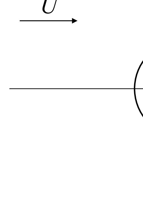
Figure 1: A pair of vortices behind a circular cylinder in a uniform stream.

We consider the motion of a pair of point vortices of same strength and opposite polarities around a circular cylinder of radius $a$ and in the presence of a uniform stream of velocity $U$, as illustrated in Fig. 1. It is convenient to work in the complex $z$-plane, where $z=x+iy$, and place the center of the cylinder at the origin. The upper and lower vortices are located at positions $z_{1}=x_{1}+iy_{1}$ and $z_{2}=x_{2}+iy_{2}$, respectively. The complex potential $w(z)=\phi(x,y)+i\psi(x,y)$, with $\phi$ being the velocity potential and $\psi$ the stream function, is given by milne

$$w(z)=U\left(z+\frac{a^{2}}{z}\right)+\frac{\Gamma}{2\pi i}\ln\frac{z-z_{1}}{z-{a^{2}}/{\bar{z}_{1}}}-\frac{\Gamma}{2\pi i}\ln\frac{z-z_{2}}{z-{a^{2}}/{\bar{z}_{2}}},$$ (1)

where $\Gamma$ is the circulation of the vortex at $z_{1}$ and bar denotes complex conjugation. In Eq. (1), the first two terms represent the incoming flow and its image (a doublet at the origin) with respect to the cylinder, the third term gives the contributions to the complex potential from the upper vortex and its image, and similarly the last term contains the contributions from the lower vortex and its image. As can be inferred from Fig. 1, a necessary condition for a steady configuration to exist is that the upper (lower) vortex be of negative (positive) circulation, hence only the case $\Gamma<0$ is of interest to us here.

In dimensionless variables

$$z^{\prime}=\frac{z}{a},\quad t^{\prime}=\frac{U}{a}t,\quad w^{\prime}=\frac{w}{Ua},\quad\kappa=-\frac{\Gamma}{2\pi Ua}>0,$$ (2)

the complex potential (1) becomes

$$w(z)=z+\frac{1}{z}+i\kappa\ln\frac{(z-{z_{1}})\left(1-\bar{z}_{2}z\right)}{(z-z_{2})\left(1-\bar{z}_{1}z\right)},$$ (3)

where the prime notation has been dropped. According to standard theory of point vortices in an inviscid fluid, any given vortex moves with the velocity of the flow computed at the position of that vortex, excluding its own contribution to the flow. It then follows from Eq. (3) that the velocity ${\bf u}_{1}=(u_{1},v_{1})$ of the vortex located at $z_{1}$ is given by

$$u_{1}-iv_{1}=1-\frac{1}{z_{1}^{2}}-i\kappa\left(\frac{1}{z_{1}-z_{2}}-\frac{\bar{z}_{1}}{1-z_{1}\bar{z}_{1}}+\frac{\bar{z}_{2}}{1-z_{1}\bar{z}_{2}}\right),$$ (4)

or more explicitly

$$u_{1}=1-\frac{x_{1}^{2}-y_{1}^{2}}{r_{1}^{4}}-\kappa \left(\frac{y_{1}-y_{2}}{r_{1}^{2}+r_{2}^{2}-2(x_{1}x_{2}+y_{1}y_{2})}+\frac{y_{1}}{r_{1}^{2}-1}-\frac{y_{1}r_{2}^{2}-y_{2}}{1+r_{1}^{2}r_{2}^{2}-2(x_{1}x_{2}+y_{1}y_{2})}\right),$$ (5a)

$$v_{1}=-2\frac{x_{1}y_{1}}{r_{1}^{4}}+\kappa \left(\frac{x_{1}-x_{2}}{r_{1}^{2}+r_{2}^{2}-2(x_{1}x_{2}+y_{1}y_{2})}+\frac{x_{1}}{r_{1}^{2}-1}-\frac{x_{1}r_{2}^{2}-x_{2}}{1+r_{1}^{2}r_{2}^{2}-2(x_{1}x_{2}+y_{1}y_{2})}\right),$$ (5b)

where $r_{i}^{2}=x_{i}^{2}+y_{i}^{2}$, $i=1,2$. The velocity ${\bf u}_{2}=(u_{2},v_{2})$ of the second vortex is obtained by simply interchanging the indexes $1\leftrightarrow 2$ in Eq. (5) and letting $\kappa\to-\kappa$.

III Dynamics on the Symmetric Subspace

It is not difficult to see from Eq. (5) that if the vortices are initially placed at positions symmetrically located with respect to the centerline, i.e., $z_{2}(0)=\overline{z}_{1}(0)$, then this symmetry is preserved for all later times, i.e., $z_{2}(t)=\overline{z}_{1}(t)$ for $t>0$. In this section, we study the dynamics within this invariant symmetric subspace, where the motion of the lower vortex is simply the mirror image of that of the upper vortex with respect to the centerline. Symmetry can be enforced experimentally by placing a splitter plate behind the cylinder in the center plane of the wake foeppl ; roshko .

With $x_{2}=x_{1}$ and $y_{2}=-y_{1}$, Eq. (5) reduces to

$$u=1-\frac{x^{2}-y^{2}}{r^{4}}+\kappa y\left[\frac{r^{2}+1}{(r^{2}-1)^{2}+4y^{2}}-\frac{1}{r^{2}-1}-\frac{1}{2y^{2}}\right],$$ (6a)

$$v=-2\frac{xy}{r^{4}}-\kappa x\left[\frac{r^{2}-1}{(r^{2}-1)^{2}+4y^{2}}-\frac{1}{r^{2}-1}\right].$$ (6b)

Here, the subscripts have been dropped with the understanding that in the remainder of the section we restrict our attention to the upper vortex.

III.1 Hamiltonian dynamics and phase portrait

As is well known, the equations of motion for point vortices in a two-dimensional inviscid flow, first derived by Kirchhoff, can be formulated as a Hamiltonian system saffman ; vvd . The dynamics of point vortices in the presence of closed, rigid boundaries was shown by Lin lin1941 to be also Hamiltonian with the same canonical sympletic structure as in the absence of boundaries. For a vortex pair placed in a uniform stream around a circular cylinder, the phase space is four-dimensional and has a two-dimensional (2D) invariant subspace corresponding to symmetric orbits. The Hamiltonian restricted to the 2D symmetric subspace is given by zannetti

$$H(x,y)=y\left(1-\frac{1}{r^{2}}\right)-\frac{\kappa}{2}\ln\frac{y(r^{2}-1)}{\sqrt{(r^{2}-1)^{2}+4y^{2}}}.$$ (7)

The corresponding dynamical equations

$$\dot{x}=\frac{\partial H}{\partial y},\quad\dot{y}=-\frac{\partial H}{\partial x},$$ (8)

where dot denotes time derivative, yield Eq. (6) upon identifying $(u,v)$ with $(\dot{x},\dot{y})$.

A phase portrait of this Hamiltonian system for $\kappa=45/32$ is presented in Fig. 2, where the curves shown are (unevenly spaced) level sets of the Hamiltonian (7). [For convenience, these curves were obtained from a direct numerical integration of Eq. (6).] A detailed description of the main features of this phase portrait will be given below, starting with an analysis of the various equilibrium points and their stability. The related problem of the symmetric “moving Föppl system,” where the cylinder advances through the fluid followed by the vortex pair, was recently considered by Shashikanth et al. marsden , but there the phase portrait shashi2006 is quite different from the one shown in Fig. 2, because of the additional degrees of freedom related to the velocity of the moving cylinder.

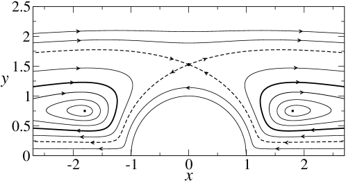
Figure 2: Phase portrait for the symmetric Föppl system with $\kappa=45/32$. The isolated black dots are the Föppl equilibria. The dashed curves are the stable and unstable branches of the separatrix associated with the equilibrium point on the normal line, and the thick solid lines are the homoclinic loops of the equilibrium point at infinity; see text.

III.2 Equlibrium points

The equilibrium positions for the vortex are obtained by setting $u=v=0$ in Eq. (6). Three types of equilibrium points can be identified.

III.2.1 Föppl equilibria

The locus of possible equilibrium positions $(x_{0},y_{0})$ for the upper vortex found by Föppl foeppl is the curve

$$r_{0}^{2}-1=2r_{0}y_{0},$$ (9)

with corresponding strength

$$\kappa=\frac{(r_{0}^{2}+1)(r_{0}^{2}-1)^{2}}{r_{0}^{5}}.$$ (10)

Along the Föppl curve (9), the vortex strength increases with distance from the center of the cylinder and diverges linearly for $r_{0}\to\infty$. For the equilibrium point on the edge of the cylinder ($r_{0}\to 1$), the strength vanishes. Notice that Eq. (9) yields two branches of solution: one in which the vortex pair is behind the cylinder ($x_{0}>0$) and the other where the vortex pair is in front of the cylinder ($x_{0}<0$). The former case models the formation of vortex eddies behind a cylinder in a uniform stream and was the primary motivation of Föppl’s original study foeppl . The latter case has attracted far less attention because it is not usually observed in experiments. We note, however, that recirculating eddies are observed in front of a circular cylinder near a plane boundary when the gap between the cylinder and the plane is sufficiently small lin . In this context, the Föppl equlibrium upstream of the cylinder may eventually be relevant for flows around a half-cylinder placed on a plane wall (or for the closely related situation where a splitter plate is attached to the front of the cylinder), although we are unaware of specific experiments in this setting.

III.2.2 Equilibria on the normal line

This corresponds to the upper vortex being located on the line bisecting the cylinder perpendicularly to the incoming flow weihs , that is,

$$x=0,\qquad y=b,\qquad b>1,$$ (11)

with strength

$$\kappa=\frac{2(b^{2}-1)(b^{2}+1)^{2}}{b(b^{4}+4b^{2}-1)}.$$ (12)

As in the Föppl solution, the strength tends to zero when the edge of the cylinder is reached ($b\to 1$) and diverges linearly with distance from the center of the cylinder. At large distances, the vortex strength for this equilibrium is about twice that of a Föppl pair located at the same distance from the origin.

III.2.3 Equilibrium at infinity

Equation (6) also yields equilibrium points at the positions

$$x=\pm\infty,\qquad y_{\infty}=\frac{\kappa}{2}.$$ (13)

To the best of our knowledge, the existence of this additional equilibrium point at infinity was not noted before. Its physical origin, however, can be easily understood, as it corresponds to the equilibrium configuration for a vortex pair placed in a uniform stream (without the cylinder). At points infinitely far from the cylinder, the flow induced by the image system (inside the cylinder) becomes negligible and hence a stationary configuration is possible if the vortices with given circulation $\pm\kappa$ are placed at the appropriate distance ($=\kappa$) from each other.

III.3 Stability analysis

The linear stability analysis of the equilibria described above is presented next, together with a discussion of the nonlinear stability of the Föppl equilibrium.

III.3.1 Föppl equilibria

Consider a perturbation of the Föppl equilibrium (9) parameterized as: $z=z_{0}+{\Delta z}$, where ${\Delta z}=\xi+i\eta$, with $\xi$ and $\eta$ being infinitesimal (real) quantities. Linearization of Eq. (6) then yields the following dynamical system

$$\left(\begin{array}[]{c}\dot{\xi}\cr\dot{\eta}\end{array}\right)=A\left(\begin{array}[]{c}{\xi}\cr{\eta}\end{array}\right),$$ (14)

where the matrix $A$ reads

$$A_{11}=-A_{22}=-\frac{x_{0}(r_{0}^{4}-3r_{0}^{2}+2)}{r_{0}^{8}},$$ (15)

$$A_{12}=\frac{4r_{0}^{8}+5r_{0}^{6}+2r_{0}^{4}-5r_{0}^{2}+2}{2r_{0}^{9}},$$ (16)

$$A_{21}=-\frac{2x_{0}^{2}(r_{0}^{4}+r_{0}^{2}+2)}{r_{0}^{7}(r_{0}^{2}+1)}.$$ (17)

Its eigenvalues $\lambda$ are given by

$$\lambda^{2}=-\frac{3r_{0}^{6}+5r_{0}^{4}+13r_{0}^{2}-5}{r_{0}^{10}}<0,$$ (18)

for $r_{0}>1$. The eigenvalues are thus purely imaginary, and not a complex pair with negative real part as found by Föppl foeppl . In other words, the Föppl equilibrium is a center and not a stable focus. Our equation (18) agrees with the expression for the eigenvalues of the symmetric modes obtained in Ref. [7] from the linearization of the full 4D dynamical system. As can be seen from Fig. 2, the Föppl solution is in fact a nonlinearly stable center, meaning that when the vortex is displaced from its equilibrium position by a small (but finite) amount, it executes a periodic motion around that point, corresponding to the closed orbits in the figure. This periodic motion around the Föppl equilibrium has been observed in numerical simulations of the model carried out by de Laat and Coene laat . Note that since the eigenvalues given in Eq. (18) do not depend explicitly on the coordinate $x_{0}$, it follows that the two Föppl equilibria, downstream and upstream of the cylinder, have identical stability properties, as is evident from Fig. 2. This means, in particular, that if vorticity can be generated upstream of the cylinder then stationary recirculating eddies could form in front of the cylinder—a situation observed, for instance, in flows around a cylinder placed above a plane wall lin .

III.3.2 Equilibria on the normal line

Linearization of Eq. (6) around the equilibrium point $z=ib$ yields for the matrix $A$:

$$A_{11}=A_{22}=0,$$ (19)

$$A_{12}=\frac{b^{8}+10b^{6}-8b^{4}+14b^{2}-1}{b^{3}(b^{2}-1)(b^{4}+4b^{2}-1)},$$ (20)

$$A_{21}=\frac{2(b^{2}-1)(3b^{2}-1)}{b^{3}(b^{4}+4b^{2}-1)}.$$ (21)

The eigenvalues $\lambda$ of this matrix are determined by

$$\lambda^{2}=\frac{2\left(3b^{2}-1\right)\left(b^{8}+10b^{6}-8b^{4}+14b^{2}-1\right)}{b^{6}(b^{4}+4b^{2}-1)^{2}}>0,$$ (22)

which yields a pair of real eigenvalues, $\lambda_{\pm}=\pm\sqrt{\lambda^{2}}$. The equilibrium point on the normal line is therefore a saddle, having a stable and unstable direction, as is also evident from the phase portrait shown in Fig. 2. The eigenvectors ${\bf w}_{\pm}$ associated with the eigenvalues $\lambda_{\pm}$, respectively, read

$${\bf w}_{\pm}=\left(\begin{array}[]{c}\pm\sqrt{A_{12}/A_{21}}\cr 1\end{array}\right).$$ (23)

Although it was known from numerical simulations laat that the equilibrium point on the normal line is unstable (against generic symmetric perturbations), it seems that an explicit linear stability analysis for this case was not carried out before, perhaps because these equilibria were not considered physically relevant since they are not observed in experiment foeppl . However, when the full nonlinear dynamics is considered, the stable and unstable eigendirections ${\bf w}_{\pm}$ give origin to the respective stable and unstable separatrices, indicated by the dashed curves in Fig. 2. In this sense, the existence of an equilibrium point on the normal line is dynamically felt by a vortex even if it is placed far from this “unphysical” equilibrium.

III.3.3 Equilibrium at infinity

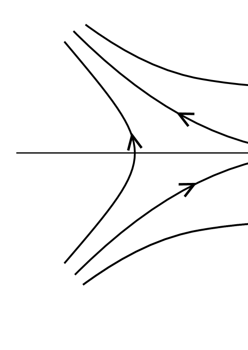
Figure 3: Trajectories near a nilpotent saddle.

The matrix $A$ of the linearized system around the equilibrium point at infinity is given by

$$A=-\frac{2}{\kappa}\left(\begin{array}[]{cc}0&1\cr 0&0\end{array}\right),$$ (24)

which is nilpotent and has two zero eigenvalues. To study the stability of this equilibrium point, one needs to examine the nonlinear contributions. To this end, we note that for $|x|\to\infty$ and $y\approx y_{\infty}$, Eq. (6b) assumes the form

$$\dot{y}=-\frac{\kappa}{x^{3}}.$$ (25)

It then follows from a theorem in ordinary differential equations perko that, in view of the cubic term in Eq. (25), the equilibrium point is a degenerate or nilpotent saddle abraham , for which the two eigenvectors are the same. The behavior of trajectories in the neighborhood of a generic nilpotent saddle is illustrated in Fig. 3. The behavior near the nilpotent saddle at $x=\pm\infty$ and $y=y_{\infty}$ can be described as follows. A vortex placed very far downstream and below (above) the line $y=y_{\infty}$ will move away from (towards) the equilibrium point at $x=\infty$. Similarly, a vortex placed very far upstream will move away from (towards) the equilibrium point at $x=-\infty$ if $y>y_{\infty}$ ($y<y_{\infty}$).

The stable and unstable separatrices associated with the nilpotent saddle at infinity form two homoclinic loops abraham , called nilpotent saddle loops, which are indicated in Fig. 2 by thick solid lines and correspond to the level curves passing through this equilibrium point:

$$H(x,y)=H(\pm\infty,y_{\infty})=\frac{\kappa}{2}\left(1-\ln\frac{\kappa}{2}\right).$$ (26)

The nilpotent saddle loops encircle the Föppl equilibria and define their region of nonlinear stability, in the sense that vortex trajectories are closed for initial positions inside the loops and unbounded otherwise. In this way, the nilpotent saddle at infinity, which went unnoticed until now, allows us to fully characterize the nonlinear stability of the Föppl equilibrium.

For unbounded orbits, the long-time asymptotic behavior depends on the location of the vortex initial position with respect to the separatrices associated with the equilibrium point on the normal line. A vortex placed downstream of the cylinder between the nilpotent saddle loop and the separatrices of the equilibrium point on normal line will eventually be convected away by the free stream; see Fig. 2. In particular, if the vortex starts very far behind the cylinder at a position that is below the nilpotent saddle loop and above the stable separatrix, it first moves towards the cylinder, turns around the Föppl equilibrium, and is then “reflected” back to infinity. Even more surprising trajectories arise if the vortex is placed downstream below the stable separatrix, for it will be close enough to its image below the centerline to be able to overcome the cylinder and move off to infinity upstream. (A related phenomenon occurs in the inviscid coupled motion of a cylinder initially at rest and a vortex pair starting at infinity with no imposed background flow eames . When the cylinder is less dense than the fluid, it is found that if the vortices are released sufficiently above the centerline they reverse relative to the moving cylinder; otherwise, they move over and past the cylinder.) Unbounded trajectories for the Föppl system also result for initial positions upstream of the cylinder: i) if placed above the stable separatrix, the vortex moves downstream to infinity; and ii) if placed between the stable separatrix and the nilpotent saddle loop, the vortex goes around the Föppl equlibrium in front of the cylinder and returns to infinity upstream; see Fig. 2. It is again the hitherto unnoticed nilpotent saddle at infinity, together with the precise nature of the equilibrium point on the normal line, that allows us to go beyond linear stability analysis and capture the full phase portrait in the symmetric subspace.

We stress that closed orbits exist only when the flow is symmetric. Nonsymmetric perturbations inevitably cause the vortex pair to move off to infinity, as we demonstrate next.

IV Nonsymmetric Dynamics

In this section, the effect of antisymmetric perturbations on the equilibria of the Föppl system is studied. We begin by observing that the dynamics of two counter-rotating point vortices possesses a conjugation symmetry. To describe this symmetry, let $z_{1}(t;z_{1,0},z_{2,0})$ and $z_{2}(t;z_{1,0},z_{2,0})$ denote the trajectories of the upper and lower vortices, respectively, with initial positions $z_{1,0}$ and $z_{2,0}$. For the dynamical system defined by Eq. (5) and the corresponding equation for the second vortex, one can verify that the following relations hold

$$z_{1}(t;\overline{z}_{2,0},\overline{z}_{1,0})=\overline{z_{2}(t;z_{1,0},z_{2,0})},$$ (27a)

$$z_{2}(t;\overline{z}_{2,0},\overline{z}_{1,0})=\overline{z_{1}(t;z_{1,0},z_{2,0})}.$$ (27b)

In other words, for any given pair of initial positions, $z_{1,0}$ and $z_{2,0}$, there exists a “conjugate pair” of initial positions, $\overline{z}_{2,0}$ and $\overline{z}_{1,0}$, such that the vortex trajectories of the first pair are the complex conjugate of those of the second pair.

Any perturbation of a vortex-pair equilibrium can be written as the superposition of a symmetric perturbation and an antisymmetric one. To be precise, antisymmetric perturbations are of the form

$$z_{1}=z_{0}+\Delta z,\qquad z_{2}=\overline{z}_{0}-\overline{\Delta z},$$ (28)

where $z_{0}$ denotes a generic equilibrium point and ${\Delta z}=\xi+i\eta$. Since the antisymmetric subspace of the full 4D phase space is invariant under linear dynamics, we can focus on the upper vortex in carrying out our linear stability analysis.

IV.1 Föppl equilibria

Linearization of Eq. (5) around the Föppl equilibrium (9) with respect to antisymmetric perturbations (28) yields

$$\left(\begin{array}[]{c}\dot{\xi}\cr\dot{\eta}\end{array}\right)=B\left(\begin{array}[]{c}{\xi}\cr{\eta}\end{array}\right),$$ (29)

where the matrix $B$ is given by

$$B_{11}=-B_{22}=\frac{x_{0}\left(r_{0}^{4}+3r_{0}^{2}-2\right)}{r_{0}^{8}},$$ (30)

$$B_{12}=\frac{3r_{0}^{6}-5r_{0}^{2}+2}{2r_{0}^{9}},$$ (31)

$$B_{21}=\frac{4r_{0}^{8}+3r_{0}^{6}-4r_{0}^{4}-5r_{0}^{2}+2}{2r_{0}^{9}}.$$ (32)

This matrix has a pair of real eigenvalues, $\lambda_{\pm}=\pm\sqrt{\lambda^{2}}$, where

$$\lambda^{2}=\frac{3r_{0}^{6}+3r_{0}^{4}-3r_{0}^{2}+1}{r_{0}^{10}}.$$ (33)

The Föppl equilibrium is therefore a saddle with respect to antisymmetric perturbations, while it is a center with respect to symmetric perturbations, as seen earlier. That is, the Föppl equilibrium is a saddle-center of the full 4D dynamical system hs . We note in passing that, although Föppl obtained a pair of real eigenvalues for the case of antisymmetric perturbations, his original formulae for the eigenvalues are in error footnote . Our expression (33) is in agreement with the eigenvalues of the skew-symmetric modes obtained by Smith smith from the linearization of the full dynamical system. The eigenvectors ${\bf w}_{\pm}$ associated with the eigenvalues $\lambda_{\pm}$ are readily computed, with the result

$${\bf w}_{\pm}=\left(\begin{array}[]{c}(\lambda_{\pm}+B_{11})/B_{21}\cr 1\end{array}\right).$$ (34)

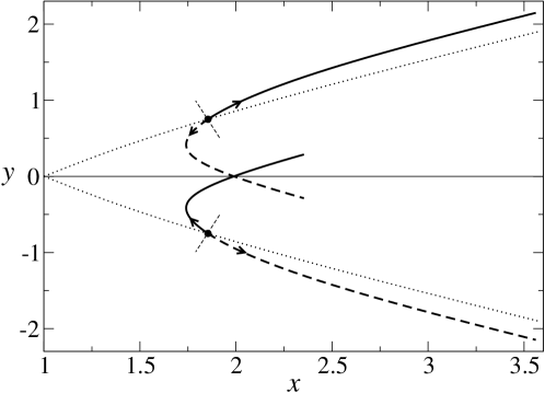
Figure 4: Vortex trajectories for antisymmetric perturbations of the Föppl equilibrium for $\kappa=45/32$, in which case $x_{0}=\sqrt{55}/4$ and $y_{0}=\pm 3/4$ (black dots). The solid and dashed curves are the trajectories starting along the unstable directions ${\bf w}_{+}$ and $-{\bf w}_{+}$, respectively, while the short straight lines indicate the axes defined by the stable direction ${\bf w}_{-}$. The dotted lines represent the loci of the Föppl equilibria.

In Fig. 4, we show in solid curves the pair of vortex trajectories obtained by slightly displacing the vortices from their equilibrium positions in the directions defined by the unstable eigenvector ${\bf w_{+}}$, while the trajectories obtained by slightly displacing the vortices in the opposite directions are shown in dashed curves. The latter pair of trajectories is the complex conjugate of the former by conjugation symmetry. Note that for the first pair of trajectories, the lower vortex initially moves towards the centerline and upstream, while the upper vortex moves away from the centerline and downstream. At later times, the vortex pair moves off to infinity with the lower vortex trailing behind the upper vortex. For the second pair of trajectories, the upper and lower vortices switch role; see Fig. 4. In the flow of a real fluid past a cylinder, the two basic instabilities associated with displacements along the unstable directions $\pm{\bf w_{+}}$ happen alternately and constitute the origin of vortex shedding that leads to the formation of the Karman vortex street tang . In like manner, the suppression of vortex shedding by placing a splitter plate behind the cylinder roshko ; roshko2 is consistent with the fact that the Föppl equlibrium is nonlinearly stable with respect to symmetric perturbations; see Sec. V for further discussions on vortex shedding and its suppression by a splitter plate.

For small, generic antisymmetric perturbations, the vortices move along trajectories that follow closely the ones depicted in Fig. 4. Whether a vortex pair eventually moves up or down is determined by the initial position of the upper vortex relative to the stable direction ${\bf w}_{-}$, which is indicated in Fig. 4 by the short straight line passing through the Föppl equilibrium. If the initial position of the upper vortex is to the right (left) of the stable direction, then the vortex pair asymptotically moves upwards (downwards). This explains the behavior seen in the numerical simulations reported in Ref. [25], where nearby initial positions around the Föppl equilibrium were found to lead to close-by trajectories.

Since any degree of antisymmetry in the initial perturbation causes the vortex pair to move off to infinity, the Föppl equilibrium is unstable under generic perturbations. As an example, Fig. 5 shows vortex trajectories obtained by displacing the Föppl pair (at $r_{0}=2$) by the amounts $\Delta z_{1}=\Delta z_{2}=-0.25+i0.005$. During the linear stage, the trajectories are a superposition of a symmetric orbit and a growing mode associated with the antisymmetric component of the perturbation, which ultimately leads to asymptotic trajectories with the vortices moving parallel to each other.

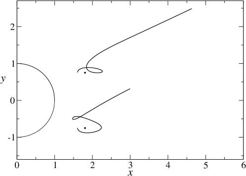
Figure 5: Trajectories resulting from a generic perturbation ${\Delta z}_{1}=\Delta z_{2}=-0.25+i0.005$ of the Föppl pair at $r_{0}=2$ (black dots).

IV.2 Equilibria on the normal line

For antisymmetric perturbations of the equilibrium (11) on the normal line, the matrix $B$ assumes the form

$$B_{11}=B_{22}=0,$$ (35)

$$B_{12}=\frac{2\left(3b^{6}+b^{4}+5b^{2}-1\right)}{b^{3}(b^{2}-1)\left(b^{4}+4b^{2}-1\right)},$$ (36)

$$B_{21}=\frac{b^{2}-1}{b^{3}},$$ (37)

with eigenvalues $\lambda$ given by

$$\lambda^{2}=\frac{2\left(3b^{6}+b^{4}+5b^{2}-1\right)}{b^{6}\left(b^{4}+4b^{2}-1\right)}>0.$$ (38)

This yields a pair of real eigenvalues, $\lambda_{\pm}=\pm\sqrt{\lambda^{2}}$, with respective eigenvectors:

$${\bf w}_{\pm}=\left(\begin{array}[]{c}\pm\sqrt{B_{12}/B_{21}}\cr 1\end{array}\right).$$ (39)

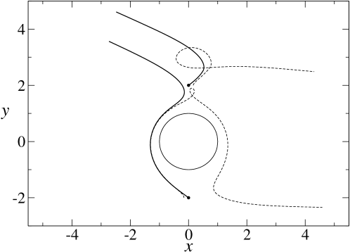
Figure 6: Vortex trajectories (solid curves) associated with the unstable direction ${\bf w}_{+}$ of the equilibrium at $z=\pm 2i$ (black dots). The dashed curves are trajectories resulting from the antisymmetric perturbation $\Delta z=0.16$.

In Fig. 6, we show the vortex trajectories (solid curves) obtained by slightly displacing the vortices from their equilibrium position along the unstable direction ${\bf w}_{+}$ for $b=2$. The initial motion here is somewhat similar to what is seen for a Föppl pair, in the sense that one vortex moves upstream towards the centerline and the other moves downstream away from the centerline. The main difference is that for later times, the vortices now end up moving upstream. The long-time dynamics in this case is also more sensitive on the initial conditions: for somewhat larger perturbations, the vortices are eventually carried away by the free stream. An example where this happens is indicated by the dashed curves in Fig. 6, which represent the vortex trajectories for the antisymmetric perturbation $\Delta z=0.16$.

As already argued in Sec. III.3.2, although the equilibrium point on the normal line is not directly observed in experiments, it is important to know its instability properties under both symmetric and antisymmetric perturbations. This knowledge contributes to a better understanding not only of the full nonlinear dynamics of the Föppl system but also of more general flows, such as the case of stationary vortex patches above and below the cylinder in a uniform stream, where similar unstable modes are observed elcrat2 .

V Discussion and Conclusions

In this paper, we have investigated a two-dimensional vortex model for the formation of recirculating eddies behind a fixed cylinder placed on a uniform stream. The model, which was first introduced by Föppl foeppl almost a century ago, has two main simplifying assumptions: i) the fluid is treated as inviscid and hence the flow is potential, and ii) the size of the vortex core is neglected and so the vortices are considered to be point-like. In spite of these simplifications, the model is known to be in qualitative agreement with real flows past a cylinder, as was already pointed out by Föppl in his original paper. Several novel features of the Föppl model have been obtained in the present work, which help one to better understand the basic dynamics of vortex shedding behind a cylinder.

In real flows, governed by the Navier-Stokes equations, stationary vortices behind a cylinder are formed at moderate Reynolds number ($Re<50$). As the Reynolds number increases past $Re\approx 50$, the configuration loses its symmetry and becomes unstable. New vortices then start to form alternately on both sides of the cylinder, while the vortices further downstream break away and develop into a Karman vortex street, as described by Föppl foeppl . It has been argued by Roshko roshko that “possibly the breaking away should be regarded as primary, resulting in asymmetry.” The analysis presented in Sec. IV.1 makes it clear that the reverse scenario is more plausible: the asymmetrical disturbances induce the instability of the vortex pair which then breaks away from the cylinder. As vorticity is continuously generated from the separated boundary layer on both sides of the cylinder, new vortices are formed and alternately shed into the far wake of the cylinder according to the unstable modes shown in Fig. 4. Direct numerical simulations (DNS) of two-dimensional flows past a cylinder performed by Tang and Aubry tang have confirmed that the mechanism for the instability of the symmetric eddies in real flows is qualitatively described by the instability of the point-vortex model.

It is experimentally observed roshko ; roshko2 that vortex shedding is suppressed if a splitter plate is installed behind the cylinder in the center plane of the wake. The presence of the splitter plate tends to enforce symmetry of the flow with respect to the centerline, thus effectively reducing the appearance of antisymmetric disturbances behind the cylinder. The suppression of vortex shedding in this case is thus entirely consistent with the fact that the Föppl equilibria of the vortex-point model is nonlinearly stable against symmetric perturbations and that vortex shedding is induced by unstable antisymmetric modes, as discussed above. This scenario has been confirmed by DNS of flows past a cylinder with symmetry imposed along the centerline recently performed by Kumar et al. kumar . The problem of stationary configurations for vortex flows past a cylinder with patches of constant vorticity has also been studied numerically by Elcrat et al. elcrat1 ; elcrat2 . These authors found two families of solutions, representing desingularized versions of the Föppl and the normal equilibria, respectively, which have the same stability properties as the corresponding point-vortex equilibria.

In conclusion, we have seen that the Föppl model, where a pair of counter-rotating point vortices move around a circular cylinder in the presence of a uniform stream, is a rich nonlinear dynamical system whose features—notably its stability properties—bear a direct relevance to our understanding of the vortex shedding mechanism in real flows. The results obtained here should, in principle, carry over to more general geometries, such as vortex motion around a plate or around a cylinder with noncircular cross section.

- (1) M. M. Zdravkovich, Flow around circular cylinders, Vol. 1: Fundamentals; Vol. 2: Applications (Oxford University Press, Oxford, 1997).
- (2) B. M. Sumer and J. Fredsøe, Hydrodynamics around cylindrical structures (World Scientific, Singapore, 2006).
- (3) P. G. Saffman, Vortex Dynamics (Cambridge University Press, Cambridge, 1992).
- (4) J.-Z. Wu, H.-Y. Ma, and M.-D. Zhou, Vorticity and Vortex Dynamics (Springer, Berlin, 2006).
- (5) L. Föppl,“Wirbelbewegung hinter einem Kreiszylinder,” Sitzb. Bayer. Akad. Wiss. 1, 1 (1913).
- (6) S. Tang and N. Aubry, “On the symmetry breaking instability leading to vortex shedding,” Phys. Fluids 9, 2550 (1997).
- (7) A. C. Smith, “On the stability of Föppl’s vortices,” J. Appl. Mech. 70, 610 (1973).
- (8) I. Soibelman (private communication); see also page 43 of Ref. [3].
- (9) J. Cai, F. Liu, and S. Luo, “Stability of a vortex pair behind two-dimensional bodies,” AIAA Paper 2001-2844 (2001).
- (10) A. Roshko, “On the development of turbulent wakes from vortex streets,” NACA Technical Report 1191, US Government Printing Office, Washington DC (1954).
- (11) A. Roshko, “Experiments on the flow past a circular cylinder at very high Reynolds number,” J. Fluid Mech. 10, 345 (1961).
- (12) J. Cai, F. Liu, and S. Luo, “Stability of symmetric vortices in two dimensions and over three-dimensional slender conical bodies,” J. Fluid Mech. 480, 65 (2003).
- (13) T. W. G. D. de Laat and R. Coene, “Two-dimensional vortex motion in the cross-flow of a wing-body configuration,” J. Fluid Mech. 305, 93 (1995).
- (14) D. D. Seath, “Equilibirum vortex positions,” J. Spacecraft 8, 72 (1971).
- (15) D. Weihs and M. Boasson, “Multiple equilibrium vortex positions in symmetric shedding from slender bodies,” AIAA Journal 17, 213 (1979).
- (16) K. G. Miller, “Stationary cornex vortex configurations,” Z. Angew. Math. Phys. 47, 39 (1996).
- (17) B. Protas, “Higher-order Föppl models of steady wake flows,” Phys. Fluids 18, 117109 (2006).
- (18) B. N. Shashikanth, J. E. Marsden, J. W. Burdick, and S. D. Kelly, “The Hamiltonian structure of a two-dimensional rigid circular cylinder interacting dynamically with point vortices,” Phys. Fluids 14, 1214 (2002). (Erratum: Phys. Fluids 14, 4099 (2002).)
- (19) B. N. Shashikanth, “Symmetric pairs of point vortices interacting with a neutrally buoyant two-dimensional circular cylinder,” Phys. Fluids 18, 127103 (2006).
- (20) A. V. Borisov, I. S. Mamaev, and S. M. Ramodanov, “Dynamic interaction of point vortices and a two-dimensional cylinder,” J. Math. Phys. 48, 065403 (2007).
- (21) S. Tang and N. Aubry, “Suppression of vortex shedding inspired by a low-dimensional model,” J. Fluids Struct. 14, 443 (2000).
- (22) B. Protas, “Linear feedback stabilization of laminar vortex shedding based on a point vortex model,” Phys. Fluids 16, 4473 (2004).
- (23) B. Protas, “Center manifold analysis of a point vortex model of vortex shedding with control,” Physica D 228, 179 (2007).
- (24) J. Cai, F. Liu, and S. Luo, “Stability of symmetric and asymmetric vortex pairs over slender conical wings and bodies,” Phys. Fluids 16, 424 (2004).
- (25) D. H. Bridges, “Toward a theoretical description of vortex wake asymmetry,” Prog. Aerosp. Sci. 46, 62 (2010).
- (26) A. Elcrat, B. Fornberg, M. Horn, and K. Miller, “Some steady vortex flows past a circular cylinder,” J. Fluid Mech. 409, 13 (2000).
- (27) A. Elcrat, B. Fornberg, and K. Miller, “Stability of vortices in equilibrium with a cylinder,” J. Fluid Mech. 544, 53 (2005).
- (28) B. Protas, “Vortex dynamics models in flow control problems,” Nonlinearity 21, R203 (2008).
- (29) L. M. Milne-Thomson, Theoretical Hydrodynamics, 5th ed. (Dover, New York, 1996).
- (30) C. C. Lin, “On the motion of vortices in two dimensions–I and II,” Proc. Natl. Acad. Sci. U.S.A. 27, 570 (1941).
- (31) L. Zannetti, “Vortex equilibrium in flows past bluff bodies,” J. Fluid Mech. 562, 151 (2006).
- (32) W-J. Lin, C. Lin, S-C. Hsieh, and S. Dey, “Flow characterization around a circular cylinder placed horizontally above a plane boundary,” J. Eng. Mech. 135, 697 (2009).
- (33) L. Perko, Differential Equations and Dynamical Systems (Springer, New York, 1991).
- (34) M. Han, C. Shu, J. Yang, and A. C.-L. Chian, “Polynomial Hamiltonian systems with a nilpotent critical point,” Adv. Space Res. 46, 521 (2010).
- (35) I. Eames, M. Landeryou, and J. B. Flór, “Inviscid coupling between point symmetric bodies and singular distributions of vorticity,” J. Fluid Mech. 589, 33 (2007).
- (36) L. M. Lerman and Y. L. Umanskiy, Four-dimensional Integrable Hamiltonian Systems with Simple Singular Points (American Mathematical Society, Providence, 1998).
- (37) The formula for the matrix element given in Eq. (17) of Ref. [5], which corresponds to the matrix element in our Eq. (32), is in error.
- (38) B. Kumar, J. J. Kottaram, A. K. Sing, and S. Mittal, “Global stability of flow past a cylinder with centreline symmetry,” J. Fluid Mech. 632, 273 (2009).