A population Monte Carlo scheme with transformed weights and its application to stochastic kinetic models

Abstract

This paper addresses the problem of Monte Carlo approximation of posterior probability distributions. In particular, we have considered a recently proposed technique known as population Monte Carlo (PMC), which is based on an iterative importance sampling approach. An important drawback of this methodology is the degeneracy of the importance weights when the dimension of either the observations or the variables of interest is high. To alleviate this difficulty, we propose a novel method that performs a nonlinear transformation on the importance weights. This operation reduces the weight variation, hence it avoids their degeneracy and increases the efficiency of the importance sampling scheme, specially when drawing from a proposal functions which are poorly adapted to the true posterior.

For the sake of illustration, we have applied the proposed algorithm to the estimation of the parameters of a Gaussian mixture model. This is a very simple problem that enables us to clearly show and discuss the main features of the proposed technique. As a practical application, we have also considered the popular (and challenging) problem of estimating the rate parameters of stochastic kinetic models (SKM). SKMs are highly multivariate systems that model molecular interactions in biological and chemical problems. We introduce a particularization of the proposed algorithm to SKMs and present numerical results.

1 Introduction

The problem of performing inference in high dimensional spaces appears in many practical applications. For example, it is of increasing interest in the biological sciences to develop new techniques that allow for the efficient estimation of the parameters governing the behavior of complex autoregulatory networks. The main difficulty often encountered when tackling this kind of problems is the design of numerical inference algorithms which are stable and have a guaranteed convergence also in high-dimensional spaces.

A very common strategy, which has been successfully applied in a broad variety of complex problems, is the Monte Carlo methodology. In particular, we have considered a recently proposed technique known as population Monte Carlo (PMC) Cappe04 , which is based on an iterative importance sampling approach. The aim of this method is the approximation of static probability distributions by way of discrete random measures consisting of samples and associated weights. The target distribution is often the posterior distribution of a set variables of interest, given some observed data.

The main advantages of the PMC scheme, compared to the widely established Markov chain Monte Carlo (MCMC) methodology, are the possibility of developing parallel implementations, the sample independence and the fact that an unbiased estimate is provided at each iteration, which avoids the need of a convergence period.

On the contrary, an important drawback of the importance sampling approach, and particulary of PMC, is that its performance heavily depends on the choice of the proposal distribution (or importance function) that is used to generate the samples and compute the weights. When the dimension of the variables of interest is large, or the target probability density function (pdf) is very sharp with respect to the proposal (this occurs when, e.g., the number of observations is high or when the prior distribution is uninformative), the importance weights degenerate leading to an extremely low number of representative samples. This problem is commonly known as weight degeneracy and is closely related to the “curse of dimensionality”. To the best of our knowledge, the degeneracy problem has not been successfully addressed so far in the PMC framework. The issue was already mentioned in the original paper Cappe04 , though, noting that the proposed scheme did not provide neither a stabilization of the so called effective sample size, nor of the variance of the importance weights.

The effort in the field of PMC algorithms has been mainly directed toward the design of efficient proposal functions. A recently proposed scheme for the proposal update is the mixture PMC technique Cappe08 , that models the importance functions as mixtures of kernels. Both the weights and the internal parameters of each mixture component are adapted along the iterations with the goal of minimizing the Kullback-Leiber divergence between the target density and the proposal. However, this scheme also suffers from degeneracy unless applied to very simple examples and the authors of Cappe08 propose to apply an additional Rao-Blackwellization scheme to mitigate the problems that appear in multidimensional problems.

Another recently proposed PMC scheme Djuric11 is based on the Gibbs sampling method and constructs the importance functions as alternating conditional densities. Thus, this method allows to sample efficiently from high-dimensional proposals. However, the importance weights still present severe degeneracy due to the extreme values of the likelihood function in high-dimensional spaces, unless the number of samples is extremely high. The technique is based on the multiple marginalized PMC, proposed in Bugallo09 , Shen10 .

In this paper we propose a novel PMC method, termed nonlinear PMC (NPMC). The emphasis is not placed on the proposal update scheme, which can be very simple (here we restrict ourselves to importance functions chosen as multivariate normal denisities whose parameters are adjusted along the iterations to match the moments of the latest approximation of the posterior distribution). The main feature of the technique is the application of a nonlinear transformation to the importance weights in order to reduce their variations. In this way, the efficiency of the sampling scheme is improved (specially when drawing from “poor” proposals) and, most importantly, the degeneracy of the weights is drastically mitigated even when the number of generated samples is relatively small. We show analytically that the approximate integrals computed using the transformed weights converge asymptotically to the true integrals.

In this work we have successfully applied the proposed methodology to two different problems where severe weight degeneracy is observed. The first example is a Gaussian mixture model, already discussed in Cappe04 . We have used this example to illustrate the degeneracy problem and for comparison of the original PMC scheme with the proposed methods. We provide numerical results that suggest that degeneracy of the importance weights takes places even in simple and low-dimensional problems, when the proposal pdf is wide with respect to the target. The proposed method clearly outperforms the original PMC scheme and provides a high number of representative samples and very accurate estimates of the variables of interest.

As a practical application, we have also applied the proposed algorithm to the popular (and challenging) problem of estimating the rate parameters in stochastic kinetic models Boys08 . Such models describe the time evolution of the population of a set of species or chemical reactions, which evolve according to a set of constant rate parameters, and present an autoregulatory behavior. This problem is currently of great interest in a broad diversity of biological and molecular problems, such as complex auto-regulatory gene networks.

We introduce a particularization of the generic NPMC algorithm to SKMs, which tackles the evaluation of the likelihood function (which can not be computed exactly) using a particle filter. As a simple and intuitive, yet physically meaningful example, we have obtained numerical results for the Lotka-Volterra model, also known as predator-prey model, consisting of two interacting species related by three reactions with associated unknown rates. The proposed method provides a very good performance also in this scenario, where standard PMC algorithms can be easily shown to fail.

The rest of the paper is organized as follows. In Section 2 we introduce some notation. In Section 3, we give a formal statement of the class of problems addressed in this paper. In Section 4, the population Monte Carlo algorithm is presented and a discussion of the weight degeneracy problem is provided. In section 5 the proposed algorithm is described. In section 6 we provide a theoretical convergence analysis of the new methodology. In section 7 we present numerical results on a Gaussian mixture model. We illustrate the effects of degeneracy and the performance of the proposed algorithms in this scenario. In Section 8, we describe the practical application of the proposed algorithm to the problem of estimating the constant rates of a stochastic kinetic model, and present numerical results. Section 9 is devoted to the conclusions.

2 Notation

In this section we introduce some notations that are used through the paper.

• All vectors are assumed to have column form. We denote them using boldface lower-case letters, e.g., $\boldsymbol{\theta}$, y, and its $k$-th scalar component is written as the corresponding normal-face letter with a subscript, e.g., $\theta_{k}$, $y_{k}$. Matrices are denoted by boldface upper-case letters, e.g., $\boldsymbol{\Sigma}$. $N$.

• We use $\mathbb{R}^{K}$, with integer $K\geq 1$, to denote the set of $K$-dimensional vectors with real entries.

• $B(\mathbb{R}^{K})$ is the set of bounded real functions over $\mathbb{R}^{K}$. In particular, the supremum norm of a real function $f:\mathbb{R}^{K}\rightarrow\mathbb{R}$ is denoted as $\|f\|_{\infty}=\sup_{\textbf{z}\in\mathbb{R}^{K}}|f(\textbf{z})|$ and $f\in B(\mathbb{R}^{K})$ when $\|f\|_{\infty}<\infty$.

• The target pdf of a PMC algorithm is denoted as $\pi$, the proposal density as $q$ and the rest of pdf’s as $p$.

• We write conditional pdf’s as $p(\textbf{y}|\boldsymbol{\theta})$, and joint densities as $p(\boldsymbol{\theta})=p(\theta_{1},\ldots,\theta_{K})$. This is an argument-wise notation, hence $p(\theta_{1})$ denotes the distribution of $\theta_{1}$, possibly different from $p(\theta_{2})$, which represents the distribution of $\theta_{2}$.

• The integral of a function $f$ with respect to a measure $\mu$ is denoted by the shorthand $(f,\mu)=\int f(\boldsymbol{\theta})\mu(d\boldsymbol{\theta})$. If the measure has a density $\pi$, i.e., $\mu(d\boldsymbol{\theta})=\pi(\boldsymbol{\theta})d\boldsymbol{\theta}$, then we also write $(f,\pi)=\int f(\boldsymbol{\theta})\pi(\boldsymbol{\theta})d\boldsymbol{\theta}$.

• $E_{p(\boldsymbol{\theta})}[f(\boldsymbol{\theta})]$ denotes expectation of the function $f$ with respect to the probability distribution with density $p(\boldsymbol{\theta})$.

• A sample from the distribution of the random vector $\boldsymbol{\theta}$ is denoted by $\boldsymbol{\theta}^{(i)}$. Sets of $M$ samples $\{\boldsymbol{\theta}^{(1)},\ldots,\boldsymbol{\theta}^{(M)}\}$ are denoted as $\{\boldsymbol{\theta}^{(i)}\}_{i=1}^{M}$.

• $\delta_{\theta^{(i)}}(d\boldsymbol{\theta})$ is the unit delta measure located at $\boldsymbol{\theta}=\boldsymbol{\theta}^{(i)}$.

• Unweighted samples are denoted with a tilde as $\left\{\tilde{\boldsymbol{\theta}}^{(i)}\right\}$, opposite to the corresponding weighted samples $\left\{\boldsymbol{\theta}^{(i)}\right\}$.

• For a random value $X$, $\mathbb{P}\{X<a\}$ denotes the probability of the event $X<a$.

• In the chemical representation the notation $\alpha x$ must not be interpreted as a product, but rather is read as “$\alpha$ molecules of species $x$”.

3 Problem Statement

Let $\boldsymbol{\theta}=\left[\theta_{1},\ldots,\theta_{K}\right]^{\top}$ be a vector of $K$ unobserved real random variables with prior density $p(\boldsymbol{\theta})$ and let $\textbf{y}=\left[y_{1},\ldots,y_{N}\right]^{\top}$ be a vector of $N$ real random observations related to $\boldsymbol{\theta}$ by way of a conditional pdf $p(\textbf{y}|\boldsymbol{\theta})$.

In this paper we address the problem of approximating the posterior probability distribution of $\boldsymbol{\theta}$, i.e., the distribution with density $p(\boldsymbol{\theta}|\textbf{y})$, using a random grid of $M$ points, $\{\boldsymbol{\theta}^{(i)}\}_{i=1}^{M}$, in the space of the random vector $\boldsymbol{\theta}$. Once the grid is generated, it is simple to approximate any moments of $p(\boldsymbol{\theta}|\textbf{y})$. For example, the posterior mean of $\boldsymbol{\theta}$ given the observations y may be approximated as

$$E_{p(\boldsymbol{\theta}|\textbf{y})}[\boldsymbol{\theta}]=\int\boldsymbol{\theta}p(\boldsymbol{\theta}|\textbf{y})d\boldsymbol{\theta}\approx\frac{1}{M}\sum_{i=1}^{M}\boldsymbol{\theta}^{(i)}.$$

Unfortunately, the generation of useful samples that represent the probability measure $p(\boldsymbol{\theta}|\textbf{y})d\boldsymbol{\theta}$ adequately when $K$ (or $N$) is large is normally a very difficult task. The main goal of this work is to devise and assess an efficient computational inference (Monte Carlo) methodology for the approximation of $p(\boldsymbol{\theta}|\textbf{y})d\boldsymbol{\theta}$ and its moments, i.e., expectations of the form $E_{p(\boldsymbol{\theta}|\textbf{y})}[f(\boldsymbol{\theta}|\textbf{y})]$, where $f:\mathbb{R}^{K}\rightarrow\mathbb{R}$ is some integrable function of $\boldsymbol{\theta}$.

4 Population Monte Carlo

4.1 Importance Sampling

One of the main applications of statistical Monte Carlo methods is the approximation of integrals of the form

$$(f,\pi)=\int f(\boldsymbol{\theta})\pi(\boldsymbol{\theta})d\boldsymbol{\theta},$$

where $f$ is a real, integrable function of $\boldsymbol{\theta}$ and $\pi(\boldsymbol{\theta})$ is some pdf of interest (often termed the target density). Given the random sample $\left\{\boldsymbol{\theta}^{(i)}\right\}_{i=1}^{M}$ we build a random discrete measure

$$\pi^{M}(d\boldsymbol{\theta})=\frac{1}{M}\sum_{i=1}^{M}\delta_{\boldsymbol{\theta}^{(i)}}(d\boldsymbol{\theta})$$

that enables a straightforward approximation $(f,\pi^{M})$ of $(f,\pi)$, namely

$$(f,\pi)\approx(f,\pi^{M})=\int f(\boldsymbol{\theta})\pi^{M}(d\boldsymbol{\theta})=\frac{1}{M}\sum_{i=1}^{M}f\left(\boldsymbol{\theta}^{(i)}\right).$$

Under mild assumptions, it can be shown that Robert04

$$\lim_{M\rightarrow\infty}(f,\pi^{M})=(f,\pi)\quad\mbox{a.s.}$$

However, in many practical cases it is not possible to sample from $\pi(\boldsymbol{\theta})$ directly. A common approach to overcome this difficulty is to apply an importance sampling (IS) procedure Robert04 . The key idea is to draw the samples $\{\boldsymbol{\theta}^{(i)}\}_{i=1}^{M}$ from a (simpler) proposal pdf, or importance function, $q(\boldsymbol{\theta})$, and then compute associated importance weights of the form

$$w^{(i)*}\propto\frac{\pi\left(\boldsymbol{\theta}^{(i)}\right)}{q\left(\boldsymbol{\theta}^{(i)}\right)},$$

which we subsequently normalize to yield

$$w^{(i)}=\frac{w^{(i)*}}{\sum_{j=1}^{M}w^{(j)*}},\qquad i=1,\ldots,M.$$

The integral $(f,\pi)$ is then approximated by the weighted sum

$$(f,\pi^{M})=\sum_{i=1}^{M}w^{(i)}f\left(\boldsymbol{\theta}^{(i)}\right).$$

The efficiency of an IS algorithm depends heavily on the choice of the proposal, $q(\boldsymbol{\theta})$. However, in order to ensure the asymptotic convergence of the approximation $(f,\pi^{M})$, when $M$ is large enough, it is sufficient to select $q(\boldsymbol{\theta})$ such that $q(\boldsymbol{\theta})>0$ whenever $\pi(\boldsymbol{\theta})>0$ Robert04 .

Finally, note that the computation of the normalized weights requires that both $\pi(\boldsymbol{\theta})$ and $q(\boldsymbol{\theta})$ can be evaluated up to a proportionality constant independent of $\boldsymbol{\theta}$. This requirement is a mild one, since in most problems it is possible to evaluate some function $h(\boldsymbol{\theta})\propto\pi(\boldsymbol{\theta})$.

4.2 Population Monte Carlo Algorithm

The population Monte Carlo (PMC) method Cappe04 is an iterative IS scheme that seeks to generate a sequence of proposal pdf’s $q_{\ell}(\boldsymbol{\theta})$, $\ell=1,\ldots,L$, such that every new proposal is closer (in some adequate sense to be defined) to the target density $\pi(\boldsymbol{\theta})$ than the previous importance function. Such scheme demands, therefore, the ability to learn about the target $\pi(\boldsymbol{\theta})$, given the set of samples and weights at the $(\ell-1)$-th iteration, in order to produce the new proposal $q_{\ell}(\boldsymbol{\theta})$ for the $\ell$-th iteration. Taking this ability for granted, the algorithm is simple and can be outlined as shown in Table 1.

Table 1: Generic PMC algorithm

Iteration ($\ell=0,\ldots,L$):

1. Select a proposal pdf $q_{\ell}(\boldsymbol{\theta})$.

   • If $\pi(\boldsymbol{\theta})\propto p(\boldsymbol{\theta}|\textbf{y})p(\boldsymbol{\theta})$, at iteration $\ell=0$ the proposal may be selected as the prior $q_{0}(\boldsymbol{\theta})=p(\boldsymbol{\theta})$.

   • At iterations $\ell=1,\ldots,L$, the proposal pdf $q_{\ell}(\boldsymbol{\theta})$ must be adapted according to the weighted sample $\left\{\boldsymbol{\theta}_{\ell-1}^{(i)},w_{\ell-1}^{(i)}\right\}_{i=1}^{M}$ at the previous iteration.

2. Draw a collection of $M$ i.i.d. (independent and identically distributed) samples $\Theta_{\ell}^{M}=\left\{\boldsymbol{\theta}_{\ell}^{(i)}\right\}_{i=1}^{M}$ from $q_{\ell}(\boldsymbol{\theta})$.

3. Compute the normalized weights

   $$w_{\ell}^{(i)}\propto\frac{\pi\left(\boldsymbol{\theta}_{\ell}^{(i)}\right)}{q_{\ell}\left(\boldsymbol{\theta}_{\ell}^{(i)}\right)},\quad i=1,\ldots,M.$$

4. Perform a resampling step according to the weights $w_{\ell}^{(i)}$ to create an unweighted sample set $\tilde{\Theta}_{\ell}^{M}=\left\{\tilde{\boldsymbol{\theta}}_{\ell}^{(i)}\right\}_{i=1}^{M}$.

At every iteration of the algorithm it is possible to compute, if needed, an estimate $(f,\pi_{\ell}^{M})$ of $(f,\pi)$ as

$$(f,\pi_{\ell}^{M})=\sum_{i=1}^{M}w_{\ell}^{(i)}f\left(\boldsymbol{\theta}_{\ell}^{(i)}\right)$$

and, if the proposals $q_{\ell}(\boldsymbol{\theta})$ are actually improved across iterations, then it can be expected that the error $\left|(f,\pi)-(f,\pi_{\ell}^{M})\right|$ also decreases with $\ell$.

In problems of the type described in Section 3, the target density is the posterior pdf of $\boldsymbol{\theta}$, i.e., $\pi(\boldsymbol{\theta})=p(\boldsymbol{\theta}|\textbf{y})\propto p(\textbf{y}|\boldsymbol{\theta})p(\boldsymbol{\theta})$, where $p(\textbf{y}|\boldsymbol{\theta})$ is the likelihood function of the variable $\boldsymbol{\theta}$ given the observations y. A straightforward way of initializing the algorithm is to use the prior as the starting proposal, $q_{0}(\boldsymbol{\theta})=p(\boldsymbol{\theta})$.

A frequently used index for the performance of Monte Carlo sampling methods is the effective sample size (ESS) $M^{eff}$ and its normalized version (NESS) $M^{neff}$, respectively defined as Robert04

$$M^{eff}=\frac{1}{\sum_{i=1}^{M}\left(w^{(i)}\right)^{2}},\quad\mbox{and}\quad M^{neff}=\frac{M^{eff}}{M}.$$

These indices may be used to quantitatively monitor the convergence of the PMC algorithm and to stop the adaptation when the proposal has converged to the target. Thus, ideally we expect to observe an increase in both measures along the iterations, with $M^{neff}$ approaching unity as the algorithm converges.

However, unless the proposal pdf is well tailored to the target density, the resulting importance weights will often present very large variations, leading to a low number of effective samples. This problem is well known to affect IS schemes and is usually termed as the degeneracy of the weights Kong94 ; Doucet00 .

4.3 Degeneracy of the importance weights

The degeneracy of the importance weights is a problem that arises when the normalized importance weights $w^{(i)}$, $i=1,...,M$, of a set of samples $\{\boldsymbol{\theta}^{(i)}\}_{i=1}^{M}$ present large fluctuations and the maximum of the weights, $\max_{i}w^{(i)}$, is close to one, leading to an extremely low number of representative samples (i.e., samples with non negligible weights). This situation occurs when the target and the proposal densities are approximately mutually singular, i.e., they have (essentially) have disjoint support. This problem has been addressed in the scenario of very large scale systems Bengtsson08 and it has been proved that the maximum of the sample weights converges to one if the sample size $M$ is sub-exponential in the system dimension $K$.

The degeneracy of the weights as the dimension of the system increases is an intuitive fact and has been widely accepted as one of the main drawbacks of IS schemes. Indeed, The degeneracy of the weights makes the application of IS to high dimensional systems (those with a large value of $K$) computationally intractable. However, not only a large value of $K$ leads to degeneracy. Indeed, it can be easily verified (numerically) that existing PMC methods can suffer from degeneracy even when applied to very simple (low dimensional) systems. Assume that the target pdf is the posterior, $\pi(\boldsymbol{\theta})\propto p(\boldsymbol{\theta}|\textbf{y})p(\boldsymbol{\theta})$, and consider a set of $M$ samples $\{\boldsymbol{\theta}^{(i)}\}_{i=1}^{M}$ drawn from the prior pdf $p(\boldsymbol{\theta})$, which is the case at the first iteration of the PMC algorithm. Assuming conditionally independent observations, the importance weight associated to the $i$-th sample is given by

$$w^{(i)}\propto p\left(\textbf{y}|\boldsymbol{\theta}^{(i)}\right)=\prod_{n=1}^{N}p\left(y_{n}|\boldsymbol{\theta}^{(i)}\right),\quad i=1,\ldots,M.$$ (1)

Thus, the importance weights are obtained from a likelihood consisting of the product of a potentially large number of factors. This structure can lead to large fluctuations in the normalized importance weights and a very low number of effective samples. In fact, the degeneracy problem was already identified in the original work introducing the PMC methodology. The specific algorithm for which simulations are displayed in Cappe04 can be shown to present sharp variations in the effective sample size and a large variance of the estimators as well. However, to the best of our knowledge, no systematic solution has been provided so far for this problem.

A parallelism exists between high dimension and high number of observations, both leading to computational problems. On one hand, as the dimension $K$ increases, clearly the chance to obtain a representative sample $\boldsymbol{\theta}^{(i)}$ decreases, since the state space is larger. On the other hand, as the number of observations increases, the probability concentrates in a smaller region (the posterior pdf is sharper as a consequence, e.g., of a structure such as in Eq. 1), which again leads to a low probability of obtaining representative samples.

Therefore, while the degeneracy of the weights increases critically with $K$ Bengtsson08 , in low dimensinal systems it is mainly motivated by a high number of observations $N$, unless the computational inference method is explicitly designed to account for this difficulty. In section 7 we present numerical results to support this claim, which provides a rationale to understand the poor performance of existing PMC algorithms in certain low dimensional models.

In this paper we introduce a new methodology to tackle the weight degeneracy problem, either due to large $K$ or to large $N$. The key feature of the method is the application of a nonlinear transformation to the importance weights, in order to reduce their variations and avoid degeneracy. As a result, we obtain a number of effective samples that is large enough to adequately perform the proposal update and provide consistent estimates of the variables of interest. The new technique is introduced in Section 5 below.

5 Algorithms

In this section we describe the proposed algorithm, which is termed nonlinear PMC (NPMC). We adopt a very simple proposal update scheme, where the importance functions are multivariate Gaussian pdf’s with moments matched to our latest approximation of the posterior distribution. The key feature is the application of a nonlinear transformation of the importance weights. Besides the basic version of the algorithm, we propose an adaptive version where this transformation is only applied when the value of the effective sample size is below a certain threshold. Finally, we explore different forms of the weight transformation.

5.1 Nonlinear PMC

Assume, in the sequel, that the target pdf is the posterior density, i.e., $\pi(\boldsymbol{\theta})\propto p(\boldsymbol{\theta}|\textbf{y})p(\boldsymbol{\theta})$. For simplicity we select the importance functions in the PMC scheme as multivariate normal (MVN) densities. In the $\ell$-th iteration

$$q_{\ell}(\boldsymbol{\theta})=\mathcal{N}\left(\boldsymbol{\theta};\boldsymbol{\mu}_{\ell},\boldsymbol{\Sigma}_{\ell}\right),\quad\ell=1,\dots,L,$$

where $\boldsymbol{\mu_{\ell}}$ is the mean vector and $\boldsymbol{\Sigma}_{\ell}$ is a positive definite covariance marix. The parameters of the Gaussian proposal are chosen to match the moments of the distribution described by the discrete measure ontained after the $(\ell-1)$-th iteration of the PMC algorithm. In particular, we compute the mean and covariance as

$$\boldsymbol{\mu}_{\ell} = \frac{1}{M}\sum_{i=1}^{M}\tilde{\boldsymbol{\theta}}_{\ell-1}^{(i)}\quad\mbox{and}$$ (2)

$$\boldsymbol{\Sigma}_{\ell} = \frac{1}{M}\sum_{i=1}^{M}\left(\tilde{\boldsymbol{\theta}}_{\ell-1}^{(i)}-\boldsymbol{\mu}_{\ell}\right)\left(\tilde{\boldsymbol{\theta}}_{\ell-1}^{(i)}-\boldsymbol{\mu}_{\ell}\right)^{\top}.$$ (3)

Let us remark that this particular proposal update scheme is not a constraint of the algorithm. It is actually independent of the weight update and resampling steps and can be designed as freely as in the standard PMC methodology.

The key modification of the algorithm is the computation of the importance weights. Given a variate $\boldsymbol{\theta}^{(i)}_{\ell}$, its asociated weight is computed as $\bar{w}_{\ell}^{(i)}\propto\varphi_{\ell}^{M}(w_{\ell}^{(i)*}$, where $w_{\ell}^{(i)*}=p(\boldsymbol{\theta}|\textbf{y})p(\boldsymbol{\theta})/q_{\ell}({\boldsymbol{\theta}}^{(i)}_{\ell}$ is the standard unnormalized importance weight and $\varphi_{\ell}^{M}:(0,\infty)\rightarrow(0,\infty)$ is a nonlinear positive function that may depend both on the iteration index $\ell$ and the number of samples $M$. This nonlinearity should be chosen so as to reduce the variation of the resulting normalized weights, $\bar{w}_{\ell}^{(i)}=w_{\ell}^{(i)*}/\sum_{j=1}^{M}w_{\ell}^{(j)*}$. Intuitively, it should preserve the ordering of the samples (those with larger standard weights should also have the largest transformed weights) while reducing the difference $\max_{i}\bar{w}_{\ell}^{(i)}-\min_{i}\bar{w}_{\ell}^{(i)}$ or some other measure of weight variation. The proposed generic algorithm is outlined in Table 2.

Table 2: Nonlinear PMC algorithm

Iteration ($\ell=0,\ldots,L$):

1. Draw a collection of $M$ samples $\Theta_{\ell}^{M}=\left\{\boldsymbol{\theta}_{\ell}^{(i)}\right\}_{i=1}^{M}$ from the proposal density $q_{\ell}(\boldsymbol{\theta})$.

   • At iteration $\ell=0$, the proposal density is the prior pdf $q_{0}(\boldsymbol{\theta})=p(\boldsymbol{\theta})$.

   • At iterations $\ell=1,\ldots,L$ the proposal is a MVN pdf $q_{\ell}(\boldsymbol{\theta})=\mathcal{N}(\boldsymbol{\theta};\boldsymbol{\mu}_{\ell},\boldsymbol{\Sigma}_{\ell})$, where the mean and covariance are computed according to Eqs. (2) and (3).

2. Compute the unnormalized PMC weights

   $$w_{\ell}^{(i)*}=\frac{p\left(\boldsymbol{\theta}_{\ell}^{(i)}\left|\right.\textbf{y}\right)}{q_{\ell}\left(\boldsymbol{\theta}_{\ell}^{(i)}\right)}\propto\frac{p\left(\textbf{y}\left|\right.\boldsymbol{\theta}_{\ell}^{(i)}\right)p\left(\boldsymbol{\theta}_{\ell}^{(i)}\right)}{q_{\ell}\left(\boldsymbol{\theta}_{\ell}^{(i)}\right)},\quad i=1,\ldots,M.$$

3. Perform non-linear transformations $\varphi_{\ell}^{M}$ on the weights in order to smooth their variations, that is,

   $$\bar{w}_{\ell}^{(i)*}=\varphi_{\ell}^{M}\left(w_{\ell}^{(i)*}\right),\quad i=1,\ldots,M.$$

4. Normalize the modified importance weights,

   $$\bar{w}_{\ell}^{(i)}=\frac{\bar{w}_{\ell}^{(i)*}}{\sum_{j=1}^{M}\bar{w}_{\ell}^{(j)*}},\quad i=1,\ldots,M.$$

5. Resampling: for $i=1,\ldots,M$, let $\tilde{\boldsymbol{\theta}}_{\ell}^{(i)}=\boldsymbol{\theta}_{\ell}^{(j)}$ with probability $w_{\ell}^{(j)}$, $j=1,\ldots,M$. We obtain $\tilde{\Theta}_{\ell}^{M}$.

Step 5 of the NPMC method involves multinomial resampling, which consists in sampling with replacement from the set $\{\boldsymbol{\theta}_{\ell}^{(i)}\}_{i=1}^{M}$ with probabilities equal to the associated weights $w_{\ell}^{(i)}$, to obtain an unweighted set $\{\tilde{\boldsymbol{\theta}}_{\ell}^{(i)}\}_{i=1}^{M}$. This is obviously not the only choice of resampling algorithm and we use it only for the sake of simplicity. See, e.g., Douc07 for an overview of resampling techniques.

At each iteration $\ell=0,\ldots,L$, we obtain random discrete approximations of the posterior distribution with density $\pi(\boldsymbol{\theta})$. Indeed, the discrete measures

$$\bar{\pi}_{\ell}^{M}(d\boldsymbol{\theta}) = \sum_{i=1}^{M}\bar{w}_{\ell}^{(i)}\delta_{\boldsymbol{\theta}_{\ell}^{(i)}}(d\boldsymbol{\theta}),\quad\mbox{and}$$

$$\tilde{\pi}_{\ell}^{M}(d\boldsymbol{\theta}) = \frac{1}{M}\sum_{i=1}^{M}\delta_{\boldsymbol{\theta}_{\ell}^{(i)}}(d\boldsymbol{\theta})$$ (4)

are, both of them, approximations of $\pi(\boldsymbol{\theta})d\boldsymbol{\theta}$. In particular, if $f:\mathbb{R}^{K}\rightarrow\mathbb{R}$ is an arbitrary integrable function of $\boldsymbol{\theta}$, then the integral $(f,\pi)=\int f(\boldsymbol{\theta})\pi(\boldsymbol{\theta})d\boldsymbol{\theta}$ can be approximated as either

$$(f,\pi)\approx(f,\bar{\pi}_{\ell}^{M})=\sum_{i=1}^{M}f({\boldsymbol{\theta}}^{(i)}_{\ell})\bar{w}_{\ell}^{(i)}\quad\mbox{or}$$

$$(f,\pi)\approx(f,\tilde{\pi}_{\ell}^{M})=\frac{1}{M}\sum_{i=1}^{M}f({\boldsymbol{\theta}}^{(i)}_{\ell}).$$

Note that the estimator $(f,\tilde{\pi}_{\ell}^{M})$ involves one extra Monte Carlo step (because of resampling) and, hence, it can be shown to have more variance than $(f,\bar{\pi}_{\ell}^{M})$ Douc07 . Therefore, we assume in the sequel that estimates are computed by way of the measure $\bar{\pi}_{\ell}^{M}$ unless explicitly stated otherwise.

Note as well that, since $\pi(\boldsymbol{\theta})\propto p(\boldsymbol{\theta}|\textbf{y})p(\boldsymbol{\theta})$, any expectation with respect to the posterior distribution is actually an integral with respect to the measure $\pi(\boldsymbol{\theta})d\boldsymbol{\theta}$, i.e., $E_{p(\boldsymbol{\theta}|\textbf{y}}[f(\boldsymbol{\theta})]=(f,\pi)$, and, therefore, it can be approximated using $\bar{\pi}_{\ell}^{M}$, namely, $E_{p(\boldsymbol{\theta}|\textbf{y}}[f(\boldsymbol{\theta})]=(f,\bar{\pi}_{\ell}^{M})$.

5.2 Modified NPMC

The nonlinear transformation $\varphi_{\ell}^{M}$ is mainly useful at the first iterations of the PMC scheme, when the proposal density does not fit the target density and the standard importance weights may display high variability. However, in some applications it may be possible to remove the nonlinear transformation after a few iterations, when the proposal is closer to the target.

Table 3 displays a modification of the NPMC algorithm which consists in applying the nonlinear transformation only if the ESS is below a specified threshold. The modified algorithm only differs in steps 3 and 4 from the generic NPMC procedure, and they are outlined in the table.

Table 3: Modified NPMC algorithm

Steps 3 and 4 of the NPMC algorithm are replaced by the following computations:

• Compute the normalized importance weights $w_{\ell}^{(i)}$ and the corresponding ESS $M_{\ell}^{eff}$

  $$M_{\ell}^{eff}=\frac{1}{\sum_{i=1}^{M}\left(w_{\ell}^{(i)}\right)^{2}}.$$

• If $M_{\ell}^{eff}<M_{min}^{eff}$, smooth and normalize the weights

  $$\bar{w}_{\ell}^{(i)*}=\varphi_{\ell}^{M}\left(w_{\ell}^{(i)*}\right),\;\bar{w}_{\ell}^{(i)}=\frac{\bar{w}_{\ell}^{(i)*}}{\sum_{j=1}^{M}\bar{w}_{\ell}^{(j)*}},\;i=1,\ldots,M.$$

  Otherwise, set $\bar{w}_{\ell}^{(i)}=w_{\ell}^{(i)}$.

5.3 Selecting the transformation of the importance weights

Several possibilities exist for the choice of the nonlinearity $\varphi_{\ell}^{M}$. In this section we describe and intuitively justify two specific functions based on the “tempering” and the “clipping”, respectively, of the standard importance weights.

5.3.1 Tempering

In this case, the nonlinear transformation $\varphi_{\ell}^{M}$ consists in an exponentiation of the standard weights. In particular, the expression of the transformed weights

$$\bar{w}_{\ell}^{(i)*}=\varphi_{\ell}^{M}\left(w_{\ell}^{(i)*}\right)=\left(w_{\ell}^{(i)*}\right)^{\gamma_{\ell}},\quad i=1,\ldots,M,$$

where $0<\gamma_{\ell}\leq 1$. The sequence $\gamma_{\ell}$, $\ell=1,\ldots,L$, has to be adapted along the iterations, taking low values at the first steps and getting closer to 1 (an, eventually, $\gamma_{\ell}=1$) as the algorithm converges.

A straightforward a priori choice for the $\gamma_{\ell}$ sequence is a polinomial function of $\ell$, e.g., $\gamma_{\ell}\propto\ell^{m}$, or a sigmoid function $\gamma_{\ell}=\frac{1}{1-e^{-\ell}}$. However, this choices do not guarantee that the resulting ESS be large enough. While in simple examples this procedure provides a remarkable reduction of the weight variations and an increase of the ESS, in more complex problems it is not enough to guarantee a stable and consistent convergence, as will be shown numerically in Sections 7 and 8. In such cases, the sequence $\gamma_{\ell}$ may be computed adaptively, according to the values taken by the standard importance weights $w_{\ell}^{(i)}$, $i=1,...,M$.

This methodology can be interpreted as a generalization of the simulated tempering process applied to the target density, which has been widely studied in the MCMC literature, Robert04 . However, to the best of our knowledge, it has not been applied in iterative IS approaches. The technique can also related to the one proposed in Koblents11 , which introduces a sequence of models

$$\pi_{\ell}(\boldsymbol{\theta})=p_{\ell}(\boldsymbol{\theta}|\textbf{y})\propto p_{\ell}(\textbf{y}|\boldsymbol{\theta})p(\boldsymbol{\theta}),\quad\ell=1,\ldots,L$$

that converges to the true posterior pdf $p(\boldsymbol{\theta}|\textbf{y})$ along the iterations. These models are constructed in such a way that they are simpler for Monte Carlo approximation, since they have a broader likelihood and partially avoid degeneracy.

5.3.2 Clipping

In problems where the degeneracy of the weights is severe it is often difficult to apply a tempering procedure to soften the weights and to obtain a reasonable ESS. The softening factor must take extremely low values at the first iterations and a prior selection of the sequence $\gamma_{\ell}$ is not straightforward.

In this work we propose a simple technique that consists in clipping the standard weights that are above a certain threshold. As a consequence, a sufficient number of “flat” (modified) weights is guaranteed in the regions of the space of theta where the standard weights were larger. The ESS becomes correspondingly larger as well.

Specifically, the modified weights at iteration $\ell$ are computed from the original importance weights as

$$\bar{w}_{\ell}^{(i)*}=\min\left(w_{\ell}^{(i)*},\mathcal{T}_{\ell}^{M}\right),\quad i=1,\ldots,M,$$

where the threshold $\mathcal{T}_{\ell}^{M}$ is selected to guarantee that the number of samples $\boldsymbol{\theta}_{\ell}^{(i)}$ that satisfy $w_{\ell}^{(i)*}\geq\mathcal{T}_{\ell}^{M}$ is equal to $M_{T}<M$. The parameter $M_{T}$ must be selected to represent adequately the multidimensional target posterior pdf $\pi(\boldsymbol{\theta})=p\left(\boldsymbol{\theta}|\textbf{y}\right)$.

An alternative approach to the hard clipping technique described above, is to apply a sigmoid transformation to the standard weights, resulting in a soft clipping, namely

$$\bar{w}_{\ell}^{(i)^{*}}=\frac{2\beta_{\ell}}{1+\exp\left(-\frac{2w_{\ell}^{(i)*}}{\beta_{\ell}}\right)}-\beta_{\ell},\quad i=1,\ldots,M,$$

where $\beta_{\ell}>0$ should increase along the iterations in order to progressively reduce the nonlinear distortion of the standard weights.

6 Convergence of nonlinear importance sampling

The convergence of the original PMC scheme is easily justified by the convergence of the standard IS method. Indeed, it can be proved that the discrete measure $\pi_{\ell}^{M}(d\boldsymbol{\theta})=\sum_{i=1}^{M}w_{\ell}^{(i)}\delta_{{\boldsymbol{\theta}}_{\ell}^{(i)}}(d\boldsymbol{\theta})$ converges to $\pi(\boldsymbol{\theta})d\boldsymbol{\theta}$ under mild assumptions, meaning that

$$\lim_{M\rightarrow\infty}|(f,\pi_{\ell}^{M})-(f,\pi)|=0$$ (5)

almost surely (a.s.) for every $\ell\in\{1,...,L\}$ and any $f\in B(\mathbb{R}^{K})$.

In this section we provide a result similar to Eq. (5) for the discrete measure $\bar{\pi}_{\ell}^{M}$ generated by the NPMC algorithm using a class of clipping transformations. The analysis, therefore, is concerned with the asymptotic performance of the approximation as the number of amples $M$ grows, and not with the iteration of the algorithm, i.e., not with the convergence as $\ell$ increases. Hence, we shall drop the latter subscript for convenience in the sequel.

6.1 Notation and basic assumptions

Let $\pi$ be the pdf associated to the target probability distribution to be approximated and let $q$ be the importance function used to propose samples in an IS scheme (not necessarily normalized) and let $h(\boldsymbol{\theta})=a\pi(\boldsymbol{\theta})$ be a function proportional to $\pi$, with the proportionality constant $a$ independent of $\boldsymbol{\theta}$. The samples drawn from the distribution associated to $q$ are denoted $\boldsymbol{\theta}^{(i)}$, $i=1,...,M$, while their associated unnormalized importance weights are

$$w^{(i)*}=\frac{h({\boldsymbol{\theta}}^{(i)})}{q({\boldsymbol{\theta}}^{(i)})},\quad i=1,...,M.$$

Let us define the weight function $g=h/q$, i.e., $g(\boldsymbol{\theta})=h(\boldsymbol{\theta})/q(\boldsymbol{\theta})$ and, in particular, $g({\boldsymbol{\theta}}^{(i)})=w^{(i)*}$. The support of $g$ is the same as the support of $q$, denoted $\mathbb{S}\subseteq\mathbb{R}^{K}$. If we assume that both $q(\boldsymbol{\theta})>0$ and $\pi(\boldsymbol{\theta})\leq 0$ for any $\boldsymbol{\theta}\in\mathbb{S}$, then $g(\boldsymbol{\theta})\geq 0$ for every $\boldsymbol{\theta}\in\mathbb{S}$ as well. Also, trivially, $\pi\propto gq$, with the proportionality constant independent of $\boldsymbol{\theta}$. These assumptions are standard for classical IS.

The approximation of the target probability measure generated by the standard IS method is

$$\pi^{M}(d\boldsymbol{\theta})=\sum_{i=1}^{M}w^{(i)}\delta_{{\boldsymbol{\theta}}^{(i)}}(d\boldsymbol{\theta}),$$

where

$$w^{(i)}=\frac{g({\boldsymbol{\theta}}^{(i)})}{\sum_{j=1}^{M}g({\boldsymbol{\theta}}^{(j)})}$$

is the $i$-th normalized standard weight.

The nonlinear transformation $\varphi^{M}$ of the weights is assumed to be of a clipping class. In particular, let $i_{1},i_{2},...,i_{M}$ be a permutation of the indices in $\{1,...,M\}$ such that $w^{(i_{1})*}\leq w^{(i_{2})*}\leq\ldots\leq w^{(i_{M})*}$ and choose $M_{T}<M$ and some constant $C<\infty$. Then, the transformed weights satisfy

$$\left.\begin{array}[]{ll}\bar{w}^{(i_{k})*}&=\varphi^{M}(w^{(i_{k})*})\leq C,\quad\mbox{for }k=1,\ldots,M_{T},\quad\mbox{and}\\ \bar{w}^{(i_{k})*}&=\varphi^{M}(w^{(i_{k})*})=w^{(i_{k})*},\quad\mbox{for }k=M_{T}+1,\ldots,M\\ \end{array}\right\}$$ (6)

The condition above is can be satisfied for various forms of hard and soft clipping when the weight function $g$ is upper bounded. In particular, if $g\in B(\mathbb{R}^{K})$ then, trivially, $\bar{w}^{(i)*}\leq\|g\|_{\infty}$ for either the hard or the soft clipping procedures described in Section 5.3.2 (hence, $C\leq\|g\|_{\infty}$).

The approximation of the target probability measure generated by the nonlinear IS method is

$$\bar{\pi}^{M}(d\boldsymbol{\theta})=\sum_{i=1}^{M}\bar{w}^{(i)}\delta_{{\boldsymbol{\theta}}^{(i)}}(d\boldsymbol{\theta}),$$

where

$$\bar{w}^{(i)}=\frac{\varphi^{M}(g({\boldsymbol{\theta}}^{(i)}))}{\sum_{j=1}^{M}\varphi(g({\boldsymbol{\theta}}^{(j)}))}$$

is the $i$-th normalized transformed weight. Additionally, we introduce a non normalized approximation of $\pi(\boldsymbol{\theta})d\boldsymbol{\theta}$ of the form

$$\check{\pi}^{M}(d\boldsymbol{\theta})=\sum_{i=1}^{M}\check{w}^{(i)}\delta_{{\boldsymbol{\theta}}^{(i)}}(d\boldsymbol{\theta}),$$ (7)

where

$$\check{w}^{(i)}=\frac{\varphi^{M}(g({\boldsymbol{\theta}}^{(i)}))}{\sum_{j=1}^{M}g({\boldsymbol{\theta}}^{(j)})},\quad i=1,...,M,$$

are non normalized transformed weights that will be referred to as “bridge weights” in the sequel.

6.2 Asymptotic convergence

We aim at proving that $\lim_{M\rightarrow\infty}|(f,\bar{\pi}^{M})-(f,\pi)|=0$ a.s. for any $f\in B(\mathbb{R}^{K})$. To obtain such a result, we split the problem into simpler questions by applying the triangle inequality

$$|(f,\bar{\pi}^{M})-(f,\pi)|\leq|(f,\bar{\pi}^{M})-(f,\pi^{M})|+|(f,\pi^{M})-(f,\pi)|.$$ (8)

The second term on the right hand side of (8) is handled easily using standard IS theory. For the first term, we have to prove that the discrete measure generated by the nonlinear IS method ($\bar{\pi}^{M}$) converges to the discrete measure generated by the standard IS method ($\pi^{M}$). This can be done by resorting to another triangle inequality,

$$|(f,\bar{\pi}^{M})-(f,\pi^{M})|\leq|(f,\bar{\pi}^{M})-(f,\check{\pi}^{M})|+|(f,\check{\pi}^{M})-(f,\pi^{M})|,$$ (9)

that reveals the role of the bridge measure defined in (7).

The following lemma establishes the asymptotic convergence of the term $|(f,\bar{\pi}^{M})-(f,\check{\pi}^{M})|$ in inequality (9).

Lemma 1

Assume that $\lim_{M\rightarrow\infty}\frac{M_{T}}{M}=0$, $g\in B(\mathbb{R}^{K})$, $g>0$ and the transformation function $\varphi^{M}$ satisfies (6). Then, for every $f\in B(\mathbb{R}^{K})$ and sufficiently large $M$, there exist positive constants $c_{1},c_{1}^{\prime}$ independent of $M$ and $M_{T}$ such that

$$\mathbb{P}\left\{\left|(f,\bar{\pi}^{M})-(f,\check{\pi}^{M})\right|\leq c_{1}\frac{M_{T}}{M}\right\}\geq 1-\exp{\left(-c_{1}^{\prime}M\right)}.$$

Proof: See Appendix A.

Next, we establish the convergence of the bridge measure $\check{\pi}^{M}$ toward $\pi^{M}$.

Lemma 2

Assume that $g\in B(\mathbb{R}^{K})$, $g>0$ and the transformation function $\varphi^{M}$ satisfies (6). Then, for every $f\in B(\mathbb{R}^{K})$ there exist positive constants $c_{2},c_{2}^{\prime}$ independent of $M$ and $M_{T}$ such that

$$\mathbb{P}\left\{\left|(f,\check{\pi}^{M})-(f,\pi^{M})\right|\leq c_{2}\frac{M_{T}}{M}\right\}\geq 1-\exp{\left(-c_{2}^{\prime}M\right)}.$$

Proof: See Appendix B.

The combination of Lemmas 1 and 2, together with the triangle inequality (9), yields the convergence of the error $|(f,\bar{\pi}^{M})-(f,\pi^{M})|$.

Lemma 3

Assume that $\lim_{M\rightarrow\infty}\frac{M_{T}}{M}=0$, $g\in B(\mathbb{R}^{K})$, $g>0$ and the transformation function $\varphi^{M}$ satisfies (6). Then, for every $f\in B(\mathbb{R}^{K})$, and sufficiently large $M$, there exist positive constants $c,c^{\prime}$ independent of $M$ and $M_{T}$ such that

$$\mathbb{P}\left\{\left|(f,\bar{\pi}^{M})-(f,\pi^{M})\right|\leq c\frac{M_{T}}{M}\right\}\geq 1-2\exp{\left(-c^{\prime}M\right)}.$$

In particular,

$$\lim_{M\rightarrow\infty}|(f,\bar{\pi}^{M})-(f,\pi^{M})|=0\quad\mbox{a.s.}$$

Proof: See Appendix C.

Finally, Lemma 3 can be combined with inequality (8) to yield the desired result, stated below.

Theorem 6.1

Assume that $g\in B(\mathbb{R}^{K})$ and the transformation function $\varphi^{M}$ satisfies (6) with $C\leq\|g\|_{\infty}$ independent of $M$. If $\lim_{M\rightarrow\infty}\frac{M_{T}}{M}=0$ then, for every $f\in B(\mathbb{R}^{K})$,

$$\lim_{M\rightarrow\infty}|(f,\bar{\pi}^{M})-(f,\pi)|=0\quad\mbox{a.s.}$$

Proof: It is classical result that

$$\lim_{M\rightarrow\infty}|(f,\pi^{M})-(f,\pi)|=0\quad\mbox{a.s.}$$ (10)

Combining (10) with the second part of Lemma 3 and the triangle inequality in (8) yields the desired result. ∎

7 Example 1: a Gaussian mixture model

In this section we provide numerical results that illustrate the degeneracy problem and the performance of the proposed NPMC scheme applied to the Gaussian mixture model example of Cappe04 .

7.1 Problem setup

We consider the Gaussian mixture model given by

$$p(y|\boldsymbol{\theta})=\rho\mathcal{N}\left(y;\theta_{1},\sigma^{2}\right)+(1-\rho)\mathcal{N}\left(y;\theta_{2},\sigma^{2}\right)$$ (11)

where the variable of interest $\boldsymbol{\theta}=[\theta_{1}$, $\theta_{2}]^{\top}$ has dimension $K=2$, and contains the means of the mixture components. The true values of the unknowns are set to $\boldsymbol{\theta}=[0,2]^{\top}$. The mixture coefficient and the variance of the components are assumed to be known and set to $\rho=0.2$ and $\sigma^{2}=1$.

We assume a prior pdf $p(\boldsymbol{\theta})=p(\theta_{1})p(\theta_{2})$ composed of equal independent components for each unknown, given by $p(\theta_{k})=\mathcal{N}\left(\theta_{k};\nu,\sigma^{2}/\lambda\right)$, for $k=1,2$. The hyperparameters are also assumed to be known and set to $\nu=1$ and $\lambda=0.1$.

We consider that a set y of $N$ iid scalar observations drawn from the mixture model in equation (11) is available. We thus aim at approximating the target density $\pi(\boldsymbol{\theta})=p(\boldsymbol{\theta}|\textbf{y})\propto p(\textbf{y}|\boldsymbol{\theta})p(\boldsymbol{\theta})$, i.e., the posterior of $\boldsymbol{\theta}$ given the set of observations y.

7.2 Degeneracy of the Importance weights

In this section we analyze the degeneracy problem, addressed in Section 4.3, in a simple and low dimensional IS example.

In order to illustrate the effects of degeneracy, in this section we focus on the standard importance sampling procedure. We consider a set of $M$ samples $\Theta^{M}=\{\boldsymbol{\theta}^{(i)}\}_{i=1}^{M}$ drawn form the prior pdf $p(\boldsymbol{\theta})$. Thus, the normalized importance weights are computed from the likelihood function as

$$w^{(i)}\propto p\left(\textbf{y}|\boldsymbol{\theta}^{(i)}\right)=\prod_{n=1}^{N}p\left(y_{n}|\boldsymbol{\theta}^{(i)}\right)=$$

$$=\prod_{n=1}^{N}\rho\mathcal{N}\left(y_{n};\theta_{1}^{(i)},\sigma^{2}\right)+(1-\rho)\mathcal{N}\left(y_{n};\theta_{2}^{(i)},\sigma^{2}\right)$$

Figure 1: Evolution of the maximum importance weight (left) and the ESS (right) vs. the number of observations, $N$, and the number of samples, $M$. The curves corresponding to the best possible case(uniform weights and $M$ effective samples) are depicted with squares. The curves representing extreme degeneracy ($\max_{i}w^{(i)}=1$ and ESS$=1$) are plotted with circles. The results displayed are averaged over $P=10^{3}$ independent simulation runs.

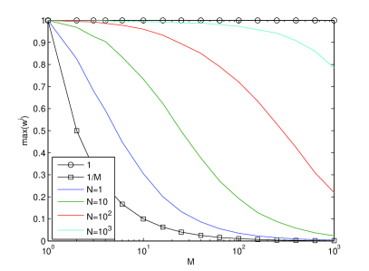
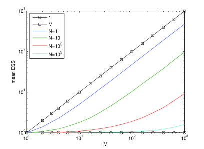
For this model, we have analyzed the behavior of the maximum normalized importance weight $\max w^{(i)}$ and the effective sample size $M^{eff}$, when the number of observations $N$ increases. We consider a number of observations $N$ varying from 1 to $10^{3}$, and a number of samples $M$ also varying from 1 to $10^{3}$. For each pair of $N$ and $M$ we have performed $P=10^{3}$ simulation runs, generating an independent vector of observations y and an independent set of samples $\Theta^{M}$ in each run.

In Figure 1 (left) the maximum importance weight averaged over $P$ simulation runs is represented as a function of the number of samples $M$ and the number of observations $N$. The curves representing the extreme cases $\max_{i}w^{(i)}=1/M$ (uniform weights) and $\max_{i}w^{(i)}=1$ (degeneracy) are also plotted on the graph. It can be observed that, as the number of observations, $N$, increases, and considering a fixed number of samples $M$, the maximum importance weight moves apart from the optimal value $1/M$ and approaches degeneracy, where $\max_{i}w^{(i)}=1$. This indicates that an increase in the number of observations causes an increase in the fluctuations of the importance weights.

On the other hand, in Figure 1 (right) the average ESS is also represented for several values of $M$ and $N$. The cases when the ESS is maximum, $M^{eff}=M$, and minimum, $M^{eff}=1$, are plotted on the graph for reference. It can be observed that, as the number of observations $N$ increases, the ESS is smaller for the same value of $M$. Actually, while the ESS always grows with $M$, its slope becomes very small for large values of $N$. For example, with $N=1000$ observations and $M=1000$ samples, we only obtain 1.5 effective samples on average.

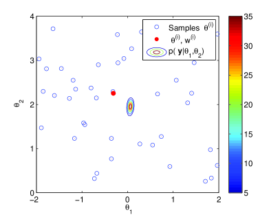
In Figure 2 an example of degeneracy in this simple setup is shown. A set of $M=200$ samples has been drawn from the prior pdf and standard importance weights have been computed from the likelihood. A subset of these samples is depicted in figure 2 together with the associated weights. The likelihood function evaluated in the same region is depicted with contour lines and it presents high variations due to the high number of observations. It can be observed that only a small fraction of the sample set is close to the region where the likelihood is significant. As a result, one sample has a weight close to 1 and the rest of them have negligible weights.

Figure 2: Subset of $M=200$ samples $\boldsymbol{\theta}^{(i)}$ drawn form the prior $p(\boldsymbol{\theta})$ (blue circles) and the associated standard importance weights (red circles with size proportional to the weight $w^{(i)}$). The likelihood function $p(\textbf{y}|\boldsymbol{\theta})$ is depicted with contour lines.

7.3 Comparison of algorithms

In this section we compare, by way of computer simulations, the performance of the two proposed schemes (NPMC with tempering and with clipping, see Section 5) and the standard PMC algorithm when applied to the Gaussian mixture model. For convenience, we reproduce in Table 4 the original PMC scheme proposed in Cappe04 .

Table 4: Standard PMC algorithm of Cappe04 .

Initialization ($\ell=0$):

1. Consider a set of $p$ scales (variances) $v_{j}$ and an initial number $r_{j}=m$ of samples per scale, $j=1,\ldots,p$.

2. For $i=1,\ldots,M=pm$, draw $\left\{\boldsymbol{\theta}_{0}^{(i)}\right\}$ from $q_{0}(\boldsymbol{\theta})=p(\boldsymbol{\theta})$.

Iteration ($\ell=1,\ldots,L$):

1. For $j=1,\ldots,p$

   • generate a sample $\left\{\boldsymbol{\theta}_{\ell}^{(i)}\right\}$ of size $r_{j}$ from

     $$q_{\ell}\left(\boldsymbol{\theta}\right)=\mathcal{N}\left(\boldsymbol{\theta}_{\ell}^{(i)};\boldsymbol{\theta}_{\ell-1}^{(i)},v_{j}\textbf{I}_{K}\right),\quad i=1,\ldots,M,$$

   • compute the normalized weights

     $$w_{\ell}^{(i)}\propto\frac{p\left(\textbf{y}|\boldsymbol{\theta}_{\ell}^{(i)}\right)p\left(\boldsymbol{\theta}_{\ell}^{(i)}\right)}{q_{\ell}\left(\boldsymbol{\theta}_{\ell}^{(i)}\right)}.$$

2. Resample with replacement the set $\left\{\boldsymbol{\theta}_{\ell}^{(i)}\right\}_{i=1}^{M}$ according to the weights $w_{\ell}^{(i)}$ to obtain $\left\{\tilde{\boldsymbol{\theta}}_{\ell}^{(i)}\right\}_{i=1}^{M}$.

3. For $j=1,\ldots,p$ update $r_{j}$ as the number of elements generated with variance $v_{j}$ which have been resampled.

In order to asses the merit of an unweighted sample set $\{\tilde{\theta}_{k}^{(i)}\}_{i=1}^{M}$ for the estimation of a scalar variable of interest $\theta_{k}$, we evaluate the mean square error (MSE)

$$MSE_{k}=\frac{1}{M}\sum_{i=1}^{M}\left(\tilde{\theta}_{k}^{(i)}-\theta_{k}\right)^{2},$$

where $M$ is the sample size and $k\in\{1,...,K\}$.

The parameters common to all the algorithms have been set to $M=200$ samples per iteration and $L=20$ iterations. We have performed $P=10^{3}$ independent simulation runs, with an independent random vector of observations y at each run. The standard PMC algorithm and the proposed NPMC technique, both with tempering and clipping (labeled NPMC temp and NPMC clip, respectively, in the figures) have been run with the same observation vector y and the results have been compared in terms of the NESS and the MSE.

	mean NESS	std NESS	mean $MSE_{1}$	mean $MSE_{2}$	std $MSE_{1}$	std $MSE_{2}$
PMC	0.131	0.063	0.037	$4.5\times 10^{-3}$	$135.4\times 10^{-3}$	$591.1\times 10^{-6}$
NPMC temp	0.937	0.059	0.019	$3.3\times 10^{-3}$	$0.19\times 10^{-3}$	$5.71\times 10^{-6}$
NPMC clip	0.937	0.060	0.019	$3.3\times 10^{-3}$	$0.19\times 10^{-3}$	$5.68\times 10^{-6}$
True posterior	-	-	0.019	$3.3\times 10^{-3}$	$0.18\times 10^{-3}$	$5.53\times 10^{-6}$

Table 5: Mean and standard deviation of the NESS, MSE of $\theta_{1}$ and MSE of $\theta_{2}$ for PMC, NPMC-temp and NPMC-clip.

The specific parameters of the plain PMC algorithm have been selected as suggested in Cappe04 ($p=5$ scales, $\textbf{v}=[5,2,0.1,0.05,0.01]^{\top}$, $m=40$ samples per scale). A minimum of 1% of $M$ of samples per scale has been kept as a baseline.

In the NPMC algorithm with tempering, the sequence of parameters $\gamma_{\ell}$, has been obtained from the sigmoid function of the iteration index, namely,

$$\gamma_{\ell}=\frac{1}{1+e^{-(\ell-5)}},\quad\ell=1,\ldots,L.$$

With this choice of nonlinearity, the transformation of the weights is practically eliminated after 10 iterations and the algorithm performs standard IS.

The NPMC algorithm with clipping has been simulated in its modified version, i.e., with the nonlinear transformation removed when the ESS reaches a value of $M_{min}^{eff}=100$. In this problem, the simulations show that this occurs on average at the iteration $\ell=5$. The parameter $M_{T}$ has been set to $M_{T}=M/4=50$ samples.

Figure 3: Evolution of the NESS for the standard PMC, NPMC with tempering and NPMC with clipping.

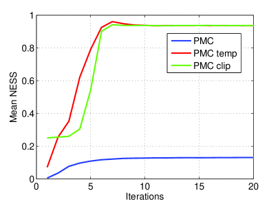
In Figures 3 and 4 numerical results comparing the performance of the three algorithms (PMC, NPMC with tempering and NPMC with clipping) are displayed. In Figure 3 the evolution of the average NESS along the iterations is depicted. It can be observed that the original PMC scheme presents a low NESS, converging to a value of 0.131. As a consequence of the degeneracy problem, the estimates of the variables of interest obtained from this reduced set of representative samples are often poor, presenting its variance large fluctuations along the iterations. Since the proposal density is updated based on the set of samples at the previous iteration, the update procedure also suffers from the lack of useful samples, leading to a very “noisy” convergence of the algorithm. On the contrary, the two NPMC schemes provide a smooth convergence of the NESS to a value of 0.937 in about 10 iterations.

Figure 4: Evolution of the MSE of parameters $\theta_{1}$ (left) and $\theta_{2}$ (right) for the different PMC schemes.

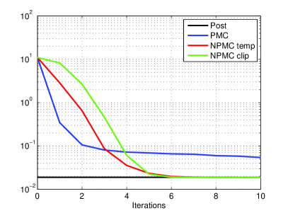
The degeneracy problem is most critical at the first iterations of the PMC, when the proposal pdf does not usually fit the target density. It is thus extremely hard to obtain a set of representative samples (with non-negligible importance weights), which allow for a consistent and robust proposal update. In Figure 3, the starting value of the NESS corresponds to $M_{T}/M=0.25$ for NPMC with clipping, 0.08 for NPMC with tempering and around 0.01 for the standard PMC algorithm.

The mean and standard deviation of the NESS at the last iteration are represented in Table 5 for all three algorithms. It can be checked that they present similar standard deviations, while the standard PMC presents a considerably lower mean NESS than the proposed methods.

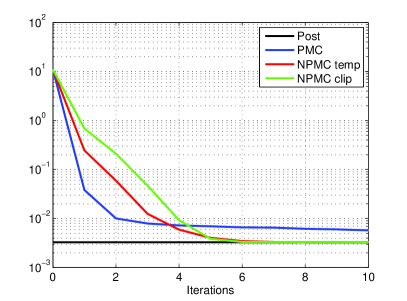
In Figure 4 the evolution along the iterations of the MSE for $\theta_{1}$ (left) and $\theta_{2}$ (right) is represented for the three algorithms. The minimum MSE of each parameter, which has been numerically approximated from the posterior pdf $p(\boldsymbol{\theta}|\textbf{y})$, is also shown for reference. Again, it can be observed that the proposed NPMC schemes converge smoothly, reaching the minimum MSE in a low number of iterations ($\ell=6$). On the other side, the original PMC does not reach the minimum MSE with the given number of samples $M=200$.

However, the most outstanding difference in the performance of the three algorithms is the extremely high variance of the MSE of the original PMC scheme. Again due to degeneracy, this algorithm presents a highly varying performance along the iterations and the simulation runs. On the contrary, the proposed schemes reach the minimum MSE, both in average and in standard deviation. The final mean values, as well as the standard deviation of the MSE for $\theta_{1}$ and $\theta_{2}$ are also shown in Table 5.

Moreover, the original PMC scheme hardly presents any adaptation along most of the iterations and it allows for no parameterization of the convergence speed. It reaches the final solution at the second iteration, which is hardly improved for the rest of the simulation. This behavior is not desirable in an iterative method, and it suggests that the adaptation is not performed in a appropriate way. On the contrary, the convergence speed of the NPMC method with clipping may be adjusted by jointly selecting the parameters $M$ and $M_{T}$, and that of NPMC with tempering, by modifying the sequence $\gamma_{\ell}$.

8 Example 2: A stochastic kinetic model

In this section, the proposed nonlinear PMC method is applied to the problem of estimating the hidden parameters of a simple stochastic kinetic model (SKM), known as the predator-prey model. A SKM is a multivariate continuous-time jump process modeling the interactions among molecules, or species, that take place in chemical reaction networks of biochemical and cellular systems Wilkinson06 ; Boys08 .

Several MCMC schemes have been recently proposed to address the problem of estimating the rate parameters in SKMs, Boys08 , Wilkinson11 , Milner06 , Golightly2011 . In Milner06 the authors propose an approximation of the likelihood based on the moment closure approximation of the underlying stochastic process. In Golightly2011 a likelihood-free particle MCMC scheme is applied to this problem. A recently proposed work addressing this kind of problems is Baragatti11 , where several MCMC schemes are proposed to address likelihood-free scenarios.

We propose an alternative approach based on the NPMC method. In particular, we introduce a modification of the generic NPMC algorithm which computes an approximation of the likelihood via a particle filter. The proposed method is exact in the sense that it simulates from the stochastic process in the model without further approximations.

8.1 Predator-prey model

The Lotka-Volterra, or predator-prey, model is a simple SKM that describes the time evolution of two species $x_{1}$ (prey) and $x_{2}$ (predator), by means of $K=3$ reaction equations: Boys08 ; Volterra26

$$\begin{array}[]{cl}x_{1}\stackrel{{\scriptstyle\theta_{1}}}{{\longrightarrow}}2x_{1}&\textrm{prey reproduction}\\ x_{1}+x_{2}\stackrel{{\scriptstyle\theta_{2}}}{{\longrightarrow}}2x_{2}&\textrm{predator reproduction}\\ x_{2}\stackrel{{\scriptstyle\theta_{3}}}{{\longrightarrow}}\emptyset&\textrm{predator death}\end{array}$$

The $k$-th reaction takes place stochastically according to its instantaneous rate $a_{k}(t)=\theta_{k}g_{k}\left(\textbf{x}(t)\right)$, where $\theta_{k}>0$ is the constant (yet random) rate parameter and $g_{k}(\cdot)$ is a continuous function of the current state of the system $\textbf{x}(t)=[x_{1}(t),x_{2}(t)]^{\top}$. We denote by $x_{1}(t),x_{2}(t)$ the nonnegative, integer population of each species at continuous time $t$. In this simple example, the instantaneous rates are of the form

$$a_{1}(t)=\theta_{1}x_{1}(t),\;a_{2}(t)=\theta_{2}x_{1}(t)x_{2}(t),\;a_{3}(t)=\theta_{3}x_{2}(t).$$

The waiting time to the next reaction is exponentially distributed with parameter $a_{0}(t)=\sum_{k=1}^{K}a_{k}(t)$, and the probability of each reaction type is given by $a_{k}(t)/a_{0}(t)$. We denote by x the vector containing the population of each species at the occurrence time of each reaction in a time interval $t\in[0,T]$, i.e.,

$$\textbf{x}=[\textbf{x}^{\top}(t_{1}),\textbf{x}^{\top}(t_{2}),\ldots,\textbf{x}^{\top}(t_{R})]^{\top},$$

where $R$ is the total number of reactions and $t_{i}\in[0,T]$, $i=1,...,R$, are the time instants at which the reactions occur. Assuming that the entire vector x is observed, the likelihood function for the rate parameter vector $\boldsymbol{\theta}=[\theta_{1},\ldots,\theta_{K}]^{\top}$ can be computed analytically Wilkinson06 ,

$$p(\textbf{x}|\boldsymbol{\theta})=\prod_{k=1}^{K}p(\textbf{x}|\theta_{k})=\prod_{k=1}^{K}\theta_{k}^{r_{k}}\exp\left\{-\theta_{k}\int_{0}^{T}g_{k}\left(\textbf{x}(t)\right)dt\right\},$$ (12)

where $r_{k}$ is the total number of reactions of type $k$ occurred in the time interval $[0,T]$.

The structure of the likelihood function in (12) allows the selection of a conjugate prior distribution for the rate parameters in the form of independent Gamma components, i.e.,

$$p(\boldsymbol{\theta})=\prod_{k=1}^{K}p(\theta_{k})=\prod_{k=1}^{K}\mathcal{G}(\theta_{k};\,a_{k},b_{k}),$$ (13)

where $a_{k},b_{k}>0$ are the scale and shape parameters of each component, respectively. Thus, the posterior distribution $p(\boldsymbol{\theta}|\textbf{x})=\prod_{k=1}^{K}p(\theta_{k}|\textbf{x})$ may be also factorized into a set of independent Gamma components

$$p(\theta_{k}|\textbf{x})=\mathcal{G}\left(\theta_{k};\;a_{k}+r_{k},b_{k}+\int_{0}^{T}g_{k}\left(\textbf{x}(t)\right)dt\right).$$

Therefore, in the complete-data scenario (in which x is observed), exact inference may be done for each rate constant $\theta_{k}$ separately. However, making inference for complex, high-dimensional and discretely observed SKMs (where x is not fully available) is a challenging problem Boys08 .

Exact stochastic simulation of generic SKMs, and predator-prey models in particular, can be carried out by the Gillespie algorithm Gillespie77 . This procedure allows to draw samples from the prior pdf of the populations, $p(\textbf{x}|\boldsymbol{\theta})$, for arbitrary SKMs.

Although in this work we restrict ourselves to the predator-prey model, which is a simple but representative example of SKM, the proposed algorithm may be equally applied to the estimation of parameters of SKMs of higher complexity.

8.2 NPMC algorithm for SKMs

We assume that a set of $N$ noisy observations of the populations of both species are collected at regular time intervals of length $\Delta$, that is, $\textbf{y}_{n}=\textbf{x}_{n}+\textbf{u}_{n},\;n=1,\ldots,N$, where $\textbf{x}_{n}=[x_{1}(n\Delta),x_{2}(n\Delta)]^{\top}$ and $\textbf{u}_{n}$ is a Gaussian noise component with zero mean vector and covariance matrix $\sigma^{2}\textbf{I}$. We denote the complete vector of observations as $\textbf{y}=[\textbf{y}_{1}^{\top},\ldots,\textbf{y}_{N}^{\top}]^{\top}$ with dimension $2N\times 1$. Thus, the likelihood of the populations x is given by

$$p\left(\textbf{y}|\textbf{x}\right)=\prod_{n=1}^{N}\mathcal{N}\left(\textbf{y}_{n};\,\textbf{x}_{n},\sigma^{2}\textbf{I}\right).$$

The goal is to approximate the posterior distribution, with density $p(\boldsymbol{\theta}|\textbf{y})\propto p(\textbf{y}|\boldsymbol{\theta})p(\boldsymbol{\theta})$, given the prior pdf $p(\boldsymbol{\theta})$ and the likelihood $p(\textbf{y}|\boldsymbol{\theta})$, using the NPMC method.

In this particular problem, the observations y are related to the variables $\boldsymbol{\theta}$ through the random vector x. Indeed, the likelihood of ${\boldsymbol{\theta}}$ has the form

$$p(\textbf{y}|\boldsymbol{\theta})=\int p(\textbf{y}|\textbf{x})p(\textbf{x}|\boldsymbol{\theta})d\textbf{x}=E_{p(\textbf{x}|\boldsymbol{\theta})}\left[p(\textbf{y}|\textbf{x})\right],$$ (14)

where $E_{p(\textbf{x}|\boldsymbol{\theta})}[\cdot]$ denotes expectation with respect to the pdf in the subscript, and $p(\textbf{y}|\textbf{x},\boldsymbol{\theta})=p(\textbf{y}|\textbf{x})$, since the observations are independent of the parameters $\boldsymbol{\theta}$ given the population vector x. As a consequence, the likelihood of the parameters cannot be evaluated exactly. A set of likelihood-free techniques have been recently proposed to tackle this kind of problems, which avoid the need to evaluate the likelihood function Baragatti11 . However, in this work we follow a different approach which consists in computing an approximation of the likelihood of $p(\textbf{y}|\boldsymbol{\theta})$.

In principle, it is possible to approximate the integral in (14) as an average of the likelihoods $p(\textbf{y}|\textbf{x}^{(i)})$ of a set $\{\textbf{x}^{(i)}\}_{i=1}^{I}$ of exact Monte Carlo samples from the density $p(\textbf{x}|\boldsymbol{\theta})$, drawn using the Gillespie algorithm, that is,

$$p(\textbf{y}|\boldsymbol{\theta})\approx\frac{1}{I}\sum_{i=1}^{I}p\left(\textbf{y}\left|\right.\textbf{x}^{(i)}\right).$$

This approach, however, is computationally intractable, because it demands drawing a huge number of samples $I$ to obtain a useful approximation of the likelihood $p(\textbf{y}|\boldsymbol{\theta})$, since the probability of generating a trajectory of populations $\textbf{x}^{(i)}$ similar to the observations is extremely low.

To overcome this difficulty, we propose a simple approach based on using a standard particle filter. An approximation for the likelihood of the parameters $p(\textbf{y}\left|\right.\boldsymbol{\theta}^{(i)})$ may be recursively obtained based on the particle filter approximation of the posterior of the populations $p(\textbf{x}\left|\right.\textbf{y},\boldsymbol{\theta}^{(i)})$. Indeed, the likelihood of a sample $\boldsymbol{\theta}^{(i)}$ can be recursively factorized as

$$p\left(\textbf{y}\left|\right.\boldsymbol{\theta}^{(i)}\right)=\prod_{n=1}^{N}p\left(\textbf{y}_{n}\left|\right.\textbf{y}_{1:n-1},\boldsymbol{\theta}^{(i)}\right)$$

where each of the terms in the product (with fixed $\boldsymbol{\theta}={\boldsymbol{\theta}}^{(i)}$) can be approximated via particle filtering (see, e.g., Djuric10 or Maiz12 ).

The NPMC method for this application is exact in the sense that it uses exact samples $\textbf{x}^{(i)}$ from the stochastic model generated via the Gillespie algorithm, and does not perform any approximation of the stochastic process. Alternative approaches have been proposed which employ a diffusion approximation. However, this approximation has not shown to introduce any improvement to our algorithm.

To summarize, the standard importance weights for this application have the form

$$w_{\ell}^{(i)*}\propto\frac{\hat{p}\left(\textbf{y}\left|\right.\boldsymbol{\theta}_{\ell}^{(i)}\right)p\left(\boldsymbol{\theta}_{\ell}^{(i)}\right)}{q_{\ell}\left(\boldsymbol{\theta}_{\ell}^{(i)}\right)},$$

where the likelihood $\hat{p}(\textbf{y}|\boldsymbol{\theta}_{\ell}^{(i)})$ is approximated using a particle filter. The prior is a product of $K$ independent Gamma components as in Eq. (13) and the proposal is a multivariate normal pdf, as shown in Table 2.

Let us finally remark that, while in this work we have focused on the complete-observation scenario, the proposed method is also valid in the partially observed case, when only a subset of the species can be observed.

8.3 Computer simulation results

We have applied the NPMC algorithm to the problem of estimating the posterior pdf of the constant rate parameters vector $\boldsymbol{\theta}$ in a simple predator-prey model. The true vector of parameter rates which we aim to estimate has been set to

$$\boldsymbol{\theta}=[0.5,0.0025,0.3]^{\top}.$$

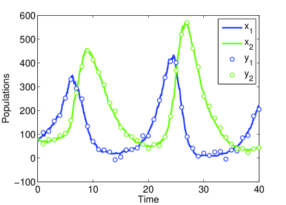
A realization of the populations x has been generated from the prior distribution $p(\textbf{x}|\boldsymbol{\theta})$ with initial populations $\textbf{x}(0)=[71,79]^{\top}$, and a total length of $T=40$. The observation vector y has been generated with an observation period $\Delta=1$ and a Gaussian noise variance $\sigma^{2}=100$.

Figure 5 depicts the time evolution of the true populations of both species x, and the corresponding discrete-time noisy observations y. The autoregulatory behavior of the model can be clearly observed on the graph.

Figure 5: Real populations (x) and discrete-time noisy observations (y) in a predator-prey model.

The parameters of the prior Gamma distribution $p(\boldsymbol{\theta})$ have been chosen such that the corresponding mean matches the real value of $\boldsymbol{\theta}$ and the marginal standard deviations are $[1.25,0.0065,0.77]^{\top}$. These priors cover an order of magnitude either side of the true value, which represents a vague prior knowledge.

The target density for the NPMC algorithm is the posterior pdf, $\pi(\boldsymbol{\theta})=p(\boldsymbol{\theta}|\textbf{y})$. Despite the low dimension of this problem ($K=3$), the importance weights of the PMC scheme present severe degeneracy, partially due to the likelihood approximation. In the simulations, we have observed that the importance weights present such degeneracy, that, for the NPMC scheme with tempering, the coefficient $\gamma_{\ell}$ must take extremely low values (about $10^{-4}$) at the first iterations in order to balance the weights and obtain a reasonable number of effective samples. Besides, the sequence $\gamma_{\ell}$ is hard to design a priori, and it does not guarantee that the resulting sample set leads to accurate estimates. For that reasons, in this example we have restricted our attention to the hard clipping technique, which does not require the fitting of any parameters and guarantees a baseline ESS. Recall that the NPMC scheme with hard clipping only requires the selection of a unique parameter $M_{T}$, which allows to adjust the convergence performance of the algorithm, and does not require a precise fitting. In this example, we have chosen $M_{T}=M/5$, with a total number of samples $M=500$ and $L=10$ iterations.

In order to be able to compare the MSE of parameters $\theta_{k}$, $k=1,2,3$, that take very different values, we additionally define normalized MSEs (NMSE) as

$$NMSE_{k}=\frac{1}{M}\sum_{i=1}^{M}\left(\frac{\tilde{\theta}_{k}^{(i)}-\theta_{k}}{\theta_{k}}\right)^{2}=\frac{MSE_{k}}{\theta_{k}^{2}},\quad k=1,2,3,$$

and a global error figure as the average NMSE, namely

$$NMSE=\frac{1}{K}\sum_{k=1}^{K}NMSE_{k}.$$

We have carried out two different experiments. In both experiments we have performed $P=100$ independent simulation runs, with the same true parameters $\boldsymbol{\theta}$ and initial populations $\textbf{x}(0)$, but different (independent) population and observations vectors x and y in each run.

In the first experiment we considered the same number of samples $M=500$ in all the simulation runs of the NPMC algorithm and computed the NESS and the NMSE along the iterations. We observed that a 70% of the simulation runs converged to yield accurate estimates (with low NMSE), while in a 30% of the cases, the algorithm produced biased estimates, with considerably higher NMSE and low final NESS (below a 0.3).

Figure 6: Left: Average value of $\log_{10}(\mbox{NMSE})$ versus the NESS after the last iteration ($L=10$) for each simulation run, with $M=500$ samples. The histogram of each variable is also represented. Right: Average value of $\log_{10}(\mbox{NMSE})$ versus the NESS after the last iteration ($L=10$) for each simulation run, with $M=500$ for 70% of the simulation runs, $M=1000$ for the 28% of the simulation runs and $M=2000$ for 8% of the simulation runs.

Figure 7: Left: Evolution of the mean NESS, before and after clipping. The NESS before clipping (computed for the standard weights) is labeled NESS orig. Right: Evolution of the mean MSE. The lower bound is obtained from the optimal posterior $p(\boldsymbol{\theta}|\textbf{x})$ (labeled Opt post in the figure).

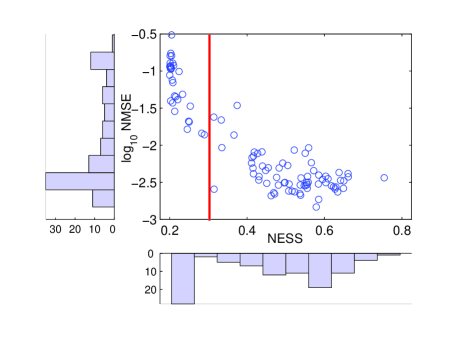
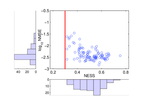
In Figure 6 (left) the final values of the logarithm of the NMSE versus the NESS obtained for each simulation run are depicted, together with the histograms of both the $\log_{10}(\mbox{NMSE})$ and the NESS. This plot reveals how low NESS values correspond to high NMSE, and viceversa. This empirical relationship is relevant because allows to detect, in practice, whether the algorithm has converged properly or not.

The second experiment consisted in repeating the simulation of the algorithm in those cases which did not yield accurate estimates with $M=500$ samples, but increasing the number of samples to $M=1000$. For this new experiment, we considered that the algorithm had converged when the final NESS was greater than 0.3. Out of the repeated simulations, 8 cases still did not converge and the simulations were repeated with $M=2000$. Finally, all the simulation runs obtained a final NESS$>0.3$ with a number of particles $M=500$ for the 70% of the cases, $M=1000$ for the 22% of the cases and $M=2000$ for the 8% of the cases.

In Figure 6 (right) the final values of $\log_{10}(\mbox{NMSE})$ versus the NESS are plotted after repeating the simulations with $M=1000$ (22% of the runs) and $M=2000$ (8% of the runs). It can be observed that the points with high NMSE are removed and that most points concentrate in the region of high NESS and low NMSE. Also the histograms of NMSE and NESS show how their mean values significantly improve.

	MSE $\theta_{1}$	MSE $\theta_{2}$	MSE $\theta_{3}$	NMSE $\theta_{1}$	NMSE $\theta_{2}$	NMSE $\theta_{3}$	mean NMSE
Prior	$1.56$	$4.42\times 10^{-5}$	$0.5929$	$6.25$	$6.76$	6.588	6.533
NPMC clip (1)	$9.7\times 10^{-3}$	$53.0\times 10^{-9}$	$36.8\times 10^{-4}$	0.03878	0.008484	0.04089	0.02938
NPMC clip (2)	$1.4\times 10^{-3}$	$23.46\times 10^{-9}$	$6.38\times 10^{-4}$	0.005618	0.003754	0.007092	0.005488
Optimal posterior	$0.26\times 10^{-3}$	$5.53\times 10^{-9}$	$0.881\times 10^{-4}$	$0.00103$	$0.0008862$	0.0009796	0.0009654

Table 6: Final mean MSE and NMSE for the parameters $\theta_{1}$, $\theta_{2}$ and $\theta_{3}$ in experiments 1 and 2. The prior and optimal posterior values are included for comparison.

Figure 8: Example of pdfs of interest of a particular simulation run with final NMSE of 0.0053 (close to the average NMSE): marginal priors $p(\theta_{k})$, optimal posteriors $p(\theta_{k}|\textbf{x})$, estimated posteriors $\hat{p}(\theta_{k}|\textbf{y})$ and true values $\theta_{k}$ for $k=1$ (left), $k=2$ (central) and $k=3$ (right).

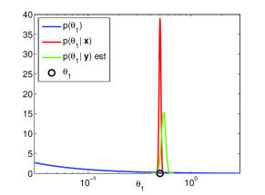
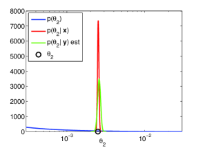
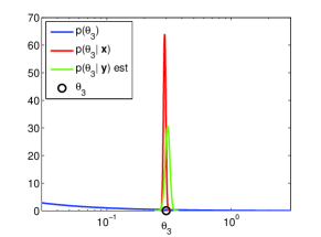
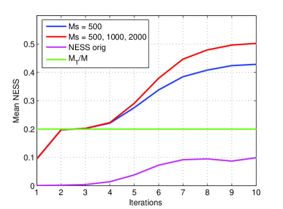
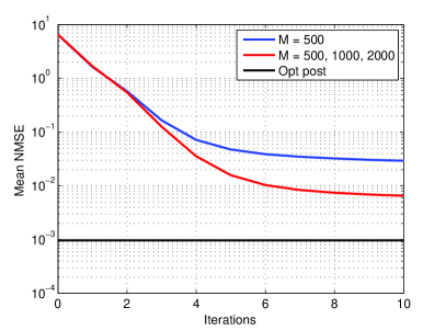
Figure 7 shows the evolution of the mean NESS and NMSE along the iterations in both experiments. In solid blue lines, the results regarding the first experiment are plotted ($M=500$ for all simulation runs). In solid red lines, the results of the second experiment are represented ($M=500$, $M=1000$ and $M=2000$).

In Figure 7 (left) the evolution of the NESS, $M_{\ell}^{neff}$, after the clipping procedure in both experiments is represented. In both cases it starts from an initial value of $M_{T}/M$ and reaches a final value of about 0.43 in the first case and 0.5 in the second case. Also the NESS before clipping (i.e., for the standard weights) is represented in this graph, which takes significantly lower values, but presents a significant increase after the first iterations. In this example, the clipping procedure has been performed along all the iterations because of the severe degeneracy of the weights. This is probably due to the approximation in the computation of the likelihood $p(\textbf{y}|\boldsymbol{\theta})$, which leads to additional fluctuations in the values of the importance weights, increasing the effects of degeneracy.

Figure 7 (right) shows the evolution of the NMSE along the iterations, as well as the corresponding lower bound given by the optimal marginal posterior with complete data, $p(\theta_{k}|\textbf{x})$, in both experiments. The starting value at $\ell=0$ corresponds to the vague knowledge described by the prior distribution. It can be seen that the NMSE of the NPMC algorithms with clipping smoothly decreases until a final value close to the lower bound, in a low number of iterations.

Table 6 summarizes the obtained results in terms of MSE and NMSE for each parameter $\theta_{k}$ for both experiments. It can be observed that the prior distribution provides vague knowledge of the variables of interest, with a high MSE and NMSE. The NMSE allows to compare the error values of the three parameters, even when $\theta_{2}$ has a very low value with respect to $\theta_{1}$ and $\theta_{3}$.

In the first experiment we obtain a remarkable reduction in MSE and NMSE with respect to the prior. However, increasing the number of samples in a fraction of cases allows to further reduce the estimation error. The MSE and NMSE of the optimal marginal posteriors are also shown for comparison. Note, however, that this is an unreachable performance bound, since it is obtained when the whole vector x is observed.

In order to illustrate the quality of the obtained approximations, Figure 8 depicts the final estimate of the marginal posteriors $p(\theta_{k}|\textbf{y})$, together with the corresponding prior $p(\theta_{k})$ and the optimal posterior in the complete-data scenario $p(\theta_{k}|\textbf{x})$. It can be observed that the algorithm provides a good approximation of the

9 Conclusion

We have addressed the problem of approximating posterior probability distributions by means of random samples. A recently proposed approach to tackle this problem is the population Monte Carlo method, that consists in iteratively approximating a target distribution via an importance sampling scheme. The main limitation of this algorithm is that is presents severe degeneracy of the importance weights as the dimension of the model, $K$, and/or the number of observations, $N$, increase. This leads to a highly varying number of effective samples and inaccurate estimates, unless the number of samples is extremely high (which makes the method computationally prohibitive).

We propose to apply a simple procedure in order to guarantee a prescribed ESS and a smooth and robust convergence. It consists in applying nonlinear transformations to the standard importance weights in order to reduce their fluctuations and thus avoid degeneracy. In order to illustrate the application of the proposed technique, we have applied it to two examples of different complexity. The first example is a simple GMM, which allows to get insight of the performance of the standard PMC scheme, the degeneracy problem and the behavior of the proposed algorithm.

We have tackled the problem of estimating the set of constant (and random) rate parameters of a stochastic kinetic model. Even for the relatively simple predator-prey model that we have studied, this is significantly more complex than the GMM example. We have shown extensive simulation results that show how the proposed NPMC scheme can greatly improve the performance of the standard method.

The convergence of standard PMC algorithms is often justified by the asymptotic convergence of IS (with respect to the number of samples). The NPMC scheme modifies the importance weights and, hence, the standard theory of IS cannot be applied directly. To address this difficulty, we have analyzed the convergence of the approximations of integrals computed using transformed importance weights and proved that they converge a.s., similar to the results available for standard IS.

Appendix A Proof of Lemma 1

As a first step, we seek a tractable upper bound for the difference

$$\left|(f,\bar{\pi}^{M})-(f,\check{\pi}^{M})\right|=\left|\sum_{i=1}^{M}f({\boldsymbol{\theta}}^{(i)})\left(\bar{w}^{(i)}-\check{w}^{(i)}\right)\right|,$$ (15)

where

$$\bar{w}^{(i)} = \frac{(\varphi^{M}\circ g)({\boldsymbol{\theta}}^{(i)})}{\sum_{j=1}^{M}(\varphi^{M}\circ g)({\boldsymbol{\theta}}^{(j)})}\quad\mbox{and}$$ (16)

$$\check{w}^{(i)} = \frac{(\varphi^{M}\circ g)({\boldsymbol{\theta}}^{(i)})}{\sum_{j=1}^{M}g({\boldsymbol{\theta}}^{(j)})},$$ (17)

and $(\varphi^{M}\circ g)(\boldsymbol{\theta})=\varphi^{M}(g(\boldsymbol{\theta}))$ denotes the composition of the functions $\varphi^{M}$ and g. Moreover, the constants in the denominators of the weights can be written as integrals with respect to the random measure

$$q^{M}(d\boldsymbol{\theta})=\frac{1}{M}\sum_{j=1}^{M}\delta_{{\boldsymbol{\theta}}^{(j)}}(d\boldsymbol{\theta}),$$ (18)

namely,

$$\sum_{j=1}^{M}(\varphi^{M}\circ g)({\boldsymbol{\theta}}^{(j)})=M(\varphi^{M}\circ g,q^{M})$$ (19)

and

$$\sum_{j=1}^{M}g({\boldsymbol{\theta}}^{(j)})=M(g,q^{M}).$$ (20)

Substituting (16), (17), (19) and (20), into (15) yields, after straightforward manipulations,

$$\left|(f,\bar{\pi}^{M})-(f,\check{\pi}^{M})\right|=\left|\frac{1}{M}\sum_{i=1}^{M}f({\boldsymbol{\theta}}^{(i)})(\varphi^{M}\circ g)({\boldsymbol{\theta}}^{(i)})\frac{(g,q^{M})-(\varphi^{M}\circ g,q^{M})}{(\varphi^{M}\circ g,q^{M})(g,q^{M})}\right|.$$ (21)

A useful upper bound for the difference of integrals follows quite easily from (21). In particular, note that $|f({\boldsymbol{\theta}}^{(i)})(\varphi^{M}\circ g)|\leq\|f\|_{\infty}\|g\|_{\infty}$, since $f,g\in B(\mathbb{R}^{K})$ and $\varphi^{M}\circ g\leq g$, while the latter inequality also implies that $(\varphi^{M}\circ g,q^{M})(g,q^{M})\geq(\varphi^{M}\circ g,q^{M})^{2}$. Also note that, from the definition of $\varphi^{M}$,

$$|(g,q^{M})-(\varphi^{M}\circ g,q^{M})| \leq \frac{1}{M}\sum_{k=1}^{M_{T}}|g({\boldsymbol{\theta}}^{(i_{k})})-(\varphi^{M}\circ g)({\boldsymbol{\theta}}^{(i_{k})})|$$ (22)

$$\leq \frac{2M_{T}\|g\|_{\infty}}{M}.$$

As a result, we obtain

$$\left|(f,\bar{\pi}^{M})-(f,\check{\pi}^{M})\right|\leq\frac{2\|f\|_{\infty}\|g\|_{\infty}^{2}M_{T}}{M(\varphi^{M}\circ g,q^{M})^{2}}.$$ (23)

Let $c_{1}>0$ be some arbitrary real constant. From (23),

$$\mathbb{P}\left\{\left|(f,\bar{\pi}^{M})-(f,\check{\pi}^{M})\right|\leq\frac{M_{T}}{M}c_{1}\right\}\geq\mathbb{P}\left\{\frac{2\|f\|_{\infty}\|g\|_{\infty}^{2}M_{T}}{M(\varphi^{M}\circ g,q^{M})^{2}}\leq\frac{M_{T}}{M}c_{1}\right\}.$$ (24)

If we choose

$$c_{1}=\frac{2\|f\|_{\infty}\|g\|_{\infty}^{2}}{\left(\frac{1}{a}-\frac{1}{\sqrt{2}}\right)^{2}(g,q)^{2}},$$ (25)

where $1<a<\sqrt{2}$, then substituting (25) into the right hand side of (24) yields

$$\mathbb{P}\left\{\frac{2\|f\|_{\infty}\|g\|_{\infty}^{2}M_{T}}{M(\varphi^{M}\circ g,q^{M})^{2}}\leq\frac{M_{T}}{M}c_{1}\right\} = \mathbb{P}\left\{(\varphi^{M}\circ g,q^{M})^{2}\geq\left(\frac{1}{a}-\frac{1}{\sqrt{2}}\right)^{2}(g,q)^{2}\right\}$$ (26)

$$= \mathbb{P}\left\{(\varphi^{M}\circ g,q^{M})-\frac{1}{a}(g,q)\geq-\frac{1}{\sqrt{2}}(g,q)\right\},$$

$$= \mathbb{P}\left\{M(\varphi^{M}\circ g,q^{M})-\frac{M}{a}(g,q)\geq-\frac{M}{\sqrt{2}}(g,q)\right\},$$

where the second equality holds because $\frac{1}{a}-\frac{1}{\sqrt{2}}>0$.

Next, consider the expectations $E_{q}[(\varphi^{M}\circ g,q^{M})]$ and $E_{q}[(g,q^{M})]=(g,q)$. Since, $|(\varphi^{M}\circ g,q^{M})-(g,q^{M})|\leq 2M_{T}\|g\|_{\infty}/M$ (see Eq. (22)), it follows that

$$\left|E_{q}\left[(\varphi^{M}\circ g,q^{M})\right]-E_{q}\left[(g,q^{M})\right]\right| \leq E_{q}\left[|(\varphi^{M}\circ g,q^{M})-(g,q^{M})|\right]$$

$$\leq \frac{2M_{T}\|g\|_{\infty}}{M}.$$

Therefore, since we have assumed that $\lim_{M\rightarrow\infty}\frac{M_{T}}{M}=0$ and $g>0$, there exists $M_{a}$ such that, for all $M>M_{a}$,

$$E_{q}\left[(\varphi^{M}\circ g,q^{M})\right]>\frac{1}{a}E_{q}\left[(g,q^{M})\right]=\frac{1}{a}(g,q),$$ (27)

and combining Eq. (26) with the inequality (27) we obtain that

$$\mathbb{P}\left\{\frac{2\|f\|_{\infty}\|g\|_{\infty}^{2}M_{T}}{M(\varphi^{M}\circ g,q^{M})^{2}}\leq\frac{M_{T}}{M}c_{1}\right\}\geq$$

$$\mathbb{P}\left\{M(\varphi^{M}\circ g,q^{M})-ME_{q}\left[(\varphi^{M}\circ g,q^{M})\right]\geq-\frac{M}{\sqrt{2}}(g,q)\right\}.$$ (28)

Since $M(\varphi^{M}\circ g,q^{M})=\sum_{i=1}^{M}\varphi^{M}(g({\boldsymbol{\theta}}^{(i)}))$ is the sum of $M$ independent and bounded random variables, each of them taking values within the interval $(0,\|g\|_{\infty})$, it is straightforward to apply Hoeffding’s tail inequality Hoeffding63 to obtain a lower bound on (28), namely

$$\mathbb{P}\left\{M(\varphi^{M}\circ g,q^{M})-ME_{q}\left[(\varphi^{M}\circ g,q^{M})\right]\geq-\frac{M}{\sqrt{2}}(g,q)\right\}\geq 1-\exp\left\{-\frac{(g,q)^{2}}{\|g\|_{\infty}^{2}}M.\right\}.$$ (29)

Substituting (29) back into (28), (26) and (24) yields the desired result,

$$\mathbb{P}\left\{\left|(f,\bar{\pi}^{M})-(f,\check{\pi}^{M})\right|\leq\frac{M_{T}}{M}c_{1}\right\}\geq 1-\exp\left\{-c_{1}^{\prime}M\right\},$$ (30)

with $c_{1}^{\prime}=\frac{(g,q)^{2}}{\|g\|_{\infty}^{2}}$.

Appendix B Proof of Lemma 2

The argument is similar to that of the proof of Lemma 1. Recalling Eqs. (17), (18) and (20) in Appendix A as well as the form of the standard normalized weights,

$$w^{(i)}=\frac{g({\boldsymbol{\theta}}^{(i)})}{M(g,q^{M})},$$

it is straightforward to show that

$$\left|(f,\check{\pi}^{M})-(f,\pi^{M})\right|=\frac{1}{M(g,q^{M})}\left|\sum_{k=1}^{M_{T}}f({\boldsymbol{\theta}}^{(i_{k})})\left((\varphi^{M}\circ g)({\boldsymbol{\theta}}^{(i_{k})})-g({\boldsymbol{\theta}}^{(i_{k})})\right)\right|,$$

which readily yields the upper bound

$$\left|(f,\check{\pi}^{M})-(f,\pi^{M})\right|\leq\frac{2\|f\|_{\infty}\|g\|_{\infty}M_{T}}{M(g,q^{M})}.$$ (31)

Let $c_{2}>0$ be some arbitrary real constant. From (31),

$$\mathbb{P}\left\{\left|(f,\check{\pi}^{M})-(f,\pi^{M})\right|\leq\frac{M_{T}}{M}c_{2}\right\}\geq\mathbb{P}\left\{\frac{2\|f\|_{\infty}\|g\|_{\infty}M_{T}}{M(g,q^{M})}\leq\frac{M_{T}}{M}c_{2}\right\}$$ (32)

and if we choose

$$c_{2}=\frac{2\|f\|_{\infty}\|g\|_{\infty}}{\left(1-\frac{1}{\sqrt{2}}\right)(g,q)},$$

then

$$\mathbb{P}\left\{\frac{2\|f\|_{\infty}\|g\|_{\infty}M_{T}}{M(g,q^{M})}\leq\frac{M_{T}}{M}c_{2}\right\} = \mathbb{P}\left\{(g,q^{M})\geq\left(1-\frac{1}{\sqrt{2}}\right)(g,q)\right\}$$ (33)

$$= \mathbb{P}\left\{M(g,q^{M})-M(g,q)\geq-\frac{M}{\sqrt{2}}(g,q)\right\}.$$

Since $(g,q)=E_{q}[(g,q^{M})]$ and $(g,q^{M})$ is the sum of $M$ independent, and bounded, random variables taking values within the interval $(0,\|g\|_{\infty}]$ (recall that $g>0$), we can readily apply Hoeffding’s tail inequality Hoeffding63 on Eq. (33) to obtain

$$\mathbb{P}\left\{M(g,q^{M})-M(g,q)\geq-\frac{M}{\sqrt{2}}(g,q)\right\}\geq 1-\exp\left\{-\frac{(g,q)^{2}}{\|g\|_{\infty}^{2}}M\right\}.$$ (34)

Substituting (34) back into (33) and (32) yields the desired result,

$$\mathbb{P}\left\{\left|(f,\check{\pi}^{M})-(f,\pi^{M})\right|\leq\frac{M_{T}}{M}c_{2}\right\}\geq 1-\exp\left\{-c_{2}^{\prime}M\right\},$$

where $c_{2}^{\prime}=\frac{(g,q)^{2}}{\|g\|_{\infty}^{2}}>0$.

Appendix C Proof of Lemma 3

The first part of Lemma 3 follows from the combination of Lemmas 1 and 2. We first note that, from Lemma 1,

$$\mathbb{P}\left\{\left|(f,\bar{\pi}^{M})-(f,\check{\pi}^{M})\right|>c_{1}\frac{M_{T}}{M}\right\}<\exp\{-c_{1}^{\prime}M\}$$ (35)

for sufficiently large $M$, while Lemma 2 implies

$$\mathbb{P}\left\{\left|(f,\check{\pi}^{M})-(f,\pi^{M})\right|>c_{2}\frac{M_{T}}{M}\right\}<\exp\{-c_{2}^{\prime}M\},$$ (36)

where $c_{2}=c_{2}^{\prime}=(g,q)^{2}/\|g\|_{\infty}^{2}$. Let $c=c_{1}+c_{2}$. Then, since

$$|(f,\bar{\pi}^{M})-(f,\pi^{M})|\leq|(f,\bar{\pi}^{M})-(f,\check{\pi}^{M})|+|(f,\check{\pi}^{M})-(f,\pi^{M})|,$$

we trivially obtain that

$$\mathbb{P}\left\{\left|(f,\bar{\pi}^{M})-(f,\pi^{M})\right|>c\frac{M_{T}}{M}\right\}\leq\mathbb{P}\left\{\left|(f,\bar{\pi}^{M})-(f,\check{\pi}^{M})\right|+\left|(f,\check{\pi}^{M})-(f,\pi^{M})\right|>c\frac{M_{T}}{M}\right\}.\\$$ (37)

However, if

$$\left|(f,\bar{\pi}^{M})-(f,\check{\pi}^{M})\right|+\left|(f,\check{\pi}^{M})-(f,\pi^{M})\right|>c\frac{M_{T}}{M}$$

is true, then

$$\left|(f,\bar{\pi}^{M})-(f,\check{\pi}^{M})\right|>c_{1}\frac{M_{T}}{M}\quad\mbox{or}\quad\left|(f,\check{\pi}^{M})-(f,\pi^{M})\right|>c_{2}\frac{M_{T}}{M},$$

or both jointly, are true. Therefore,

$$\mathbb{P}\left\{\left|(f,\bar{\pi}^{M})-(f,\check{\pi}^{M})\right|+\left|(f,\check{\pi}^{M})-(f,\pi^{M})\right|>c\frac{M_{T}}{M}\right\}$$

$$\leq\mathbb{P}\left\{\left|(f,\bar{\pi}^{M})-(f,\check{\pi}^{M})\right|>c_{1}\frac{M_{T}}{M}\right\}$$

$$+\mathbb{P}\left\{\left|(f,\check{\pi}^{M})-(f,\pi^{M})\right|>c_{2}\frac{M_{T}}{M}\right\}$$

$$\leq\exp\left\{-c_{1}^{\prime}M\right\}+\exp\left\{-c_{2}^{\prime}M\right\}$$

$$=2\exp\left\{-\frac{(g,q)^{2}}{\|g\|_{\infty}^{2}}M\right\},$$ (38)

for sufficiently large $M$, where the second inequality follows from (35) and (36), and the equality is due to the fact that $c_{1}^{\prime}=c_{2}^{\prime}$.

Combining (37) and (38) yields the first part of Lemma 3, with $c^{\prime}=(g,q)^{2}/\|g\|_{\infty}^{2}$.

The second part of Lemma 3 follows from a standard Borel-Cantelli argument. Indeed, let ${\mathcal{E}}_{M}$ be the event in which $\left|(f,\bar{\pi}^{M})-(f,\pi^{M})\right|>c\frac{M_{T}}{M}$ holds true. From the first part of the Lemma,

$$\mathbb{P}\left\{{\mathcal{E}}_{M}\right\}<2\exp\left\{-c^{\prime}M\right\},$$

with $c^{\prime}>0$, for sufficiently large $M$ (specifically, for all $M>M_{a}$, with $M_{a}$ as in the proof of Lemma 1). Therefore,

$$\sum_{M=1}^{\infty}\mathbb{P}\left\{{\mathcal{E}}_{M}\right\}\leq M_{a}+\sum_{M=M_{a}+1}^{\infty}\exp\left\{-c^{\prime}M\right\}<\infty,$$

because $M_{a}<\infty$ and $\sum_{M=M_{a}+1}^{\infty}\exp\left\{-c^{\prime}M\right\}<\infty$. As a consequence (see, e.g., (Williams91, , Theorem 2.7)), $\mathbb{P}\left\{\lim\sup{\mathcal{E}}_{M}\right\}=0,$ which implies that

$$\lim_{M\rightarrow\infty}|(f,\bar{\pi}^{M})-(f,\pi^{M})|=0\quad\mbox{a.s.}$$

∎

References

- [1] M. Baragatti, A. Grimaud, and D. Pommeret. Likelihood-free parallel tempering. Arxiv preprint arXiv:1108.3423, 2011.
- [2] T. Bengtsson, P. Bickel, and B. Li. Curse of dimensionaluty revisited: Collapse of particle filter in very large scale systems. Probability and statistics: Essay in honour of David A. Freedman, 2:316–334, 2008.
- [3] R. J. Boys, D. J. Wilkinson, and T. B. L. Kirkwood. Bayesian inference for a discretely observed stochastic kinetic model. Statistics and Computing, 18(2):125–135, 2008.
- [4] M.F. Bugallo, M. Hong, and P.M. Djuric. Marginalized population monte carlo. In Acoustics, Speech and Signal Processing, 2009. ICASSP 2009. IEEE International Conference on, pages 2925–2928. IEEE, 2009.
- [5] J. Míguez C. S. Maíz, E. Molanes-López and P. M. Djurić. A particle filtering scheme for processing time series corrupted by outliers. IEEE Transactions on Signal Processing, 9(60), September 2012.
- [6] O. Cappé, R. Douc, A. Guillin, J. M. Marin, and C. P. Robert. Adaptive importance sampling in general mixture classes. Statistics and Computing, 18(4):447–459, 2008.
- [7] O. Cappé, A. Guillin, J. M. Marin, and C. P. Robert. Population Monte Carlo. Computational and Graphical Statistics, 13(4):907–929, 2004.
- [8] P. M. Djurić and J. Míguez. Assessment of nonlinear dynamic models by Kolmogorov-Smirnov statistics. IEEE Transactions Signal Processing, 58(10):5069–5079, October 2010.
- [9] R. Douc, A. Guillin, J.M. Marin, and CP Robert. Minimum variance importance sampling via population monte carlo. ESAIM: Probability and Statistics, 11(1):427–447, 2007 DUDO!!
- [10] A. Doucet, S. Godsill, and C. Andrieu. On sequential Monte Carlo Sampling methods for Bayesian filtering. Statistics and Computing, 10(3):197–208, 2000.
- [11] D. T. Gillespie. Exact stochastic simulation of coupled chemical reactions. The Journal of Physical Chemistry, 81(25):2340–2361, 1977.
- [12] A. Golightly and D.J. Wilkinson. Bayesian parameter inference for stochastic biochemical network models using particle mcmc. Interface Focus 1. In press, 2011.
- [13] W. Hoeffding. Probability inequalities of sums of bounded random variables. Journal of the American Statistical Association, 58(301):13–30, March 1963.
- [14] E. Koblents and J. Míguez. A population Monte Carlo method for Bayesian inference and its application to stochastik kinetic models. In EUSIPCO, 2011.
- [15] A. Kong, J. S. Liu, and W. H. Wong. Sequential imputations and Bayesian missing data problems. Journal of the American Statistical Association, 9:278–288, 1994.
- [16] P. Milner, C.S. Gillespie, and D.J. Wilkinson. Moment closure based parameter inference of stochastic kinetic models. Statistics and Computing, pages 1–9, 2006.
- [17] M. Bugallo P. M. Djuric, B. Shen. Population Monte Carlo methodology a la Gibbs sampling. In EUSIPCO, 2011.
- [18] C. P. Robert and G. Casella. Monte Carlo Statistical Methods. Springer, 2004.
- [19] B. Shen, M.F. Bugallo, and P.M. Djuric. Multiple marginalized population monte carlo. EUSIPCO, 2010.
- [20] V. Volterra. Fluctuations in the abundance of a species considered mathematically. Nature, 118:558–560, 1926.
- [21] D. J. Wilkinson. Stochastic Modelling for Systems Biology. Chapman & Hall/CRC, Mathematical and Computational Biology Series, 2006.
- [22] D.J. Wilkinson. Parameter inference for stochastic kinetic models of bacterial gene regulation: A bayesian approach to systems biology. (with discussion), in Bayesian Statistics, 9, 2011.
- [23] D. Williams. Probability with Martingales. Cambdridge University Press, Cambridge (UK), 1991.