Slow flow in channels with porous walls

Abstract

We consider the slow flow of a viscous incompressible liquid in a channel of constant but arbitrary cross section shape, driven by non-uniform suction or injection through the porous channel walls. A similarity transformation reduces the Navier-Stokes equations to a set of coupled equations for the velocity potential in two dimensions. When the channel aspect ratio and Reynolds number are both small, the problem reduces to solving the biharmonic equation with constant forcing in two dimensions. With the relevant boundary conditions, determining the velocity field in a porous channels is thus equivalent to solving for the vertical displacement of a simply suspended thin plate under uniform load. This allows us to provide analytic solutions for flow in porous channels whose cross-section is e.g. a rectangle or an equilateral triangle, and provides a general framework for the extension of Berman flow (Journal of Applied Physics 24(9), p. 1232, 1953) to three dimensions.

I Introduction

Channel flows – liquid flows confined within a closed conduit with no free surfaces – are ubiquitous. In animals (LaBarbera, 1990) and plants (Holbrook & Zwieniecki, 2005) they serve as the building blocks of vascular systems, distributing energy to where it is needed and allowing distal parts of the organism to communicate. When constructed by humans, one of the major functions of channels is to transport liquids or gasses, e.g. water (irrigation and urban water systems) and energy (oil or natural gas) from sites of production to the consumer or industry.

In some cases, the channels have solid walls which are impermeable to the liquid flowing inside. In other cases, the channels have porous walls which allow the liquid to flow across the wall and thus modify the axial flow. Both are important. The first class of flow has been studied in great detail, and analytical solutions are known in a few, but important, cases (Batchelor, 1967). The latter class has received much less attention, although it is equally important. The effect of porous walls is especially important in the study of biological flows due to the presence of permeable cell walls (Holbrook & Zwieniecki, 2005) and in industrial filtration applications (Nielsen, 2012).

Some analytic solutions of the flow in porous walled channels are known, primarily due to a similarity technique first used in this context by Berman (1953). Berman’s method is closely related to those commonly used in boundary layer theory (Schlichting & Gersten, 2000) and allows for the solution of steady flows in geometries with symmetries which makes the problem two-dimensional. By demanding that the solution be of similarity form the Navier-Stokes equation is reduced to a single non-linear third-order differential equation for the velocity potential in one space dimension. The flow between parallel plates (Berman, 1953) and in a cylindrical (Yuan & Finkelstein, 1956) and annular tube (Berman, 1958) have been analyzed in this way. Time dependent flows, flows at high Reynolds numbers and questions of uniqueness and stability of these flows have since been address by a large number of workers, see e.g. Cox (1991).

In this paper, we extend Berman’s method to three dimensional similarity flows, and derive a set of equations for the velocity potential which are valid in channels of arbitrary cross section shape. At low Reynolds numbers, and when the channel is very long compared to its characteristic transverse dimension, the Navier-Stokes equation reduces to a single partial differential equation for a velocity potential in two space dimensions; the inhomogenous biharmonic equation with constant forcing. This equation, which is derived in Sec. 1, has been widely studied in the literature as is describes the transverse displacement of a simply suspended thin elastic plate under uniform load. In Sec. II.3 we provide analytic solutions to four cases of porous channel flows in geometries where the solution of the corresponding elastic problem is known: Flow in a cylindrical tube, between parallel plates, in a triangular channel, and in a rectangular channel.

II Flow in channels with porous walls

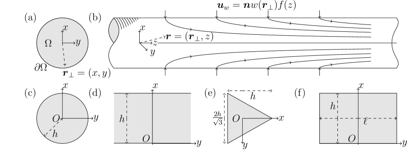
Figure 1: Flow in channels with porous walls. (a) Schematic view of the channel cross section geometry. (b) Schematic view of the axial flow geometry. See Sec. II for further details. (c-f) Sketch of geometries considered in Sec. III. In (a) and (c-f) the $z$-axis is pointing into the page.

We consider a long, straight channel parallel to the $z$-direction, and assume that it is translational invariant along this axis with an arbitrary, but constant, cross section $\Omega$ as shown in Fig. 1(a-b). The channel has length $L$, perimeter $S$, cross section area $A$, and volume $V=LA$. The coordinates in the transverse $xy$-plane are denoted $\boldsymbol{r}_{\perp}=(x,y)$, so that the full coordinates are written as $\boldsymbol{r}=\boldsymbol{r}_{\perp}+\boldsymbol{e}_{z}z$ and likewise for the gradient operator $\boldsymbol{\nabla}$, Laplace operator $\nabla^{2}$, and velocity field $\boldsymbol{u}$

$$\boldsymbol{r} =\boldsymbol{r}_{\perp}+\boldsymbol{e}_{z}z \text{where}\qquad\boldsymbol{r}_{\perp} =(x,y)$$

$$\boldsymbol{\nabla} =\boldsymbol{\nabla}_{\perp}+\boldsymbol{e}_{z}\partial_{z} \text{}\qquad\boldsymbol{\nabla}_{\perp} =(\partial_{x},\partial_{y})$$

$$\nabla^{2} =\nabla^{2}_{\perp}+\partial^{2}_{z} \text{}\qquad\boldsymbol{\nabla}^{2}_{\perp} =\partial^{2}_{x}+\partial^{2}_{y}$$

$$\boldsymbol{u} =\boldsymbol{u}_{\perp}+\boldsymbol{e}_{z}u_{z} \text{}\qquad\boldsymbol{u}_{\perp} =(u_{x},u_{y})$$

where we have used the short hand notation $\partial_{x}f=\partial f/(\partial x)$.

We consider the case of incompressible Newtonian fluids of viscosity $\eta$ and density $\rho$ (in the laminar regime) which are governed by the Navier-Stokes equation

$$\rho\left(\partial_{t}\boldsymbol{u}+(\boldsymbol{u}\boldsymbol{\cdot}\boldsymbol{\nabla})\boldsymbol{u}\right) = -\nabla p+\eta\nabla^{2}\boldsymbol{u}$$ (1)

$$\boldsymbol{\nabla}\boldsymbol{\cdot}\boldsymbol{u} = 0$$ (2)

where $p$ is the pressure. Writing the velocity field $\boldsymbol{u}$ in decomposed form as $\boldsymbol{u}=\boldsymbol{u}_{\perp}+\boldsymbol{e}_{z}u_{z}$ Eqns. (1) and (2) are

$$\rho\left(\partial_{t}u_{z}+(\boldsymbol{u}_{\perp}\boldsymbol{\cdot}\boldsymbol{\nabla}_{\perp}+u_{z}\partial_{z})u_{z}\right) = -\partial_{z}p+\eta(\nabla^{2}_{\perp}+\partial^{2}_{z})u_{z}$$ (3)

$$\rho\left(\partial_{t}\boldsymbol{u}_{\perp}+(\boldsymbol{u}_{\perp}\boldsymbol{\cdot}\boldsymbol{\nabla}_{\perp}+u_{z}\partial_{z})\boldsymbol{u}_{\perp}\right) = -\boldsymbol{\nabla}_{\perp}p+\eta(\nabla^{2}_{\perp}+\partial^{2}_{z})\boldsymbol{u}_{\perp}$$ (4)

$$\boldsymbol{\nabla}_{\perp}\boldsymbol{\cdot}\boldsymbol{u}_{\perp}+\partial_{z}u_{z} = 0$$ (5)

We assume that the flow is driven by a prescribed injection or suction of fluid through the porous wall which leads to a normal flow velocity component at the channel wall $u_{w}(\boldsymbol{r})=w(\boldsymbol{r}_{\perp})f(z)$ of typical magnitude $u_{0}$. The boundary conditions thus require that the tangential velocity component vanishes on the channel wall and that the normal velocity component is $u_{w}(\boldsymbol{r})$

$$u_{z}(\boldsymbol{r}) =0, \boldsymbol{r}\in\partial\Omega,$$ (6)

$$\boldsymbol{t}\boldsymbol{\cdot}\boldsymbol{u}_{\perp}(\boldsymbol{r}) =0, \boldsymbol{r}\in\partial\Omega,$$ (7)

$$\boldsymbol{n}\boldsymbol{\cdot}\boldsymbol{u}_{\perp}(\boldsymbol{r}) =u_{w}(\boldsymbol{r})=w(\boldsymbol{r}_{\perp})f(z), \boldsymbol{r}\in\partial\Omega,$$ (8)

where $\boldsymbol{n}$ is a outward pointing normal unit vector and $\boldsymbol{t}$ is a tangent unit vector to the boundary $\partial\Omega$ in the $\boldsymbol{r}_{\perp}$ plane.

II.1 Non-dimensionalization

To cast Eqns. (3)-(5) into a simpler form we non-dimensionalize the equations using the characteristic wall flow velocity $u_{0}$, channel length $L$, and transverse dimension $a=A/S$:

$$z =Lz^{\prime} \boldsymbol{r}_{\perp} =a\boldsymbol{r}_{\perp}^{\prime} t =\frac{a}{u_{0}}t^{\prime} \boldsymbol{u}_{\perp} =u_{0}\boldsymbol{u}_{\perp}^{\prime} u_{z} =\frac{L}{a}u_{0}u_{z}^{\prime} p =\frac{L^{2}\eta u_{0}}{a^{3}}p^{\prime}$$

$$\boldsymbol{\nabla}_{\perp} =\frac{1}{a}\boldsymbol{\nabla}_{\perp}^{\prime} \nabla_{\perp}^{2} =\frac{1}{a^{2}}\nabla^{\prime}_{\perp}{}^{2} \partial_{z} =\frac{1}{L}\partial_{z^{\prime}} \partial^{2}_{z} =\frac{1}{L^{2}}\partial^{2}_{z^{\prime}} \partial_{t} =\frac{u_{0}}{a}\partial_{t^{\prime}}$$

With this change of variables, Eqns. (3)-(5) are

$$\frac{\rho u_{0}a}{\eta}\left(\partial_{t^{\prime}}u_{z}^{\prime}+(\boldsymbol{u}_{\perp}^{\prime}\boldsymbol{\cdot}\boldsymbol{\nabla}_{\perp}^{\prime}+u_{z}^{\prime}\partial_{z^{\prime}})u_{z}^{\prime}\right) = -\partial_{z^{\prime}}p^{\prime}+\left(\nabla^{2}_{\perp}{}^{\prime}+\left(\frac{a}{L}\right)^{2}\partial^{2}_{z^{\prime}}\right)u_{z}^{\prime}$$ (9)

$$\frac{\rho u_{0}a^{3}}{\eta L^{2}}\left(\partial_{t}\boldsymbol{u}_{\perp}^{\prime}+(\boldsymbol{u}_{\perp}^{\prime}\boldsymbol{\cdot}\boldsymbol{\nabla}_{\perp}^{\prime}+u_{z}^{\prime}\partial_{z^{\prime}})\boldsymbol{u}_{\perp}^{\prime}\right) = -\boldsymbol{\nabla}_{\perp}^{\prime}p^{\prime}+\left(\frac{a}{L}\right)^{2}\left(\nabla^{2}_{\perp}{}^{\prime}+\left(\frac{a}{L}\right)^{2}\partial^{2}_{z^{\prime}}\right)\boldsymbol{u}_{\perp}^{\prime}$$

$$\boldsymbol{\nabla}_{\perp}^{\prime}\boldsymbol{\cdot}\boldsymbol{u}_{\perp}^{\prime}+\partial_{z^{\prime}}u_{z}^{\prime} = 0$$ (11)

Introducing the Reynolds number $\mbox{{Re}}=\frac{\rho u_{0}a}{\eta}$ based on the wall velocity $u_{0}$ and the aspect ratio $\alpha=\frac{a}{L}$, and dropping the primes for ease of reading we finally have that

$$\mbox{{Re}}\left(\partial_{t}u_{z}+(\boldsymbol{u}_{\perp}\boldsymbol{\cdot}\boldsymbol{\nabla}_{\perp}+u_{z}\partial_{z})u_{z}\right) = -\partial_{z}p+\left(\nabla^{2}_{\perp}+\alpha^{2}\partial^{2}_{z}\right)u_{z}$$ (12)

$$\alpha^{2}\mbox{{Re}}\left(\partial_{t}\boldsymbol{u}_{\perp}+(\boldsymbol{u}_{\perp}\boldsymbol{\cdot}\boldsymbol{\nabla}_{\perp}+u_{z}\partial_{z})\boldsymbol{u}_{\perp}\right) = -\boldsymbol{\nabla}_{\perp}p+\alpha^{2}\left(\nabla^{2}_{\perp}+\alpha^{2}\partial^{2}_{z}\right)\boldsymbol{u}_{\perp}$$ (13)

$$\boldsymbol{\nabla}_{\perp}\boldsymbol{\cdot}\boldsymbol{u}_{\perp}+\partial_{z}u_{z} = 0$$ (14)

with the boundary conditions given in Eqns. (6)-(8).

II.2 Similarity solutions

The form of the boundary conditions is such that the in-plane velocity $\boldsymbol{u}_{\perp}$ could be irrotational and proportional to $f(z)$ everywhere (see Eqns. (7)-(8)), while the axial velocity $u_{z}$ should be proportional to the total volume of liquid which has entered the channel at $z^{\prime}<z$, i.e. $\boldsymbol{u}_{\perp}\propto F(z)=\int_{0}^{z}f(z^{\prime})\;\mathrm{d}z^{\prime}+F_{0}$. It is worthwhile to enquire if the differential equation permits solutions of this form, and we therefore write the velocity $\boldsymbol{u}$ as a similarity solution

$$\boldsymbol{u}_{\perp} = -f(z)\boldsymbol{g}(\boldsymbol{r}_{\perp})$$ (15)

$$u_{z} = F(z)h(\boldsymbol{r}_{\perp})\$$ (16)

where $\boldsymbol{g}(\boldsymbol{r}_{\perp})$ and $h(\boldsymbol{r}_{\perp})$ are unknown functions of the radial position $\boldsymbol{r}_{\perp}$ only. Using Eq. (15), we find from the continuity equation (14)

$$\nabla_{\perp}\boldsymbol{\cdot}\boldsymbol{g}=h.$$ (17)

Since $\boldsymbol{u}_{\perp}$, and therefore $\boldsymbol{g}$, is irrotational by assumption, we may write $\boldsymbol{g}=\boldsymbol{\nabla}_{\perp}\phi$ where $\phi$ is a velocity potential. Eq. (17) then implies that $h=\nabla^{2}\phi$. The velocity field we seek is thus of the form

$$\boldsymbol{u}_{\perp} = -f(z)\boldsymbol{\nabla}_{\perp}\phi(\boldsymbol{r}_{\perp})$$ (18)

$$u_{z} = F(z)\nabla_{\perp}^{2}\phi(\boldsymbol{r}_{\perp})\$$ (19)

Substituting Eqns. (18) and (19) into Eqns. (12) and (13) we find

$$\mbox{{Re}}\left[\partial_{t}\left(F\nabla_{\perp}\phi\right)+fF\left((\nabla_{\perp}^{2}\phi)^{2}-(\boldsymbol{\nabla}_{\perp}\phi\boldsymbol{\cdot}\boldsymbol{\nabla}_{\perp})\nabla_{\perp}^{2}\phi\right)\right] = -\partial_{z}p+F\nabla_{\perp}^{4}+\alpha^{2}\partial_{z}f\nabla_{\perp}^{2}\phi$$

$$\alpha^{2}\mbox{{Re}}\left[-\partial_{t}\left(f\boldsymbol{\nabla}_{\perp}\phi\right)+f^{2}(\boldsymbol{\nabla}_{\perp}\phi\boldsymbol{\cdot}\boldsymbol{\nabla}_{\perp})\boldsymbol{\nabla}_{\perp}\phi-F\partial_{z}f\nabla^{2}_{\perp}\phi\boldsymbol{\nabla}_{\perp}\phi\right] = -\boldsymbol{\nabla}_{\perp}p-\alpha^{2}\left(f\nabla_{\perp}^{2}\boldsymbol{\nabla}_{\perp}\phi-\alpha^{2}\partial^{2}_{z}f\boldsymbol{\nabla}_{\perp}\phi\right)$$

(21)

The boundary conditions for $(\boldsymbol{r}_{\perp},z)\in\partial\Omega$ in Eqns. (6)-(7) are

$$F(z)\nabla^{2}_{\perp}\phi(\boldsymbol{r}_{\perp}) = 0$$ (22)

$$-(\boldsymbol{t}\boldsymbol{\cdot}\boldsymbol{\nabla}_{\perp}\phi(\boldsymbol{r}_{\perp},z))f(z) = 0,$$ (23)

$$-(\boldsymbol{n}\boldsymbol{\cdot}\boldsymbol{\nabla}_{\perp}\phi(\boldsymbol{r}_{\perp}))f(z) = w(\boldsymbol{r}_{\perp})f(z)$$ (24)

These boundary condition may be considerably simplified by noting that Eq. (23) implies that $\phi(\boldsymbol{r}_{\perp},z)=k$ is constant on the boundary $\partial\Omega$. (If $\partial\Omega$ consists of several physically separate boundaries, $k$ may take on different values on each of these). With this, Eqns. (22)–(24) become

$$\partial^{2}_{n}\phi =0$$ (25)

$$\phi =k$$ (26)

$$-\partial_{n}\phi =w$$ (27)

where we have assumed that $f(z)\neq 0$, $F(z)\neq 0$, and use the notations $\partial_{n}$ and $\partial^{2}_{n}$ for first and second order normal derivatives.

II.3 The case $\mbox{{Re}}\ll 1$ and $\alpha\ll 1$

When both the Reynolds number $\mbox{{Re}}\ll 1$ and aspect ratio $\alpha\ll 1$ are small, we find from Eqns. (LABEL:eq:220)–(21) that

$${\partial_{z}p}{} = F\nabla_{\perp}^{4}\phi,$$ (28)

$$\boldsymbol{\nabla}_{\perp}p = 0.$$ (29)

Eq. (29) implies that the pressure is a function of $z$ only, and we may write $p=p(z)$. By introducing $P(z)={\partial_{z}p_{z}}/{F}$, we find the governing equation for the velocity potential $\phi$

$$\nabla_{\perp}^{4}\phi=P\\$$ (30)

with the boundary conditions given in Eqns. (25)-(27).

II.4 Analogy with the theory of simply suspended plates

The equation of motion for a thin suspended plate under a uniform transverse load $q$ is the inhomogeneous biharmonic equation

$$\boldsymbol{\nabla}_{\perp}^{4}W=\frac{q}{D},$$ (31)

where $W$ is the displacement at any point from the position of equilibrium and $D$ depends only on the tension and mass of the plate. This equation is of the same form as Eq. (30), and the amplitude of the displacement may be taken to represent $\phi$ if

$$P=\frac{q}{D}.$$ (32)

It appears therefore that if a solution of the problem of a suspended plate has been obtained, a problem of viscous motion in a porous tube has also been solved. This analogy is exact, so long as the boundary conditions in Eq. (25)–(27) are also fulfilled in the plate problem. This occurs when the plate is simply suspended, i.e. when on the boundary $\partial^{2}W/\partial n^{2}=0$ and $W=k$, in which case Eqns. (25) and (26) are fulfilled. The final boundary condition (Eq. (27)) which determines the angle of deflection $\partial W/\partial n$ or the normal flow velocity across the membrane $u_{w}$ is set by the choice of $P=q/D$ if $\Omega$ is simply connected or by $P$ and $k$ on each of the boundaries if $\Omega$ is multiply connected.

This observation that Eqns. (31) and (30) are of the same form adds to a list of viscous flow problems which may be solved by studying displacements and vibrations of thin plates (see e.g. Rayleigh (1893); Taylor (1923); Richards (1960); Meleshko (1996); Lauga et al. (2004)).

III Flow solutions

Solutions of the inhomogeneous biharmonic equation (30) must satisfy the governing differential equation and boundary conditions characterizing each geometry. The fulfillment of the boundary conditions often presents considerable mathematical difficulties and thus in general, analytic solutions are rare. Taking advantage of the solutions known from plate bending theory (see e.g. Timoshenko (1964); Ventsel & Krauthammer (2001)), we are able to provide analytic solutions to porous channel flows in geometries where the solution of the corresponding elastic problem is known, such as in channels of rectangular and triangular cross section shape. In these cases the solution relies on either a parametrization of the boundary or a series solution. Before we consider these three dimensional cases, however, we illustrate the solution technique on a few two dimensional flow problems which have been solved by other means in the literature.

III.1 Flow in a cylindrical tube

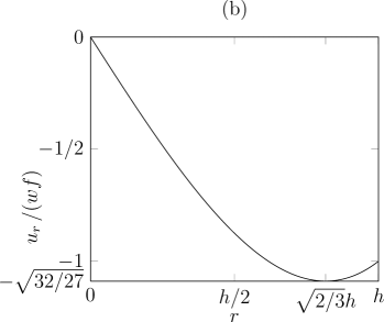
Figure 2: Flow in a cylindrical tube of radius $h$. (a) Axial flow velocity $u_{z}$ given in Eq. (38) plotted as a function of radial position $r$. (b) Radial flow velocity $u_{r}$ given in Eq. (37) plotted as a function of radial position $r$. Note that the radial velocity has a minimum at $r=\sqrt{2/3}h\simeq 0.817\,h$ where the value is $u_{r}(\sqrt{2/3}h)=-\sqrt{{32}/{27}}wf\simeq-1.09\,wf(z)$.

Consider the flow in a cylindrical tube of radius $h$ as sketched in Fig. 1(c). Let the normal velocity at the wall be $u_{r}(h)=-wf(z)$. Assuming rotational symmetry of the velocity field, the governing equation (30) is

$$\left(\partial_{r}^{4}+\frac{2}{r}\partial_{r}^{3}+\frac{1}{r^{2}}\partial_{r}^{2}+\frac{1}{r^{3}}\partial_{r}\right)\phi=P$$ (33)

which has the solution

$$\phi=\frac{P}{64}r^{4}+\frac{1}{4}(2B_{2}-B_{3})r^{2}+(B_{1}+\frac{1}{2}r^{2}B_{3})\log r+B_{4}.$$ (34)

With $k=0$ at the $r=h$ channel wall, the boundary conditions in Eqns. (25)-(27) are

$$\frac{1}{r}\partial_{r}(r\partial_{r}\phi(h))=0,\quad\phi(h)=0,\quad-\partial_{r}\phi(h)=-w$$ (35)

Assuming further that the radial flow component vanishes at $r=0$ ($u_{r}(0)=0$) such that $-\partial_{r}\phi(0)=0$ we find for the for the velocity potential $\phi$ in Eq. (33)

$$\phi(r)=\left(-\frac{3h}{4}+\frac{r^{2}}{h}-\frac{r^{4}}{4h^{3}}\right)w.$$ (36)

The radial and axial velocity components can now be found from Eqns. (18)-(19)

$$u_{r} = -f\partial_{r}\phi=\frac{r\left(r^{2}-2h^{2}\right)w}{h^{3}}f,$$ (37)

$$u_{z} = F\frac{1}{r}\partial_{r}(r\partial_{r}\phi)=\frac{4(h^{2}-r^{2})w}{h^{3}}F$$ (38)

in agreement with e.g. Aldis (1988). The two velocity components are plotted in Fig. 2. We note that the radial velocity has a minimum at $r=\sqrt{2/3}h\simeq 0.817\,h$ where the value is $u_{r}(\sqrt{2/3}h)=-\sqrt{{32}/{27}}wf\simeq-1.09\,wf(z)$.

III.2 Flow between parallel plates

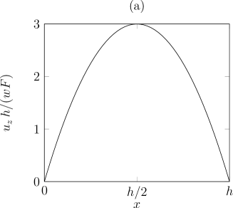
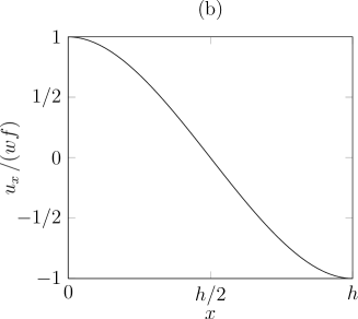
Figure 3: Flow between parallel porous plates located at $x=0$ and $x=h$ with boundary conditions $u_{x}(0)=wf$ and $u_{x}(h)=-wf$. (a) Axial flow velocity $u_{z}$ given in Eq. (46) plotted as a function of vertical position $x$. (b) Transverse flow velocity $u_{x}$ Eq. (45) plotted as a function of vertical position $x$.

Consider the flow between two infinite parallel plates located at $x=0$ and $x=h$ as sketched in Fig. 1(d). Let the normal velocity at the walls be $u_{x}(0)=w_{-}f(z)$ and $u_{x}(h)=w_{+}f(z)$. The governing equation (30) is

$$\partial_{x}^{4}\phi=P\\$$ (39)

which has the solution

$$\phi=A_{0}+A_{1}x+A_{2}x^{2}+A_{3}x^{3}+\frac{P}{24}x^{4}.$$ (40)

Applying the boundary conditions in Eqns. (25)-(27)

$$\partial_{x}^{2}\phi(0)=0,\quad\partial_{x}^{2}\phi(h)=0,\quad\phi(0)=0,\quad-\partial_{x}\phi(0)=w_{-},\quad\text{and}\quad-\partial_{x}\phi(h)=w_{+},\quad$$ (41)

yields

$$\phi=\frac{(w_{-}-w_{+})x^{3}}{h^{2}}+\frac{(w_{+}-w_{-})x^{4}}{2h^{3}}-w_{-}x.$$ (42)

The transverse and axial velocity components can be found from Eqns. (18)-(19)

$$u_{x} = -f(z)\partial_{x}\phi=\left(\frac{3(w_{+}-w_{-})x^{2}}{h^{2}}+\frac{2(w_{-}-w_{+})x^{3}}{h^{3}}+w_{-}\right)f$$ (43)

$$u_{z} = F(z)\partial_{x}^{2}\phi=\frac{6(w_{-}-w_{+})(h-x)x}{h^{3}}F$$ (44)

The solution for the special case $w_{-}=-w_{+}=w$ is shown in Fig. 3. In that case the velocity components are

$$u_{x} = \frac{h^{3}-6hx^{2}+4x^{3}}{h^{3}}wf,$$ (45)

$$u_{z} = \frac{12(h-x)x}{h^{3}}wF.$$ (46)

These were first by obtained Berman (1953) who considered the case $f=1$.

III.3 Flow in an equilateral triangle

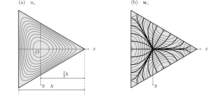
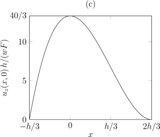
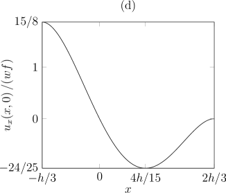
Figure 4: Flow in a porous tube whose cross-section is an equilateral triangle of height $h$ and side length $2h/\sqrt{3}$. (a) Contour lines for the axial flow velocity field $u_{z}(x,y)$. The contour lines are shown in steps of $10\%$ of the maximum value. (b) Stream(thick)- and contour(thin) lines for the transverse velocity field $\boldsymbol{u}_{\perp}=(u_{x},u_{y})$. The contour lines show the velocity magnitude $|\boldsymbol{u}_{\perp}|$ in steps of $10\%$ of the maximum value. (c) A plot of $u_{z}(x,0)$ along the centerline parallel to the $x$-axis. (d) A plot of $u_{x}(x,0)$ along the centerline parallel to the $x$-axis.

Consider the flow of liquid in a porous channel whose cross-section is an equilateral triangle of height $h$ and side length $2h/\sqrt{3}$, as shown in Fig. 1(e). Let the normal wall velocity be given by $u_{w}=w(x,y)f(z)$, and let the mean value of $w(x,y)$ when averaged over the channel wall be $w_{0}$. The governing equation (30) is

$$(\partial^{2}_{x}+\partial^{2}_{y})^{2}\phi=P,$$ (47)

while the boundary conditions in Eqns. (25)-(27) are

$$\partial^{2}_{n}\phi=0,\quad\phi=0,\quad\text{and}\quad\quad-\partial_{n}\phi=w.$$ (48)

The solution of Eq. (47) with the boundary conditions $\partial^{2}_{n}\phi=0$ and $\phi=0$ is

$$\phi=\frac{P}{64h}\left(x^{3}-3y^{2}x-h(x^{2}+y^{2})+\frac{4}{27}h^{3}\right)\left(\frac{4}{9}h^{2}-x^{2}-y^{2}\right)$$ (49)

The magnitude of the wall normal flow velocity $u_{w}=w(x,y)f(z)$ is the same on each of the three boundaries. At the $x=-{h}/{3}$ wall we find

$$u_{x}(-h/3,y)=\left.-f\partial_{x}\phi(x,y)\right|_{x=-h/3}=-\frac{P\left(h^{2}-3y^{2}\right)^{2}}{192h}f.$$ (50)

The mean velocity (when averaged over the $x=-h/3$ boundary) is $-{h^{3}Pf}/{360}$ so by choosing $P=-{360w_{0}}/{(h^{3})}$, the average inflow velocity becomes $w_{0}f$. Using $P=-{360w_{0}}/{(h^{3})}$ in Eq. (49), the velocity components can be found from Eqns. (18)-(19) recalling that $u_{x}=-f\partial_{x}\phi$, $u_{y}=-f\partial_{y}\phi$ and $u_{z}=F(\partial^{2}_{x}+\partial^{2}_{y})\phi$

$$u_{x} = \frac{5\left(18\left(6hx+9x^{2}-2h^{2}\right)y^{2}+81y^{4}-x(8h+15x)(2h-3x)^{2}\right)}{24h^{4}}w_{0}f$$ (51)

$$u_{y} = -\frac{5(h+3x)y\left(8h^{2}-6ax-9\left(x^{2}+3y^{2}\right)\right)}{6h^{4}}w_{0}f$$ (52)

$$u_{z} = \frac{10(h+3x)\left((2h-3x)^{2}-27y^{2}\right)}{3h^{4}}w_{0}F$$ (53)

The velocity field is shown in Fig. 4.

III.4 Flow in an rectangular channel

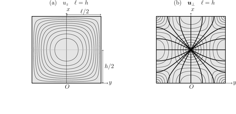
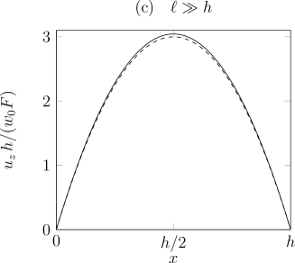
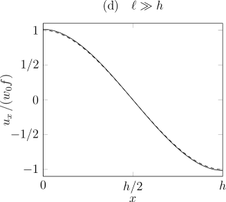
Figure 5: Flow in a rectangular porous tube with sides of length $h$ and $\ell$. (a) Contour lines for the axial flow velocity field $u_{z}(x,y)$ for the case $h=\ell$. The contour lines are shown in steps of $10\%$ of the maximum value. (b) Stream(thick)- and contour(thin) lines for the transverse velocity field $\boldsymbol{u}_{\perp}$ for $h=\ell$. The contour lines show the velocity magnitude $|\boldsymbol{u}_{\perp}|$ in steps of $10\%$ of the maximum value. (c) A plot of $u_{z}(x,0)$ (solid line) along the centerline parallel to the $x$-axis for $\ell/h=1000$. Dashed line shows $u_{z}(x,0)$ for parallel plates, c.f. Eq. (46). (d) A plot of $u_{x}(x,0)$ (solid line) along the centerline parallel to the $x$-axis $\ell/h=1000$. Dashed line shows $u_{x}(x,0)$ for parallel plates, c.f. Eq. (45). In (a) and (b), the first $100$ terms in Eqns. (55)–(57) were used.

Consider the flow in a porous channel whose cross-section is a rectangle with sides of length $h$ and $\ell$ centered at $(x,y)=(0,h/2)$ as shown in Fig. 1(d). Let the normal wall velocity be given by $u_{w}=w(x,y)f(z)$, and let the mean value of $w(x,y)$ when averaged over the channel walls be $w_{0}$.

The equations of motion and boundary conditions are once again given by Eqns. (47)-(48). As we need to evaluate the first and second order $x$ and $y$-derivatives to determine the velocity field, Levy’s solution of the corresponding plate bending problem is convenient

$$\phi = \frac{4Ph^{4}}{\pi^{5}}\sum_{n=1,3,\ldots}\frac{1}{n^{5}}\left(1-\mathcal{A}_{n}\cosh\frac{2\alpha_{n}y}{\ell}+\mathcal{B}_{n}y\sinh\frac{2\alpha_{n}y}{\ell}\right)\sin\frac{n\pi x}{h}$$ (54)

where $\alpha_{n}={n\pi\ell}/({2h})$, $\mathcal{A}_{n}=({\alpha_{n}\tanh\alpha_{n}+2})/({2\cosh\alpha_{n}})$, and $\mathcal{B}_{n}={\alpha_{n}}/({\ell\cosh\alpha_{n}})$. From Eqns. (54), (18), and (19) we may calculate the velocity components

$$u_{x} = -\frac{4Ph^{3}}{\pi^{4}}f\sum_{n=1,3,\ldots}\frac{1}{n^{4}}\left(1-\mathcal{A}_{n}\cosh\frac{2\alpha_{n}y}{\ell}+\mathcal{B}_{n}y\sinh\frac{2\alpha_{n}y}{\ell}\right)\cos\frac{n\pi x}{h}$$ (55)

$$u_{y} = -\frac{4Ph^{4}}{\pi^{5}}f\sum_{n=1,3,\ldots}\frac{1}{n^{5}}\left(-\frac{2\alpha_{n}}{\ell}\mathcal{A}_{n}\sinh\frac{2\alpha_{n}y}{\ell}+\mathcal{B}_{n}\left(\sinh\frac{2\alpha_{n}y}{\ell}+\frac{2\alpha_{n}}{\ell}y\cosh\frac{2\alpha_{n}y}{\ell}\right)\right)\sin\frac{n\pi x}{h},$$

(56)

$$u_{z} = -\frac{4Ph^{2}}{\pi^{3}}F\sum_{n=1,3,\ldots}\frac{1}{n^{3}}\left(1-\frac{\cosh\frac{n\pi y}{h}}{\cosh\alpha_{n}}\right)\sin\frac{n\pi x}{h}$$ (57)

To determine $P$ such what the average inflow velocity is $w_{0}f$, we solve for $P$ in

$$\frac{2}{h}\int_{0}^{h}u_{y}(-\ell/2,x,z)\;\mathrm{d}x+\frac{2}{\ell}\int_{-\ell/2}^{\ell/2}u_{x}(0,y,z)\;\mathrm{d}y=w_{0}f.$$ (58)

In the following we determine $P$ for the special cases $\ell=h$ and $\ell\gg h$.

III.4.1 The case $\ell=h$

To determine the velocity field in the case $\ell=h$ we note that the sums in Eqns. (55)–(57) converge very rapidly, and that the flow profile $u_{x}(0,y)$ at the $x=0$ wall is well approximately by the first term in Eq. (55)

$$u_{x}(0,y,z) \simeq -\frac{4Ph^{3}}{\pi^{4}}\left(1-\mathcal{A}_{n}\cosh\frac{2\alpha_{n}y}{\ell}+\mathcal{B}_{n}y\sinh\frac{2\alpha_{n}y}{\ell}\right)f$$ (59)

From Eq. (58) we therefore find

$$\frac{4}{\ell}\int_{-\ell/2}^{\ell/2}u_{x}(0,y,z)\;\mathrm{d}y\simeq-\frac{8h^{3}P}{\ell\pi^{5}}{\left(\,\text{sech}\,\frac{\ell\pi}{2h}\right)^{2}\left(\ell\pi\left(2+\cosh\frac{\ell\pi}{h}\right)-3h\sinh\frac{\ell\pi}{h}\right)}f=w_{0}f,$$ (60)

which determine $P$ as a function of the average normal flow velocity $w_{0}$

$$P=-\frac{\pi^{5}}{16}\frac{1+\cosh\pi}{\pi(2+\cosh\pi)-3\sinh\pi}\frac{w_{0}}{h^{3}}\simeq-29.90\frac{w_{0}}{h^{3}}$$ (61)

Summing the first $100$ terms in Eqns. (55)-(56) we find from Eq. (58) that $P=-28.46\,{w_{0}}/{h^{3}}$ so the error in the expression for $P$ in Eq. (61) is less than $5\%$. The velocity field for $\ell=h$ is shown in Fig. 5(a-b).

III.4.2 The case $\ell/h\gg 1$

To determine the velocity field in the case $\ell\gg h$ we again use Eq. (59). Near the centerline parallel to the $x$-axis, i.e. for $|y|\ll\ell$, we find from Eq. (59) that the wall velocity $u(0,0,z)\simeq-{4Ph^{3}f}/{\pi^{4}}$ so with $P=-\pi^{4}w_{0}/(4h^{3})$ the condition in Eq. (58) is fulfilled. For the transverse velocity $u_{x}$ along the centerline $y=0$ we obtain from Eq. (55)

$$u_{x}(x,0,z)=w_{0}f\sum_{n=1,3,\ldots}\frac{1}{n^{4}}\cos\frac{n\pi x}{h}.$$ (62)

This series can be summed

$$u_{x}(x,0,z)=\frac{\pi^{4}}{96}\frac{h^{3}-6hx^{2}+4x^{3}}{h^{3}}w_{0}f.\\$$ (63)

The prefactor $\pi^{4}/96\simeq 1.01$, in good agreement with Eq. (45). Similarly, we find from Eq. (57)

$$u_{z}(x,0,z)=\frac{\pi^{4}}{8}\frac{(h-x)x}{h^{3}}w_{0}F$$ (64)

The prefactor ${\pi^{4}}/{8}\simeq 12.18$ in good agreement with Eq. (46). The velocity field for $\ell\gg h$ is shown in Fig. 5(c-d).

IV Conclusion

We have analyzed slow flow in channels with porous walls. A similarity transformation reduces the Navier-Stokes equations to a set of coupled equations for the velocity potential in two dimensions. We have shown that when the Reynolds number and channel aspect ratio is small, an analogy exists between flow in channels with porous walls and bending of simply suspended plates under uniform load. If a solution of the problem of a suspended plate has been obtained, a problem of viscous motion in a porous tube has thus also been solved. We have applied this result to flow in rectangular and triangular channels. Our results provide a general framework for the extension of Berman flow (Berman, 1953) to three dimensions.

V Adknowledgements

The author acknowledge many fruitful discussions with Hassan Aref and Tomas Bohr. This work was supported by the Materials Research Science and Engineering Center (MRSEC) at Harvard University.

References

- Aldis (1988) Aldis, G.K. 1988 The unstirred layer during osmotic flow into a tubule. Bulletin of Mathematical Biology 50 (5), 531–545.
- Batchelor (1967) Batchelor, G. K. 1967 An Introduction to Fluid Dynamics. Cambridge University Press.
- Berman (1953) Berman, A. S. 1953 Laminar Flow in Channels with Porous Walls. Journal of Applied Physics 24 (9), 1232–1235.
- Berman (1958) Berman, A. S. 1958 Laminar Flow in an Annulus with Porous Walls. Journal of Applied Physics 29 (1), 71–75.
- Cox (1991) Cox, S. M. 1991 Two-dimensional flow of a viscous fluid in a channel with porous walls. Journal of Fluid Mechanics 227, 1–33.
- Holbrook & Zwieniecki (2005) Holbrook, N. M. & Zwieniecki, M., ed. 2005 Vascular transport in plants. Academic Press.
- LaBarbera (1990) LaBarbera, M. 1990 Principles of Design of Fluid Transport Systems in Zoology. Science 249 (4972), 992.
- Lauga et al. (2004) Lauga, E., Stroock, A. D. & Stone, H. A. 2004 Three-dimensional flows in slowly varying planar geometries. Physics of Fluids 16 (8), 3051.
- Meleshko (1996) Meleshko, V. V. 1996 Steady Stokes flow in a rectangular cavity. Proceedings of the Royal Society of London 452 (1952), 1999–2022.
- Nielsen (2012) Nielsen, C H, ed. 2012 Biomimetic Membranes for Sensor and Separation Applications. Springer.
- Rayleigh (1893) Rayleigh, L. 1893 On the flow of viscous liquids, especially in two dimensions. Philos. Mag 5, 354–372.
- Richards (1960) Richards, T. H. 1960 Analogy between the slow motion of a viscous fluid and the extension and flexure of plates: a geometric demonstration by means of moire fringes. British Journal of Applied Physics 11, 244.
- Schlichting & Gersten (2000) Schlichting, H. & Gersten, K. 2000 Boundary Layer Theory. Springer.
- Taylor (1923) Taylor, G. I. 1923 On the decay of vortices in a viscous fluid. Philosophical Magazine 46 (274), 671–674.
- Timoshenko (1964) Timoshenko, S. 1964 The Theory of Plates and Shells. McGraw-Hill Publishing Company.
- Ventsel & Krauthammer (2001) Ventsel, E. & Krauthammer, T.b. 2001 Thin Plates and Shells: Theory, Analysis, and Applications. CRC Press.
- Yuan & Finkelstein (1956) Yuan, S. W. & Finkelstein, A. B. 1956 Laminar Pipe Flow with Injection and Suction Through a Porous Wall. Trans ASME 78, 719–724.