Quantum Field Theory and the Internal States of Elementary Particles

Abstract

A new application of quantum field theory is developed that gives a description of the internal dynamics of dressed elementary particles and predicts their masses. The fermionic and bosonic quantum fields are treated as interdependent fields satisfying coupled quantum field equations, all expressed at the same space-time coordinate. Quantization is realized by expanding the quantum fields in terms of fermionic creation and annihilation operators. This approach is applied in a QCD description of the light quarks with a zero Higgs field. Originally massless and pointlike, an isolated quark (described in its own center-of-mass) acquires mass and a finite extent when treated as an interacting system of quark and gluon fields. The binding mechanism of this localized system has a topological character, being a consequence of the non-linear nature of QCD, while being insensitive to the magnitude of the coupling constant to lowest order. To prevent this system from collapsing general relativity is introduced. The quark stabilizes at a radius of 8.8 Planck lengths and acquires a mass of 3.2 MeV, in remarkable agreement with accepted phenomenological values. It is suggested that the two higher generations of quarks are associated with the other two real solutions of the Higgs field equations.

I Introduction

The standard model has been extremely successful in describing scattering phenomena between elementary particles. Nonetheless, it is clear that this picture of Nature cannot be complete. Most importantly, the standard model contains too many free parameters to be called fundamental, and can thus best be seen as an effective theory. In modern treatments the masses of the standard model fermions are supposed to arise from the couplings of quarks to various Higgs fields, however, so far this has not lead to a reduction of the number of parameters. Of the 19 free parameters of the standard model, 13 belong to the Yukawa/Higgs sector Gabrielli . These parameters are put in by hand, and there is no explanation for the huge hierarchy of masses ranging over 6 orders of magnitude (not including the neutrinos). Further extensions beyond the standard model often lead to a greater - rather than a smaller - set of unknown parameters.

Given this situation one may wonder whether it is not possible to underlie the standard model by a theory at a more fundamental level that evolves into the standard model through the construction of effective solutions of the bare degrees of freedom. Such an underlying theory should contain many of the elements of the standard model but have a simpler structure, i.e. it should embody a certain unification of the diverse elements of the effective theory. The simplicity should imply fewer degrees of freedom and fewer parameters at the fundamental level. The new application of QFT methods, introduced in this paper, enables such a link between fundamental and effective levels by its ability to construct massive dressed elementary particles from more fundamental bare massless particles.

An important element of such a fundamental theory could be the reduction of the three generations in the effective theory to a single one in the fundamental theory. Since the three generations in the standard model are not associated with any additional symmetry or interaction, three generations may well be the result of multiple solutions at a more fundamental level. This possible scenario would gain in standing if we could explain the emergence of (exactly) three generations from the exact level. We suggest that a single fundamental Higgs field might explain the threefold split. The Higgs field equations would typically have three real solutions, whose classical approximations could be denoted by $\phi=0$ and $\phi=\pm\sqrt{|\mu^{2}/\lambda|}$. In the quark-Higgs dynamics the positive and negative solutions lead to distinct solutions, so that these three solutions would indeed lead to three distinct fermion sectors. Since the nature of the Higgs Lagrangian at the fundamental level is not (yet) unambiguously established and a non-zero Higgs field would complicate our basic model considerably, we limit ourselves in this paper to the trivial Higgs solution, namely $\phi=0$. However, this also eliminates the Higgs parameter $\mu$ from the model, so that it is unclear how this basic theory acquires a scale. The question of the basic scale parameters in Nature has been considered in the context of cosmology elsewhere Greben . We find that for the light quarks general relativity has to be introduced to ensure the existence of the quarks, so that for this basic generation the cosmological parameters reviewed in Greben also play a role. The presence of different scale parameters at this fundamental level could give a possible explanation of the hierarchy problem in physics, as it would allow for the existence of a range of different scales at a very basic level.

Which further ingredients would survive in a fundamental theory underlying the standard model? It is to be expected that the SU(3) theory of strong interactions will survive, as this theory is unbroken at the standard model level and is not characterized by a complex multiplet structure. The complexities of the multiplet structure and broken symmetries in the standard model originate from the electro-weak interaction and it is not clear which of these complexities emerge in the transition from fundamental to effective theory, or which ones are already present at the most fundamental level. Therefore it is natural to limit oneself originally to QCD. Clearly, so long as one does not consider the electro-weak interactions one cannot describe leptons as effective systems, so we also focus on quarks in this paper. Being a non-linear theory, one expects that QCD can supply the necessary self-consistent binding mechanism for the effective quark system, recalling the important role non-linear dynamics plays in soliton particle models in hadron physics Rajaraman . By adding the electromagnetic interaction at a later stage one can break the isospin symmetry of QCD and try to explain the mass differences between up and down quarks. Being a linear theory, the electromagnetic force can be treated perturbatively and is not expected to interfere with the expected non-linear binding mechanism, so that it can be ignored initially.

As stated before, the possibility to link the dressed particles and their internal properties and masses to more fundamental bare particles relies on a new methodology which emphasizes the use of the field equations in QFT. The standard applications of quantum field theory (QFT) deal with scattering processes expressed in term of propagators and vertices, yielding the well-known Feynman diagrams. The dressing of fermions is then expressed in a series of time-ordered interaction diagrams modifying the bare propagator. Most of these diagrams are divergent, which has necessitated the renormalization methods to arrive at meaningful physical results, although outside inputs are still required to fix the physical parameters. This dressing process does not yield any internal properties of the particles, due to the fact that the fermions interact with external bosonic fields. The dressing process which is introduced in this paper is of a very different nature as the fermionic and bosonic fields are treated as mutually dependent fields, the dependence being controlled by the coupled field equations. Hence, the boson fields are not treated as external fields and all fields and interactions refer to the same space-time coordinate. It is this treatment that enables one to describe the internal properties of elementary particles.

It is clear that the field equations play a dominant role in the new formulation. This is not unlike most other areas of physics. However, in QFT their use has been very limited to date. Often the field equations in QFT are denoted as classical, and indeed they are often used as such. For example, the scalar Higgs field $\phi$ satisfies a classical field equation with various (constant) classical solutions. The ”full” solution is then expanded around this classical solution, and only the additional fields are quantized. Despite their classical nature the constant solutions are attributed physical meaning, and their value is often denoted as the vacuum expectation value of the Higgs field Gabrielli . This is a dubious use of the term expectation value as it suggests that one takes the expectation value of an operator, which one does not. It is not sufficient to call something an operator, one also has to treat it as such. The expansion around classical solutions is also common in the soliton and instanton problem Rajaraman . Here the basic solution also satisfies an approximate non-linear classical equation of motion, and quantization is imposed by linearizing the remainder. We feel that these procedures are fundamentally flawed. If classical solutions have any role to play in QFT then they should emerge as an approximation to the quantum operators, not lie at the basis of the quantization procedure. Quantization should be done up front, not as an afterthought. Hence, we promote a much more rigorous quantum-mechanical use of the field equations. Before solving the field equations one should turn them into quantum equations and ensure that the solutions are quantum field operators.

A rigorous quantization procedure can be realized by turning the classical fields into quantum fields by expanding them into creation and annihilation operators, the latter satisfying well-defined (anti-) commutation rules. The insertion of quantum operators in the field equations also means that the order of the fields in the field equations can make an important difference, a phenomenon well-known in most quantization procedures. Hence, before solving the field equations one must establish the correct order of the fields. This is usually possible by demanding consistency, by imposing symmetries or through other physical requirements. At this point it is of interest to review the standard quantization procedure for a linear field theory such as QED, since this may elucidate why classical solutions have played such a prominent role in traditional quantization procedures, a role which should be avoided when one deals with non-linear equations. To derive the electromagnetic field operator in QED one first determines the classical solutions of the classical linear equation (plane waves in the free case). One then quantizes the field by appending creation and annihilation operators to the classical solutions. This well-known procedure leads to the correct quantized electromagnetic field, and therefore may well be responsible for the practice to use classical solutions in the quantization procedure. However, we would have reached the same result by inverting the order, namely, by first expanding the field in terms of creation and annihilation operators of (as yet) unknown functions, and then solve the (quantum) equations of motion. This procedure would yield the same plane wave states. However, by choosing this latter order one guarantees up front that the solutions are quantum solutions. For non-linear field equations it makes a huge difference which order is applied. If one solves the non-linear equations classically, and then appends creation and annihilation operators to these solutions, then the resulting operator is generally no longer a solution of the quantum field equations, as the operators do not behave like c-numbers. Hence, one must first introduce the field operators and then construct operator solutions to the field equations. If the resulting profile functions, which multiply the creation or annihilation operators, are identical - or close - to the classical solutions, then this could justify a classical approximation. However, such a situation only arises if the resulting field operator acts like a unit operator in operator space. In general this situation does not apply and classical solutions cannot be expected to play a fundamental role in non-linear field theories.

As indicated above, creation and annihilation operators play a central role in the quantization procedure. The operator nature of the field now even becomes part of the solution process and in general the simple linear expansion of the fermion and boson fields in terms of creation and annihilation operators is no longer a solution of the full set of field equations. One can start with the simple linear expansion of the fermion field, however, after further iterations a much more complex structure will evolve. For example, to lowest order the gluon operator becomes a bilinear operator in terms of the fermionic creation and annihilation operators. This bilinear expansion of the gluon field in terms of fermionic operators, instead of in single bosonic creation and annihilation operators, does not imply that gluon fields have lost their identity. In fact a similar expansion of the gluon field (or the photon field for that matter) in terms of quark operators is possible when it is considered an external field (and thus fully independent field) and satisfies the homogeneous gluon field equations. So such an expansion in fermionic degrees of freedom is perfectly consistent with the idea of independent gluons, soft gluons and glueballs. However, in the self-consistent case, which we are considering here, the gluon and quark fields are interdependent and neither of these fields can be considered as independent, although it still makes sense to talk about the fermion and gluon degrees of freedom. One should also not interpret this formal expansion of the gluon field as a composite model of the gluon. It is known that the quark-antiquark interaction is repulsive in the color octet gluon channel, however, forces play no role in the operator expansion and this fact plays no role in the expansion.

By further iteration one can construct the whole operator structure of the exact quantum fields. Ultimately one arrives at an infinite sum of operator terms, each additional term containing a higher power of creation and annihilation operators. Despite the elaborate operator structure of the fields and the equations it is possible to construct a closed operator solution. In Section II and Appendix A, this complete operator structure of the fields is derived and is expressed in an elegant concise form, involving a vacuum projection operator. By factoring out the quantum operators the quantum field equations can then be reduced to ordinary coupled equations, similar in structure - but not in content - to the classical equations. The elegance of this reduction is further underlined by the fact that the number of profile functions remains finite, despite the infinite nature of the expansion. The dependence on spin, color and isospin can also be factored out, leaving in the end a set of coupled differential equations for c-number profile functions. The number of profile functions depends on the symmetries present: for our QCD formulation there are only 5 gluon profile functions. But if symmetries are broken (like isospin in QED), more profile functions are needed. One of the great unexpected benefits of this quantum reduction is that the resulting non-linear equations are more amenable to analytic solutions than the original classical field equations.

After further extensive manipulations of the scalar coupled equations, two simple order $\textrm{O}(\alpha_{s}^{0})$ solutions emerge. The first one is an uninteresting ”trivial” solution, in which all effective potentials vanish. The second one features non-zero potentials that become singular at a finite radius $r_{0}$. This absolute confining mechanism of the quark within its self-generated bag is of great beauty and is made possible by a unique QFT mechanism not seen before in particle theory. Since this solution is enabled by the non-linear nature of the field equations and is independent of the coupling constant, it will be denoted as a topological binding mechanism. However, this solution still features some other problems. First, in the absence of a Higgs field (we set $\phi=0$) this QCD model does not contain a scale, so there is no indication whether this model refers to a real particle. A second problem is that the expectation value of the energy operator is negative, so that this energy cannot be identified with the mass of the quark. In addition, a system with negative energy will collapse to a point as this minimizes its energy. These problems have an amazing solution. By linking QCD to general relativity (GR), we can exploit the fact that GR contains a definite scale and that gravity will act as a repulsive force if the energy of the system is negative. Hence, after the system has contracted to the Planck scale the repulsive gravitational force becomes big enough to halt the collapse. By adding vacuum energy Greben10 to the system we can compensate for the negative internal energy, and eventually obtain a net positive energy that can be identified with the mass of the system. Amazingly, this mass comes out to be slightly over 3 MeV, which is close to the phenomenological values found for the light quark masses. Hence, this solution can be identified with the light quark doublet. This solution also resolves the apparent conflict between the smallness of the quark mass and its pointlike nature. Normally, a mass of 3 MeV would correspond to a ridiculous size of 65 fm, but our result of 8.8 Planck lengths lies well within observable limits.

Now that we have explained the basic elements in our formulation of the internal bound state dynamics of QFT, it is appropriate to mention earlier approaches in QFT that tried to describe localized states. Soon after the development of the Dirac equation, this equation was used to carry out bound-state calculations, for example by deriving relativistic corrections to the non-relativistic hydrogen atom calculations. The success of these calculations already suggested that QFT can be used fruitfully in bound-state problems, however, the nature of these Dirac calculations (the proton is not treated as a quantum field) shows that such a calculation cannot really be called a genuine QFT calculation. Historically, the electron also has been subjected to bound-state calculations of quantum nature. Schweber paper1 reviews efforts to describe the electron as a bound state in the period 1940-1955. Dirac paper2 made an attempt to describe an electron as a particle with a finite, perfectly conducting, surface in 1962. However, these efforts were hampered by the fact that the electroweak and strong gauge theories had not yet been developed at the time, while one can expect that the non-linearity of these non-Abelean gauge theories is essential for the construction of bound-state solutions. Other methods have been developed to handle bound-state problems within standard QFT, for example, the Bethe-Salpeter equations (Bethe , Gell-Mann , Gross , Mitra , Mitra2 ), the Blankenbecler-Sugar equations Sugar , and the Dyson-Schwinger equations paper4 . However, none of these theories could describe the internal properties of the elementary particles as the bosonic fields were treated as external fields. More recently, lattice gauge calculations have been applied to nucleons considered as assemblies of quarks Proton_mass . However, these calculations are also not designed to give insights in the quarks and leptons themselves.

Historically, our efforts to solve the non-linear QCD field equations self-consistently started out as an attempt to describe the binding of three quarks in a bag, expecting to develop an alternative to the bag models popular in the eighties Bag_model . Solutions were found fairly quickly paper9 , however, their physical interpretation left much to be desired as the mass/energy scale of the light quarks (a few MeV) corresponds to very extensive objects, which are physically unacceptable. Also, only particle states were considered initially, as was common in the field of intermediate energy physics Araki and other papers dealing with pion corrections to quark bag models Bag_model . It soon became clear that it is difficult to apply such an approach without anti-particles consistently, and this initial approach was replaced by a formulation in which all fields are expanded in particle and anti-particle creation and annihilation operators. When this formulation lead to the exact operator solution it also became clear that this approach cannot be used for composite systems such as three quark bags, as the operator solutions only survive if they operate on one-body state vectors. Hence, the attention switched from describing composite systems to elementary particles and this led to the realization that these new QFT methods can be used to give a description of the internal dynamics of elementary particles, in particular quarks.

The outline of the paper is as follows. In Section II we discuss the equations of motion and derive the form of the field operators in terms of quark creation and annihilation operators. The formal solution of these operator equations is presented, allowing the reduction of the field equations to ordinary differential equations. After defining the c-number wave function components and c-number gluon profile functions in Section III, we describe the form of the ordinary second-order differential equations, controlling the behaviour of the gluon profile functions in Section IV. These equations are highly non-linear, and at first sight look fairly untractable. However, after introducing a reduction process in Section V, we can cast these equations in an elegant symmetrical form, which allows simple solutions to zeroth order in $\alpha_{s}$. The linear equations for $\textrm{O}(\alpha_{s})$-corrections are also derived. In Section VI we discuss the (Dirac-like) field equation for the quark and the form of the potentials. In Section VII a self-consistent solution of the coupled quark-gluon equations is presented. In Section VIII we discuss the evaluation of expectation values for the energy, spin and colour of the quark system. These allow us to define sufficient boundary conditions to determine the parameters of the solutions uniquely. In Section IX we discuss the necessity to include coupling to GR for the trivial Higgs sector. By incorporating vacuum energy as well, one is able to make precise estimates of the quark mass and radius. In the final section X we summarize the significance of these results and discuss a possible steps for deriving the internal properties and masses of other particles in the standard model.

II The Quantization of the Equations of Motion in Quantum Chromodynamics (QCD)

As stated before we start from a basic QCD Lagrangian paper6 without electro-weak and Higgs interactions:

$$\mathcal{L}=\bar{\psi}(\textrm{i}\gamma_{\mu}D^{\mu}-M)\psi-\frac{1}{4}\textbf{F}^{\mu\nu}\bullet\textbf{F}_{\mu\nu},$$ (1)

where the covariant derivative is defined as follows:

$$D^{\mu}=\partial^{\mu}-\frac{1}{2}\textrm{i}g_{s}\boldsymbol{\lambda}\bullet\textbf{A}^{\mu}.$$ (2)

Here the $\lambda_{a}$ are the Gell-Mann $SU(3)$-matrices. The inproducts run over 8 components:

$$\textbf{A}\bullet\textbf{B}=\sum_{a=1}^{8}A_{a}B_{a}.$$ (3)

The gluon field tensor is given by the expression:

$$\textbf{F}^{\mu\nu}=\partial^{\mu}\textbf{A}^{\nu}-\partial^{\nu}\textbf{A}^{\mu}+g_{s}\textbf{A}^{\mu}\times\textbf{A}^{\nu}.$$ (4)

Here, the $SU(3)$ vector product is defined by:

$$\left(\textbf{A}\times\textbf{B}\right)_{a}=\sum_{b,c=1}^{8}f_{abc}A_{b}B_{c},$$ (5)

where the $f_{abc}$ are the $SU(3)$ structure constants. The classical equations of motion for the gluon fields are given by:

$$\partial_{\mu}\textbf{F}^{\nu\mu}(x)=\frac{1}{2}g_{s}\bar{\psi}(x)\boldsymbol{\lambda}\gamma^{\nu}\psi(x)+g_{s}\textbf{F}^{\nu\mu}(x)\times\textbf{A}_{\mu}(x),$$ (6)

while the equation of motion for the quark field is:

$$\left(\textrm{i}\gamma_{\mu}\partial^{\mu}+\frac{1}{2}g_{s}\gamma_{\mu}\lambda_{a}A_{a}^{\mu}(x)-M\right)\psi(x)=0.$$ (7)

In the standard applications of QFT, the fermion and boson fields are expanded in the eigenstates of the free Hamiltonian, while the interaction Hamiltonian is used to calculate the scattering diagrams in the perturbative Feynman series. Its main application lies in scattering problems, and the fermion masses are put in by hand. In the current application of QFT we start from a more basic level where the bare fermions have zero masses (i.e. we set $M=0$), and we try to solve the full set of field equations self-consistently for a particular (quark) state vector. The quark is described in its own center-of-mass system (the origin of the coordinate system), and characterized by localized profile functions representing either the gluon fields or internal quark wave function. The actual position of the system that describes the effective particle is thus irrelevant and only becomes of relevance when we enter the quark into the multi-particle environment and consider scattering processes.

Quantization of the formulation is accomplished by expanding the fields in terms of creation and annihilation operators, the latter satisfying certain (anti-) commutation relations. Initially the following expansion of the quark fields is used:

$$\psi(x)=\sum_{\alpha}b_{\alpha}\phi_{\alpha}(x)+\sum_{\alpha}d_{\alpha}^{\dagger}\phi_{\alpha}^{a}(x),$$ (8)

where $b_{\alpha}$ is the quark annihilation operator, $d^{{\dagger}}_{\alpha}$ the anti-quark creation operator, and the profile functions $\phi_{\alpha}(x)$ and $\phi^{a}_{\alpha}(x)$ loosely refer to the particle and anti-particle wave functions of the quark in its own center-of mass system (i.e. the internal wave functions). These wave functions are not known beforehand, and even their existence is uncertain, since it is not known whether a localized system description of the quark state $b_{\alpha}^{\dagger}|0\rangle$ will emerge from the formulation. Since the field equations are solved self-consistently, only one space-time coordinate $x$ enters the considerations, so transitions between states are not associated with different times, and the overall state vector $b_{\alpha}^{\dagger}|0\rangle$ stays the same. Hence, the creation and annihilation operators are also time independent and do not evolve over time. The role of these creation and annihilation operators in the current formulation should be distinguished from that in scattering problems, where they are often associated with a particular fixed functional behavior (a plane wave corresponding to a particular positive or negative hyperboloid). When scattering states undergo time evolution through interactions they change their functional behavior, and creation and annihilation operators defined in this way are mixed up, allowing even the mixing of creation and annihilation operators (Bogoliubov mixing Bogoliubov ). In our formulation the creation and annihilation operators refer to the actual physical state, represented by $b_{\alpha}^{\dagger}|0\rangle$. Isolated particles do not change over time (unless they are unstable) and their state does not depend on where they are located, so $b_{\alpha}^{\dagger}$ has no space-time dependence. Only, when we use an external representation of the particles and specify their momentum and/or positions with respect to other particles in scattering processes, could we contemplate time dependent creation and annihilation operators to represent the time evolution of the world state vector. However, even in that case a time independent representation of these operators seems more appropriate in QFT, as the continuous evolution of the physical system between transitions is well represented by the continuous profile functions. The evolution of one world state to another through transitions is of a stochastic nature, and should not be represented by changing creation and annihilation operators. Rather transition operators (e.g. Feynman diagrams) should relate initial and final states uniquely defined in terms of fully specified creation and annihilation operators, i.e. time-dependent operators. Clearly, in our formulation no Bogoliubov mixing occurs, and particle and anti-particle components maintain their unique meaning. This is also important for the later developments in the theory, when we make an important distinction in the algebraic properties of particle and anti-particle operators to restore the symmetry between these entities which is broken in the Lagrangian formulation. In our operator formulation the vacuum also maintains its unique identity as the state without any particles present.

We now continue the discussion of Eq.(8). The index $\alpha$ covers the usual quantum numbers of the standard model: spin, color and charge (also called flavor, but we only consider one generation of quarks). Since we limit ourselves to QCD, we can treat the pair of quark states in each generation as a degenerate isospin doublet. The family/generation quantum number is supposed to be explained by the multiplicity of the solutions and is therefore absent. Both isospin and total angular momentum are good quantum numbers in the present formulation, so that we can limit the wave function space accordingly in the description of the quark state. Since the gluon fields carry color and spin, color and spin transitions can take place, and an expansion in terms of a complete set of color and spin states is required. No expansions in other quantum numbers, such as a principal quantum number, is appropriate since if a multiple of such states exist they should follow as a solution from the given equations, rather than appear in the expansion.

If we use the expansion, Eq.(8), in the gluon field equation Eq.(6), then the gluon field operators also become expansions in quark creation and annihilation operators. In first instance this expansion looks like:

$$A_{a}^{\mu}=\sum_{\alpha,\beta}b_{\alpha}^{\dagger}b_{\beta}A_{a,\alpha\beta}^{\mu,pp}+\sum_{\alpha,\beta}d_{\alpha}d_{\beta}^{\dagger}A_{a,\alpha\beta}^{\mu,aa}$$

$$+\sum_{\alpha,\beta}b_{\alpha}^{\dagger}d_{\beta}^{\dagger}A_{a,\alpha\beta}^{\mu,pa}+\sum_{\alpha,\beta}d_{\alpha}b_{\beta}A_{a,\alpha\beta}^{\mu,ap}.$$ (9)

However, the reinsertion of this expression in the Dirac equation, Eq.(7), leads to higher order terms in the expansion of $\psi(x)$, etc., which in turn leads to higher order terms in the expansion of the gluon field. It would thus seem that we have to revert to perturbative expansions, as is done in standard QFT. However, we will show below that the operator series can formally be summed to infinity, without increasing the number of profile functions.

To complete the quantization process we first recall the usual anti-commutation rules for the creation and annihilation operators:

$$\left\{b_{\alpha},b_{\beta}^{\dagger}\right\}=\delta_{\alpha,\beta},$$ (10)

and

$$\left\{d_{\alpha},d_{\beta}^{\dagger}\right\}=\delta_{\alpha,\beta},$$ (11)

while all other anti-commutators are zero. For free fields, when the fermion field is expanded in a complete set of plane waves, one can use these anti-commutation rules (i.e. their continuous generalizations) to derive the equal-time anti-commutator relations. For the current self-consistent treatment of the full set of coupled equations, such relations are absent. This shows that the anti-commutation rules Eqs. (10) and (11) are more fundamental than the equal-time anti-commutator relations. Historically one has often assumed the opposite, namely that the equal-time anti-commutator relations are fundamental to QFT (e.g. by stressing the analogy with the classical Poisson brackets), while Eqs. (10) and (11) were seen equivalent, but secondary. We have pointed out before that it is dangerous to rely on QFT on classical analogies, and this is a case in point.

Since the gluon field operator no longer commutes with the quark field operators, it is necessary to specify the order of the quark and gluon field operators in accordance with the symmetries and physical requirements of the theory. The non-commutativity of boson and fermion field operators is not new to QFT, for example Bjorken and Drell Bjorken discuss it in the context of QED. However, in the current context the consequences are must more farreaching. The anti-symmetric nature of the gluon field implies that we must replace Eq.(4) by:

$$\textbf{F}^{\mu\nu}=\partial^{\mu}\textbf{A}^{\nu}-\partial^{\nu}\textbf{A}^{\mu}+\frac{g_{s}}{2}\left\{\textbf{A}^{\mu}\times\textbf{A}^{\nu}-\textbf{A}^{\nu}\times\textbf{A}^{\mu}\right\}.$$ (12)

The quantized gluon field equations can be derived along similar lines and read:

$$-\partial_{\mu}\partial^{\mu}\textbf{A}^{\nu}+\partial^{\nu}\left(\partial_{\mu}\textbf{A}^{\mu}\right)=\frac{g_{s}}{2}\bar{\psi}\boldsymbol{\lambda}\gamma^{\nu}\psi$$

$$\left.+g_{s}\left\{\textbf{A}^{\mu}\times(\partial_{\mu}\textbf{A}^{\nu})-(\partial_{\mu}\textbf{A}^{\nu})\times\textbf{A}^{\mu}\right\}\right.$$

$$+\frac{g_{s}}{2}\left\{(\partial_{\mu}\textbf{A}^{\mu})\times\textbf{A}^{\nu}-\textbf{A}^{\nu}\times(\partial_{\mu}\textbf{A}^{\mu})\right.$$

$$\left.-\textbf{A}^{\mu}\times(\partial^{\nu}\textbf{A}_{\mu})+(\partial^{\nu}\textbf{A}_{\mu})\times\textbf{A}^{\mu}\right\}$$

$$-\frac{g_{s}^{2}}{4}\left\{\textbf{A}_{\mu}\times(\textbf{A}^{\nu}\times\textbf{A}^{\mu})-\textbf{A}_{\mu}\times(\textbf{A}^{\mu}\times\textbf{A}^{\nu})\right.$$

$$\left.-(\textbf{A}^{\nu}\times\textbf{A}^{\mu})\times\textbf{A}_{\mu}+(\textbf{A}^{\mu}\times\textbf{A}^{\nu})\times\textbf{A}_{\mu}\right\}.$$ (13)

The quantized form of the Dirac equation is given by:

$$\left(\textrm{i}\gamma_{\mu}\partial^{\mu}-M\right)\psi+\frac{1}{2}g_{s}\gamma_{\mu}\lambda_{a}\psi A_{a}^{\mu}=0.$$ (14)

The physical justification for the order of the $\psi$ and $A_{a}^{\mu}$ operator will be given in Section VI.

Before we can derive the full operator expansion of the quark and gluon fields we need to refine the algebra of creation and annihilation operators. Expressions such as $\bar{\psi}\boldsymbol{\lambda}\gamma^{\nu}\psi$ display a disturbing asymmetry: the right-hand side operator $\psi$ contains quark annihilation operators, but antiquark creation operators, implying that if such an operator is applied to the vacuum, anti-particles can be created, but particles can not. However, we know that there should be a fundamental symmetry between particles and anti-particles and that the decision to call a quark a particle or an anti-particle is largely arbitrary. So this asymmetric outcome is unacceptable. It does not help to invert the role of particles and anti-particles, as then the problem would be that particles can be formed from the vacuum and anti-particles can not. It seems that the symbolic mathematical language in which we formulate QFT is unable to adequately express the natural symmetry between particles and anti-particles. The solution to this problem is that we can maintain the same field theory language, as long as we invert the order of the anti-particle operators in the complete string of operators between the bra and ket states. This rule can also be seen as giving meaning to the physical role of anti-particles as being particles moving backwards in time. This elegant procedure restores the symmetry between particles and anti-particles. The procedure also eliminates the artifact that QFT gives rise to an enormous vacuum energy, which is contradicted by observation. This procedure will be indicated by the symbol $\mathbb{R}$, and will be called the $\mathbb{R}$-product. Hence, the $\mathbb{R}$-product is a way to introduce ordering in expressions that are ”timeless” and to enforce the property that particles and anti-particles have opposite ordering. We should caution, however, that this $\mathbb{R}$-product only applies to quantum operators with identical space-time variable $x$ (as is the case in our current application). Operators referring to different variables $x$ and $x^{\prime}$ are not subject to this product, as their time-order can already be specified by the different times $t$ and $t^{\prime}$. To ensure the correct application of the $\mathbb{R}$-product one could append a variable label to the operators, so that operators referring to different space-time variables are not confused with those having common variables. Since the product does not apply to operators at different points, it has no effect on most scattering series in QFT, which may explain why it has not been discovered before in the application of QFT. The product is however already used implicitly in standard applications of QFT, when the normal product is inserted to remove unphysical vacuum terms. We actually discovered this rule numerically before its theoretical origin was uncovered, as the coupled equations required unexplained minus signs, which could only be justified after the $\mathbb{R}$-product was introduced. The detailed explanation of this product is given in Appendix A.

Using this $\mathbb{R}$-product one can derive a formal solution of the quantized equations of motion (Appendix B). Instead of the expansions, Eqs. (8) and (II), we get the exact expressions:

$$\psi(x)=\Sigma_{\infty}\sum_{\alpha}\left\{b_{\alpha}\phi_{\alpha}(x)+d_{\alpha}^{\dagger}\phi_{\alpha}^{a}(x)\right\},$$ (15)

and

$$A_{a}^{\mu}=\sum_{\alpha,\beta}b_{\alpha}^{\dagger}\Sigma_{\infty}b_{\beta}A_{a,\alpha\beta}^{\mu,pp}+\sum_{\alpha,\beta}d_{\alpha}\Sigma_{\infty}d_{\beta}^{\dagger}A_{a,\alpha\beta}^{\mu,aa}$$

$$+\sum_{\alpha,\beta}b_{\alpha}^{\dagger}\Sigma_{\infty}d_{\beta}^{\dagger}A_{a,\alpha\beta}^{\mu,pa}+\sum_{\alpha,\beta}d_{\alpha}\Sigma_{\infty}b_{\beta}A_{a,\alpha\beta}^{\mu,ap},$$ (16)

where $\Sigma_{\infty}$ is the result of taking the operator

$$\Sigma_{n}=(1-N-\bar{N})\frac{2-N-\bar{N}}{2}\cdots\frac{n-N-\bar{N}}{n}$$

$$\equiv\left(\begin{array}[]{c}n-N-\bar{N}\\ n\\ \end{array}\right),$$ (19)

to the limit $n\rightarrow\infty$. The operators $N$ and $\bar{N}$ are given by:

$$N=\sum_{\epsilon}b_{\epsilon}^{\dagger}b_{\epsilon},$$ (20)

and

$$\bar{N}=-\sum_{\epsilon}d_{\epsilon}d_{\epsilon}^{\dagger}.$$ (21)

The operator $\Sigma_{\infty}$ can be recognized as vacuum projection operator, as it only gives non-zero (unity) results if $N=\bar{N}=0$. As far as we know this operator has never before been encountered in QFT. It will play an important role in the solution of the self-consistent field equations. Since this operator is surrounded by creation and annihilation operators, it effectively acts like a one-body, rather than a vacuum, projection operator.

The detailed derivation of these relationships is given in Appendix B. Since the space of internal states for the quark is finite (see Section III), this infinite expansion of $\Sigma_{\infty}$ is terminated in practice after a finite number of terms. Clearly, this is not true if the state is characterized by a continuous degree of freedom, such as in the case of scattering, when we have to define $N$ as an integral over all momentum states. An important property of this expansion is that the original number of profile functions in the approximate expressions, Eqs. (8) and (II), does not increase in the transition to the exact expressions (15) and (II). This property is largely responsible for the practical feasibility and the exactness of the current theory, and ultimately for the power of QFT.

We now want to illustrate the effective one-body nature of the projection operator. If one operates with $\psi(x)$ on a one-body state one gets:

$$\psi(x)\left|b^{\dagger}_{\alpha}\right|0\rangle=\phi_{\alpha}(x)\left|0\right\rangle,$$ (22)

however, for a many-body state one gets a zero result:

$$\psi(x)\left|b^{\dagger}_{\alpha_{1}}\cdots b^{\dagger}_{\alpha_{n}}\right|0\rangle=0,~{}~{}~{}~{}~{}~{}n>1,$$ (23)

and similarly for anti-particle states. This shows that the only fermionic solutions of the coupled equations in the current formulation are of one-particle nature (the term particle is used here as a generic term for particle or anti-particle). This clearly demonstrates that we cannot apply this formulation to a composite problem like a proton system, as this involves at least three quarks. The only way to generalize this approach to composite systems is to collapse the three quarks into a single color-singlet point-particle. However, this would eliminate the QCD interaction and thus would not yield a proper description of nucleons. For leptons this might be a possible model, however, this would require the introduction of the electro-weak interaction at this basic level, which we have not attempted yet. Obviously, for protons and other hadronic systems the standard lattice gauge calculations remain the best treatment Davies . Now that we have solved the quantum operator problem formally, we can proceed towards the determination of the profile functions. We will see that QFT has more surprises in store, and that the simplest solution for the single quark system is of great beauty, and realizes the localization of the bound system in an amazing way, never seen before in physical theories.

III Expressions for the profile functions

The next step after having removed the (creation- and annihilation-) operator structure in the field equations is to remove the color and spin dependence, by introducing scalar wave function components and scalar gluon profile functions. We start with the parametrization of the wave function of the 1S-quark state:

$$\phi_{\alpha}(\textbf{r},t)=\exp(-\textrm{i}Et)\frac{1}{r\sqrt{4\pi}}\left(\begin{array}[]{c}f(r)\\ -\textrm{i}\boldsymbol{\sigma}\bullet\hat{\textbf{r}}g(r)\\ \end{array}\right)\chi_{\alpha}\eta_{\alpha}\xi_{\alpha}.$$ (24)

where $\chi_{\alpha}$ is the spin wave function, $\eta_{\alpha}$ is the isospin wave function, and $\xi_{\alpha}$ is the colour wave function. Here we assumed that the radial wave functions $f$ and $g$ are independent of spin, isospin and colour. This charge independence is no longer valid if electromagnetic forces are introduced, and $u$- and $d$-quarks become distinct. The corresponding anti-quark states is given by:

$$\phi_{\alpha}^{a}(\textbf{r},t)=\exp(\textrm{i}Et)\frac{1}{r\sqrt{4\pi}}\left(\begin{array}[]{c}\textrm{i}\boldsymbol{\sigma}\bullet\hat{\textbf{r}}g(r)\\ f(r)\\ \end{array}\right)\chi_{\alpha}\eta_{\alpha}\xi_{\alpha}.$$ (25)

Notice the absence of phase factors. Usually, one defines the spin function for the anti-particle by expressions such as $(-\textrm{i}\sigma_{2}\chi_{\alpha})$. Also, the colour and isospin wave functions for the anti-particle belong to adjoint representations of the relevant $SU(3)$ and $SU(2)$ representations. However, the particle and anti-particle creation and annihilation operators automatically take care of these phase factors. Hence, Eq.(25) does not correspond to the normal definition of the anti-particle wave function, but exploits the simplification enabled by the operator formalism to express the anti-particle wave functions in the same wave function basis as the particle states. The time dependence of these wave functions reflects the fact that we describe stationary states. Although, the quarks belonging to the higher generations will decay into the lighter quarks via several decay mechanisms, we expect that these higher generations are also characterized by a real positive eigenvalue $E$, and that the decay width is determined in the scattering problem and not in the current bound-state formalism.

The wave functions $f$ and $g$ are normalized according to:

$$\int_{0}^{\infty}dr[f(r)^{2}+g(r)^{2}]=1.$$ (26)

Using the wave functions Eq.(24) and Eq.(25), we can now evaluate the source terms in Eq.(II), and thereby determine the form of the different gluon field components in Eq.(II). We express the results in terms of five profile functions:

$$A^{0,pp}_{a,\alpha\beta}(x)=A^{0,aa}_{a,\alpha\beta}(x)=\frac{F_{0}(r)}{g_{s}r}\delta^{spin}_{\alpha\beta}\left(\lambda_{a}\right)_{\alpha\beta},$$ (27)

$$\textbf{A}^{pp}_{a,\alpha\beta}(x)=-\textbf{A}^{0,aa}_{a,\alpha\beta}(x)=\frac{F(r)}{g_{s}r}(\hat{\textbf{r}}\times\boldsymbol{\sigma})_{\alpha\beta}\left(\lambda_{a}\right)_{\alpha\beta},$$ (28)

$$A^{0,pa}_{a,\alpha\beta}(x)=\textrm{i}\frac{\tilde{F}_{0}(r)}{g_{s}r}(\hat{\textbf{r}}\bullet\boldsymbol{\sigma})_{\alpha\beta}\left(\lambda_{a}\right)_{\alpha\beta}~{}\exp(2\textrm{i}Et),$$ (29)

$$A^{0,ap}_{a,\alpha\beta}(x)=-\textrm{i}\frac{\tilde{F}_{0}(r)}{g_{s}r}(\hat{\textbf{r}}\bullet\boldsymbol{\sigma})_{\alpha\beta}\left(\lambda_{a}\right)_{\alpha\beta}~{}\exp(-2\textrm{i}Et),$$ (30)

$$\textbf{A}^{pa}_{a,\alpha\beta}(x) = \left\{\frac{F_{1}(r)}{g_{s}r}\boldsymbol{\sigma}_{\alpha\beta}+\frac{F_{2}(r)}{g_{s}r}\hat{\textbf{r}}(\hat{\textbf{r}}\bullet\boldsymbol{\sigma})_{\alpha\beta}\right\}$$ (31)

$$\times \left(\lambda_{a}\right)_{\alpha\beta}~{}\exp(2\textrm{i}Et),$$

$$\textbf{A}^{ap}_{a,\alpha\beta}(x) = \left\{\frac{F_{1}(r)}{g_{s}r}\boldsymbol{\sigma}_{\alpha\beta}+\frac{F_{2}(r)}{g_{s}r}\hat{\textbf{r}}(\hat{\textbf{r}}\bullet\boldsymbol{\sigma})_{\alpha\beta}\right\}$$ (32)

$$\times \left(\lambda_{a}\right)_{\alpha\beta}~{}\exp(-2\textrm{i}Et).$$

The dummy isospin Kronecker $\delta$-function has been suppressed throughout. This simplification becomes clearly invalid as soon as we introduce isospin breaking QED forces. In the next section we will derive equations for the five profile functions $F_{0}(r)$, $F(r)$, $\tilde{F}_{0}(r)$, $F_{1}(r)$ and $F_{2}(r)$. The Dirac equation yields equations for the two functions $f$ and $g$, and are discussed in Section VI.

IV Derivation of the scalar gluon field equations

After eliminating the common quantum operators one is left with equations in terms of the remaining $SU(n)$ operators and functions. The $SU(3)$ operators can easily be factored out using the relationship:

$$\sum_{b,c=1}^{8}f_{abc}\lambda_{b}\lambda_{c}=3\textrm{i}\lambda_{a}.$$ (33)

The spin operators satisfy numerous spin identities, which can be used to remove their explicit occurrence as well. We are left with a set of scalar equations of motion for the gluon profile functions. To simplify our notation we introduce some short-hand notations for the source functions. We define:

$$S_{0}=\frac{\alpha_{s}}{2}\frac{f^{2}+g^{2}}{r},$$ (34)

$$S_{1}=\frac{\alpha_{s}}{2}\frac{2fg}{r},$$ (35)

$$S_{2}=\frac{\alpha_{s}}{2}\frac{f^{2}-g^{2}}{r},$$ (36)

where $\alpha_{s}$ is the strong coupling constant $\alpha_{s}=g_{s}^{2}/4\pi$. These source terms are related by the identity:

$$S_{0}^{2}-S_{2}^{2}=S_{1}^{2}.$$ (37)

We also introduce the auxiliary profile function $K$ , which is going to play a central role in the dynamics:

$$K=F_{1}+F_{2}.$$ (38)

The differential equation for $F_{0}$ reads:

$$F_{0}^{\prime\prime}=S_{0}-\frac{6}{r^{2}}\tilde{F}_{0}F_{1}(1-3F)-\frac{3}{r^{2}}(2Er+3F_{0})$$

$$\times(2F_{1}^{2}+K^{2})-\frac{6}{r^{2}}K(r\tilde{F}_{0}^{\prime}-\tilde{F}_{0})-\frac{3}{r^{2}}\tilde{F}_{0}(rK^{\prime}+K).$$ (39)

As expected, quadratic and cubic terms play an important role in these equations. These terms express the non-linear nature of QCD, and the self-coupling of gluons. The solution of the linearized equation would lead to a Coulomb like potential.

For the magnetic particle-particle component $F$ we obtain:

$$F^{\prime\prime}=S_{1}-\frac{3}{r^{2}}\tilde{F}_{0}F_{1}(2Er+3F_{0})$$

$$+\frac{2}{r^{2}}F(1-\frac{3}{2}F)(1-3F)+\frac{3}{r^{2}}(\tilde{F}_{0}^{2}-F_{2}^{2})(3F-1)$$

$$-\frac{6}{r^{2}}K(rF_{1}^{\prime}-F_{1})+\frac{3}{r^{2}}F_{1}(rK^{\prime}+K)-\frac{18}{r^{2}}FF_{1}K.$$ (40)

An earlier version of Eqs.(IV) and (IV), without particle-anti-particle contributions, was presented in Ref.paper9 . These equations did not lead to bag-like bound states. However they already displayed the very interesting non-linear behaviour, suggesting soliton-like solutions. It has since become clear that the particle-anti-particle coupling is essential for the appearance of singular confining potentials.

The profile function $\tilde{F}_{0}$, corresponding to the gluon field operator $A^{0,ap}_{a,\alpha\beta}(x)$, satisfies the equation:

$$\tilde{F}_{0}^{\prime\prime}=S_{1}+\frac{2}{r^{2}}\tilde{F}_{0}\left\{(1-3F)^{2}-\frac{9}{2}K^{2}\right\}$$

$$-\frac{6}{r^{2}}K(rF_{0}^{\prime}-F_{0})-\frac{1}{r^{2}}(2ER+3F_{0})(rK^{\prime}+K)$$

$$+\frac{2}{r^{2}}F_{1}(1-3F)(2Er+3F_{0}).$$ (41)

Finally, the two profile functions $F_{1}$ and $F_{2}$ appearing in $\textbf{A}^{pa}_{a,\alpha\beta}(x)$, satisfy the equations:

$$F_{1}^{\prime\prime}=S_{0}+\frac{1}{r^{2}}(1-3F)(rK^{\prime}-K)-\frac{F_{1}}{r^{2}}$$

$$-\frac{F_{1}}{r^{2}}(2Er+3F_{0})^{2}-\frac{1}{r^{2}}\tilde{F}_{0}(2ER+3F_{0})(1-3F)$$

$$+\frac{1}{r^{2}}F_{1}(1-3F)^{2}-\frac{6}{r^{2}}F^{\prime}K-\frac{9}{r^{2}}F_{1}K^{2}-\frac{9}{r^{2}}F_{1}^{3},$$ (42)

and

$$\frac{F_{2}^{\prime}}{r}-\frac{3F_{2}}{r^{2}}=S_{2}-S_{0}-\frac{F_{2}}{r^{2}}(2Er+3F_{0})^{2}$$

$$+F_{1}^{\prime\prime}-\frac{3F_{1}^{\prime}}{r}+\frac{3F_{1}}{r^{2}}+\frac{9}{r^{2}}\tilde{F}_{0}^{2}K-(2Er+3F_{0})$$

$$\times\left(\frac{\tilde{F}_{0}^{\prime}}{r}-\frac{\tilde{F}_{0}}{r^{2}}\right)+\frac{\tilde{F}_{0}}{r^{2}}(2Er+3F_{0})(1-3F)$$

$$+\frac{3\tilde{F}_{0}}{r}\left(F_{0}^{\prime}-\frac{F_{0}}{r}\right)+\frac{6}{r}F^{\prime}F_{2}-\frac{15}{r^{2}}FF_{2}-\frac{9}{r^{2}}FF_{1}$$

$$+\frac{3}{r}F(F_{2}^{\prime}+3F_{1}^{\prime})+\frac{9}{r^{2}}F^{2}(2K-F_{1})+\frac{9}{r^{2}}F_{1}F_{2}^{2}.$$ (43)

These 5 equations for the 5 profile functions do not look very tractable, however, after introducing a number of new auxiliary functions they take on a much more elegant form. We introduce the alternative profile functions:

$$F_{3}=F_{0}+\frac{2}{3}Er$$ (44)

and

$$F_{4}=F-\frac{1}{3}.$$ (45)

Furthermore, it is convenient to introduce the following expressions:

$$H=3F_{3}F_{1}-3F_{4}\tilde{F}_{0}$$ (46)

and

$$G=3F_{4}^{2}-3F_{1}^{2}-\frac{1}{3}.$$ (47)

We then can write Eqs.(IV-IV) as follows:

$$F_{3}^{\prime\prime}=S_{0}-\frac{6}{r^{2}}F_{1}H-\frac{9}{r^{2}}F_{3}K^{2}-\frac{6}{r}K\tilde{F}_{0}^{\prime}$$

$$-\frac{3}{r^{2}}\tilde{F}_{0}(rK^{\prime}-K),$$ (48)

$$\tilde{F}_{0}^{\prime\prime}=S_{1}-\frac{6}{r^{2}}F_{4}H-\frac{9}{r^{2}}\tilde{F}_{0}K^{2}-\frac{6}{r}KF_{3}^{\prime}$$

$$-\frac{3}{r^{2}}F_{3}(rK^{\prime}-K),$$ (49)

$$F_{4}^{\prime\prime}=S_{1}-\frac{3}{r^{2}}\tilde{F}_{0}H+\frac{3}{r^{2}}GF_{4}-\frac{9}{r^{2}}F_{4}K^{2}$$

$$-\frac{6}{r}KF_{1}^{\prime}-\frac{3}{r^{2}}F_{1}(rK^{\prime}-K),$$ (50)

$$F_{1}^{\prime\prime}=S_{0}-\frac{3}{r^{2}}F_{3}H+\frac{3}{r^{2}}GF_{1}-\frac{9}{r^{2}}F_{1}K^{2}$$

$$-\frac{6}{r}KF_{4}^{\prime}-\frac{3}{r^{2}}F_{4}(rK^{\prime}-K).$$ (51)

This has not just simplified the equations enormously, but also has brought out a strong symmetry between $F_{3}$ and $\tilde{F}_{0}$ on the one hand, and $F_{1}$ and $F_{4}$ on the other. The equation for $F_{2}$, Eq.(IV), can be added to Eq.(IV), to yield a very elegant algebraic expression for $K$:

$$K=r\frac{rS_{2}-3F_{3}\tilde{F}_{0}^{\prime}+3F_{3}^{\prime}\tilde{F}_{0}-6F_{4}^{\prime}F_{1}+6F_{1}^{\prime}F_{4}}{9F_{3}^{2}-9\tilde{F}_{0}^{2}+18F_{1}^{2}-18F_{4}^{2}}.$$ (52)

We can derive another important relationship by differentiating the numerator in Eq.(52), and inserting all the expressions for the second derivatives. We obtain:

$$S_{0}(\tilde{F}_{0}+2F_{4})=S_{1}(F_{3}+2F_{1})-\frac{1}{3}(rS_{2})^{\prime}.$$ (53)

If we combine this equation with the Dirac equation, we can derive a simple relationship for the source functions, which is related to current conservation. In the next section we continue our treatment of the gluon profile functions exploiting the symmetry apparent in the equations (IV-IV). These steps are necessary to progress towards a physical solution, however, despite their elegance these steps are of necessity rather technical. Hence, those who want to immediately progress to the treatment of the quark field equations can skip to Section VI.

V Reduction of the scalar gluon field equations

We can exploit the symmetry of the equations (IV-IV) to partly decouple the equations. To this end we introduce further auxiliary functions:

$$X=F_{3}-\tilde{F}_{0};~{}~{}~{}Y=F_{3}+\tilde{F}_{0};$$

$$U=F_{4}-F_{1};~{}~{}~{}V=F_{4}+F_{1};~{}~{}~{}Z=K/r.$$ (54)

By adding and subtracting the equations (IV-IV) we find:

$$X^{\prime\prime}=S_{-}+\frac{9}{r^{2}}U(VX-UY)-9Z^{2}X+6ZX^{\prime}+3XZ^{\prime},$$ (55)

$$Y^{\prime\prime}=S_{+}-\frac{9}{r^{2}}V(VX-UY)-9Z^{2}Y-6ZY^{\prime}-3YZ^{\prime},$$ (56)

$$U^{\prime\prime}=-S_{-}+\frac{9}{2r^{2}}X(VX-UY)+\frac{U}{r^{2}}(9UV-1)$$

$$-9Z^{2}U+6ZU^{\prime}+3UZ^{\prime},$$ (57)

$$V^{\prime\prime}=S_{+}-\frac{9}{2r^{2}}Y(VX-UY)+\frac{V}{r^{2}}(9UV-1)$$

$$-9Z^{2}V-6ZV^{\prime}-3VZ^{\prime},$$ (58)

where

$$S_{+}=S_{0}+S_{1};~{}~{}~{}~{}~{}S_{-}=S_{0}-S_{1}.$$ (59)

We have partly decoupled the equations and can introduce further simplifications by introducing the expression:

$$\hat{E}(r)=\exp\left(3\int_{0}^{r}dr^{\prime}\frac{K(r^{\prime})}{r^{\prime}}\right)=\exp\left(3\int_{0}^{r}dr^{\prime}Z(r^{\prime})\right).$$ (60)

Because of the symmetries of the equations one can also define $\hat{E}$ with a minus sign. We can invert this relation by expressing $K$ in terms of $\hat{E}$:

$$K(r)=\frac{r}{3}\frac{\hat{E}^{\prime}(r)}{\hat{E}(r)}.$$ (61)

Again this result is insensitive to the sign of $\hat{E}$. We now write:

$$X=\hat{E}\hat{X};~{}~{}~{}Y=\hat{E}^{-1}\hat{Y};~{}~{}~{}U=\hat{E}\hat{U};~{}~{}~{}V=\hat{E}^{-1}\hat{V}.$$ (62)

The new functions $\hat{X}$, $\hat{Y}$, $\hat{U}$ and $\hat{V}$ satisfy even simpler coupled equations, as the trailing $Z$ dependent terms have vanished:

$$\hat{X}^{\prime\prime}=\hat{S}_{-}+\frac{9}{r^{2}}\hat{U}\left(\hat{V}\hat{X}-\hat{U}\hat{Y}\right),$$ (63)

$$\hat{Y}^{\prime\prime}=\hat{S}_{+}-\frac{9}{r^{2}}\hat{V}\left(\hat{V}\hat{X}-\hat{U}\hat{Y}\right),$$ (64)

$$\hat{U}^{\prime\prime}=-\hat{S}_{-}+\frac{9}{2r^{2}}\hat{X}\left(\hat{V}\hat{X}-\hat{U}\hat{Y}\right)+\frac{\hat{U}}{r^{2}}\left(9\hat{U}\hat{V}-1\right),$$ (65)

$$\hat{V}^{\prime\prime}=\hat{S}_{+}-\frac{9}{2r^{2}}\hat{Y}\left(\hat{V}\hat{X}-\hat{U}\hat{Y}\right)+\frac{\hat{V}}{r^{2}}\left(9\hat{U}\hat{V}-1\right),$$ (66)

where

$$\hat{S}_{+}=S_{+}\hat{E};~{}~{}~{}\hat{S}_{-}=S_{-}\hat{E}^{-1}.$$ (67)

We can also express Eq.(52) in terms of these new functions, and obtain:

$$\frac{1}{2}\left(\hat{X}\hat{Y}^{\prime}-\hat{Y}\hat{X}^{\prime}\right)+\hat{U}^{\prime}\hat{V}-\hat{U}\hat{V}^{\prime}=\frac{1}{3}rS_{2}.$$ (68)

We can easily solve Eqs.(63-66) to $\rm O(\alpha_{s}^{0})$, by ignoring the source terms. By imposing the parity requirements of the potentials (see Section VI) we are lead to the following solutions:

$$\hat{X}=\hat{Y}=\beta Er;~{}~{}~{}\hat{U}=\hat{V}=\alpha,~{}~{}~{}\alpha=0,\,\pm\frac{1}{3}.$$ (69)

The solutions for $\alpha=\frac{1}{3}$ and $\alpha=-\frac{1}{3}$ appear to be physically equivalent, the former corresponding to the negative sign of $\hat{E}$. Hence, we will only consider the set with $\alpha=-1/3$. We will see in Section VIII that the $\alpha=0$ solutions lead to infinite energy integrals, and must be excluded. For $\alpha=-1/3$ the $|\beta|=2/3$ solutions are of special interest. For $\beta=2/3$ we obtain a trivial solution where all potentials are zero ($F_{0}=F=\tilde{F}_{0}=F_{1}=0;\,K=0;\,\hat{E}=1$). For $\beta=-2/3$, $K$ - and thus $\hat{E}$ - is singular at a finite radius $r_{0}$ (the bag solution). As a consequence, all original profile functions $F_{3}$, $\tilde{F}_{0}$, $F_{4}$ and $F_{1}$ are also singular at $r_{0}$. However, the reduced functions $\hat{X}$, $\hat{Y}$, $\hat{U}$ and $\hat{V}$ remain finite. Hence, our reduction of the equations in this section does not just lead to a simplification of the equations, but it also leads to a systematic elimination of the singularities from the equations.

The solutions summarized in Eq.(69) are valid in the absence of source terms. The existence of solutions for $\alpha_{s}\downarrow 0$ is an important consequence of the non-linear nature of the field equations in the current bound-state approach. It is an illustration of the power of non-linear Gauge theories in the construction of emergent complex structures. In the standard perturbative approach to QFT, a theory with $\alpha_{s}\downarrow 0$ would make no sense, and there certainly would be no binding.

Although terms higher order in $\alpha_{s}$ do not play an instrumental role in the binding mechanism, they will modify the detailed outcome of the theory. In the following we show how these terms can be treated perturbatively, expressing the corrections in terms of linear equations for the remaining profile functions. Combined with the calculation of observables in Section VIII, these linear equations provide a powerful tool in analyzing the physical solutions in more detail. The combination of exact $\textrm{O}(\alpha_{s}^{0})$-solutions, with perturbative $\textrm{O}(\alpha_{s})$-corrections might look somewhat heuristic, however, non-linear equations require novel methods, and this is a very effective approach The natural place to start the perturbative scheme is the set of regularized equations Eqs.(63-66), which are defined in terms of non-singular hatted profile functions. However, the functions $\hat{X}$, $\hat{Y}$, $\hat{U}$ and $\hat{V}$ have non-zero base values. For a perturbative scheme it is preferable to start from zero functions. This can be done by reverting back to functions like $F_{0}$, etc., but now defined in terms of the hatted functions. Unfortunately, this requires a new set of auxiliary functions. However, the symmetry will not escape the reader, and the scheme remains very elegant and natural. The new function are:

$$\hat{F}_{3}= (\hat{X}+\hat{Y})/2;~{}~{}~{}~{}~{}~{}~{}~{}~{}\hat{\tilde{F}}_{0} =(\hat{Y}-\hat{X})/2;$$

$$\hat{F}_{4}= (\hat{U}+\hat{V})/2;~{}~{}~{}~{}~{}~{}~{}~{}~{}\hat{F}_{1} =(\hat{V}-\hat{U})/2;$$

$$\hat{F}_{0}= \hat{F}_{3}-\beta Er;~{}~{}~{}~{}~{}~{}~{}~{}~{}\hat{F} =\hat{F}_{4}-\alpha;$$

$$\hat{H}= 3\hat{F}_{3}\hat{F}_{1}-3\hat{F}_{4}\hat{\tilde{F}}_{0};~{}~{}~{}\hat{G} =3\hat{F}_{4}^{2}-3\hat{F}_{1}^{2}-\frac{1}{3}.$$ (70)

For $\beta=2/3$ and $\alpha=-1/3$ one gets $K=0$ and $\hat{E}=1$, and the old functions are recovered (i.e. $\hat{F}_{0}\rightarrow F_{0}$. Expressing the differential equations into the new auxiliary functions, we are led back to differential equations of the familiar form (IV-IV), but now without the $K$-contributions:

$$\hat{F}_{3}^{\prime\prime}=\hat{S}_{0}-\frac{6}{r^{2}}\hat{F}_{1}\hat{H},$$ (71)

$$\hat{\tilde{F}}_{0}^{\prime\prime}=\hat{S}_{1}-\frac{6}{r^{2}}\hat{F}_{4}\hat{H},$$ (72)

$$\hat{F}_{4}^{\prime\prime}=\hat{S}_{1}-\frac{3}{r^{2}}\hat{\tilde{F}}_{0}\hat{H}+\frac{3}{r^{2}}\hat{F}_{4}~{}\hat{G},$$ (73)

$$\hat{F}_{1}^{\prime\prime}=\hat{S}_{0}-\frac{3}{r^{2}}\hat{F}_{3}\hat{H}+\frac{3}{r^{2}}\hat{F}_{1}~{}\hat{G},$$ (74)

where the reduced source functions are defined by:

$$\hat{S}_{0}=(\hat{S}_{+}+\hat{S}_{-})/2;~{}~{}~{}\hat{S}_{1}=(\hat{S}_{+}-\hat{S}_{-})/2.$$ (75)

In terms of these new functions the $\rm O(\alpha_{s}^{0})$-solutions Eq.(69) are given by:

$$\hat{F}_{3}=\beta Er;~{}~{}~{}\hat{F}_{4}=\alpha;~{}~{}~{}\hat{\tilde{F}}_{0}=\hat{F}_{1}=\hat{F}_{0}=\hat{F}=0.$$ (76)

where $\alpha=0,\pm\frac{1}{3}$ as before. We now expand the differential equations to first order, setting $\alpha=-1/3$. The $\rm O(\alpha_{s})$ linearized equations now read:

$$\hat{F}_{0}^{\prime\prime}=\hat{S}_{0},$$ (77)

$$\hat{\tilde{F}}_{0}^{\prime\prime}=\hat{S}_{1}+\frac{6\beta E}{r}\hat{F}_{1}+\frac{2}{r^{2}}\hat{\tilde{F}}_{0},$$ (78)

$$\hat{F}^{\prime\prime}=\hat{S}_{1}+\frac{2}{r^{2}}\hat{F},$$ (79)

$$\hat{F}_{1}^{\prime\prime}=\hat{S}_{0}-9\beta^{2}E^{2}\hat{F}_{1}-\frac{3\beta E}{r}\hat{\tilde{F}}_{0}.$$ (80)

These equations can be solved formally in terms of the source functions. For the two uncoupled equations we obtain:

$$\hat{F}_{0}=\lambda_{0}r-r\int_{r}^{r_{0}}dr^{\prime}\hat{S}_{0}-\int_{0}^{r}dr^{\prime}~{}r^{\prime}~{}\hat{S}_{0},$$ (81)

and

$$\hat{F}=\mu r^{2}-\frac{r^{2}}{3}\int_{r}^{r_{0}}dr^{\prime}\frac{\hat{S}_{1}}{r^{\prime}}-\frac{1}{3r}\int_{0}^{r}dr^{\prime}~{}r^{\prime 2}~{}\hat{S}_{1},$$ (82)

where we assumed that the physical solutions have a finite spatial extent specified by $r_{0}$. The parameter $\lambda_{0}$ could be combined with $\beta$ into a single parameter. However, we prefer to specify the $\rm O(\alpha_{s}^{0})$-solution by a fixed value of $\beta$, and treat the $\rm O(\alpha_{s})$-corrections via $\lambda_{0}$. The other two equations can be decoupled. First we multiply Eq.(78) with $r$, and then differentiate the result twice. After eliminating the function $\hat{F}_{1}$, we can express the result as follows:

$$P^{\prime\prime}(r)+\frac{4}{r}P^{\prime}(r)+9\beta^{2}E^{2}P(r)=r^{-2}Q(r),$$ (83)

where $P(r)$ is defined by:

$$P(r)=\left[\frac{\hat{\tilde{F}}_{0}}{r}\right]^{\prime},$$ (84)

and $Q(r)$ is defined in terms of source functions by its derivative:

$$Q^{\prime}(r)=(r\hat{S}_{1})^{\prime\prime}+6\beta E\hat{S}_{0}+9\beta^{2}E^{2}r\hat{S}_{1}.$$ (85)

One can re-express this in the original source functions, and show that:

$$Q(r)=(r\hat{S}_{1})^{\prime}+3\beta ErS_{2}+\omega,$$ (86)

where $\omega$ is the third integration constant. The solution of Eq.(83) can be expressed in terms of the spherical Bessel functions $j_{1}$ and $n_{1}$:

$$P(r)=a^{2}\frac{j_{1}(ar)}{ar}\left[\nu-\int_{r}^{r_{0}}dr^{\prime}r^{\prime}n_{1}(ar^{\prime})~{}Q(r^{\prime})\right]$$

$$-a^{2}\frac{n_{1}(ar)}{ar}\int_{0}^{r}dr^{\prime}r^{\prime}j_{1}(ar^{\prime})~{}Q(r^{\prime}),$$ (87)

where $a=3\beta E$ and $\nu$ is the fourth - and final - free constant of the $\rm O(\alpha_{s})$-solutions. For the special case $|\beta|=\frac{2}{3}$, $Q=\omega$ to $\rm O(\alpha_{s})$. For small $r$ a non-zero $\omega$ generates a singular component $\ln(r)$ in $P(r)$ and a component $r^{2}\ln(r)-r^{2}$ in $\hat{\tilde{F}}_{0}$. The other function $\hat{F}_{1}$ can be deduced directly from Eq.(78):

$$2a\hat{F}_{1}^{\prime}=-(r\hat{S}_{1})^{\prime}-a^{2}r^{2}~{}P(r)+Q(r)=$$

$$=-a^{2}r^{2}~{}P(r)+arS_{2}(r)+\omega.$$ (88)

We can get one expression without derivatives from Eq.(78):

$$\frac{\hat{\tilde{F}}_{0}}{r}+a\hat{F}_{1}=-\frac{1}{2}(r\hat{S}_{1})+\frac{r^{2}}{2}\left[P^{\prime}(r)+\frac{2}{r}P(r)\right].$$ (89)

At this stage we have four free parameters: $\lambda_{0}$, $\mu$, $\nu$ and $\omega$, with dimensions $E$, $E^{2}$, $1$ and $E^{2}$, respectively. These parameters should all be of $\rm O(\alpha_{s})$. The imposition of such a constraint on ”free” parameters seems contradictory, but the non-linear nature of the full equations limits such freedom in the full solution. We can enforce the $\rm O(\alpha_{s})$ constraint by absorbing the free parameters into the left-most integrals in Eqs.(81), (82) and (V), by allowing the upper integration boundary, which is now fixed at $r_{0}$, to vary between $0$ and $r_{0}$. In this way the corresponding parameters are always of $\rm O(\alpha_{s})$, and also have the right order of magnitude. The need for such a prescription is a consequence of the hybrid nature of the solution scheme: one tries to built a perturbative solution on a non-linear $\rm O(\alpha_{s}^{0})$ basic solution, which itself contains a free parameter $\beta$.

This completes the discussion of the equations for the gluon profile functions. Although we seem to have strayed a long way from the original gluon field tensor defined in Eq.(II), expressing this tensor in terms of the reduced profile functions is straightforward. In the next section we discuss the Dirac field equation, which will give further constraints on the profile and source functions. We stress again that all profile functions and quark wave function components have to be determined self-consistently. Hence, although we made great strides in deriving simple equations for the gluon profile functions in this section, we need the Dirac equation to complete the solution.

VI The quantized Dirac equation for isolated quarks

We have to quantize the classical Dirac equation, Eq.(7). Since both $\psi$ and $A_{a}^{\mu}$ are operators expressed in quark creation and annihilation operators, quantization amounts to deciding in which order these operators have to appear in the quantized equation. As stated in Section II, the correct choice is $\psi A_{a}^{\mu}$, leading to equation (14). This choice guarantees that the quark interacts with the fields it generates itself. The opposite choice, $A_{a}^{\mu}\psi$, does not yield a bound-state solution. For example, it gives rise to the operator $b^{\dagger}_{\alpha}b_{\beta}b_{\gamma}$, which vanishes when operating on a one-particle state $b^{\dagger}_{\delta}\left|0\right\rangle$. Since two- and higher-body terms are eliminated by the ”projection” operator $\Sigma_{\infty}$, none of the other terms survive either. On the other hand, $\psi A_{a}^{\mu}$, leads to the operator $b_{\gamma}b^{\dagger}_{\alpha}b_{\beta}$, which yields a finite result, when operating on a one-particle state $b^{\dagger}_{\delta}\left|0\right\rangle$. Hence, the only way we can get binding potentials and bound normalized states is to choose the indicated order. Again we have to extract sets of terms from the equations with similar operator form. We then can eliminate these operators and are left with algebraic equations. In the reduction of the operator equations we have to take into account the $\mathbb{R}$-product when manipulating the anti-particle terms. Ignoring this aspect would lead to erroneous signs in the reduced equations and inconsistencies.

We can express the reduced Dirac equations as a set of scalar equations for the large ($f$) and small ($g$) wave function components. We find:

$$\left(E-V-M-V_{s}\right)f(r)=-\frac{g(r)}{r}-g^{\prime}(r)+V_{T}g(r),$$ (90)

and

$$\left(E-V+M+V_{s}\right)g(r)=-\frac{f(r)}{r}+f^{\prime}(r)+V_{T}f(r).$$ (91)

The bare quark mass $M$ is zero in our application, however, we leave it here as it could be non-zero when a non-zero Higgs field is introduced. Our aim is to derive the masses of dressed quarks, so it would be inappropriate to introduce phenomenological masses at this point.

The formulation gives rise to three types of potentials (if we introduce isospin breaking effects we would get a fourth type of potential, as is allowed by the symmetries of the Dirac equation. This fourth class is also of tensor type). The vector potential is given by:

$$V(r)=-\frac{C}{r}\left(F_{0}+2F_{1}\right),$$ (92)

while the tensor potential is given by

$$V_{T}(r)=\frac{C}{r}\left(\tilde{F}_{0}+2F\right).$$ (93)

Finally, the scalar potential is exclusively given in terms of $K(r)$ :

$$V_{s}(r)=-\frac{C}{r}K(r).$$ (94)

In these expressions $C$ is an $SU(3)$ constant with the value $8/3$. Each of the potentials receives contributions from the particle-anti-particle gluon profile functions. The latter terms are essential for the emerging elegant self-consistent solutions of the equations and thus indispensable for the existence of dressed quarks that are finite in extent. Although the particle-anti-particle gluon amplitudes fluctuate rapidly with time (they are proportional to $\exp 2\textrm{i}Et$ or $\exp-2\textrm{i}Et$), this time dependence is cancelled out in the scalar Dirac equations. This is one of the many elegant features of the current self-consistent theory. The required behaviour of the potentials near $r=0$ fixes the parametrization in Eq.(69). In lowest order $\rm O(\alpha_{s}^{0})$ we demand that $V$ and $V_{s}$ (which are even in $r$) are constant near $r=0$, while the tensor potential (which is odd in $r$) behaves linearly in $r$ for small $r$. This is consistent with the small $r$-behaviour of the odd wave function $f(r)\sim r$ and the even wave function $g(r)\sim r^{2}$. We will see later that in $\rm O(\alpha_{s})$ the lower component $g(r)$ also has small $r$ components $r^{2}~{}\ln(|r|)$.

By multiplying Eq.(90) with $g(r)$, and Eq.(91) by $f(r)$, and adding them together, we can derive the following relationship:

$$\left(rS_{2}\right)^{\prime}=2(E-V)S_{1}r-2rV_{T}S_{0}+2S_{0}.$$ (95)

Combining this with Eq.(53) we obtain:

$$S_{0}~{}V_{T}+S_{1}~{}V=0,$$ (96)

and

$$2S_{0}~{}+2ErS_{1}=(rS_{2})^{\prime}.$$ (97)

Eq.(97) also follows immediately from current conservation:

$$\partial_{\mu}\left(\bar{\psi}\gamma^{\mu}\psi\right)=0,$$ (98)

if we take the particle component on the right, and the anti-particle component on the left. Notice, that Eq.(98) is trivially satisfied for the particle-particle components. Hence, our derivations so far have been completely consistent with current conservation. We can derive another equation from Eqs.(90-91) in terms of source functions:

$$(E-V)rS_{2}=rS_{0}(M+V_{s})-\frac{1}{2}(rS_{1})^{\prime}.$$ (99)

We now derive the basic non-linear self-consistent solution of the QCD field equations by combining the conditions on the gluon and quark profile functions.

VII The basic self-consistent solutions for the dressed quark

We anticipate that if a bound solution exists for the dressed quark system, that it is bound by strong, possibly singular forces to ensure that its size is small enough to be consistent with the known properties of quarks. The profile function $K$ may well play a prominent role in this regard, as it is given by a ratio (see Eq.(52)) and thus would become singular if the denominator turns zero. The function $K$ stands alone amongst the other profile functions in being given by an algebraic form. This form is a unique consequence of the non-linear nature of the theory and the inclusion of both particle and anti-particle configurations. The reduced profile functions $\hat{F}_{0}$, $\hat{F}$, $\hat{\tilde{F}}_{0}$ and $\hat{F}_{1}$ satisfy regular second-order differential equations (77-80), and are unlikely to have singular or bag-like characteristics (we will show in the following that the reduced source functions in these equations are also devoid of singularities). We should note that singularities in $K$ or $\hat{E}$ would not just be reflected in $V_{s}$, but also in the other potentials, because these potentials are implicitly defined in terms of $\hat{E}$ and $\hat{E}^{-1}$.

To analyze the behaviour of $K$ or $\hat{E}$ we cannot directly use Eq.(52), as we have no simple equations for the unreduced profile functions. In addition, the unreduced profile functions may well be singular. Rather, we start by casting Eq.(53) in reduced form:

$$\frac{1}{3}(rS_{2})^{\prime}=-\hat{S}_{0}(\hat{\tilde{F}}_{0}+2\hat{F}_{4})+\hat{S}_{1}(\hat{F}_{3}+2\hat{F}_{1}).$$ (100)

The fact that the new equation has the same structure as the unreduced equation illustrates the elegance of the reduction process. The advantage of the reduced form is that it is expressed in the regularized profile functions with their known regular $O(\alpha_{s}^{0})$ and $O(\alpha_{s})$-solutions. By re-expressing Eq.(100) in terms of the original physical source functions, which must be normalizable and display regular properties, we can derive explicit expressions for $\hat{E}$ and $\hat{E}^{-1}$:

$$\hat{E}=\frac{(rS_{2})^{\prime}\pm\sqrt{\left[\left(rS_{2}\right)^{\prime}\right]^{2}+S_{2}^{2}\left(A^{2}-B^{2}\right)}}{S_{+}\left(A-B\right)},$$ (101)

and

$$\hat{E}^{-1}=\frac{-(rS_{2})^{\prime}\pm\sqrt{\left[\left(rS_{2}\right)^{\prime}\right]^{2}+S_{2}^{2}\left(A^{2}-B^{2}\right)}}{S_{-}\left(A+B\right)},$$ (102)

where

$$A= 3\hat{F}_{3}+6\hat{F}_{1}\rightarrow 3\beta E\,r,$$

$$B= 3\hat{\tilde{F}}_{0}+6\hat{F}_{4}\rightarrow 6\alpha\rightarrow-2.$$ (103)

Here the right-most expressions are the $O(\alpha_{s}^{0})$ solutions. We can use Eq.(97) to rewrite the derivative term.

For $\beta=2/3$ and the top sign in Eqs.(101, 102) we obtain $\hat{E}=1$ and $K=0$, corresponding to the trivial solution with zero potentials. The mirror solution, with $\beta=-2/3$ and the lower (negative) sign in Eqs.(101, 102), yields the non-trivial bag solution. For both these solutions the potential singularities of $\hat{E}$ or $\hat{E}^{-1}$, which would be due to a zero of $3\beta Er\pm 6\alpha$, cancel out. Notice also that the reduced source functions remain finite, even when $\hat{E}$ or $\hat{E}^{-1}$ become singular when $S_{+}$ or $S_{-}$ passes through zero. Hence, the reduced gluon Eqs.(77-80) are devoid of singularities, and form a good starting point for calculating higher order effects.

Taking $\beta=-2/3$ we have:

$$\hat{E}=\frac{S_{-}}{S_{+}}=\frac{\left(f-g\right)^{2}}{\left(f+g\right)^{2}}.$$ (104)

Here $\hat{E}$ is singular for $f=-g$, which serves to define the radius of the system. This condition coincides with the usual demand in the MIT bag model paper5 at the bag surface. Using Eq. (61) we obtain:

$$K=\frac{4}{3}r\frac{f^{\prime}g-fg^{\prime}}{f^{2}-g^{2}}.$$ (105)

This result can also be obtained by explicit calculation from Eq.(52). Hence, the scalar potential equals:

$$V_{s}=-\frac{4C}{3}\frac{f^{\prime}g-fg^{\prime}}{f^{2}-g^{2}},$$ (106)

where $C=8/3$ as before. Using Eq.(104) we can also derive the other $O(\alpha_{s}^{0})$-potentials:

$$V=\frac{4C}{3r}\frac{f^{2}+g^{2}}{(f^{2}-g^{2})^{2}}\left[Er(f^{2}+g^{2})+2fg\right],$$ (107)

and

$$V_{T}=-\frac{8C}{3r}\frac{fg}{(f^{2}-g^{2})^{2}}\left[Er(f^{2}+g^{2})+2fg\right].$$ (108)

If $r=r_{0}$ is the point where $f=-g$, then the quark system is confined to $r<r_{0}$, as the potentials become infinite at $r_{0}$. Hence, if this solution exists, then it is a bag solution with confining potentials Eqs.(106-108).

Can we construct a solution of the Dirac equations for the potentials Eqs.(106-108)? Clearly, this is a highly self-consistent problem, as the potentials are expressed in the wave functions. We consider the Dirac equations Eqs.(90-91) in more detail. First, we combine the vector and tensor terms. Because of the identity, Eq.(96), we can rewrite these equations as:

$$\left(E-M-V_{s}^{eff}\right)f(r)=-\frac{g(r)}{r}-g^{\prime}(r),$$ (109)

and

$$\left(E+M+V_{s}^{eff}\right)g(r)=-\frac{f(r)}{r}+f^{\prime}(r).$$ (110)

where

$$V_{s}^{eff}=V_{s}+V\frac{S_{2}}{S_{0}}=V_{s}-V_{T}\frac{S_{2}}{S_{1}}.$$ (111)

$V_{s}^{eff}$ is a convenient mathematical vehicle for constructing a solution. Notice that Eqs.(109-111) are completely general and do not depend on the specific $O(\alpha_{s}^{0})$ solution considered in Eq.(VII).

Going back to the specific solution, we insert the potentials Eqs.(106-108) into Eq.(111). We then get:

$$V_{s}^{eff}=-\frac{4C}{3r}~{}\frac{r(f^{\prime}g-fg^{\prime})-Er(f^{2}+g^{2})-2fg}{f^{2}-g^{2}}.$$ (112)

We can now eliminate $f^{\prime}$ and $g^{\prime}$ in this expression by means of the effective equations Eqs.(109) and (110). For $M=0$ one then finds $V_{s}^{eff}=(4C/3)\times V_{s}^{eff}$, which only can be satisfied for $V_{s}^{eff}=0$ as $C=8/3$. This yields the free $f$ and $g$ solutions, except that they are now confined to the volume up to the singularity in the potentials. Re-inserting these solutions back in $V_{s}^{eff}$, one finds that this effective potential is indeed zero. Hence, we have found a self-consistent solution of the Dirac equations for $M=0$, with the potentials Eqs.(106-108). The solution is given by:

$$f(r)=N\sin(Er)$$ (113)

and

$$g(r)=N\left[\cos(Er)-\frac{\sin Er}{Er}\right].$$ (114)

The wave functions are defined in the range:

$$0<Er<Er_{0}=x_{0}=2.04278694\cdots,$$ (115)

leading to a normalization constant of:

$$N^{-2}=\left(x_{0}-\frac{\sin^{2}x_{0}}{x_{0}}\right)E^{-1}.$$ (116)

These solutions allow us to calculate the scalar, vector and tensor potentials. In Fig. 1 we display these potentials. The origin of the length and energy units used in this figure will be explained in Section IX.

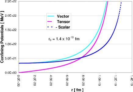
Figure 1: Confining potentials for a $u$ or $d$ quark

Clearly, the vector and tensor potentials are more singular than the scalar one. In Fig. 2 we show the resulting wave functions, Eqs.(113-116), normalized over the interval $[0,r_{0}]$.

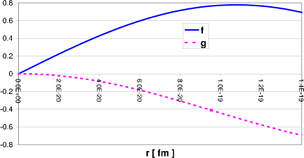
Figure 2: Quark wave functions

These wave functions (in different units) also appear in the phenomenological MIT quark bag model paper5 , where they describe the wave functions of the three quarks in a nucleon. Hence, the current theory shows how such a bag model could possibly originate from fundamental QFT considerations, although the restriction of our theory to single-particle states forbids a direct application of our theory. Obviously, the context is also entirely different as the size of an MIT bag is about $1$ fm, while our single quark bag has Planck length dimensions.

We derived the solutions for a zero bare quark mass. If we introduce a non-zero Higgs field the mass $M$ in the Dirac equation could be non-zero. In this case we find that $V_{s}^{eff}$ is no longer zero but becomes $V_{s}^{eff}=-(32/23)M$. Hence the addition of a bare quark mass $M$ leads to a solution with an apparent mass of $M-(32/23)M=-(9/23)M$. This is an illustration of the importance of self-consistency in these bound-state QFT solutions, and shows that any perturbative considerations may fail, since they even would suggest the wrong sign of the mass. It shows that the calculation of quark solutions for non-zero Higgs fields is feasible, although they have important further consequences, such as additional terms in the total energy expression.

The solutions obtained in this section also have to satisfy additional consistency constraints. If we describe an isolated quark by the state $\left|b^{\dagger}_{\alpha}\right|0\rangle$, then its isospin, color and spin are specified by the index $\alpha$. However, these properties can also be defined as expectation values and expressed as volume integrals over the quantum fields. Naturally, the two possibilities should yield the same answer. For isospin this condition is trivially satisfied, however, for spin and color things are more complicated. These conditions will be discussed in Section VIII. Our $\textrm{O}(\alpha_{s}^{0})$ solution for $\beta=-2/3$ satisfies the resulting conditions exactly. Hence,we have found an exact solution of the equations of motion for $\alpha_{s}=0$. From the analysis of scattering problems we know that QCD is an asymptotically free theory. Hence, it may be quite reasonable to set $\alpha_{s}=0$ at the Planck scale. Since this is the scale that seems to be relevant for the light quarks (see Section IX) the $\alpha_{s}=0$-case might a complete description of dressed quarks in the QCD context. However, in order to describe the mass splitting between the quarks of different charge we need to introduce QED. This theory is not asymptotically free, so that we cannot ignore this coupling and have to apply a perturbative approach in terms of non-zero coupling constants at the Planck scale, anyway. If we assume that $\alpha_{s}\neq 0$, then we have to consider higher order corrections, as well and impose the boundary conditions discussed in VIII. The color condition is the most stringent one and leads to three separate conditions in $\textrm{O}(\alpha_{s})$. Hence, it effectively fixes the integration constants $\nu$ and $\omega$, while putting indirect conditions on $\lambda_{0}$, which in turn leads to $\textrm{O}(\alpha_{s})$ corrections to the value of the radius $x_{0}$. The value of $\mu$ is essentially fixed by the spin condition. Values for $\nu$ and $\omega$ for the bag solution are given in the next sectionVIII. In that section we will also derive the formula for the total (internal) energy of a quark system. The zeroth order result will turn out to be negative. This presents a serious problem if we want to identify this energy with the effective mass of the dressed quark. However, there are various reasons why the model cannot be complete. In the absence of the Higgs field there is no scale parameter in QCD, hence the scale of the quark system is undetermined and it is a mystery how the small quark mass of the light quarks can be reconciled with the effective pointlike nature of the quarks. In Section IX we suggest a novel way to complete the model of single quarks leading to a solution of these interconnected problems.

VIII Observables and conserved quantities

The symmetries of QFT determine the conserved quantities and observables. The invariance under phase transformations of the quark field operator leads to current conservation (cf. Eq.(98)). This relation implies the conservation of baryon number $B$:

$$B=\frac{1}{3}\int d^{3}x\left\langle B_{\alpha}\right|\bar{\psi}\gamma_{0}\psi\left|B_{\alpha}\right\rangle,$$ (117)

where the state vector is either a quark:

$$\left|B_{\alpha}\right\rangle=b_{\alpha}^{\dagger}\left|0\right\rangle,$$ (118)

or an anti-quark:

$$\left|B_{\alpha}\right\rangle=d_{\alpha}^{\dagger}\left|0\right\rangle.$$ (119)

The normalization in Eq.(117) is chosen in such a way that the quark has baryon number $1/3$, and the anti-quark $-1/3$. Notice that we need the $\mathbb{R}$-product to obtain the latter result.

The invariance under translations leads to the canonical energy-momentum tensor:

$$T^{\mu\nu}=\frac{\partial\mathcal{L}}{\partial\frac{\partial\psi}{\partial x^{\nu}}}\frac{\partial\psi}{\partial x_{\mu}}+\frac{\partial\mathcal{L}}{\partial\frac{\partial A_{a}^{\varrho}}{\partial x^{\nu}}}\frac{\partial A_{a}^{\varrho}}{\partial x_{\mu}}-\mathcal{L}g^{\mu\nu}.$$ (120)

By adding a complete differential one can re-express this as the Gauge invariant expression (Peskin ):

$$\Theta^{\mu\nu}=-\mathcal{L}g^{\mu\nu}+\bar{\psi}\textrm{i}\gamma^{\nu}D^{\mu}\psi-F_{a}^{\nu\rho}F_{a,\rho}^{\mu},$$ (121)

where:

$$\partial_{\nu}T^{\mu\nu}=\partial_{\nu}\Theta^{\mu\nu}=0,$$ (122)

so that the spatial integrals of $\Theta^{\mu 0}$ are conserved quantities, corresponding to total energy for $\mu=0$ and total momentum for $\mu=i$. It is easy to quantize Eq.(121) by taking $A_{a}^{\mu}$ outside the quark current, symmetrizing the gluon term, and introducing the $\mathbb{R}$-product.

The spin of the quark is related to the tensor:

$$\tilde{M}^{\mu\nu\rho}=M^{\mu\nu\rho}+\partial_{\alpha}\left[x^{\mu}\left(F_{a}^{\rho\alpha}A_{a}^{\nu}\right)-x^{\nu}\left(F_{a}^{\rho\alpha}A_{a}^{\mu}\right)\right]$$

$$+F_{a}^{\mu\rho}A_{a}^{\nu}-F_{a}^{\nu\rho}A_{a}^{\mu},$$ (123)

where

$$M^{\mu\nu\rho}=x^{\mu}T^{\nu\rho}-x^{\nu}T^{\mu\rho}+\frac{\textrm{i}}{4}\bar{\psi}\gamma^{\rho}\left(\gamma^{\mu}\gamma^{\nu}-\gamma^{\nu}\gamma^{\mu}\right)\psi$$

$$+F_{a}^{\mu\rho}A_{a}^{\nu}-F_{a}^{\nu\rho}A_{a}^{\mu}.$$ (124)

We can show that:

$$\partial_{\rho}\tilde{M}^{\mu\nu\rho}=\partial_{\rho}M^{\mu\nu\rho}=0.$$ (125)

The spin of the quark can now be expressed by the following matrix element:

$$(S_{k})_{\alpha\beta}=\frac{1}{2}\epsilon_{ijk}\int d^{3}r\left\langle B_{\alpha}\right|\tilde{M}^{ij0}\left|B_{\alpha}\right\rangle.$$ (126)

The calculated expectation value should equal $1/2$ in units $\hbar$.

We now express the conserved quantities in terms of the gluon profile functions and the quark wave functions or source functions. From Eq.(121) we get for the total internal energy of the quark system:

$$E_{int}=\int d^{3}r\left\langle B_{\alpha}\right|\Theta^{00}\left|B_{\alpha}\right\rangle=E-\frac{16}{9}E+\frac{16}{3\alpha_{s}}\int_{0}^{r_{0}}drI(r)$$ (127)

where $r_{0}$ is the radius of the quark system and $I(r)$ is given by:

$$I(r)=S_{0}F_{3}-S_{1}\tilde{F}_{0}+\frac{1}{2}r^{2}\left[\left(\frac{F_{3}}{r}\right)^{\prime}+\frac{3}{r^{2}}\tilde{F}_{0}K\right]^{2}$$

$$-\frac{1}{2}r^{2}\left[\left(\frac{\tilde{F}_{0}}{r}\right)^{\prime}+\frac{3}{r^{2}}F_{3}K\right]^{2}-\frac{9}{r^{2}}\left(F_{1}F_{3}-\tilde{F}_{0}F_{4}\right)^{2}$$

$$+\frac{1}{2r^{2}}\left(3F_{1}^{2}-3F_{4}^{2}+\frac{1}{3}\right)^{2}$$

$$+\frac{1}{r^{2}}\left(rF_{4}^{\prime}+3F_{1}K\right)^{2}-\frac{1}{r^{2}}\left(rF_{1}^{\prime}+3F_{4}K\right)^{2}.$$ (128)

After reduction this expression simplifies:

$$I(r)=\hat{S}_{0}\hat{F}_{3}-\hat{S}_{1}\hat{\tilde{F}}_{0}+\frac{1}{2}r^{2}\left[\left(\frac{\hat{F}_{3}}{r}\right)^{\prime}\right]^{2}$$

$$-\frac{1}{2}r^{2}\left[\left(\frac{\hat{\tilde{F}}_{0}}{r}\right)^{\prime}\right]^{2}-\frac{9}{r^{2}}\left(\hat{F}_{1}\hat{F}_{3}-\hat{\tilde{F}}_{0}\hat{F}_{4}\right)^{2}$$

$$+\frac{1}{2r^{2}}\left(3\hat{F}_{1}^{2}-3\hat{F}_{4}^{2}+\frac{1}{3}\right)^{2}+\hat{F}_{4}^{\prime 2}-\hat{F}_{1}^{\prime 2}.$$ (129)

The internal energy of the system is now expressed completely in terms of reduced profile functions and therefore is finite even if the original profile functions are singular. For the $\rm O(\alpha_{s}^{0})$ bag solution with $\beta=-2/3$ we get $E_{int}=E-(32/9)E<0$. In Section IX we will address the problem associated with the negative character of this internal energy.

The total momentum of the system is easily calculated and equals zero, as expected:

$$P^{i}_{tot}=\int d^{3}r\left\langle B_{\alpha}\right|\Theta^{i0}\left|B_{\alpha}\right\rangle=0.$$ (130)

Since we are considering a system in isolation, it would not make sense to assign a momentum to it. Its momentum only becomes relevant when we embed it in ordinary QFT and the quark interacts with other particles.

Let us now consider the spin. We obtain:

$$(S_{k})_{\alpha\beta}=(\sigma_{k})_{\alpha\beta}\left\{\frac{1}{2}-\frac{32}{9\alpha_{s}}\int_{0}^{r_{0}}drr\left(S_{0}F-S_{1}F_{1}\right)\right.$$

$$-\frac{32}{9\alpha_{s}}\int_{0}^{r_{0}}\frac{dr}{r}\left(rF_{3}^{\prime}-F_{3}+2\tilde{F}_{0}K\right)\left(rF_{4}^{\prime}+2{F}_{1}K\right)$$

$$+\left.\frac{32}{9\alpha_{s}}\int_{0}^{r_{0}}\frac{dr}{r}\left(r\tilde{F}_{0}^{\prime}-\tilde{F}_{0}+2F_{3}K\right)\left(rF_{1}^{\prime}+2{F}_{4}K\right)\right\}.$$ (131)

The first term already provides the exact answer, hence the remaining terms should add up to zero. After reduction we can convert this to the condition:

$$\frac{16}{27}=-\frac{32}{9\alpha_{s}}\left[\int_{0}^{r_{0}}drr\left(\hat{S}_{0}\hat{F}_{4}-\hat{S}_{1}\hat{F}_{1}\right)\right.$$

$$-\left.\int_{0}^{r_{0}}dr\left\{\left(r\hat{F}_{3}^{\prime}-\hat{F}_{3}\right)\hat{F}_{4}^{\prime}-\left(r\hat{\tilde{F}}_{0}^{\prime}-\hat{\tilde{F}}_{0}\right)\hat{F}_{1}^{\prime}\right\}\right],$$ (132)

or after integration by parts:

$$r_{0}^{2}\left.\left[\left(\frac{\hat{X}}{r}\right)^{\prime}\hat{V}+\left(\frac{\hat{Y}}{r}\right)^{\prime}\hat{U}\right]\right|^{r_{0}}=-\frac{\alpha_{s}}{3}.$$ (133)

To $\rm O(\alpha_{s}^{0})$ this equation is automatically satisfied by the solutions $\hat{X}(r)=\hat{Y}(r)=\beta Er$, e.g. by the bag solution with $\beta=-2/3$. Its satisfaction for this bag solution can also be related to the identity $\hat{S}_{0}=S_{0}$, which guarantees the validity of Eq. (VIII) to lowest order. The condition (133) can assist in fixing the four free parameters defined in the perturbative scheme in Section V.

There is another conserved quantity for single quarks, namely color. The reason that this is not usually seen as an observable, is because quarks are usually not considered in isolation (physically they only appear in color singlets). However, since we are considering single quark solutions to the field equations, we clearly have to examine this property as well. Color is associated with the invariance of QCD under local gauge transformations. The relevant infinitesimal transformations are paper6 :

$$\psi\rightarrow\psi^{\prime}=\psi-\textrm{i}\frac{\epsilon}{2}\boldsymbol{\omega}\bullet\boldsymbol{\lambda}\psi$$ (134)

and

$$\textbf{A}_{\mu}\rightarrow\textbf{A}_{\mu}^{\prime}=\textbf{A}_{\mu}-\epsilon\textbf{A}_{\mu}\boldsymbol{\times}\boldsymbol{\omega}-\frac{\epsilon}{g_{s}}\partial_{\mu}\boldsymbol{\omega}.$$ (135)

The current corresponding to this transformation is given by:

$$\textbf{C}^{\mu}=\frac{1}{2}\bar{\psi}\gamma^{\mu}\boldsymbol{\lambda}\psi+\frac{1}{2}\textbf{F}^{\mu\nu}\boldsymbol{\times}\textbf{A}_{\nu}-\frac{1}{2}\textbf{A}_{\nu}\boldsymbol{\times}\textbf{F}^{\mu\nu}.$$ (136)

Since

$$\textbf{C}^{\mu}=g_{s}^{-1}\partial_{\nu}\textbf{F}^{\mu\nu},$$ (137)

it follows immediately that:

$$\partial_{\mu}\textbf{C}^{\mu}=0.$$ (138)

Hence, we can define the conserved color density ($\mu=0$):

$$\left\langle C_{k}^{0}\right\rangle_{\alpha\beta}=\left\langle B_{\alpha}\right|\int d^{3}x\left[\bar{\psi}\gamma^{0}\frac{\lambda_{k}}{2}\psi\right.$$

$$+\left.\frac{1}{2}\left(\textbf{F}^{0\nu}\boldsymbol{\times}\textbf{A}_{\nu}-\textbf{A}_{\nu}\boldsymbol{\times}\textbf{F}^{0\nu}\right)_{k}\right]\left|B_{\beta}\right\rangle.$$ (139)

The first term in the right-hand side of Eq.(VIII) equals the bare color, so that we have to demand that the remaining terms yield zero. Since this leads to a constraint on an integral, this condition is not easy to implement. A simpler condition arises if we use the identity, Eq.(137), again. This leads to the condition:

$$\left\langle C_{k}^{0}\right\rangle_{\alpha\beta}=\frac{1}{g_{s}}\left\langle B_{\alpha}\right|\int d^{3}x\partial_{\nu}F_{k}^{0\nu}\left|B_{\beta}\right\rangle$$

$$=\frac{1}{g_{s}}\left\langle B_{\alpha}\right|\int dSF_{k}^{0n}\left|B_{\beta}\right\rangle=\left\langle\alpha\right|\frac{\lambda_{k}}{2}\left|\beta\right\rangle.$$ (140)

Writing this out in profile functions, we obtain:

$$\left.r_{0}^{2}\left[\left(\frac{F_{3}}{r}\right)^{\prime}+\frac{3}{r^{2}}\tilde{F}_{0}K\right]\right|_{r_{0}}=\frac{\alpha_{s}}{2},$$ (141)

where $r_{0}$ is the radius of the quark bag for the bag solution. After reduction this condition can be written as:

$$\left.r_{0}^{2}\left[\left(\frac{\hat{X}}{r}\right)^{\prime}\hat{E}+\left(\frac{\hat{Y}}{r}\right)^{\prime}\hat{E}^{-1}\right]\right|^{r_{0}}=\alpha_{s}.$$ (142)

Notice the similarity with the spin condition Eq. (133). As for the spin case, this condition is automatically satisfied for the $\textrm{O}(\alpha_{s}^{0})$ solutions Eq.(69). We can combine the color and spin condition to formulate the following boundary conditions:

$$\left(\frac{\hat{Y}}{r}\right)^{\prime}=-\frac{\alpha_{s}}{r_{0}^{2}}\hat{E}\frac{1/3+\hat{E}^{-1}\hat{V}}{\hat{U}\hat{E}-\hat{E}^{-1}\hat{V}},~{}~{}~{}~{}~{}~{}~{}~{}r\rightarrow r_{0}$$

$$\left(\frac{\hat{X}}{r}\right)^{\prime}=\frac{\alpha_{s}}{r_{0}^{2}}\hat{E}^{-1}\frac{1/3+\hat{E}\hat{U}}{\hat{U}\hat{E}-\hat{E}^{-1}\hat{V}},~{}~{}~{}~{}~{}~{}~{}~{}r\rightarrow r_{0}.$$ (143)

Since either $\hat{E}$ or $\hat{E}$ is singular at $r=r_{0}$, we need to treat these boundary conditions as limiting processes, rather than as point identities. For the bag solution we have:

$$\hat{E}=\frac{1}{(x-x_{0})^{2}}\tan^{2}x_{0}$$ (144)

near the surface $x=x_{0}$. After expanding $\hat{X}$ in a Taylor expansion for $r\rightarrow r_{0}$, we then arrive at three conditions, which allow us to fix the perturbative parameters $\nu$ and $\omega$. Numerically, we find:

$$\nu=-0.052\alpha_{s}~{}~{}~{}\omega=1.092\alpha_{s}.$$ (145)

The third condition is more tricky as it involves an adjustment of the radius of the quark bag. A rough calculation indicates that we have to adjust $x_{0}$ from $2.043$ to $2.129$, however, a more complete numerical study is required to get precise answers.

In this section we considered the observables which play the role of boundary conditions in our formulation. Other observables, such as the magnetic moment, arise from the interactions with external fields, and must be calculated with standard perturbative methods. Clearly, our formulation has little to add to such calculations except perhaps providing physical cut-off parameters in view of the finite size of the dressed quarks.

IX The role of general relativity and the determination of the mass of the light quarks

As seen in the previous section, the total QFT energy of the dressed quark system is negative. Within the context of QFT there is only one obvious contribution which could compensate for this negative energy and that is the Higgs field. We expect that the two finite real Higgs solutions, whose classical approximations could be characterized by the values $\phi=\pm\surd{\mu^{2}/\lambda}$, would have such an effect and lead to an overall positive energy, which can be associated with the mass of the quarks. However, to enable this treatment, one needs to know the exact nature of the Higgs Lagrangian at the fundamental level and preferably its relationship to the massive vector bosons. These Higgs terms would add an additional set of equations and profile functions and therefore add considerably complexity. It therefore seems more natural to look initially at the trivial Higgs sector with a zero Higgs field. Strictly speaking, this ”trivial” Higgs sector is not completely zero, as the quark source term would induce a final Higgs field even if we choose the small Higgs solution in the cubic field equation. However, we believe that it would be a fairly good approximation to approximate this lower branch by a zero Higgs field. The consequence of this assumption is that we need to find other solutions for the following two problems (1) The absence of a scale defining parameter; (2) The negative energy of the system. A system with negative energy and unconstrained scale would contract without bound in order to minimize its energy, unless its scale is fixed, which it is not in QCD. To prevent this collapse we consider the consequences of general relativity (GR). When the energy approaches the Planck scale, the effects of GR become important, and the large magnitude of the negative internal energy will halt the implosion. To treat these GR effects in a QFT context is non-trivial, and brings us in uncharted territory. However, by treating these effects perturbatively, we avoid some of the tricky problems. Since this inclusion of the effects of GR, in combination with the vacuum energy, leads to a spectacular agreement with experiment, we feel that there is good evidence for the validity of this perturbative approach.

The effect of GR can be represented through the metric tensor, whose spatial component $\sqrt{{}^{3}g}$ modifies the spatial energy integral:

$$E_{int}=\int d^{3}x~{}\Theta_{0}^{~{}0}\rightarrow\int d^{3}x\sqrt{{}^{3}g}~{}\Theta_{0}^{~{}0},$$ (146)

where the energy density is represented by the component $\Theta_{0}^{~{}0}$ (depending on the metric convention, we may also need an additional minus sign). The spatial metric ${}^{3}g$ is controlled by the local energy density inside the quark. The simplest approximation is to replace this energy distribution by an effective mass $M_{eff}$ at the origin, with $M_{eff}$ equalling the total internal energy $-(23/9)E$. By expanding the resulting integral in $G$ we obtain a well-defined integral:

$$E_{int}\approx\int d^{3}x\left(1+\frac{2M_{eff}\,G}{r}\right)^{3/2}~{}\Theta_{0}^{~{}0}$$

$$\approx\int d^{3}x\left(1-3\frac{\gamma GE}{r}\right)~{}\Theta_{0}^{~{}0},$$ (147)

where $\gamma=23/9$. At the end of this section we will also discuss results where the point mass at the center is replaced by an integrated density distribution based on the internal quark wave functions $f$ and $g$. Carrying out the integral we obtain approximately:

$$E_{int}\approx-\gamma\,E\left(1-\frac{3\gamma GE^{2}}{\delta x_{0}}\right),$$ (148)

where we replaced $1/r$ by its expectation value $\left\langle 1/r\right\rangle=E/\delta x_{0}$ where $\delta=0.6019\cdots$ for the bag wave function. This expression reaches its minimum for

$$E=\sqrt{\frac{\delta x_{0}}{9\gamma G}}~{}\rightarrow~{}r_{0}=\sqrt{\frac{9x_{0}\gamma G}{\delta}}.$$ (149)

The correction $3\gamma GE^{2}/\delta x_{0}$ to the Minkowski metric equals $1/3$, which means that the first order (perturbative) usage of GR is consistent. Both the radius $r_{0}$ and the internal frequency $E$ are of Planck scale, with $r_{0}=8.8\,\,\textrm{l}_{\textrm{Planck}}=1.4\times 10^{-19}\textrm{fm}$ and $E=0.23\,\textrm{M}_{\textrm{Planck}}=2.8\times 10^{21}\textrm{MeV}$. The negativity of the internal quark energy was essential for the stabilization of the system. Hence, a property that appeared like a serious problem of the model actually was necessary to stabilize the system and to fix the scale. However, the relationship between the negative internal energy of Planck mass magnitude and the quark mass, which is positive and lies in the MeV range, is still unexplained.

In order to address this problem we introduce the vacuum energy density $\epsilon$, or what is equivalent a finite cosmological constant. Recently, a cosmological model was developed which is based on the presence of this vacuum (dark) energy Greben10 . The associated non-perturbative metric of the vacuum universe has a very simple time dependence:

$$g_{\mu\nu}=\eta_{\mu\nu}g(t)=\eta_{\mu\nu}(t_{s}/t)^{2},$$ (150)

where the characteristic time $t_{s}$ follows from the postulated vacuum energy density $\epsilon$: $t_{s}=(3/8\pi G\epsilon)^{1/2}$. Another consequence of this cosmological model is that $t_{s}=1/H_{0}$, where $H_{0}$ is the Hubble constant, while $t_{s}$ also represents the age of the universe as measured by a co-moving observer. Fitting recent supernovae data one arrives at a vacuum energy density of $\epsilon=3.97\times 10^{-47}~{}\textrm{GeV}^{4}$ and an age of the universe of $t_{s}=13.8$ billion years. The vacuum metric leads to the effective time-dependent vacuum energy density:

$$\epsilon_{eff}(t)=\sqrt{{}^{3}g(t)}~{}\epsilon=(t_{s}/t)^{3}~{}\epsilon.$$ (151)

We now make the novel assumption that the creation of a quark is associated with the creation of a small vacuum universe (a small big bang). The creation of this bag terminates at a time $t_{c}$, when the size of the bag matches the size $r_{0}$ of the QFT quark bag. Since this creation time $t_{c}$ is very small, the effective vacuum energy density is very large (just like it was $t_{c}$ seconds after the big bang), and the resulting energy can potentially cancel the internal energy, leaving a net quark mass of much smaller magnitude. According to the Heisenberg uncertainty relation Briggs the total energy during this time interval $t_{c}$ is uncertain by an amount $\hbar/2t_{c}$, so that it is possible during this time interval to create a mass of magnitude $\hbar/2t_{c}$. Hence, we set:

$$m_{q}\,=\frac{\hbar}{2}\frac{1}{t_{c}},$$ (152)

and verify whether this assumption for the quark mass is consistent with the energy balance:

$$m_{q}=\frac{\hbar}{2}\frac{1}{t_{c}}=E_{vacuum}+E_{int},$$ (153)

where $E_{int}$ is the minimum energy determined earlier. Since the quark mass will turn out to be infinitesimal compared to the other terms, it is natural to ignore the left-hand term:

$$E_{vacuum}+E_{int}=\frac{4\pi}{3}\left(\frac{x_{0}}{E}\right)^{3}\epsilon\left(\frac{t_{s}}{t_{c}}\right)^{3}+E_{int}\approx 0.$$ (154)

Clearly, the required cancelation between internal and vacuum energy can only happen if the internal QFT energy is negative, so the negativity of the internal energy is again essential for the construction of a realistic quark model. The cancelation condition leads to a creation time $t_{c}$:

$$t_{c}=\left(\frac{4\pi x_{0}}{2\gamma}\right)^{1/3}\left(\frac{3}{8\pi}\right)^{1/2}\left(\frac{G}{\epsilon}\right)^{1/6}\left(\frac{9\gamma}{\delta}\right)^{2/3}.$$ (155)

This expresses the creation time - and therefore the mass of the quark - exclusively in terms of the cosmological parameters $G$ and $\epsilon$ (or $H_{0}$), as the remaining parameters ($x_{0}=2.0478\cdots,\gamma=23/9~{}\mathrm{and}~{}\delta\approx.60$) are fixed by the formalism. We obtain $t_{c}=1.04\times 10^{-22}$ s. According to Eq.(152) this corresponds to a mass of the dressed quark of $m_{q}=3.17$ MeV, confirming the smallness of this mass in comparison to the Planck scale. Expanding the integral in Eq.(IX) to $\textrm{O}(G^{2})$ only gives a small correction: one finds $m_{q}=3.50$ MeV (since there are other terms contributing in $\textrm{O}(G^{2})$ which are not examined, we do not claim that this result is more accurate than the first order result). Replacing the mass term $M/r$ in the metric factor by a continuous distribution based on the internal quark wave functions one finds $m_{q}=4.05$ MeV. These three results give a good indication of the uncertainty in the result $m_{q}=3.17$ MeV, due to the uncertainties in unifying QCD and GR. Let us now compare this result to ”experiment”.

Reference Review06 quotes the following lattice values for the average up and down mass: $3.8\pm 0.8$ MeV, while the average value excluding the lattice is quoted as: $4.4\pm 1.5$ MeV. Very recently Davies et. al.Davies reported on a new determination of the light quark masses of much higher precision. They quote the following average values for the light quark masses: $m_{q}(2~{}\textrm{GeV})=3.40\pm.07$ MeV and $m_{q}(3~{}\textrm{GeV})=3.07\pm.06$ MeV, where the energy in brackets is the scale used in their calculation. The agreement between our result $3.17$ MeV and these ”experimental” values is extremely good, especially if one takes into consideration the enormous differences between the particle physics scale and the cosmological scale, from which our masses have been derived. Naturally, additional effects, like the electro-weak forces (which splits the degeneracy between u and d-quarks) and $\textrm{O}(\alpha_{s})$-terms (if $\alpha_{s}\neq 0$), have to be included in more detailed calculations. However, the current level of agreement with experiment is clearly a strong endorsement of the theory presented here and confirms that this solution corresponds to the first generation of quarks.

X Summary and Discussion

In this paper we formulate a new set of methods in QFT that can be used to describe the internal properties and masses of elementary particles. The exact non-perturbative operator structure of the fermion and boson quantum fields is constructed by demanding the satisfaction of the full set of coupled quantum field equations. Starting from the basic QCD Lagrangian with bare pointlike massless quarks, we derive the internal wave functions of the dressed quarks and the form of the binding potentials. The binding mechanism of the localized quark-gluon state is topological in nature as it enabled by the non-linear structure of the equations and is independent of the magnitude of the strong coupling constant. Since all equations and fields refer to a single space-time coordinate, an additional operator prescription is required to reflect the opposite ordering of particles and anti-particles. This prescription (the so-called $\mathbb{R}$-product) also resolves the so-called cosmological constant problem, as it leads to a more fundamental and less ambiguous definition of the vacuum in QFT.

The calculation of the quark mass is complicated by the fact that the QFT expectation value of the energy operator is negative. It is possible that by including an elementary Higgs-quark interaction, this problem may be resolved, however, this can only account for two of the three quark generations. The third - and probably basic - generation would then correspond to the trivial (zero) Higgs solution. However, in the absence of a Higgs field we need another entity to counter the negative QFT energy and give the system a scale. We propose a novel solution for this puzzle by involving the perturbative use of gravitational forces at the Planck scale. In this way we arrive at a positive mass which is amazingly close to accepted phenomenological values for the light quarks.

The current theory would get further support if we can deduce the existence of the two higher generations of quarks. However, as we indicated above, this may well require the inclusion of a Higgs quark interaction, which will entail more profile functions and a more involved formulation. But it also offers a chance to verify various models of this force and the associated electro-weak interaction at a more fundamental level than the standard model, by comparing the predictions to experiment. Affirmation of the proposed Lagrangians would undoubtedly lead to a more unified picture of Nature. Another, desirable extension is the perturbative inclusion of QED to explain the mass differences between quarks within one generation. Clearly, QCD cannot describe the dressing of leptons, so that for this sector the non-linear electro-weak interaction must induce the binding mechanism. The application of our formulation to unbroken SU(2) is fairly straightforward (for example we already found that the factor 32/9 is replaced by 3/2), but the chiral nature of the electro-weak interaction is more difficult to include. Again, this application to leptons offers a good opportunity to test various models of the electro-weak interactions at the fundamental level, as it is possible that the complicated multiplet structure in the standard model is absent at a more fundamental level. The smallness of the neutrino masses would put extremely strong constraints on the possible theories, and if a model was successful in predicting the lepton masses then it would mark a historic breakthrough in our understanding of Nature.

The application of the new methodology is not completely limited to the description of the internal dynamics of elementary particles. It can also be used to construct free boson propagators using the new quantization method for solving the (homogeneous) equations of motion. The $\mathbb{R}$-product also could play a role in scattering diagrams if there are non-linear vertices with common space-time coordinates (as pointed out repeatedly, the $\mathbb{R}$-product does not affect the algebra of operators defined for different space-time coordinates). In scattering calculations the finite size of dressed fermions (emerging from the current theory) could also play a role in defining physical cut-offs, and thereby ensure the finiteness of otherwise infinite diagrams. However, the size of the light quarks (about 8 Planck lengths) is beyond measurement. If the higher generations of quarks are indeed due to coupling to an elementary Higgs field, then their sizes would be substantially larger, and of the order of 0.004 fm on average, so they might be measurable. Outside of these specific effects, the standard scattering formulation would remain unaltered, and so all the successful scattering applications of the standard model seem fully consistent with the current generalizations of QFT.

Appendix A The $\mathbb{R}$-product

The formulation of QFT contains an inherent asymmetry between particles and anti-particles, which reflects the inadequacy of the mathematical language in which we express this formulation. Since we are constrained by this language we have to add another rule to QFT, which together with the usual rules constitutes a symmetric representation of the world of particles and anti-particles. In this appendix we define this rule. It should form an inherent part of the foundations of QFT. Its absence in the current practice of QFT has led to many misconceptions and is also responsible for the so-called cosmological constant problem, which constitutes the biggest discrepancy ever between theory and experiment in the history of physics.

Consider a typical operator expression in QFT:$\bar{\psi}O\psi$. If we evaluate the vacuum matrix element of this operator and concentrate on the particle contributions we get:

$$<0|\bar{\psi}O\psi|0>=\sum_{\alpha,\beta}<0|b^{\dagger}_{\alpha}b_{\beta}|0>(\bar{\phi}_{\alpha}O\phi_{\beta})=0,$$ (156)

as expected. If we look at the expectation value for a particle state we get:

$$<0|b_{\gamma}|\bar{\psi}O\psi|b^{\dagger}_{\gamma}|0>=(\bar{\phi}_{\gamma}O\phi_{\gamma}),$$ (157)

expressing the desired link between the state considered and the matrix element. However, when we consider the anti-particle contribution of the operator we have:

$$<0|\bar{\psi}O\psi|0>=\sum_{\alpha,\beta}<0|d_{\alpha}d^{\dagger}_{\beta}|0>(\bar{\phi}_{\alpha}^{a}O\phi_{\beta}^{a})$$

$$=\sum_{\alpha}(\bar{\phi}_{\alpha}^{a}O\phi_{\alpha}^{a}),$$ (158)

which is in general non-zero, and can even be infinite, as the sum is unrestricted. Clearly, this asymmetry is unacceptable and illustrates the incompleteness of the standard QFT description (notice that there is no problem with mixed terms such as $b_{\alpha}^{\dagger}d_{\beta}^{\dagger}$, which are responsible for the quantum fluctuations). The origin of this asymmetry between particles and anti-particles is that the right-hand operator $\psi$ contains particle annihilation operators and anti-particle creation operators. This particular combination is required by baryon (or lepton) number conservation. However, it leads to the possibility of creating anti-particles - and the impossibility to create particles - when operating with $\psi$ on the ket-vector, even if it is vacuum state. Similarly, the operator on the left, $\bar{\psi}$, contains a combination of particle creation and anti-particle annihilation operators, again required by baryon number conservation. This combination displays a similar unacceptable asymmetry when operating to the left on a bra-vector. Let us see how we can restore the symmetry between particles and anti-particles.

To eliminate vacuum terms, like those in Eq.(A), one usually applies the normal product to the bilinear expression:

$$d_{\alpha}d_{\beta}^{\dagger}\rightarrow:d_{\alpha}d_{\beta}^{\dagger}:=-d_{\beta}^{\dagger}d_{\alpha}.$$ (159)

Clearly, the anti-particle contributions to the vacuum matrix element now also vanish. The usual justification for this heuristic procedure in QFT is that in QFT one is not interested in absolute energies, but rather in relative energies, such as excitation energies. By consistently replacing bilinear expressions by the normal product, one then eliminates such sources of infinities from the start. However, within GR energy leads to a modification of the metric, so that one cannot arbitrarily rescale the energy. Thus the heuristic replacement of bilinear expressions by their normal product is no longer seen as acceptable. This has led to the consideration of QFT vacuum contributions to the energy as a real phenomenon (especially in cosmology), although this is in total disagreement with experimental observations. As we saw above, the normal product is needed to restore the symmetry between particles and anti-particles, so we cannot simply dismiss it because it is a heuristic trick. Rather, we have to explain the origin of this heuristic prescription and should definitely not accept the reality of the vacuum contributions as a fait accompli, especially since these contributions are associated with an unacceptable asymmetry between particles and anti-particles and are in strong disagreement with observation.

The key towards the solution of this problem is to examine the normal product from a different perspective. The normal product is defined as a rearrangement of the operators, so that the creation operators are shifted to the left of the annihilation operators. The normal product is also widely used in the derivations of the scattering expansion in QFT, although there it is used as a convenient mathematical construct and not employed heuristically. In its current heuristic application, Eq.(159), it is equivalent to the inversion of the order of the anti-particle operators, as the normal product leaves the particle operators unaffected in the QFT expression $\bar{\psi}O\psi$ as $:b^{\dagger}_{\alpha}b_{\beta}:=b^{\dagger}_{\alpha}b_{\beta}$. Hence, an equivalent definition of the normal product for the relevant QFT expressions is that the order of the anti-particle operators must be reversed. We will refer to this re-ordering as the $\mathbb{R}$-product. We will argue that there is a fundamental theoretical justification for this product, which is lacking in the heuristic application of the normal product. Hence, in the bilinear expressions considered one can justify the use of the normal product indirectly via the justification for the $\mathbb{R}$-product. For longer expressions the usage of the $\mathbb{R}$-product, rather than the normal product, leads to different results. However, most of the long expressions involve different space-time coordinates, where neither the $\mathbb{R}$-product, nor the heuristic normal product applies. If we analyze the usage of the heuristic application of the normal product in the existing QFT literature, we see that it is customary to define the (interaction) Hamiltonian heuristically as normal ordered (see e.g. Sakurai ), before it is inserted in the matrix elements of the $S$-matrix expansion. This means that there is no heuristic normal ordering between operators corresponding to different coordinates $x$ and $x^{\prime}$ (it makes no difference if we let $x\rightarrow x^{\prime}$, for the current practice it is only important that the coordinates were different originally). In fact the heuristic usage of normal ordering between different spatial integrals in the $S$-matrix expansion would destroy the whole structure and meaning of the $S$-matrix expansion. Hence, the heuristic use of the normal product must be limited to strings of operators that all belong to a single coordinate $x$ (we will later discuss the fundamental origin of this rule). But for such short expressions, corresponding to a single $x$, the normal product and the $\mathbb{R}$-product are often equivalent, so that either one can be used. This equivalence for the simplest QFT expressions is the likely reason why the $\mathbb{R}$-product has not been discovered before in QFT, as the usage of the normal product was often adequate.

For longer expressions belonging to a single space-time coordinate the usage of the $\mathbb{R}$-product leads to very different results than the normal product, so here it becomes of importance to use the $\mathbb{R}$-product. In the current bound-state application of QFT we encounter many long chains of creation and annihilation operators belonging to a single coordinate $x$, so our transition to the $\mathbb{R}$-product has major consequences for the current formulation (in standard scattering applications of non-Abelian QFT it might also have consequences, as these also involve strings of operators at the same space-time point). Consider a longer local QFT expression, like $d_{\alpha}b_{\beta}b_{\gamma}^{\dagger}d_{\delta}^{\dagger}$ and $b_{\gamma}^{\dagger}d_{\delta}^{\dagger}d_{\alpha}b_{\beta}$(it is essential to use expressions that actually occur in the usage of QFT, since we are trying to correct a defect of QFT that occurs in its actual representation). Using the normal product we get:

$$:d_{\alpha}b_{\beta}b_{\gamma}^{\dagger}d_{\delta}^{\dagger}:=b_{\gamma}^{\dagger}d_{\delta}^{\dagger}d_{\alpha}b_{\beta},$$

$$:b_{\gamma}^{\dagger}d_{\delta}^{\dagger}d_{\alpha}b_{\beta}:=b_{\gamma}^{\dagger}d_{\delta}^{\dagger}d_{\alpha}b_{\beta},$$ (160)

whereas the $\mathbb{R}$-product leads to:

$$\mathbb{R}\left[d_{\alpha}b_{\beta}b_{\gamma}^{\dagger}d_{\delta}^{\dagger}\right]=-b_{\beta}b_{\gamma}^{\dagger}d_{\delta}^{\dagger}d_{\alpha},$$

$$\mathbb{R}\left[b_{\gamma}^{\dagger}d_{\delta}^{\dagger}d_{\alpha}b_{\beta}\right]=-b_{\gamma}^{\dagger}b_{\beta}d_{\alpha}d_{\delta}^{\dagger}.$$ (161)

Under the normal product the distinction between the two initial expressions is lost, while the $\mathbb{R}$-product maintains the integrity of the expression, while still ensuring that the vacuum matrix element vanishes. If we apply the resulting expressions to a one-particle state then we get zero under the normal product, while the $\mathbb{R}$-product gives a finite outcome. Hence, the $\mathbb{R}$-product leads to the survival of non-linear terms in the field equations which are essential for the existence of bound states, such as considered in this paper.

The physical justification of the $\mathbb{R}$-product is that it embodies Feynman’s interpretation of anti-particles as particles moving backward in time. In the $S$-matrix expansion the ordering of operators defined at different times is taken care off by the time-ordering procedures of standard QFT. However, when anti-particles all belong to the same time $t$, this ordering cannot be implemented by explicit time ordering. That is why one has to impose the $\mathbb{R}$-product on local expressions to ensure the correct ordering of interactions and vertices. The terms forward and backward in time may seem a bit inappropriate for local operators defined at a single $t$, so let us analyze this concept in the current context. In the matrix elements the ket-vector is usually seen as the initial state, while the bra-vector is seen as the final state. From this perspective, the operator right-most in a chain first operates on the ket-vector, and is ”earlier” in time than operators further to the left. For a chain of anti-particle operator the left-most operator must first act on the initial state (i.e. the ket vector), etc. This can be accomplished by applying the $\mathbb{R}$-product to expressions dependent on one space-time coordinate.

One consequence of the $\mathbb{R}$-product is that one cannot insert a complete set of states somewhere inside the operator expression. Hence, the manipulation and reduction of an $\mathbb{R}$-product requires special care, as we will also see in the following example. Consider the following reduction:

$$\mathbb{R}\left[b_{\alpha}^{\dagger}d_{\beta}^{\dagger}d_{\gamma}b_{\delta}\right]=-b_{\alpha}^{\dagger}d_{\gamma}d_{\beta}^{\dagger}b_{\delta}=-b_{\alpha}^{\dagger}b_{\delta}\delta_{\gamma\beta}$$

$$+b_{\alpha}^{\dagger}d_{\beta}^{\dagger}d_{\gamma}b_{\delta}=-\delta_{\gamma\beta}\mathbb{R}\left[b_{\alpha}^{\dagger}b_{\delta}\right]-\mathbb{R}\left[b_{\alpha}^{\dagger}d_{\gamma}d_{\beta}^{\dagger}b_{\delta}\right].$$ (162)

We see that if we commute the anti-particle operators under the $\mathbb{R}$-product, we get an extra minus sign in the anti-commutator, compared to the original anti-commutator, Eq.(11). This is conveniently summarized by the following anti-commutation rule:

$$\mathbb{R}\left[\cdots\left\{d_{\alpha}^{\dagger},d_{\beta}\right\}\cdots\right]=\mathbb{R}\left[\cdots(-\delta_{\alpha\beta})\cdots\right],x=x^{\prime},$$ (163)

where $x$ and $x^{\prime}$ are the coordinates belonging to the two anti-particle operators. Since, all operators have to be expressed in $\mathbb{R}$-product form, we have to apply this extra minus sign whenever we contract anti-particle terms corresponding to the same space-time point in the equations of motion or in the expressions for the observables. These minus signs are absolutely necessary for deriving consistent equations, in fact we established the need for these signs, before we had discovered their origin in the $\mathbb{R}$-product. We will see in Appendix B, that the $\mathbb{R}$-product also enables us to derive the general operator solution of the equations of motion by including operator chains of any length in the expressions.

Appendix B General operator solution of the equations of motion

Since we are only interested in the creation and annihilation operator aspects in the current appendix, we will use a simplified, partly symbolic, notation. Consider first the Dirac equation. Writing this in the form:

$$H_{0}\psi=\psi A,$$ (164)

we get a series of one- and many-body terms on the right, when we use the expansions Eq.(8) and (II) for the quark and gluon field operators:

$$H_{0}\psi=\sum_{\alpha,\beta,\gamma}\left[b_{\alpha}\phi_{\alpha}+d_{\alpha}^{\dagger}\phi_{\alpha}^{a}\right]\left[b^{\dagger}_{\beta}b_{\gamma}A_{a,\beta\gamma}^{\mu,pp}\right.$$

$$+\left.d_{\beta}d_{\gamma}^{\dagger}A_{a,\beta\gamma}^{\mu,aa}+b_{\beta}^{\dagger}d_{\gamma}^{\dagger}A_{a,\beta\gamma}^{\mu,pa}+d_{\beta}b_{\gamma}A_{a,\beta\gamma}^{\mu,ap}\right].$$ (165)

After contraction, some of the right-hand terms lead back to the single particle annihilation or anti-particle creation operator. For example,

$$b_{\alpha}b_{\beta}^{\dagger}b_{\gamma}\rightarrow\delta_{\alpha\beta}b_{\gamma};~{}~{}~{}~{}d_{\alpha}^{\dagger}d_{\beta}b_{\gamma}\rightarrow-\delta_{\alpha\beta}b_{\gamma},$$ (166)

where the minus sign arises from the $\mathbb{R}$-product. However, there are also a lot of many-body operators. For example, we have:

$$b_{\alpha}b_{\beta}^{\dagger}b_{\gamma}\rightarrow-b_{\beta}^{\dagger}b_{\alpha}b_{\gamma};~{}~{}~{}~{}d_{\alpha}^{\dagger}d_{\beta}b_{\gamma}\rightarrow-d_{\beta}d_{\alpha}^{\dagger}b_{\gamma}\,,$$ (167)

both of which correspond to many-body terms. Notice that when reducing operator expressions in $\mathbb{R}$-product form, the anti-particle creation operators have to end up towards the right after contraction. After, carrying out the $\mathbb{R}$-product in the final reduced expression, these creation operators will then end up to the left, as desired in reduction processes. This explains why the second term in Eq.(167) must be considered a many-body term.

Writing out Eq.(B) explicitly, we can cast the quark field operator in the following form:

$$\psi=\sum_{\alpha}b_{\alpha}\phi_{\alpha}+\sum_{\alpha}d_{\alpha}^{\dagger}\phi_{\alpha}^{a}+\sum_{\alpha,\beta,\gamma}\left[b_{\alpha}^{\dagger}b_{\beta}b_{\gamma}\phi_{\alpha\beta\gamma}^{ppp}\right.$$

$$+b_{\alpha}d_{\beta}d_{\gamma}^{\dagger}\phi_{\alpha\beta\gamma}^{paa}+b_{\alpha}^{\dagger}b_{\beta}d_{\gamma}^{\dagger}\phi_{\alpha\beta\gamma}^{ppa}+b_{\alpha}d_{\beta}b_{\gamma}^{\dagger}\phi_{\alpha\beta\gamma}^{pap}$$

$$+\left.d_{\alpha}d_{\beta}^{\dagger}d_{\gamma}^{\dagger}\phi_{\alpha\beta\gamma}^{aaa}+d_{\alpha}^{\dagger}b_{\beta}^{\dagger}d_{\gamma}^{\dagger}\phi_{\alpha\beta\gamma}^{apa}\right].$$ (168)

The reason that we have $6$ many-body terms instead of the expected $4\times 2=8$, is that two terms, namely $b_{\alpha}^{\dagger}b_{\beta}d_{\gamma}^{\dagger}$ and $b_{\alpha}d_{\beta}d_{\gamma}^{\dagger}$, receive contributions from two products. In order to have unique profile functions we demand that

$$\phi_{\alpha\beta\gamma}^{ppp}=-\phi_{\alpha\gamma\beta}^{ppp};~{}~{}\phi_{\alpha\beta\gamma}^{aaa}=-\phi_{\alpha\gamma\beta}^{aaa}~{}~{}\mathrm{and}~{}~{}\phi_{\alpha\beta\gamma}^{apa}=-\phi_{\gamma\beta\alpha}^{apa}.$$ (169)

For the gluon field operator we can carry out a similar expansion, by demanding that it has the same form as the many-body source function. For the quartic component of the gluon field operator we now get 16 terms, minus the duplicate products, i.e. 12 in total. Again, we have to impose anti-symmetrization conditions on the gluon profile functions, to ensure their uniqueness.

To simplify matters we will concentrate on the particle terms, suppressing the particle indices for the moment. We then have:

$$A=\sum_{\alpha\beta}A_{\alpha\beta}b_{\alpha}^{\dagger}b_{\beta}+\sum_{\alpha\beta\gamma\delta}A_{\alpha\beta\gamma\delta}b_{\alpha}^{\dagger}b_{\beta}^{\dagger}b_{\gamma}b_{\delta},$$ (170)

where we demand that

$$A_{\alpha\beta\gamma\delta}=-A_{\beta\alpha\gamma\delta}=-A_{\alpha\beta\delta\gamma}=A_{\beta\alpha\delta\gamma}.$$ (171)

The Dirac equation for the $b_{\alpha}b_{\beta}b_{\gamma}$ component then reads:

$$H_{0}\phi_{\alpha\beta\gamma}=-\frac{1}{2}\phi_{\beta}A_{\alpha\gamma}+\frac{1}{2}\phi_{\gamma}A_{\alpha\beta}+2\phi_{\epsilon}A_{\epsilon\alpha\beta\gamma}$$

$$+\phi_{\alpha\beta\epsilon}A_{\epsilon\gamma}-\phi_{\alpha\gamma\epsilon}A_{\epsilon\gamma}+2\phi_{\alpha\epsilon\tau}A_{\tau\epsilon\beta\gamma}.$$ (172)

Hence, even if we limit ourselves to particle terms, we still get fairly complicated equations. Because of the first two terms on the right we do not have a solution $\phi_{\alpha\beta\gamma}=0$ and $A_{\alpha\beta\gamma\delta}=0$. Hence, the solution of the field equations necessarily contains many-body components. Iterating the equations further, we can use the same argument in the next order, and so on, ad infinitum. Hence, the solutions of the field equations are operators that contain components that are of arbitrary high order in the creation and annihilation operators. What is more, these components cannot be treated perturbatively, as they are the same order as the one-body terms. This series is cut off in practice by the finite size of the wave function space, as products containing two identical creation or annihilation operators gives zero. For scattering problems the wave function space is infinite, however, here one often deals with operators at different space-time points between which the $\mathbb{R}$-product does not feature.

After analyzing Eq.(B) and the corresponding quartic gluon operator equation, we find the following solution:

$$\phi_{\alpha\beta\gamma}=\frac{1}{2}\left(\phi_{\beta}\delta_{\alpha\gamma}-\phi_{\gamma}\delta_{\alpha\beta}\right),$$ (173)

and

$$A_{\alpha\beta\gamma\delta}=-\frac{1}{4}\left(\delta_{\beta\gamma}A_{\alpha\delta}+\delta_{\delta\alpha}A_{\beta\gamma}-\delta_{\alpha\gamma}A_{\beta\delta}-\delta_{\beta\delta}A_{\alpha\gamma}\right).$$ (174)

We can use Eq.(173) to write the quark field operator as follows:

$$\psi=\sum_{\alpha}b_{\alpha}\phi_{\alpha}+\sum_{\alpha\beta\gamma}b_{\alpha}^{\dagger}b_{\beta}b_{\gamma}\phi_{\beta}\delta_{\alpha\gamma}$$

$$=(1-\sum_{\epsilon}b_{\epsilon}^{\dagger}b_{\epsilon})\sum_{\alpha}b_{\alpha}\phi_{\alpha}=(1-N)\sum_{\alpha}b_{\alpha}\phi_{\alpha},$$ (175)

where

$$N=\sum_{\epsilon}b_{\epsilon}^{\dagger}b_{\epsilon},$$ (176)

is the particle number operator. Similarly, we can write:

$$A=\sum_{\alpha\beta}b_{\alpha}^{\dagger}(1-N)b_{\beta}A_{\alpha\beta}.$$ (177)

We can show that the non-linear terms in the gluon field equations do not invalidate this result, by noticing that:

$$AA\rightarrow b_{\alpha}^{\dagger}(1-N)b_{\beta}A_{\alpha\beta}b_{\gamma}^{\dagger}(1-N)b_{\delta}A_{\gamma\delta}\rightarrow$$

$$b_{\alpha}^{\dagger}(1-N)b_{\delta}A_{\alpha\beta}A_{\beta\delta}+\cdots$$ (178)

where the $\cdots$ stand for higher-order terms, which can be ignored at this stage. So products of $A$’s also lead to terms of the form, Eq.(177). Their functional form is the same as the one-body terms considered, which ensures that the scalar field equations have a simple connected structure without need for perturbative solutions at the operator level.

We can extend this analysis to anti-particles. This analysis is a bit trickier because of the implied $\mathbb{R}$-product. We find:

$$\psi=(1-N-\bar{N})\sum_{\alpha}\left(b_{\alpha}\phi_{\alpha}+d_{\alpha}^{\dagger}\phi_{\alpha}^{a}\right),$$ (179)

and

$$A=\sum_{\alpha\beta}\left[b_{\alpha}^{\dagger}(1-N-\bar{N})b_{\beta}A_{\alpha\beta}^{pp}+d_{\alpha}(1-N-\bar{N})b_{\beta}A_{\alpha\beta}^{ap}\right.$$

$$\left.+b_{\alpha}^{\dagger}(1-N-\bar{N})d_{\beta}^{\dagger}A_{\alpha\beta}^{pa}+d_{\alpha}(1-N-\bar{N})d_{\beta}^{\dagger}A_{\alpha\beta}^{aa}\right],$$

where

$$\bar{N}=-\sum_{\epsilon}d_{\epsilon}d_{\epsilon}^{\dagger},$$ (181)

is the effective anti-particle number operator under the $\mathbb{R}$-product. The simplicity of this result is only true under the $\mathbb{R}$-product. Once, we carry out this product explicitly, the elegance and simplicity is lost.

We can now consider terms of higher order, some of which already appeared in our expressions, e.g. in Eq.(B). Surprisingly, we can get an exact solution of the many-body equations to any order. We can write:

$$\psi=\Sigma_{\infty}\sum_{\alpha}\left(b_{\alpha}\phi_{\alpha}+d_{\alpha}^{\dagger}\phi_{\alpha}^{a}\right).$$ (182)

Here we defined:

$$\Sigma_{n}=(1-N-\bar{N})\frac{2-N-\bar{N}}{2}\cdots\frac{n-N-\bar{N}}{n}$$

$$\equiv\left(\begin{array}[]{c}n-N-\bar{N}\\ n\\ \end{array}\right),$$ (185)

where we generalized the definition of the factorial to allow for operators. The gluon field operator solution becomes:

$$A^{\mu}_{a}=\sum_{\alpha\beta}\left[b_{\alpha}^{\dagger}\Sigma_{\infty}b_{\beta}A_{a,\alpha\beta}^{\mu,pp}+d_{\alpha}\Sigma_{\infty}b_{\beta}A_{a,\alpha\beta}^{\mu,ap}\right.$$

$$\left.+b_{\alpha}^{\dagger}\Sigma_{\infty}d_{\beta}^{\dagger}A_{a,\alpha\beta}^{\mu,pa}+d_{\alpha}\Sigma_{\infty}d_{\beta}^{\dagger}A_{a,\alpha\beta}^{\mu,aa}\right],$$ (186)

where we re-introduced the upper and lower indices in $A$. The amazing thing is that we have found an exact solution without increasing the number of profile functions. These general solutions of the operator problem allow us to reduce the operator equations to scalar equations. The operator $\Sigma_{\infty}$ is a vacuum projection operator, as it yields zero unless $N=\bar{N}=0$. However, within operator expressions it is surrounded by single creation and annihilation operators, which implies that in practice it acts like a one-body projection operator. Hence, we have proved that this exact solution of the operator field equations only yields solutions when operating on one-body state vectors. Furthermore, the quark creation operator operating on the vacuum, which originally created a bare quark, now creates a dressed quark state, and not just a component thereof. It would seem natural to represent many-body components (like sea quarks) in the state vector. However, as this study has shown, these many-body components appear in the field operators, and conspire to leave the state vector simple, so that a (dressed) quark still can be represented by a single creation operator and the simple state vector $b_{\alpha}^{\dagger}|0\rangle$.

Another consequence of this result is that these self-consistent solutions of the field equations cannot describe multi-quark states, such as the proton or the pion. This is a bit disappointing, since the emergence of the MIT-bag mechanism from QFT, would suggest that a similar derivation can be used to justify existing phenomenological approaches to the multi-quark proton case. However, within the present operator solution this is only feasible if the multi-quark state is treated as a one-body state (as the proton was before quarks were discovered). But an ”elementary” proton is a color singlet, and thus it would no longer be possible to treat it via the non-Abelian $SU(3)$-theory, as was essential for the emergence of the bag solution. So the existing techniques, such as lattice gauge calculations, remain the tool of choice to deal with multi-quark systems.

References

References

- (1) E. Gabrielli and B. Mele,Phys. Rev. D82, 113014 (2010)
- (2) J. M. Greben, Found. Sci. 17, 21 (2012), DOI 10.1007/s10699-010-9217-4
- (3) R. Rajaraman, Solitons and Instantons: An Introduction to Solitons and Instantons in Quantum Field Theory, North Holland Publishing Compnay, Amsterdam (1982)
- (4) J. M. Greben, Found. Sci. 15, 153 (2010), arXiv:gen-ph/0912.5508 (2009)
- (5) S.S. Schweber, An Introduction to Relativistic Quantum Field Theory, Harper and Row, Publishers New York, Section 15a (1962)
- (6) P. A. M. Dirac, Proc. Roy. Soc. A270, 354 (1962)
- (7) E. E. Salpeter and H. A. Bethe,Phys. Rev.84, 1232 (1951)
- (8) M. Gell-Mann and F. Low,Phys. Rev.84, 350 (1951)
- (9) F. Gross,Phys. Rev.186, 1448 (1969)
- (10) A. N. Mitra,Z. Phys. C8, 25 (1981)
- (11) A. N. Mitra and I. Santhanam,Z. Phys. C8, 33 (1981)
- (12) R. Blankenbecler and R. Sugar,Phys. Rev.142, 1051 (1966)
- (13) C. D. Roberts and A. G. Williams, Prog. Part. Nucl. Phys.33, 477 (1994)
- (14) S. Durr et al.,Science 322, 1224 (2008)
- (15) S. Théberge, A. W. Thomas and G. A. Miller, Phys. Rev.D22, 2838 (1980)
- (16) J. M. Greben, in Proceedings of the 1987 Cape Town Workshop on Quarks, Gluons and Hadronic Matter, World Scientific, Singapore, eds. R.D. Viollier and N. Warner, p.250 (1987)
- (17) J. M. Greben and M. Araki, Phys. Lett. 168B, 309 (1986)
- (18) H. Fritzsch, M. Gell-Mann, H. Leutwyler, Phys. Lett. 47B, 365 (1973)
- (19) S. Caracciolo, F. Palumbo and G. Viola, arXiv:hep-lat/0808.1110 (2008)
- (20) J. D. Bjorken and S. D. Drell, Relativistic Quantum Fields, Mc Graw-Hill, New York, p.93 (1965)
- (21) C. T. H. Davies et al.,Phys. Rev. Lett. 104, 132003 (2010)
- (22) T. de Grand, R.L. Jaffe, K. Johnson and J. Kiskis, Phys. Rev.D12, 2060 (1975)
- (23) M. E. Peskin and D. V. Schroeder, An Introduction to Quantum Field Theory. Addison-Wesley, New York, p. 683 (1995)
- (24) J. S. Briggs, Journal of Physics: Conference Series,99, 012002 (2008)
- (25) Review of Particle Physics, J. of Phys. G., Nucl. and Part. Phys.33, pp. 510-515 (2006)
- (26) J.J. Sakurai, Advanced Quantum Mechanics, Addison Wesley, p.205 (1987)