Portfolio optimization with insider’s initial information and counterparty risk

Abstract

We study the gain of an insider having private information which concerns the default risk of a counterparty. More precisely, the default time $\tau$ is modelled as the first time a stochastic process hits a random barrier $L$. The insider knows this barrier (as it can be the case for example for the manager of the counterparty), whereas standard investors only observe its value at the default time. All investors aim to maximize the expected utility from terminal wealth, on a financial market where the risky asset price is exposed to a sudden loss at the default time of the counterparty. In this framework, the insider’s information is modelled by using an initial enlargement of filtration and $\tau$ is a stopping time with respect to this enlarged filtration. We prove that the regulator must impose short selling constraints for the insider, in order to exclude the value process to reach infinity. We then solve the optimization problem and we study the gain of the insider, theoretically and numerically. In general, the insider achieves a larger value of expected utility than the standard investor. But in extreme situations for the default and loss risks, a standard investor may in average outperform the insider, by taking advantage of an aggressive short selling position which is not allowed for the insider, but at the risk of big losses if the default finally occurs after the maturity.

Keywords : asymmetric information, enlargement of filtrations, counterparty risk, optimal investment, duality, dynamic programming.

MSC 2010 : 60H30   91B28  91G40  93E20

1 Introduction

The insider’s optimal investment is a classical problem where an investor possessing some extra flow of information aims to maximize the expected utility on the final value of her portfolio. As the insider has more information, she has access to a larger set of available trading strategies, leading to a higher expected utility from terminal wealth. In the literature, an interesting question has been studied: what is the cost of the extra information? From an indifference point of view, we search for the value at which the investor accepts to buy the information at the initial time, that is, the amount of money she is ready to pay such that this cost is offset by the increase of the maximal expected utility. This is the approach adopted by Amendinger et al. [1], where the authors study the value of an initial information in the setting of a complete default free market. The extra information they consider is a terminal information distorted by an independent noise, for example, a noisy signal of a functional of the final value of the assets. We adopt a more direct manner: we are interested in the gain of the insider from her investment strategy on the portfolio compared to other investors not having access to the extra information. The originality of our paper is to study this problem in the context of credit risks: the insider’s information concerns the default risk of a counterparty firm.

During the financial crisis, the counterparty default has become an important source of risk we need to take into account. Jiao and Pham [14] have considered an optimal investment problem where the risky asset in the portfolio is subjected to the default risk of a counterparty firm and its value may suffer a sudden loss at the counterparty default time $\tau$. This paper is a good benchmark in our study in order to quantify the value of the extra information. The accessible information for a standard investor is described as in the classical credit risk modelling by Bielecki and Rutkowski [4], using the progressive enlargement of a reference “default-free” filtration $\mathbb{F}=(\mathcal{F}_{t})_{t\geq 0}$ by the default $\tau$. To analyze the impact of default, the default density framework developed in El Karoui et al. [5] has been adopted.

This current paper concentrates on an insider in comparison with a standard investor. Both agents can invest in the same risk-free asset and risky one and they observe the same market price for each asset. However, the insider possesses more information on the risky asset since it is influenced by the counterparty default on which the insider has additional knowledge. Due to the extra information, the insider may gain larger profit. The insider’s information is modelled by using an initial enlargement of filtration as in [1] and in Grorud and Pontier [7]. More precisely, in the credit risk context, we model the default time $\tau$ as the first time that a stochastic process hits a random barrier $L$. The insider knows the barrier from the initial time and the other investors only see its value at the default time. This extra information is called the insider’s information, or the full information in Hillairet and Jiao [9].

We shall consider the insider’s optimization problem in parallel with the one studied in [14]. The canonical decomposition of processes adapted to the enlarged filtration induces to specify the investment strategies on the two sets: before-default one $\{t<\tau\}$ and after-default one $\{t\geq\tau\}$, which is a similar point to [14]. However, due to the extra knowledge on the default barrier $L$, the insider’s strategy depends on $L$ before the counterparty default, which is not the case for the standard investor. If the default occurs, the insider’s strategy will depend on the default time $\tau$. From the methodology point of view, the main difference here is that for the insider, the default time is modelled as in the classical structural approach model since the random barrier $L$ is known, so that $\tau$ becomes a stopping time w.r.t. the reference filtration $\mathbb{F}$. Therefore, the default density hypothesis, which is crucial in [14], fails to hold for the insider and we can no longer adopt the conditional density approach in this situation. We apply the theory of initial enlargement of filtration, assuming that the conditional law of $L$ given $\mathcal{F}_{t}$ is equivalent to the law of $L$. The corresponding Radon Nikodym derivative process, $(p_{t}(.),t\geq 0)$ will play a key role in our methodology.

The main observation of our study is that, if the short-selling is not regulated, then the insider can obtain unbounded terminal wealth. This justifies the necessity to consider the optimization problem with portfolio strategies where the short-selling is limited to a given level. We decompose the optimization problem as an after-default problem and a global before-default one, that we solve respectively by using the dual and the dynamic programming methods. To make comparison with the standard investor in [14], we choose to consider CRRA utility function.

The paper is organized as follows. In section 2, we introduce the model for the counterparty default, and we define and compare the informational structure of an insider with respect to a standard investor. In Section 3 we present the insider’s investment problem and we decompose it into an after-default and global before-default ones, using the Radon Nikodym derivative process. We also prove the necessity of imposing short selling constraint for the insider to exclude the value process to reach infinity. In Section 4 we solve the two optimization problems: the after-default one through duality methods in a default free complete market, and the global before-default one through dynamic programming approach. We perform theorical comparison of the value process of the after-default optimization problem, and for the global before-default optimization problem, the comparison is done in Section 5 through numerical illustrations.

2 Counterparty default model and information

We first introduce the model for the counterparty default, which is a general and standard model in the credit risk analysis. Let us fix a probability space $(\Omega,\mathfrak{A},\mathbb{P})$ equipped with a reference filtration $\mathbb{F}=(\mathcal{F}_{t})_{t\geq 0}$ satisfying the usual conditions, which represents the “default-free” information. Let $\tau$ be a positive random time denoting the default time of the counterparty, which is not necessarily an $\mathbb{F}$-stopping time.

$\bullet$ The default model

We consider the default risk of the counterparty in a general barrier model. Let $(\lambda_{t},t\geq 0)$ be a positive $\mathbb{F}$-adapted process representing the default intensity process of the counterparty. Denote by $\Lambda_{t}=\int_{0}^{t}\lambda_{s}ds$. It is an increasing process. We model the default time as the first passage time of the process $\Lambda$ to a positive random barrier $L$, i.e.

(2.1) $$\tau=\inf\{t\geq 0:\Lambda_{t}\geq L\}$$

where the default threshold $L$ is a positive $\mathfrak{A}$-measurable random variable. In the particular but widely used case of Cox process model, $L$ is independent of $\mathcal{F}_{\infty}$ and follows the uni-exponential law. In the case where $L$ is constant or deterministic, $\tau$ is an $\mathbb{F}$-stopping time as in the classical structural default models.

$\bullet$ Information of the insider

We suppose that, besides the information on the “default-free” market, the insider has complete information on $L$: this is the case for example of the counterparty firm’s managers who determine the default threshold. This full information is modelled as the initial enlargement of the filtration $\mathbb{F}$ by $L$ and denoted by $\mathbb{G}^{M}=(\mathcal{G}_{t}^{M})_{t\geq 0},\,\mathcal{G}_{t}^{M}=\mathcal{F}_{t}\vee\sigma(L)$. Without loss of generality, we assume that all the filtrations we deal with in the following satisfy the usual conditions.

We suppose that a standard investor on the market observes whether the default has occurred or not and if so, the default time $\tau$, together with the information contained in the filtration $\mathbb{F}$. Mathematically, this information is represented by the progressive enlargement of filtration $\mathbb{F}$ by $\tau$, or more precisely, by the filtration $\mathbb{G}=(\mathcal{G}_{t})_{t\geq 0}$ where $\mathcal{G}_{t}=\mathcal{F}_{t}\vee\mathcal{D}_{t},\,\mathcal{D}_{t}=\sigma(1\!\!\!1_{\tau\leq s},s\leq t)$. This is the standard credit risk modeling for an market investor as in [4].

The investor’s information is included in the insider’s information flow. We have $\mathcal{G}_{t}\subseteq\mathcal{G}_{t}^{M}$ for any $t\geq 0$. In fact, before the default $\tau$, i.e., on the set $\{t<\tau\}$, the insider has additional information on $L$, so her information $\mathcal{G}_{t}^{M}$ is in general strictly larger than $\mathcal{G}_{t}$. After the default occurs, both of them observe the default event and subsequently the value of $L$ so that they have equal information flow.

We recall the canonical decomposition of $\mathbb{G}^{M}$-adapted (respectively $\mathbb{G}^{M}$-predictable) processes (see Jeulin [13] Lemma 3.13 and 4.4).

Lemma 2.1

1. For $t\geq 0$, any $\mathcal{G}_{t}^{M}$-measurable random variable can be written in the form $Y_{t}=1\!\!\!1_{\tau>t}Y_{t}^{0}(L)+1\!\!\!1_{\tau\leq t}Y_{t}^{1}(\tau)$ where $Y_{t}^{0}(\cdot)$ and $Y_{t}^{1}(\cdot)$ are $\mathcal{F}_{t}\otimes\mathcal{B}(\mathbb{R}_{+})$-measurable.

2. Any $\mathbb{G}^{M}$-adapted process $Y$ admits the decomposition form $Y_{t}=1\!\!\!1_{\tau>t}Y_{t}^{0}(L)+1\!\!\!1_{\tau\leq t}Y_{t}^{1}(\tau)$ where $Y^{0}(\cdot)$ and $Y^{1}(\cdot)$ are $\mathbb{F}\otimes\mathcal{B}(\mathbb{R}_{+})$-adapted.

3. Any $\mathbb{G}^{M}$-predictable process $Y$ admits the decomposition form $Y_{t}=1\!\!\!1_{\tau\geq t}Y_{t}^{0}(L)+1\!\!\!1_{\tau<t}Y_{t}^{1}(\tau)$ where $Y^{0}(\cdot)$ and $Y^{1}(\cdot)$ are $\mathcal{P}(\mathbb{F})\otimes\mathcal{B}(\mathbb{R}_{+})$-measurable, $\mathcal{P}(\mathbb{F})$ being the predictable $\sigma$-algebra associated with the filtration $\mathbb{F}$.

Remark 2.2

To compare with the case of a standard investor, we recall that any $\mathcal{G}_{t}$-measurable random variable $Z_{t}$ can be written as $Z_{t}=1\!\!\!1_{\tau>t}Z_{t}^{0}+1\!\!\!1_{\tau\leq t}Z_{t}^{1}(\tau)$ where $Z_{t}^{0}$ and $Z_{t}^{1}(\cdot)$ are respectively $\mathcal{F}_{t}$-measurable and $\mathcal{F}_{t}\otimes\mathcal{B}(\mathbb{R}_{+})$-measurable.

3 Insider’s optimization problem

3.1 Portfolio investment strategy and wealth process

From now on, a finite horizon $T$ is fixed and all investment strategies take place from time $0$ to time $T$. The insider has access to the same financial market as the standard investor, more precisely, she can invest in two types of financial assets. The first one is a risk-free bond with strictly positive values. We choose it as the numéraire and assume, without loss of generality that the value of this bond equal to $1$. The other asset is a risky one which is affected by default risk of the counterparty firm on which the insider has extra information.

The price of this risky asset is observable by all investors on market at any time $t\in[0,T]$. Since it is subject to the counterparty default risk, the price process is modelled by a $\mathbb{G}$-adapted process $S$, which admits the decomposition form

(3.1) $$S_{t}=S_{t}^{0}1\!\!\!1_{t<\tau}+S_{t}^{1}(\tau)1\!\!\!1_{t\geq\tau},\quad 0\leq t\leq T$$

where $S^{0}$ is $\mathbb{F}$-adapted and $S^{1}(\cdot)$ is $\mathbb{F}\otimes\mathcal{B}(\mathbb{R}_{+})$-adapted. We suppose that the asset suffers a contagious loss at the default time of the counterparty, that is,

$$S_{\theta}^{1}(\theta)=S_{\theta-}^{0}(1-\gamma_{\theta}),$$

and that $0<\gamma_{\theta}<1$ for any $\theta\geq 0$ so that the asset price remains strictly positive. The process $\gamma$ is $\mathbb{F}$-adapted and represents the proportional loss at default.

We consider the trading strategy of the insider, who chooses to adjust the portfolio of assets according to information accessibility. Therefore, the investment strategy process is characterized by a $\mathbb{G}^{M}$-predictable process $\pi$ which represents the proportion of wealth invested in the risky asset and is of the form

$$\pi_{t}=1\!\!\!1_{t\leq\tau}\pi_{t}^{0}(L)+1\!\!\!1_{t>\tau}\pi_{t}^{1}(\tau),$$

where $\pi^{0}(\cdot)$ and $\pi^{1}(\cdot)$ are $\mathcal{P}(\mathbb{F})\otimes\mathcal{B}(\mathbb{R}_{+})$-measurable processes. Starting from an initial wealth $X_{0}\in\mathbb{R}_{+}$, the total wealth of the insider’s portfolio is then a $\mathbb{G}^{M}$-adapted process given by

(3.2) $$X_{t}=1\!\!\!1_{t<\tau}X^{0}_{t}(L)+1\!\!\!1_{t\geq\tau}X^{1}_{t}(\tau)$$

where the before-default wealth process satisfies the self-financing equation

(3.3) $$dX_{t}^{0}(L)=X_{t}^{0}(L)\pi_{t}^{0}(L)\frac{dS_{t}^{0}}{S_{t}^{0}},\quad 0\leq t\leq T$$

and after the default $\tau$, the wealth process has a change of regime in its dynamics and satisfies

(3.4) $$dX_{t}^{1}(\tau)=X_{t}^{1}(\tau)\pi_{t}^{1}(\tau)\frac{dS_{t}^{1}(\tau)}{S_{t}^{1}(\tau)},\quad t\in[\![\tau,T]\!].$$

At the default time, the wealth has a jump in its value. Therefore, at time $\tau$, the initial value of the after-default wealth process is

(3.5) $$X_{\tau}^{1}(\tau)=X^{0}_{\tau-}(L)\big{(}1-\pi_{\tau}^{0}(L)\gamma_{\tau}\big{)}.$$

We suppose that $\pi_{\tau}^{0}(L)\gamma_{\tau}<1$, so that the wealth remains strictly positive after the jump due to the counterparty default.

We consider the following dynamics for the asset price $S$ on before-default set $\{t<\tau\}$ for $S^{0}$ and on after-default set $\{t\geq\tau\}$ for $S^{1}$:

$$dS_{t}^{0} = S_{t}^{0}(\mu_{t}^{0}dt+\sigma^{0}_{t}dW_{t}),\quad 0\leq t\leq T$$

$$dS_{t}^{1}(\theta) = S_{t}^{1}(\theta)(\mu^{1}_{t}(\theta)dt+\sigma^{1}_{t}(\theta)dW_{t}),\quad\theta\leq t\leq T$$

where the coefficients $\mu^{0}$ and $\sigma^{0}$ are $\mathbb{F}$-adapted processes, $\mu^{1}(\theta)$ and $\sigma^{1}(\theta)$ are $\mathbb{F}\otimes\mathcal{B}(\mathbb{R}_{+})$-adapted processes, and $W$ is an $\mathbb{F}$-Brownian motion. In addition, we suppose the integrability condition

$$\int_{0}^{T}\Big{|}\frac{\mu_{t}^{0}}{\sigma_{t}^{0}}\Big{|}^{2}dt+\int_{\theta}^{T}\Big{|}\frac{\mu_{t}^{1}(\theta)}{\sigma_{t}^{1}(\theta)}\Big{|}^{2}dt+\int_{0}^{T}|\sigma^{0}_{t}|^{2}dt+\int_{\theta}^{T}|\sigma^{1}_{t}(\theta)|^{2}dt<\infty.$$

So the values of the before-default and after-default wealth satisfy the dynamics

(3.6) $$dX_{t}^{0}(L) = X_{t}^{0}(L)\pi_{t}^{0}(L)(\mu_{t}^{0}dt+\sigma^{0}_{t}dW_{t}),\quad 0\leq t\leq T$$

(3.7) $$dX_{t}^{1}(\tau) = X_{t}^{1}(\tau)\pi_{t}^{1}(\tau)(\mu^{1}_{t}(\tau)dt+\sigma^{1}_{t}(\tau)dW_{t}),\quad t\in[\![\tau,T]\!]$$

and the jump at default of the wealth process is given by the equality (3.5). Finally, we define the admissible trading strategy family $\mathcal{A}_{L}$ as the set of pairs $(\pi^{0}(\cdot),\pi^{1}(\cdot))$, where $\pi^{0}(\cdot)$ and $\pi^{1}(\cdot)$ are $\mathcal{P}(\mathbb{F})\otimes\mathcal{B}(\mathbb{R}_{+})$-measurable processes such that

(3.8) $$\forall\,{l>0,\;}\bigg{(}\int_{0}^{\tau_{l}\wedge T}|\pi_{t}^{0}(l)\sigma_{t}^{0}|^{2}dt+\int_{\tau_{l}\wedge T}^{T}|\pi^{1}_{t}(\tau_{l})\sigma_{t}^{1}(\tau_{l})|^{2}dt\bigg{)}<\infty\text{ and }\pi_{\tau_{l}}^{0}(l)\gamma_{\tau_{l}}<1,\,a.s.,$$

where $\tau_{l}$ is the $\mathbb{F}$-stopping time defined by $\tau_{l}:=\inf\{t\,:\,\Lambda_{t}\geq l\}$.

Remark 3.1

Let $\mathcal{A}$ denote the set of all $\mathbb{G}^{M}$-predictable processes $\pi$ such that $\int_{0}^{T}|\pi_{t}\sigma_{t}|^{2}dt<\infty$ and $\pi_{\tau}\gamma_{\tau}<1.$ If $(\pi^{0}(\cdot),\pi^{1}(\cdot))$ is an element in $\mathcal{A}_{L}$, then $(\pi_{t}=\pi^{0}_{t}(L)1\!\!\!1_{\tau\geq t}+\pi_{t}^{1}(\tau_{L})1\!\!\!1_{\tau<t},t\geq 0)$ is a processus in the set $\mathcal{A}$. Conversly, given a process $\pi\in\mathcal{A}$, there exists a pair $(\pi^{0}(\cdot),\pi^{1}(\cdot))\in\mathcal{A}_{L}$ such that $\pi_{t}=\pi_{t}^{0}(L)1\!\!\!1_{\tau\geq t}+\pi^{1}_{t}(\tau_{L})1\!\!\!1_{\tau<t}$ for any $t\geq 0$, thanks to Lemma 2.1.

3.2 The optimization problem

The insider has the objective to maximize her expected utility function on the terminal wealth of the portfolio. Let $U$ be a utility function defined on $(0,+\infty)$, strictly increasing, strictly concave and of class $C^{1}$ on $(0,+\infty)$, and satisfying $\lim_{x\rightarrow 0^{+}}U^{\prime}(x)=+\infty$ and $\lim_{x\rightarrow\infty}U^{\prime}(x)=0$.

We shall consider the problem

(3.9) $$V_{0}=\sup_{\pi\in\mathcal{A}_{L}}\mathbb{E}[U(X_{T})]$$

and search for the optimal strategy $\widehat{\pi}$ for the insider. A similar problem has been studied in [14] for a standard investor with $\mathbb{G}$-predictable strategy $\overline{\pi}=(\overline{\pi}^{0},\overline{\pi}^{1}(\cdot))$ and $\mathbb{G}$-adapted wealth $\overline{X}=(\overline{X}^{0},\overline{X}^{1}(\cdot))$. The admissible strategy set $\overline{\mathcal{A}}$ consists of pairs $\overline{\pi}=(\overline{\pi}^{0},\overline{\pi}^{1}(\cdot))$ where $\overline{\pi}^{0}$ and $\overline{\pi}^{1}(\cdot)$ are respectively $\mathbb{F}$-predictable and $\mathcal{P}(\mathbb{F})\otimes\mathcal{B}(\mathbb{R}_{+})$-measurable, and such that

$$\forall\,\theta\in\mathbb{R}_{+},\;\int_{0}^{T}|\overline{\pi}_{t}^{0}\sigma_{t}^{0}|^{2}dt+\int_{\theta}^{T}|\overline{\pi}^{1}_{t}(\theta)\sigma_{t}^{1}(\theta)|^{2}dt<\infty\text{ and }\overline{\pi}_{\theta}^{0}\gamma_{\theta}<1,a.s.$$

In this paper, we concentrate on the insider’s optimization problem (3.9) and we are interested in the information flow impact on the trading strategies. Intuitively, the insider should have a larger gain of investment due to the extra information. Indeed, if the investor and the insider have the same utility function and if they can invest in the same financial assets, then the only difference between them relies on their available information in the sense that the corresponding filtrations satisfy $\mathbb{G}\subset\mathbb{G}^{M}$, which implies the same inclusion for the sets of admissible strategies: $\overline{\mathcal{A}}\subset\mathcal{A}_{L}$. Thus the corresponding value functions satisfy

(3.10) $$\overline{V}_{0}:=\sup_{\overline{\pi}\in\overline{\mathcal{A}}}\mathbb{E}[U(\overline{X}_{T})]\leq V_{0}.$$

since the supremum in $\overline{V}_{0}$ is taken on a smaller set than the one in $V_{0}$. Remark here that on a given sample path, it may happen that $U(\overline{X}_{T})>U(X_{T})$ if both investor and insider follow their optimal strategies $\widehat{\overline{\pi}}$ and $\widehat{\pi}$ respectively, but one always have in expectation for optimal strategies $\mathbb{E}[U(\overline{X}_{T}^{\widehat{\overline{\pi}}})]\leq\mathbb{E}[U(X_{T}^{\widehat{\pi}})]$.

The expectation $\mathbb{E}[U(X_{T})]$ can be written, by using the wealth decomposition formula (3.2), as

(3.11) $$\mathbb{E}[U(X_{T})]=\mathbb{E}[1\!\!\!1_{T<\tau}U(X_{T}^{0}(L))+1\!\!\!1_{T\geq\tau}U(X_{T}^{1}(\tau))].$$

The aim of the above formulation, similar as in [14], is to reduce the initial optimization problem in an incomplete market into two problems : the after-default and before-default ones. Nevertheless, the approach we adopt here is different since, as mentioned previously, the random time $\tau$ is not a totally inaccessible random time for the insider and we can no longer use the conditional density approach to solve the problem.

Our approach will use the theory of initial enlargement of filtration (also called the strong information modeling in [2]) by using the value of the random default barrier $L$ known to the insider. More precisely, we introduce a family of $\mathbb{F}$-stopping times $\tau_{l}=\inf\{t:\Lambda_{t}\geq l\}$ for all $l>0$ which are possible realizations of $L$ and we work under an equivalent probability measure $\mathbb{P}^{L}$ under which $L$ is independent to $\mathcal{F}_{T}$. Thus in our framework, we shall need the Radon-Nikodym derivative process $p_{t}(L)$ which is the density of the historical probability measure $\mathbb{P}$ with respect to this equivalent probability measure $\mathbb{P}^{L}$ and it will play a similar role as the default density process in [14].

This probability density hypothesis is given below. It is a standard hypothesis in the theory of initial enlargement of filtration due to Jacod [11, 12].

Assumption 3.1

We assume that $L$ is an $\mathfrak{A}$-measurable random variable with values in $]0,+\infty[$, which satisfies the assumption :

$$\mathbb{P}(L\in\cdot\,|\,\mathcal{F}_{t})(\omega)\sim\mathbb{P}(L\in\cdot),\quad\forall t\in[0,T],\,\mathbb{P}-a.s..$$

We denote by $P^{L}_{t}(\omega,dx)$ a regular version of the conditional law of $L$ given $\mathcal{F}_{t}$ and by $P^{{L}}$ the law of $L$ (under the probability $\mathbb{P}$). According to [12], there exists a measurable version of the conditional density

(3.12) $$p_{t}(x)(\omega)=\frac{dP^{L}_{t}}{dP^{L}}(\omega,x)$$

which is a positive $(\mathbb{F},\mathbb{P})$-martingale and hence can be written as

(3.13) $$p_{t}(x)=p_{0}(x)+\int_{0}^{t}p_{s}(x)\rho_{s}(x)dW_{s},\quad\forall x\in]0,+\infty[,\quad t\in[0,T]$$

for some $\mathbb{F}$-predictable process $(\rho_{t}(x))_{t\in[0,T]}$. It is proved in [7] that Assumption 3.1 is satisfied if and only if there exists a probability measure equivalent to $\mathbb{P}$ and under which $\mathcal{F}_{T}$ and $\sigma(L)$ are independent. Among such equivalent probability measures, the probability $\mathbb{P}^{L}$ defined by the Radon-Nikodym derivative process

$$\mathbb{E}_{\mathbb{P}^{L}}\Big{[}\frac{\mathrm{d}\mathbb{P}}{\mathrm{d}\mathbb{P}^{L}}\Big{|}\,\mathcal{G}^{M}_{t}\Big{]}=p_{t}(L)$$

is the only one that is identical to $\mathbb{P}$ on $\mathcal{F}_{\infty}$. For examples of $L$ and explicit computations of corresponding $p_{t}(L)$, interest reader may refer to [10].

We recall that we consider the optimization problem (3.9) $V_{0}=\sup_{\pi\in\mathcal{A}_{L}}\mathbb{E}[U(X_{T})]$. Since the initial $\sigma$-field is non-trivial, it is useful to consider the conditional optimization problem

(3.14) $$\underset{\pi\in\mathcal{A}_{L}}{\mathrm{ess\,sup\,}}\mathbb{E}[U(X_{T})|\mathcal{G}^{M}_{0}],$$

where $\mathcal{G}_{0}^{M}=\sigma(L)$. The link between those two optimization problems (3.9) and (3.14) is given by [1] : if the supremum in (3.14) is attained by some strategy in $\mathcal{A}_{L}$, then the $\omega$-wise optimum is also a solution to (3.9). Although the supremum is not necessarily attained in our problem, we will see in Proposition 4.12 that there exists a sequence of admissible strategies $\pi_{n}$ such that $\mathbb{E}[U(X^{\pi_{n}}_{T})|\mathcal{G}^{M}_{0}]$ converges in $L^{1}$ to (3.14) and we can prove that for the same sequence, $\mathbb{E}[U(X^{\pi_{n}}_{T})]$ converges to $V_{0}$. Thus, we will first solve the optimization problem (3.14), and then deduce the solution of (3.9) by taking the expectation, as explained in the following Proposition:

Proposition 3.2

Under the Assumption 3.1, one has

$$\mathbb{E}[U(X_{T})|\mathcal{G}^{M}_{0}]=\mathbb{E}\left[{p_{T}(l)}\left(1\!\!\!1_{T<\tau_{l}}U(X_{T}^{0}(l))+1\!\!\!1_{T\geq\tau_{l}}U(X_{T}^{1}(\tau_{l}))\right)\right]_{l=L}$$

$$\mathbb{E}[U(X_{T})]=\int_{\mathbb{R}_{+}}\mathbb{E}\left[{p_{T}(l)}\left(1\!\!\!1_{T<\tau_{l}}U(X_{T}^{0}(l))+1\!\!\!1_{T\geq\tau_{l}}U(X_{T}^{1}(\tau_{l}))\right)\right]P^{L}(dl)$$

where for $l>0$, $\tau_{l}:=\inf\{t:\Lambda_{t}\geq l\}$.

Proof.

We will use the change of probability to $\mathbb{P}^{L}$ in order to reduce to the case where $L$ and $\mathcal{F}_{T}$ are independent. Firstly, by (3.11),

$$\mathbb{E}[U(X_{T})|\mathcal{G}^{M}_{0}] = \mathbb{E}\left[1\!\!\!1_{T<\tau}U(X_{T}^{0}(L))+1\!\!\!1_{T\geq\tau}U(X_{T}^{1}(\tau))\,\,|L\right]$$

$$= \mathbb{E}_{\mathbb{P}^{L}}\left[{p_{T}(l)}\left(1\!\!\!1_{T<\tau_{l}}U(X_{T}^{0}(l))+1\!\!\!1_{T\geq\tau_{l}}U(X_{T}^{1}(\tau_{l}))\right)\,\right]_{l=L}$$

$$= \mathbb{E}\left[{p_{T}(l)}\left(1\!\!\!1_{T<\tau_{l}}U(X_{T}^{0}(l))+1\!\!\!1_{T\geq\tau_{l}}U(X_{T}^{1}(\tau_{l}))\right)\,\right]_{l=L}$$

where the last two equalities follow respectively from the facts that $\mathcal{F}_{\infty}$ and $\sigma(L)$ are independent under $\mathbb{P}^{L}$ and that $\mathbb{P}^{L}$ is identical to $\mathbb{P}$ on $\mathcal{F}_{T}$. Thus

$$\mathbb{E}[U(X_{T})] = \mathbb{E}\left[\mathbb{E}\left[1\!\!\!1_{T<\tau}U(X_{T}^{0}(L))+1\!\!\!1_{T\geq\tau}U(X_{T}^{1}(\tau))\,\,|L\right]\right]$$

$$= \int_{\mathbb{R_{+}}}\mathbb{E}\left[{p_{T}(l)}\left(1\!\!\!1_{T<\tau_{l}}U(X_{T}^{0}(l))+1\!\!\!1_{T\geq\tau_{l}}U(X_{T}^{1}(\tau_{l}))\right)\,\right]P^{L}(dl).$$

$\Box$

This motivates to introduce, for any $l>0$, the set $\mathcal{A}_{l}$ of pairs $\pi=(\pi^{0},\pi^{1}(\cdot))$, where $\pi^{0}$ and $\pi^{1}(\cdot)$ are respectively $\mathbb{F}$-predictable and $\mathcal{P}(\mathbb{F})\otimes\mathcal{B}(\mathbb{R}_{+})$-measurable processes, such that

(3.15) $$\int_{0}^{\tau_{l}\wedge T}|\pi_{t}^{0}\sigma_{t}^{0}|^{2}dt+\int_{\tau_{l}\wedge T}^{T}|\pi^{1}_{t}(\tau_{l})\sigma_{t}^{1}(\tau_{l})|^{2}dt<\infty\text{ and }\pi_{\tau_{l}}^{0}\gamma_{\tau_{l}}<1,\,a.s.$$

and consider the following optimization problem

(3.16) $$V_{0}(l)=\sup_{\pi\in\mathcal{A}_{l}}\mathbb{E}\left[{p_{T}(l)}\left(1\!\!\!1_{T<\tau_{l}}U(X_{T}^{0})+1\!\!\!1_{T\geq\tau_{l}}U(X_{T}^{1}(\tau_{l}))\right)\right],$$

where $\tau_{l}$ is the $\mathbb{F}$-stopping time $\inf\{t\geq 0\,:\,\Lambda_{t}\geq l\}$.

3.3 The necessity of limiting short selling for the insider before default

In this subsection, we show that if the regulators do not impose any constraint on short selling for the insider before the default of the counterparty, then the insider can achieve a terminal wealth that is not bounded in $L^{1}$.

Proposition 3.3

We suppose that the following conditions are satisfied:

1. the process $\Lambda$ is a.s. strictly increasing on $[0,T]$,

2. for any $l$ in the support of the distribution of the law of $L$, one has $\mathbb{P}(\Lambda_{T}\geq l)>0$.

Then we have

$$\underset{\pi\in\mathcal{A}_{L}}{\mathrm{ess\,sup\,}}\mathbb{E}[X_{T}\,|\,\mathcal{G}^{M}_{0}]=+\infty\quad\text{a.s.}$$

In addition, for any utility function $U$ such that $\displaystyle\lim_{x\rightarrow+\infty}U(x)=+\infty$,

$$\underset{\pi\in\mathcal{A}_{L}}{\mathrm{ess\,sup\,}}\mathbb{E}[U(X_{T})\,|\,\mathcal{G}^{M}_{0}]=+\infty\quad\text{a.s.}$$

Proof.

Let $\varphi:\;]0,+\infty[\rightarrow\;]0,+\infty[$ be an increasing function such that $\varphi(l)<l$ for any $l\in\,]0,+\infty[$. Let $\psi>0$ be a constant. For each $l\in\,]0,+\infty[$, we define a strategy $\pi(l)=(\pi^{0}(l),\pi^{1}(\cdot))\in\mathcal{A}_{l}$ as follows

$$\pi^{0}_{t}(l)=-\psi 1\!\!\!1_{\tau_{\varphi(l)}<t},\quad\pi^{1}(\cdot)\equiv 0.$$

Note that $(\pi^{0}(\cdot),\pi^{1}(\cdot))$ is an admissible strategy in $\mathcal{A}_{L}$. The value at the time $\tau_{l}$ of the corresponding wealth process $X^{\varphi,\psi}(l)$ is equal to $(1+\gamma_{\tau_{l}}\psi)X_{\tau_{l}^{-}}^{\varphi,\psi}$. By the dynamics of the wealth process (3.6) and (3.7), on $\{\tau_{l}\leq T\}$, we have

$$\begin{split}X_{\tau_{l}}^{\varphi,\psi}&=X_{0}(1+{\gamma}_{\tau_{l}}\psi)\exp\left(-\int_{\tau_{\varphi(l)}}^{\tau_{l}}\big{(}{\mu^{0}_{t}}{\psi}+\frac{1}{2}(\sigma^{0}_{t})^{2}\psi^{2}\big{)}dt-\int_{\tau_{\varphi(l)}}^{\tau_{l}}{\sigma_{t}^{0}}\psi dW_{t}\right).\end{split}$$

Moreover,

$$\begin{split}&\quad\;\mathbb{E}[X_{T}|\mathcal{G}^{M}_{0}]=\mathbb{E}\left[{p_{T}(l)}\left(1\!\!\!1_{T<\tau_{l}}X_{T}^{0}(l)+1\!\!\!1_{T\geq\tau_{l}}X_{T}^{1}(\tau_{l})\right)\right]_{l=L}\geq\mathbb{E}\left[1\!\!\!1_{T\geq\tau_{l}}p_{T}(l)X_{\tau_{l}}^{\varphi,\psi}\right]_{l=L}\end{split}$$

Now fix an increasing sequence $(\varphi_{n})_{n\geq 1}$ of functions such that $\varphi_{n}(l)<l$ for $l\in]0,\infty[$ and that $\lim_{n\rightarrow+\infty}\varphi_{n}(l)=l$. By the condition (1), one obtains that $\tau_{\varphi_{n}(l)}$ converges a.s. to $\tau_{l}$ when $n\rightarrow+\infty$. The sequence of random variables $\int_{\tau_{\varphi_{n}(l)}\wedge T}^{\tau_{l}\wedge T}\sigma_{t}^{0}\psi\,dW_{t}$, $n\geq 1$ converges a.s. to $0$. Then by Fatou’s lemma

$$\liminf_{n\rightarrow+\infty}\mathbb{E}[1\!\!\!1_{T\geq\tau_{l}}p_{T}(l)X_{\tau_{l}}^{\varphi_{n},\psi}]\geqslant\mathbb{E}[1\!\!\!1_{T\geq\tau_{l}}p_{T}(l)X_{0}(1+\gamma_{\tau_{l}}\psi)]$$

which implies the first assertion since $\mathbb{P}(\tau_{l}\leq T)>0$ by condition (2). We use the similar argument and the assumption on $U$ to obtain

$$\lim_{\psi\rightarrow+\infty}\mathbb{E}[1\!\!\!1_{T\geq\tau_{l}}p_{T}(l)U(X_{0}(1+\gamma_{\tau_{l}}\psi))]_{l=L}=\infty.$$

∎

Remark 3.4

The strategies mentionned in this proof are not arbitrage strategies because for any fixed function $\varphi$ as in the proof, $\mathbb{P}(T\in[\![\tau_{\varphi(L)},\tau[\![)>0$ and on this event, the strategy of the insider that consists of betting on the default before maturity $T$ turns out to be a wrong bet. Thus, on a non null probability set, the strategy of a standard investor outperforms the one of the insiders, although the converse inequality holds on expectation.

Proposition 3.3 justifies to consider, instead of $\mathcal{A}_{L}$ defined in (3.8), the following admissible trading strategy sets for the insider : for all $\delta\geq 0$,

(3.17) $$\mathcal{A}^{\delta}_{L}=\{(\pi^{0}(\cdot),\pi^{1}(\cdot))\in\mathcal{A}_{L}\text{ such that }\pi^{0}\geq-\delta\}$$

and to quantify the impact of the lower bound $\delta$. Similar to (3.15), we define

$$\mathcal{A}_{l}^{\delta}=\{(\pi^{0},\pi^{1}(\cdot))\in\mathcal{A}_{l}\text{ such that }\pi^{0}\geq-\delta\}.$$

Before considering the main optimization problem

(3.18) $$\underset{\pi\in\mathcal{A}^{\delta}_{L}}{\mathrm{ess\,sup\,}}\mathbb{E}[U(X_{T})\,|\,\mathcal{G}^{M}_{0}]$$

we first consider an alternative family of optimization problems depending on the parameter $l\in\mathbb{]}0,+\infty[$,

(3.19) $$V_{0}^{\delta}(l):=\sup_{\pi\in\mathcal{A}_{l}^{\delta}}\mathbb{E}\left[{p_{T}(l)}\left(1\!\!\!1_{T<\tau_{l}}U(X_{T}^{0}(l))+1\!\!\!1_{T\geq\tau_{l}}U(X_{T}^{1}(\tau_{l}))\right)\right].$$

The following theorem shows that the optimal value of the optimization problem (3.18) is actually equal to $V_{0}^{\delta}(L)$.

Theorem 3.5

With the above notation, we have

$$V_{0}^{\delta}(L)=\underset{\pi\in\mathcal{A}^{\delta}_{L}}{\mathrm{ess\,sup\,}}\mathbb{E}[U(X_{T})\,|\,\mathcal{G}^{M}_{0}]\qquad\text{a.s.}$$

Proof.

Assume that $(\pi^{0}(\cdot),\pi^{1}(\cdot))$ is an element in $\mathcal{A}_{L}^{\delta}$, then $(\pi^{0}(l),\pi^{1}(\cdot))\in\mathcal{A}_{l}^{\delta}$. By Proposition 3.2 we obtain that

$$\underset{\pi\in\mathcal{A}^{\delta}_{L}}{\mathrm{ess\,sup\,}}\mathbb{E}[U(X_{T})\,|\,\mathcal{G}^{M}_{0}]\leq V_{0}^{\delta}(L).$$

For the converse inequality, we shall use measurable selection theorem. For any $\varepsilon>0$ and any $l\in\mathbb{]}0,\infty[$, let $F_{\varepsilon}(l)$ be the set of strategies $(\pi^{0},\pi^{1}(\cdot))\in\mathcal{A}_{l}^{\delta}$ which are $\varepsilon$-optimal with respect to the problem (3.19), namely such that

$$\mathbb{E}\left[{p_{T}(l)}\left(1\!\!\!1_{T<\tau_{l}}U(X_{T}^{0}(l))+1\!\!\!1_{T\geq\tau_{l}}U(X_{T}^{1}(\tau_{l}))\right)\right]\geq\begin{cases}V_{0}^{\delta}(l)-\varepsilon,&\text{if }V_{0}^{\delta}(l)<+\infty,\\ 1/\varepsilon,&\text{if }V_{0}^{\delta}(l)=+\infty.\end{cases}$$

By a measurable selection theorem (cf. Benes [3, Lemma 1]), there exists a measurable (with respect to $l$) family $\{(\pi^{0}(l),\pi^{1}(\cdot,l))\}_{l\in\mathbb{R}_{+}}$ such that $(\pi^{0}(l),\pi^{1}(\cdot,l))\in F_{\varepsilon}(l)$ for any $l>0$. Finally let

$$\widetilde{\pi}^{0}(\cdot):=\pi^{0}(\cdot),\quad\widetilde{\pi}^{1}_{t}(x):=1\!\!\!1_{t>x}\pi^{1}_{t}(x,\Lambda_{x}).$$

We have $(\widetilde{\pi}^{0}(\cdot),\widetilde{\pi}^{1}(\cdot))\in\mathcal{A}_{L}$ and $\widetilde{\pi}^{1}_{t}(\tau_{l})=\pi^{1}_{t}(\tau_{l},l)$ for any $l>0$ on $\{\tau_{l}<t\}$. Therefore, by Proposition 3.2,

$$\begin{split}\mathbb{E}[U(\widetilde{X}_{T})\,|\,\mathcal{G}_{0}^{M}]&=\mathbb{E}\left[{p_{T}(l)}\left(1\!\!\!1_{T<\tau_{l}}U(X_{T}^{0}(l))+1\!\!\!1_{T\geq\tau_{l}}U(X_{T}^{1}(\tau_{l}))\right)\right]_{l=L}\\ &\geq\begin{cases}V_{0}^{\delta}(L)-\varepsilon,&\text{if }V_{0}^{\delta}(L)<+\infty,\\ 1/\varepsilon,&\text{if }V_{0}^{\delta}(L)=+\infty.\end{cases}\end{split}$$

Since $\varepsilon$ is arbitrary, we obtain $\mathbb{E}[U(\widetilde{X}_{T})\,|\,\mathcal{G}_{0}^{M}]\geq V_{0}^{\delta}(L)$. $\Box$ ∎

4 Solving the optimization problems

In this section, we concentrate on solving the optimization problem (3.19)

$$\sup_{\pi\in\mathcal{A}^{\delta}_{l}}\mathbb{E}\left[{p_{T}(l)}\left(1\!\!\!1_{T<\tau_{l}}U(X_{T}^{0}(l))+1\!\!\!1_{T\geq\tau_{l}}U(X_{T}^{1}(\tau_{l}))\right)\right]$$

for any fixed $l>0$. We recall that the before-default and after-default wealth processes $X^{0}$ and $X^{1}$ are governed by two control processes $\pi^{0}$ and $\pi^{1}$ respectively, so we need to search for a couple of optimal controls $\hat{\pi}=(\hat{\pi}^{0},\hat{\pi}^{1})$. In Theorem 4.1 we explain how to decompose the optimization problem into two problems each depending only on $\pi^{0}$ and on $\pi^{1}$ respectively.

The after-default optimization problem will be solved firstly, using the after-default filtration $\mathbb{F}^{1}$

$$\mathbb{F}^{1}:=(\mathcal{F}_{{\tau_{l}}\vee t})_{t\in[0,T]}.$$

Remark that the initial $\sigma$-field of the filtration $\mathbb{F}^{1}$ is not trivial :

$$\mathcal{F}^{1}_{0}=\mathcal{F}_{\tau_{l}}=\{A\in\mathfrak{A}:A\cap\{\tau_{l}\leq t\}\in\mathcal{F}_{t},t\in[0,T]\}$$

and $\tau_{l}$ is $\mathcal{F}_{\tau_{l}}$-measurable. All the $\mathbb{F}^{1}$-adapted processes involved in the after-default optimization problem are indexed on the right-upper side by the symbol “$1$”. In particular, we denote by $X^{1,x_{l}}(\tau_{l})$ the solution of the SDE (3.7) defined on the stochastic interval $[\![\tau_{l},T]\!]$ starting from the $\mathbb{F}$-stopping time $\tau_{l}$ with $\mathcal{F}_{\tau_{l}}$-measurable initial value $x_{l}$. We define by $\mathcal{A}^{1}_{l}$ the admissible predictable strategy set $(\pi^{1}_{t}(\tau_{l}),t\in\,]\!]\tau_{l},T]\!])$ such that $\int_{\tau_{l}}^{\tau_{l}\vee T}|\pi_{t}^{1}(\tau_{l})\sigma_{t}^{1}(\tau_{l})|^{2}dt<\infty$ a.s..

The global before default optimization problem involves the solution of the after-default optimization problem and will be solved in a second step, using the stopped filtration $\mathbb{F}^{0}$

$$\mathbb{F}^{0}:=(\mathcal{F}_{{\tau_{l}}\wedge t})_{t\in[0,T]}.$$

All the $\mathbb{F}^{0}$-adapted processes involved in the after-default optimization problem are indexed on the right-upper side by the symbol “$0$”. The admissible predictable strategy set $\mathcal{A}^{0,\delta}_{l}$ is $(\pi^{0}_{t}(l),t\in[\![0,\tau_{l}\wedge T]\!])$ such that $\int_{0}^{\tau_{l}\wedge T}|\pi_{t}^{0}(l)\sigma_{t}^{0}|^{2}dt<\infty$, $\pi_{t}^{0}(l)\geq-\delta$ and $1>\pi^{0}_{\tau_{l}}(l)\gamma_{\tau_{l}}$, a.s..

Theorem 4.1

For any $l>0$, we denote by $V_{\tau_{l}}^{1}(x_{l})$ the optimal value of the after-default optimization problem

(4.1) $$V_{\tau_{l}}^{1}(x_{l})=\underset{\pi^{1}(\tau_{l})\in\mathcal{A}^{1}_{l}}{\mathrm{ess\,sup\,}}\mathbb{E}[p_{T}(l)U(X_{T}^{1,x_{l}}({\tau_{l}}))|\mathcal{F}_{\tau_{l}}],$$

then the global optimal value $V_{0}^{\delta}(l)$ defined in (3.19) can be written as the solution of a before-default optimization problem as

(4.2) $$V_{0}^{\delta}(l)=\sup_{\pi^{0}\in\mathcal{A}^{0,\delta}_{l}}\mathbb{E}\left[1\!\!\!1_{T<\tau_{l}}p_{T}(l)U(X_{T}^{0}(l))+1\!\!\!1_{T\geq\tau_{l}}V^{1}_{\tau_{l}}\big{(}X_{\tau_{l}}^{0}(l)(1-\pi^{0}_{\tau_{l}}(l)\gamma_{\tau_{l}})\big{)}\right].$$

Proof.

Consider firstly an arbitrary admissible strategy $(\pi^{0},\pi^{1}(\cdot))\in\mathcal{A}_{l}^{\delta}$ for a fixed $l>0$. By definition, $(\pi^{0}_{t},\,t\in[\![0,\tau_{l}\wedge T]\!])\in\mathcal{A}_{l}^{0,\delta}$ and $(\pi^{1}_{t}(\tau_{l}),\,t\in\,]\!]\tau_{l},T]\!])\in\mathcal{A}_{l}^{1}$. Taking the conditional expectation with respect to $\mathcal{F}_{\tau_{l}}$ leads to the following inequalities

$$\begin{split}&\quad\;\mathbb{E}\left[{p_{T}(l)}\left(1\!\!\!1_{T<\tau_{l}}U(X_{T}^{0}(l))+1\!\!\!1_{T\geq\tau_{l}}U(X_{T}^{1}(\tau_{l}))\right)\right]\\ &=\mathbb{E}\left[1\!\!\!1_{T<\tau_{l}}p_{T}(l)U(X_{T}^{0}(l))+1\!\!\!1_{T\geq\tau_{l}}\mathbb{E}\left(p_{T}(l)U(X_{T}^{1}(\tau_{l}))|\mathcal{F}_{\tau_{l}}\right)\right]\\ &\leq\mathbb{E}\left[1\!\!\!1_{T<\tau_{l}}p_{T}(l)U(X_{T}^{0}(l))+1\!\!\!1_{T\geq\tau_{l}}V_{\tau_{l}}^{1}(X_{\tau_{l}}^{0}(l)(1-\pi^{0}_{\tau_{l}}(l)\gamma_{\tau_{l}}))\right]\\ &\leq V_{0}^{\delta}(l).\end{split}$$

For the converse inequality, let us assume for the moment that the esssup in the definition (4.1) is achieved for a given $\hat{\pi}^{1}(\tau_{l})$ (see section 4.1 for the proof). Then for any $(\pi^{0}_{t},t\in[\![0,\tau_{l}]\!])$ in $\mathcal{A}^{0,\delta}_{l}$, by a measurable selection theorem, there exists a $\mathcal{P}(\mathbb{F})\otimes\mathcal{B}(\mathbb{R}_{+})$-measurable process $\pi^{1}(\cdot)$ such that $\pi^{1}(\tau_{l})=\hat{\pi}^{1}(\tau_{l})$ on $]\!]\tau_{l},T]\!]$ and that $(\pi^{0},\pi_{1}(\cdot))\in{\mathcal{A}_{l}^{\delta}}$, where we have extended $\pi^{0}$ to an $\mathbb{F}$-predictable process on $\mathbb{R}_{+}$. Thus

$$V_{0}^{\delta}(l) \geq \mathbb{E}\left[1\!\!\!1_{T<\tau_{l}}p_{T}(l)U(X_{T}^{0}(l))+1\!\!\!1_{T\geq\tau_{l}}V_{\tau_{l}}^{1}(X_{\tau_{l}}^{0}(l)(1-\pi^{0}_{\tau_{l}}(l)\gamma_{\tau_{l}}))\right]$$

By taking the supremum over all $(\pi^{0}_{t}(l),t\in[\![0,\tau_{l}]\!])$ $\in\mathcal{A}^{0,\delta}_{l}$, we obtain the desired inequality. $\Box$ ∎

Remark 4.2

The supremum in $V_{0}^{\delta}(l)$ can be approached by a sequence of admissible strategies in $\mathcal{A}^{0,\delta}_{l}$ (see Proposition 4.12), which induces a sequence of strategies in $\mathcal{A}^{\delta}_{L}$ such that the corresponding value functions converge to $V_{0}^{\delta}:=\sup_{\pi\in\mathcal{A}^{\delta}_{L}}\mathbb{E}[U(X_{T})]$. Thus $V_{0}^{\delta}=\int_{\mathbb{R}_{+}}V_{0}^{\delta}(l)P^{L}(dl)$.

Remark 4.3

The process $(p_{t}(l),t\in[0,T])$ is essential in our approach of initial information and plays a similar role to the default density process in [14] $(\alpha_{t}(\theta),t\in[0,T])$ defined as $\alpha_{t}(\theta)d\theta=\mathbb{P}(\tau\in d\theta|\mathcal{F}_{t})$. Thus, to quantify the gain of the insider (as in the forthcoming Proposition 4.5), it is interesting to compare those two processes.

• In the particular case where the $\mathcal{F}_{t}$-conditional law of $L$ admits a density $g_{t}(l)$ w.r.t. the Lebesgue measure, the default density can be completely deduced (see [6, Proposition 3]) in this framework as $\alpha_{t}(\theta)=\lambda_{\theta}g_{t}(\Lambda_{\theta})$, $t\geq\theta$ and $\alpha_{t}(\theta)=\mathbb{E}[\alpha_{\theta}(\theta)|\mathcal{F}_{t}]$, $t\leq\theta$ where $\lambda$ is the process given in Section 2.

• In the general case, the law of $L$ can have atoms, then the default density does not exist and the approach in [14] is no longer valid, whereas the insider’s optimization problem can be solved with the process $p_{.}(l)$.

4.1 The after-default optimization

In this section, we focus on the after default optimization problem (4.1) in the filtration $\mathbb{F}^{1}=(\mathcal{F}_{{\tau_{l}}\vee t})_{t\in[0,T]}$

$$V_{\tau_{l}}^{1}(x_{l})=\underset{\pi^{1}(\tau_{l})\in\mathcal{A}^{1}_{l}}{\mathrm{ess\,sup\,}}\mathbb{E}[p_{T}(l)U(X_{T}^{1,x_{l}}({\tau_{l}}))|\mathcal{F}_{\tau_{l}}]$$

where $\tau_{l}$ is an $\mathbb{F}$-stopping time and the initial wealth $x_{l}$ is $\mathcal{F}_{{\tau_{l}}}$-measurable. This problem is similar to a standard optimization problem, we will extend the results in our framework where the initial time $\tau_{l}$ is a random time (and is an $\mathbb{F}$-stopping time). We define the process

$$Z_{t}(\tau_{l})=\exp\Big{(}-\int^{{\tau_{l}}\vee t}_{\tau_{l}}\frac{\mu_{u}^{1}(\tau_{l})}{\sigma_{u}^{1}(\tau_{l})}dW_{u}-\frac{1}{2}\int^{{\tau_{l}}\vee t}_{\tau_{l}}\left|\frac{\mu_{u}^{1}(\tau_{l})}{\sigma_{u}^{1}(\tau_{l})}\right|^{2}du\Big{)},\,\,\,\,t\in[0,T].$$

This process is an $\mathbb{F}^{1}$-local martingale (cf. [15, page 20]), we assume that the coefficients $\mu^{1}(\tau_{l})$ and $\sigma^{1}(\tau_{l})$ satisfy a Novikov criterion (see Theorem 4.4 below) so that $(Z_{t}(\tau_{l}))_{t\in[0,T]}$ is an $\mathbb{F}^{1}$-martingale.

Theorem 4.4

We assume that for any $l\geq 0$, the coefficients $\mu_{u}^{1}(\tau_{l})$ and $\sigma_{u}^{1}(\tau_{l})$ satisfy the Novikov criterion

$$\mathbb{E}\bigg{[}\exp\bigg{(}\frac{1}{2}\int_{\tau_{l}}^{\tau_{l}\vee T}\left|\frac{\mu_{u}^{1}(\tau_{l})}{\sigma_{u}^{1}(\tau_{l})}\right|^{2}du\bigg{)}\bigg{]}<\infty.$$

Then the value function process to problem (4.1) is a.s. finite and is given by

(4.3) $$\hat{V}^{1}_{\tau_{l}}(x_{l})=\mathbb{E}\bigg{[}p_{T}(l)U\bigg{(}I\big{(}\hat{y}_{\tau_{l}}(x_{l})\frac{Z_{T}(\tau_{l})}{p_{T}(l)}\big{)}\bigg{)}\,\bigg{|}\,\mathcal{F}^{1}_{0}\bigg{]}$$

where $I=(U^{\prime})^{-1}$ and the Lagrange multiplier $\hat{y}_{\tau_{l}}(\cdot)$ is the unique $\mathcal{F}_{\tau_{l}}\otimes\mathcal{B}(\mathbb{R}_{+})$-measurable solution of the equation

$$\frac{1}{Z_{t}(\tau_{l})}\mathbb{E}\left[Z_{T}(\tau_{l})I\big{(}\hat{y}_{\tau_{l}}(x_{l})\frac{Z_{T}(\tau_{l})}{p_{T}(l)}\big{)}\,\bigg{|}\,\mathcal{F}^{1}_{0}\right]=x_{l}.$$

The corresponding optimal wealth is equal to

(4.4) $$\hat{X}_{t}^{1,x_{l}}(\tau_{l})=\frac{1}{Z_{t}(\tau_{l})}\mathbb{E}\left[Z_{T}(\tau_{l})I\big{(}\hat{y}_{\tau_{l}}(x_{l})\frac{Z_{T}(\tau_{l})}{p_{T}(l)}\big{)}\,\bigg{|}\,\mathcal{F}^{1}_{t}\right],\quad t\in[\![\tau_{l},T]\!].$$

Proof.

Note that after the default, the market is complete. The process $Z(\tau_{l})X^{1,x_{l}}({\tau_{l}})$ is a positive local $\mathbb{F}^{1}$-martingale, and thus a supermartingale, leading to the following budget constraint :

(4.5) $$\mathbb{E}\left(Z_{T}(\tau_{l})X_{T}^{1,x_{l}}({\tau_{l}})\,\Big{|}\,\mathcal{F}^{1}_{0}\right)\leq x_{l}.$$

Conversely, the martingale representation theorem on the brownian filtration implies that for any $\mathcal{F}_{T}\otimes\mathcal{B}(\mathbb{R}_{+})$-measurable $X_{T}(\cdot)$, there exists a $\mathcal{P}(\mathbb{F})\otimes\mathcal{B}(\mathbb{R}_{+})$- measurable process $\phi(\cdot)$ such that

$$X_{T}(\tau_{l})1\!\!\!1_{\tau_{l}<T}=\mathbb{E}(X_{T}(\tau_{l})1\!\!\!1_{\tau_{l}<T}|\mathcal{F}_{{\tau_{l}}})+\int^{\tau_{l}\vee T}_{\tau_{l}}\phi_{u}(\tau_{l})du$$

Therefore the after default optimization problem is solved by the mean of the Lagrange multiplier

$$V^{1}_{\tau_{l}}(x_{l})=\mathbb{E}\bigg{[}p_{T}(l)U\bigg{(}I\big{(}\hat{y}_{\tau_{l}}(x_{l})\frac{Z_{T}(\tau_{l})}{p_{T}(l)}\big{)}\bigg{)}|\mathcal{F}^{1}_{0}\bigg{]}$$

and the optimal wealth is given by

$$\hat{X}_{t}^{1,x_{l}}(\tau_{l})=\frac{1}{Z_{t}(\tau_{l})}\mathbb{E}\left[Z_{T}(\tau_{l})I\big{(}\hat{y}_{\tau_{l}}(x_{l})\frac{Z_{T}(\tau_{l})}{p_{T}(l)}\big{)}|\mathcal{F}^{1}_{t}\right]$$

where $I=(U^{\prime})^{-1}$ and the Lagrange multiplier $\hat{y}_{\tau_{l}}(x_{l})$ is $\mathcal{F}_{\tau_{l}}\otimes\mathcal{B}(\mathbb{R}_{+})$-measurable and satisfies $\hat{X}_{\tau_{l}}^{1,x_{l}}(\tau_{l})=x_{l}$. The existence, uniqueness and measurability of the Lagrange multiplier $\hat{y}_{\tau_{l}}(x_{l})$ in the case of a non trivial initial $\sigma$-field is proved in Proposition 4.5 of Hillairet [8]. $\Box$

We can already give a first analytical comparison of the value function process of the after default optimization problem between the initial information and the progressive information. We recall (see [14, Theorem 4.1]) that for the progressive information, this value function process at the default time $\theta=\tau_{l}$ is

$$\bar{V}^{1}_{\tau_{l}}(x) = \mathbb{E}\bigg{[}\alpha_{T}(\tau_{l})U\bigg{(}I\big{(}\bar{y}_{\tau_{l}}(x)\frac{Z_{T}(\tau_{l})}{\alpha_{T}(\tau_{l})}\big{)}\bigg{)}\,\bigg{|}\,\mathcal{F}_{\tau_{l}}\bigg{]}$$

$${\mbox{ with }}\overline{y}_{\tau_{l}}{\mbox{ such that }}\mathbb{E}\left[\frac{Z_{T}(\tau_{l})}{Z_{t}(\tau_{l})}I\big{(}\bar{y}_{\tau_{l}}(x)\frac{Z_{T}(\tau_{l})}{\alpha_{T}(\tau_{l})}\big{)}\,\bigg{|}\,\mathcal{F}_{\tau_{l}}\right]=x$$

which can be compared to the value function (4.3) for an initial information. To do this, we assume that the $\mathcal{F}_{t}$-conditional law of $L$ admits a density with respect to the Lebesgue measure, denoted as $g_{t}(l)$ (see Remark 4.3). Using Assumption 3.1, it is sufficient to assume that the law of $L$ admits a density with respect to the Lebesgue measure.

Proposition 4.5

The value function processes of the after-default optimization problem for the initial information $\hat{V}^{1}_{\tau_{l}}(x)$ and for the progressive information $\bar{V}^{1}_{\tau_{l}}(x)$ satisfy

$$\frac{\bar{V}^{1}_{\tau_{l}}(x)}{\hat{V}^{1}_{\tau_{l}}(x)}=g_{0}(l)\lambda_{\tau_{l}}$$

where $g_{0}(.)$ denotes the density of the law of $L$ with respect to the Lebesgue measure and is supposed to be strictly positive. In addition, the ratio $\frac{\alpha_{T}(\tau_{l})}{p_{T}(l)}$ is $\mathcal{F}_{\tau_{l}}$-measurable and is also equal to $\frac{\bar{V}^{1}_{\tau_{l}}(x)}{\hat{V}^{1}_{\tau_{l}}(x)}$.

Proof.

On the stochastic interval $[\![\tau_{l},T]\!]$, the density of probability $Z_{t}(\tau_{l})$ is the same for the initial and the progressive information, but not necessarily the Lagrange multipliers, although they satisfy the same type of equation. More precisely, $\bar{y}_{\tau_{l}}(x)$ is the unique $\mathcal{F}_{\tau_{l}}\otimes\mathcal{B}(\mathbb{R}_{+})$-measurable solution of

(4.7) $$\mathbb{E}\left[\frac{Z_{T}(\tau_{l})}{Z_{t}(\tau_{l})}I\big{(}\bar{y}_{\tau_{l}}(x)\frac{Z_{T}(\tau_{l})}{\alpha_{T}(\tau_{l})}\big{)}|\mathcal{F}_{\tau_{l}}\right]=x$$

and $\hat{y}_{\tau_{l}}(x)$ is the unique $\mathcal{F}_{\tau_{l}}\otimes\mathcal{B}(\mathbb{R}_{+})$-measurable solution of

(4.8) $$\mathbb{E}\left[\frac{Z_{T}(\tau_{l})}{Z_{t}(\tau_{l})}I\big{(}\hat{y}_{\tau_{l}}(x)\frac{Z_{T}(\tau_{l})}{p_{T}(l)}\big{)}|\mathcal{F}_{\tau_{l}}\right]=x.$$

We recall that $g_{T}(l)$ is the density of the $\mathcal{F}_{T}$-conditional law of $L$ with respect to the Lebesgue measure. According to (3.12) and Remark 4.3, $p_{T}(l)=\frac{g_{T}(l)}{g_{0}(l)}$ and $\alpha_{T}(\tau_{l})=\lambda_{\tau_{l}}g_{T}(\Lambda_{\tau_{l}})=\lambda_{\tau_{l}}g_{T}(l)$. Thus the ratio $\frac{\alpha_{T}(\tau_{l})}{p_{T}(l)}=\lambda_{\tau_{l}}g_{0}(l)$ is $\mathcal{F}_{\tau_{l}}$-measurable. Furthermore, (4.7) is equivalent to

$$\mathbb{E}\left[\frac{Z_{T}(\tau_{l})}{Z_{t}(\tau_{l})}I\big{(}\bar{y}_{\tau_{l}}(x)\frac{p_{T}(l)}{\alpha_{T}(\tau_{l})}\frac{Z_{T}(\tau_{l})}{p_{T}(l)}\big{)}|\mathcal{F}_{\tau_{l}}\right]=x$$

so the unicity of the $\mathcal{F}_{\tau_{l}}$-measurable solution of the equation (4.8) implies that the $\bar{y}_{\tau_{l}}(x)\frac{p_{T}(l)}{\alpha_{T}(\tau)}=\hat{y}_{\tau}(x)$. Therefore, $\frac{\bar{y}_{\tau_{l}}(x)}{\hat{y}_{\tau_{l}}(x)}=\lambda_{\tau_{l}}g_{0}(l)$ and $U\big{(}I\big{(}\bar{y}_{\tau_{l}}(x)\frac{Z_{T}(\tau_{l})}{\alpha_{T}(\tau_{l})}\big{)}\big{)}=U\big{(}I\big{(}\hat{y}_{\tau_{l}}(x)\frac{Z_{T}(\tau_{l})}{p_{T}(l)}\big{)}\big{)}$. We conclude the proof by using again that the ratio $\frac{\alpha_{T}(\tau_{l})}{p_{T}(l)}=\lambda_{\tau_{l}}g_{0}(l)$ is $\mathcal{F}_{\tau_{l}}$-measurable. $\Box$

Remark 4.6

1. The constant $\frac{1}{g_{0}(l)}$ is a threshold to compare with $\lambda_{\tau_{l}}$. For a given scenario, if $\lambda_{\tau_{l}}$ is smaller than $\frac{1}{g_{0}(l)}$, which is often the case in practice, then the absolute value of the value function for the initial information is greater than the one for the progressive information. In this case, the insider puts a higher weight $p_{T}(l)$ on the after-default optimization problem (4.1), compared to a standard investor whose weight is $\alpha_{T}(\tau_{l})$. This means that $p_{t}(l)$ conveys more information than $\alpha_{t}(\tau_{l})$. Moreover, the smaller $g_{0}(l)$ is, the greater is the gain of an insider. The interpretation is as follows: small value of $g_{0}(l)$ means that $\mathbb{P}(L\in dl)$ is small, thus the insider, who knows the real value of $L$, has very relevant information.

2. Concerning the optimal wealth $\hat{X}^{1}(\tau_{l})$ in (4.4), we can prove, using the same argument as in the proof of Proposition 4.5 that starting from a same wealth $x_{l}$ at the default time $\tau_{l}$, the optimal wealth process of the after-default optimization problem is the same for the initial and the progressive information, i.e. $\hat{X}^{1,x_{l}}(\tau_{l})=\bar{X}^{1,x_{l}}(\tau_{l})$. This result is not surprising, since after the default, the two information flows coincide. But naturally the input wealth of the after-default optimization problem will not be the same for the two information flows since they are not the same before $\tau_{l}$.

We will quantify numerically the gain of an insider compared to a standard investor for the global optimization problem. We now consider, as in [14], Constant Relative Risk Aversion (CRRA) utility functions

$$U(x)=\frac{x^{p}}{p},\;\;\;\;\;0<p<1,\;x>0$$

and $I(x)=x^{\frac{1}{p-1}}$. Direct computations from the previous theorem yield the optimal wealth

$$\hat{X}_{t}^{1,x_{l}}(\tau_{l})=\frac{x_{l}}{Z_{t}(\tau_{l})}\frac{\mathbb{E}\left[p_{T}(l)\left(\frac{Z_{T}(\tau_{l})}{p_{T}(l)}\right)^{\frac{p}{p-1}}\,\Big{|}\,\mathcal{F}^{1}_{t}\right]}{\mathbb{E}\left[p_{T}(l)\left(\frac{Z_{T}(\tau_{l})}{p_{T}(l)}\right)^{\frac{p}{p-1}}\,\Big{|}\,\mathcal{F}_{\tau_{l}}\right]},\quad t\in[\![\tau_{l},T]\!]$$

and the optimal value function

(4.9) $$\hat{V}^{1}_{\tau_{l}}(x_{l})=\frac{x_{l}^{p}}{p}\left(\mathbb{E}\left[p_{T}(l)\left(\frac{Z_{T}(\tau_{l})}{p_{T}(l)}\right)^{\frac{p}{p-1}}\,\bigg{|}\,\mathcal{F}_{\tau_{l}}\right]\right)^{1-p}=:\frac{x_{l}^{p}}{p}K_{\tau_{l}}$$

where the $\mathcal{F}_{\tau_{l}}$-measurable random variable $K_{\tau_{l}}=\left(\mathbb{E}\left[p_{T}(l)\left(\frac{Z_{T}(\tau_{l})}{p_{T}(l)}\right)^{\frac{p}{p-1}}\,\bigg{|}\,\mathcal{F}_{\tau_{l}}\right]\right)^{1-p}$ only depends on the stopping time $\tau_{l}$ and on market parameters.

4.2 The before-default optimization

We now consider the optimization problem (4.2) with CRRA utility functions. Using (4.9), we have to solve :

(4.10) $${V^{\delta}_{0}}(l)=\sup_{\pi^{0}\in\mathcal{A}_{l}^{0,\delta}}\mathbb{E}\bigg{[}1\!\!\!1_{T<\tau_{l}}p_{T}(l)U(X_{T}^{0}(l))+1\!\!\!1_{T\geq\tau_{l}}K_{\tau_{l}}U\big{(}X^{0}_{\tau_{l}}(l)(1-\pi^{0}_{\tau_{l}}(l)\gamma_{\tau_{l}})\big{)}\bigg{]}$$

where the $\mathcal{F}_{\tau_{l}}$-measurable random variable $K_{\tau_{l}}$ does not depend on the control process $\pi^{0}\in\mathcal{A}_{l}^{0,\delta}$.

We will use a dynamic programming approach. Recall that $\mathbb{F}^{0}=(\mathcal{F}_{{\tau_{l}}\wedge t})_{t\in[0,T]}$ is the stopped filtration at the default time. Since $1\!\!\!1_{t<\tau_{l}}$ is $\mathcal{F}_{{\tau_{l}}\wedge t}$-measurable, we have

$$\quad\mathbb{E}\big{[}1\!\!\!1_{T<\tau_{l}}p_{T}(l)U(X_{T}^{0}(l))+1\!\!\!1_{T\geq\tau_{l}}K_{\tau_{l}}U\big{(}X^{0}_{\tau_{l}}(l)(1-\pi^{0}_{\tau_{l}}(l)\gamma_{\tau_{l}})\big{)}|\mathcal{F}_{{\tau_{l}}\wedge t}\big{]}$$

$$=1\!\!\!1_{t\geq\tau_{l}}K_{\tau_{l}}U\left(X^{0}_{\tau_{l}}(l)(1-\pi^{0}_{\tau_{l}}(l)\gamma_{\tau_{l}})\right)$$

$$\,\,\,\,\,\,+\mathbb{E}\big{[}1\!\!\!1_{T<\tau_{l}}p_{T}(l)U(X_{T}^{0}(l))+1\!\!\!1_{t<\tau_{l}\leq T}K_{\tau_{l}}U\big{(}X^{0}_{\tau_{l}}(l)(1-\pi^{0}_{\tau_{l}}(l)\gamma_{\tau_{l}})\big{)}|\mathcal{F}_{{\tau_{l}}\wedge t}\big{]}$$

For any $\nu$ $\in$ $\mathcal{A}_{l}^{0,\delta}$, we introduce the family of $\mathbb{F}^{0}$-adapted processes

(4.11) $$\mathcal{X}_{t}(\nu):=\underset{\pi^{0}\in\mathcal{A}_{l}^{0,\delta}(t,\nu)}{\mathrm{ess\,sup\,}}\mathbb{E}\bigg{[}1\!\!\!1_{T<\tau_{l}}p_{T}(l)U(X_{T}^{0}(l))+1\!\!\!1_{t<\tau_{l}\leq T}K_{\tau_{l}}U\big{(}X^{0}_{\tau_{l}}(l)(1-\pi^{0}_{\tau_{l}}(l)\gamma_{\tau_{l}})\big{)}|\mathcal{F}_{{\tau_{l}}\wedge t}\bigg{]}$$

where $\mathcal{A}_{l}^{0,\delta}(t,\nu)$ is the set of controls coinciding with $\nu$ until time $t$: for any $t$ $\in$ $[0,T]$, $\nu$ $\in$ $\mathcal{A}_{l}^{0,\delta}$, $\mathcal{A}_{l}^{0,\delta}(t,\nu)=\{\pi^{0}\in\mathcal{A}_{l}^{0,\delta}:\pi^{0}_{.\wedge t}=\nu_{.\wedge t}\}$, $X^{\nu,0}$ denotes the wealth process derived from the control $\nu$ $\in$ $\mathcal{A}_{l}^{0,\delta}$. We have $V_{0}^{\delta}(l)=\mathcal{X}_{0}(\nu)$ for any $\nu$ $\in$ $\mathcal{A}_{l}^{0,\delta}$.

In the following result, we show that the short selling constraint plays a crucial role in the optimization. In fact, it is the optimal strategy at the default time.

Proposition 4.7

For any $\pi^{0}\in\mathcal{A}_{l}^{0,\delta}$, there exists a sequence of strategies $(\pi^{0}_{n}\in\mathcal{A}_{l}^{0,\delta})_{n\in\mathbb{N}^{*}}$ such that $\pi^{0}_{n,\tau_{l}}=-\delta$ and

$$\lim_{n\rightarrow+\infty}\mathcal{X}_{0}(\pi^{0}_{n})\geq\mathcal{X}_{0}(\pi^{0}).$$

Proof.

Let $(\tau_{n})_{n\in\mathbb{N}^{*}}$ where $\tau_{n}<\tau_{l}$ be an increasing sequence of $\mathbb{F}$-stopping times that converge to $\tau_{l}$. Starting from a strategy $\pi^{0}\in\mathcal{A}^{0,\delta}_{l}$, we define another strategy $\pi^{0}_{n}=1\!\!\!1_{[\![0,\tau_{n}]\!]}\pi^{0}-1\!\!\!1_{]\!]\tau_{n},\tau_{l}]\!]}\delta$ that remains in $\mathcal{A}^{0,\delta}_{l}$. We denote as $X^{0}(l)$ and $X_{n}^{0}(l)$ the corresponding wealth before-default, and as $\mathcal{X}_{0}(\pi^{0})$ and $\mathcal{X}_{0}(\pi_{n}^{0})$ the corresponding value function for those strategies of the before default global optimization problem. On the one hand, by dominated convergence theorem, it is easy to check that

$$\lim_{n\rightarrow+\infty}\mathbb{E}\big{[}1\!\!\!1_{T<\tau_{l}}p_{T}(l)|U(X_{T}^{0}(l))-U(X_{n,T}^{0}(l))|\big{]}=0.$$

On the other hand, on the event $\{T\geq\tau_{l}\}$

$$\frac{X_{n,\tau_{l}}^{0}(l)(1-\pi^{0}_{n,\tau_{l}}(l)\gamma_{\tau_{l}})}{X_{\tau_{l}}^{0}(l)(1-\pi^{0}_{\tau_{l}}(l)\gamma_{\tau_{l}})}=\frac{(1+\delta\gamma_{\tau_{l}})}{(1-\pi^{0}_{\tau_{l}}(l)\gamma_{\tau_{l}})}\exp\left(\int_{\tau_{n}}^{\tau_{l}}(-(\pi_{s}^{0}+\delta)\mu^{0}_{s}+\frac{1}{2}(\sigma_{s}^{0})^{2}((\pi_{s}^{0})^{2}-\delta^{2}))ds-\int_{\tau_{n}}^{\tau_{l}}(\pi_{s}^{0}+\delta)\sigma^{0}_{s}dW_{s}\right)$$

$\pi^{0}\in\mathcal{A}^{0,\delta}_{l}$ implies that $\pi^{0}_{\tau_{l}}(l)\geq-\delta$ and $\frac{(1+\delta\gamma_{\tau_{l}})}{(1-\pi^{0}_{\tau_{l}}(l)\gamma_{\tau_{l}})}\geq 1$ (because $\gamma>0$). $\tau_{n}\rightarrow\tau_{l}$ implies that the exponential term tends to $1$ a.s. Thus $\lim_{n\rightarrow+\infty}\frac{X_{n,\tau_{l}}^{0}(l)(1-\pi^{0}_{n,\tau_{l}}(l)\gamma_{\tau_{l}})}{X_{\tau_{l}}^{0}(l)(1-\pi^{0}_{\tau_{l}}(l)\gamma_{\tau_{l}})}\geq 1$ and

$$\lim_{n\rightarrow+\infty}\mathbb{E}\bigg{[}1\!\!\!1_{T\geq\tau_{l}}K_{\tau_{l}}U(X^{0}_{n,\tau_{l}}(l)(1-\pi^{0}_{n,\tau_{l}}(l)\gamma_{\tau_{l}}))\bigg{]}\geq\mathbb{E}\bigg{[}1\!\!\!1_{T\geq\tau_{l}}K_{\tau_{l}}U(X^{0}_{\tau_{l}}(l)(1-\pi^{0}_{\tau_{l}}(l)\gamma_{\tau_{l}}))\bigg{]}.$$

Consequently,

$$\lim_{n\rightarrow+\infty}\mathcal{X}_{0}(\pi^{0}_{n})\geq\mathcal{X}_{0}(\pi^{0}).$$

$\Box$

We now characterize the optimal strategy process. From the dynamic programming principle, the following result holds:

Lemma 4.8

For any $\nu\in\mathcal{A}_{l}^{0,\delta}$, the process

$$\xi_{t}^{\nu}:=\mathcal{X}_{t}(\nu)+1\!\!\!1_{t\geq\tau_{l}}K_{\tau_{l}}U(X^{\nu,0}_{\tau_{l}}(l)(1-\nu_{\tau_{l}}(l)\gamma_{\tau_{l}})),\,\,\,\,\,\,0\leq t\leq T$$

is an $\mathbb{F}^{0}$-supermartingale. Furthermore, the optimal strategy $\widehat{\pi}^{0}$ is characterized by the martingale property : $(\xi_{t}^{\widehat{\pi}^{0}})_{0\leq t\leq T}$ is an $\mathbb{F}^{0}$-martingale.

Proof.

Let $s,t$ be two times such that $s\leq t\leq T$.

$$\quad\,\,\mathbb{E}\bigg{[}\mathcal{X}_{t}(\nu)+1\!\!\!1_{t\geq\tau_{l}}K_{\tau_{l}}U(X^{\nu,0}_{\tau_{l}}(l)(1-\nu_{\tau_{l}}(l)\gamma_{\tau_{l}}))|\mathcal{F}_{{\tau_{l}}\wedge s}\bigg{]}$$

$$\,\,=\mathbb{E}\bigg{[}\mathcal{X}_{t}(\nu)+1\!\!\!1_{s<\tau_{l}\leq t}K_{\tau_{l}}U(X^{\nu,0}_{\tau_{l}}(l)(1-\nu_{\tau_{l}}(l)\gamma_{\tau_{l}}))|\mathcal{F}_{{\tau_{l}}\wedge s}\bigg{]}+1\!\!\!1_{s\geq\tau_{l}}K_{\tau_{l}}U(X^{\nu,0}_{\tau_{l}}(l)(1-\nu_{\tau_{l}}(l)\gamma_{\tau_{l}}))$$

We make explicit the conditional expectation :

$$\quad\,\,\,\mathbb{E}\bigg{[}\mathcal{X}_{t}(\nu)+1\!\!\!1_{s<\tau_{l}\leq t}K_{\tau_{l}}U(X^{\nu,0}_{\tau_{l}}(l)(1-\nu_{\tau_{l}}(l)\gamma_{\tau_{l}}))|\mathcal{F}_{{\tau_{l}}\wedge s}\bigg{]}$$

$$\,\,=\mathbb{E}\bigg{[}\underset{\pi^{0}\in\mathcal{A}_{l}^{0,\delta}(t,\nu)}{\mathrm{ess\,sup\,}}\mathbb{E}\big{[}1\!\!\!1_{T<\tau_{l}}p_{T}(l)U(X_{T}^{0}(l))+1\!\!\!1_{t<\tau_{l}\leq T}K_{\tau_{l}}U(X^{0}_{\tau_{l}}(l)(1-\pi^{0}_{\tau_{l}}(l)\gamma_{\tau_{l}}))|\mathcal{F}_{{\tau_{l}}\wedge t}\big{]}$$

$$\,\,\,\,\hskip 85.35826pt+1\!\!\!1_{s<\tau_{l}\leq t}K_{\tau_{l}}U(X^{\nu,0}_{\tau_{l}}(l)(1-\nu_{\tau_{l}}(l)\gamma_{\tau_{l}}))|\mathcal{F}_{{\tau_{l}}\wedge s}\bigg{]}$$

(4.12) $$\leq\underset{\pi^{0}\in\mathcal{A}_{l}^{0,\delta}(s,\nu)}{\mathrm{ess\,sup\,}}\mathbb{E}\big{[}1\!\!\!1_{T<\tau_{l}}p_{T}(l)U(X_{T}^{0}(l))+1\!\!\!1_{s<\tau_{l}\leq T}K_{\tau_{l}}U(X^{0}_{\tau_{l}}(l)(1-\pi^{0}_{\tau_{l}}(l)\gamma_{\tau_{l}}))|\mathcal{F}_{{\tau_{l}}\wedge s}\big{]}$$

the last inequality following from the fact that in the last esssup, the optimal control is taken from the date $s\leq t$. Thus

$$\mathbb{E}\bigg{[}\mathcal{X}_{t}(\nu)+1\!\!\!1_{t\geq\tau_{l}}K_{\tau_{l}}U(X^{\nu,0}_{\tau_{l}}(l)(1-\nu_{\tau_{l}}(l)\gamma_{\tau_{l}}))|\mathcal{F}_{{\tau_{l}}\wedge s}\bigg{]}\leq\mathcal{X}_{s}(\mu)+1\!\!\!1_{s\geq\tau_{l}}K_{\tau_{l}}U(X^{\nu,0}_{\tau_{l}}(l)(1-\nu_{\tau_{l}}(l)\gamma_{\tau_{l}}))$$

and $(\xi_{t}^{\nu})_{0\leq t\leq T}$ is an $\mathbb{F}^{0}$-supermartingale. It is an $\mathbb{F}^{0}$-martingale if and only if the inequality (4.2) is an equality for all $t\in[0,T]$, meaning that $\nu$ is the optimal control on $[0,t]$, for all $t\leq T$. This characterizes the optimal strategy. $\Box$

Remark that the $\mathbb{F}^{0}$-adapted process

(4.13) $$Y_{t} :=\frac{\mathcal{X}_{t}(\nu)}{U(X_{t}^{\nu,0}(l))}$$

$$=\underset{\pi^{0}\in\mathcal{A}_{l}^{0,\delta}(t,\nu)}{\mathrm{ess\,sup\,}}\mathbb{E}\Big{[}1\!\!\!1_{T<\tau_{l}}p_{T}(l)\Big{(}\frac{X_{T}^{0}(l)}{X_{t}^{\nu,0}(l)}\Big{)}^{p}+1\!\!\!1_{t<\tau_{l}\leq T}K_{\tau_{l}}\Big{(}\frac{X_{\tau_{l}}^{0}(l)}{X_{t}^{\nu,0}(l)}\Big{)}^{p}(1-\pi^{0}_{\tau_{l}}(l)\gamma_{\tau_{l}})|\mathcal{F}_{{\tau_{l}}\wedge t}\big{]}\;\;\;\;\;0\leq t\leq T$$

does not depend on $\nu$ $\in$ $\mathcal{A}^{0,\delta}_{l}$, and is constant after $\tau_{l}$. We will give a characterization of the process $Y$ in terms of a backward stochastic differential equation (BSDE) and of the optimal strategy. Before this, we give a characterization of $\mathbb{F}^{0}$-martingale.

Lemma 4.9

Let $(M_{t})_{t\in[0,T]}$ be an $\mathbb{F}^{0}$-martingale. Then there exists an $\mathbb{F}$-predictable process $\phi$ in $L_{loc}^{2}(W)$ such that $M_{t}=M_{0}+\int_{0}^{t}\phi_{s}1\!\!\!1_{s\leq\tau_{l}}dW_{s},\,t\in[0,T]$.

Proof.

We first prove that $(M_{t})_{t\in[0,T]}$ is also an $\mathbb{F}$-martingale. Indeed, for $s\leq t\leq T$

$$M_{s}=\mathbb{E}(M_{t}|\mathcal{F}_{{\tau_{l}}\wedge s})=\mathbb{E}(\mathbb{E}(M_{t}|\mathcal{F}_{{\tau_{l}}})|\mathcal{F}_{s})=\mathbb{E}(M_{t}|\mathcal{F}_{s})$$

because $M_{t}$ is $\mathcal{F}_{\tau_{l}}$-measurable. Thus, by representation theorem for the $\mathbb{F}$-martingale, and since $(M_{t})_{t\in[0,T]}$ is stopped at time $\tau_{l}$, there exists $\phi$ an $\mathbb{F}$-predictable process such that $M_{t}=M_{0}+\int_{0}^{t}\phi_{s}1\!\!\!1_{s\leq\tau_{l}}dW_{s}.$ $\Box$

We are now ready to characterize the optimal strategy. Remark that $Y_{t}=\frac{\mathcal{X}_{t}(\mu)}{U(X_{t}^{\nu,0}(l))}$ is positive on $[\![0,\tau_{l}[\![$ (and zero after $\tau_{l}$) thus $Y\in L_{l}^{+}(\mathbb{F}^{0})$ where

$$L_{l}^{+}(\mathbb{F}^{0}):=\{\tilde{Y}:\,\,\mathbb{F}^{0}{\mbox{-adapted processes s.t. }}\tilde{Y}_{t}>0\mbox{ for }t\in[\![0,\tau_{l}[\![{\mbox{ and }}\tilde{Y}_{t}=0\mbox{ for }t\in[\![\tau_{l},\infty[\![\,\}.$$

Theorem 4.10

The process $Y$ defined in (4.13) is the smallest solution in $L_{l}^{+}(\mathbb{F}^{0})$ to the BSDE

(4.14) $$Y_{t}=1\!\!\!1_{T<\tau_{l}}p_{T}(l)+1\!\!\!1_{t<\tau_{l}\leq T}K_{\tau_{l}}\frac{(1+\delta\gamma_{\tau_{l}})^{p}}{p}+\int_{t}^{T\wedge\tau_{l}}f(\theta,Y_{\theta},\phi_{\theta})d\theta-\int_{t}^{T\wedge\tau_{l}}\phi_{\theta}dW_{\theta},\;\;\;t\in[\![0,T\wedge\tau_{l}]\!],$$

for some $\phi$ $\in$ $L_{loc}^{2}(W)$, and where

(4.15) $$f(s,Y_{s},\phi_{s})=p\;\underset{\nu\in\mathcal{A}^{0,\delta}_{l},s.t.\,\,\nu_{\tau_{l}}=-\delta}{\mathrm{ess\,sup\,}}\Big{[}\big{(}\mu_{s}^{0}Y_{s}+\sigma_{s}^{0}\phi_{s})\nu_{s}-\frac{1-p}{2}Y_{s}|\nu_{s}\sigma_{s}^{0}|^{2}\Big{]}$$

Remark 4.11

As in Theorem 4.2 in [14], the optimal strategy before default is characterized through the optimization of the driver of a BSDE. However, the main difference relies in the fact that in our case, the driver has a jump at the default time $\tau_{l}$. Nevertheless, since the jump occurs (if it occurs) only at the terminal date of the BSDE, standard theory on BSDE still apply.

Proof.

By Lemma 4.8, for any $\nu$ $\in$ $\mathcal{A}^{0,\delta}_{l}$

$$\xi_{t}^{\nu}=U(X_{t}^{\nu,0}(l))Y_{t}+1\!\!\!1_{t\geq\tau_{l}}K_{\tau_{l}}U(X^{\nu,0}_{\tau_{l}}(l)(1-\nu_{\tau_{l}}(l)\gamma_{\tau_{l}})\,\,\,0\leq t\leq T$$

is an $\mathbb{F}^{0}$-supermartingale. In particular, by taking $\nu$ $=$ $0$, we see that the processes $(Y_{t}+K_{\tau_{l}}1\!\!\!1_{t\geq\tau_{l}})_{0\leq t\leq T}$, and thus $(Y_{t})_{0\leq t\leq T}$ are $\mathbb{F}^{0}$-supermartingales. By the Doob-Meyer decomposition and Lemma 4.9, there exists $\phi$ $\in$ $L_{loc}^{2}(W)$, and a finite variation increasing $\mathbb{F}^{0}$-predictable process $A$ such that:

(4.16) $$dY_{t}=\phi_{t}dW_{t}-dA_{t},\;\;\;t\in[\![0,T\wedge\tau_{l}]\!].$$

From Itô’s formula, we deduce that the finite variation process in the decomposition of the $\mathbb{F}^{0}$-supermartingale $\xi^{\nu}$, $\nu$ $\in$ $\mathcal{A}^{0,\delta}_{l}$, is given by $-A^{\nu}$ with

$$dA_{t}^{\nu}=(X_{t}^{\nu,0}(l))^{p}\Big{\{}\frac{1}{p}dA_{t}-(\mu_{t}^{0}Y_{t}+\sigma_{t}^{0}\phi_{t}1\!\!\!1_{t\leq\tau_{l}})\nu_{t}dt-\frac{1-p}{2}Y_{t}|\nu_{t}\sigma_{t}^{0}|^{2}dt-K_{t}\frac{(1-\nu_{t}\gamma_{t})^{p}}{p}d1\!\!\!1_{t\geq\tau_{l}}\Big{\}}.$$

$A^{\nu}$ is nondecreasing and the martingale property of $\xi^{\hat{\pi}^{0}}$ implies that

$$dA_{t} =p\Big{[}(\mu_{t}^{0}Y_{t}+\sigma_{t}^{0}\phi_{t}1\!\!\!1_{t\leq\tau_{l}}))\hat{\pi}_{t}^{0}dt-\frac{1-p}{2}Y_{t}|\hat{\pi}_{t}^{0}\sigma_{t}^{0}|^{2}dt+K_{t}\frac{(1-\hat{\pi}_{t}^{0}\gamma_{t})^{p}}{p}d1\!\!\!1_{t\geq\tau_{l}}\Big{]}$$

and

$$A_{t}=A_{0}+p\;\underset{\nu\in\mathcal{A}^{0,\delta}_{l}}{\mathrm{ess\,sup\,}}\Big{[}\int_{0}^{t}\big{(}(\mu_{s}^{0}Y_{s}+\sigma_{s}^{0}\phi_{s})\nu_{s}-\frac{1-p}{2}Y_{s}|\nu_{s}\sigma_{s}^{0}|^{2}\big{)}ds+1\!\!\!1_{t\geq\tau_{l}}K_{\tau_{l}}\frac{(1-\nu_{\tau_{l}}\gamma_{\tau_{l}})^{p}}{p}\Big{]}.$$

Maximizing at $\tau_{l}$ leads to $\nu_{\tau_{l}}=-\delta$ (see Proposition 4.7) and

$$A_{t}=A_{0}+p\;\underset{\nu\in\mathcal{A}^{0,\delta}_{l}s.t.\,\,\nu_{\tau_{l}}=-\delta}{\mathrm{ess\,sup\,}}\Big{[}\int_{0}^{t}\big{(}\mu_{s}^{0}Y_{s}+\sigma_{s}^{0}\phi_{s})\nu_{s}-\frac{1-p}{2}Y_{s}|\nu_{s}\sigma_{s}^{0}|^{2}\big{)}ds\Big{]}+1\!\!\!1_{t\geq\tau_{l}}K_{\tau_{l}}\frac{(1+\delta\gamma_{\tau_{l}})^{p}}{p}.$$

Furthermore, $Y_{T}=1\!\!\!1_{T<\tau_{l}}p_{T}(l)$ and $(Y_{t})_{0\leq t\leq T}$ is constant after $\tau_{l}$ , thus $(Y,\phi)$ solves the BSDE (4.14). Note that $Y$ is not a continuous process, it may jump at time $\tau_{l}$.

We now prove that $Y$ is smallest solution in the $L_{l}^{+}(\mathbb{F}^{0})$ to the BSDE (4.14). Let $\tilde{Y}\in L_{l}^{+}(\mathbb{F}^{0})$ be another solution, and we define the family of nonnegative $\mathbb{F}^{0}$-adapted processes $\tilde{\xi}^{\nu}(\tilde{Y})$, $\nu\in\mathcal{A}^{0,\delta}_{l}$, as

$$\xi_{t}^{\nu}(\tilde{Y})=U(X_{t}^{\nu,0}(l))\tilde{Y}_{t}+1\!\!\!1_{t\geq\tau_{l}}K_{\tau_{l}}U(X^{\nu,0}_{\tau_{l}}(l)(1-\nu_{\tau_{l}}(l)\gamma_{\tau_{l}})),\,\,\,\,\,\,t\in[0,T].$$

By similar calculations as above, $d\xi_{t}^{\nu}(\tilde{Y})=d\tilde{M}_{t}^{\nu}-d\tilde{A}_{t}^{\nu}$, where $\tilde{A}^{\nu}$ is a nondecreasing $\mathbb{F}^{0}$-adapted process, and $\tilde{M}^{\nu}$ is a $\mathbb{F}^{0}$- local martingale. By Fatou’s lemma, this implies that the process $\xi^{\nu}(\tilde{Y})$ is a $\mathbb{F}^{0}$-supermartingale, for any $\nu$ $\in$ $\mathcal{A}^{0,\delta}_{l}$. Since $\tilde{Y}_{T}=1\!\!\!1_{T<\tau_{l}}p_{T}(l)$, we deduce that for all $\nu$ $\in$ $\mathcal{A}^{0,\delta}_{l}$

$$\mathbb{E}\Big{[}U(X_{T}^{\nu,0})1\!\!\!1_{T<\tau_{l}}p_{T}(l)+1\!\!\!1_{t\geq\tau_{l}}K_{\tau_{l}}U(X^{\nu,0}_{\tau_{l}}(l)(1-\nu_{\tau_{l}}(l)\gamma_{\tau_{l}})\Big{|}\mathcal{F}^{0}_{t}\Big{]}\leq U(X_{t}^{\nu,0})\tilde{Y}_{t},\,\,\,\,\,\,t\in[0,T].$$

Since $p$ $>$ $0$, $U(X_{t}^{\nu,0})$ is positive. By dividing the above inequalities by $U(X_{t}^{\nu,0})$, we deduce by definition of $Y$ (see (4.13)), and arbitrariness of $\nu$ $\in$ $\mathcal{A}^{0,\delta}_{l}$, that $Y_{t}$ $\leq$ $\tilde{Y}_{t}$, $0\leq t\leq T$. This shows that $Y$ is the smallest solution to the BSDE (4.14). $\Box$

For optimizing (4.13) via the BSDE (4.14), a naive approach will consist in optimizing $\pi^{0}$ at time $\tau_{l}$, leading to an $\pi^{0}_{\tau_{l}}=-\delta$, and then optimizing for $s<\tau_{l}$ the driver

$$f^{0}(s,Y^{0}_{s},\phi^{0}_{s})=\underset{\nu_{s}\geq-\delta}{\mathrm{ess\,sup\,}}p[\big{(}\mu_{s}^{0}Y^{0}_{s}+\sigma_{s}^{0}\phi^{0}_{s})\nu_{s}-\frac{1-p}{2}Y^{0}_{s}|\nu_{s}\sigma_{s}^{0}|^{2}]$$

where $Y^{0}$ is solution to the BSDE

$$Y^{0}_{t}=1\!\!\!1_{T<\tau_{l}}p_{T}(l)+1\!\!\!1_{t<\tau_{l}\leq T}K_{\tau_{l}}\frac{(1+\delta\gamma_{\tau_{l}})^{p}}{p}+\int_{t}^{T\wedge\tau_{l}}f^{0}(\theta,Y_{\theta}^{0},\phi_{\theta}^{0})d\theta-\int_{t}^{T\wedge\tau_{l}}\phi^{0}_{\theta}dW_{\theta},\;\;\;t\in[\![0,T\wedge\tau_{l}]\!],$$

leading to the optimal portfolio $\hat{\pi}_{s}^{0}$. Thus, the natural candidate to be the optimal strategy before default is

(4.17) $$\pi^{\mathrm{np}}:=1\!\!\!1_{[\![0,\tau_{l}[\![}\hat{\pi}^{0}-\delta 1\!\!\!1_{\tau_{l}},$$

but unfortunately $\pi^{\mathrm{np}}$ is not a predictable process. Nevertheless, we will prove the existence of a sequence of predictable strategies in $\mathcal{A}_{l}^{0,\delta}$ such that the corresponding value function tends to the value function relative to this non predictable strategy. To do this, for any strategy $\pi^{0}\in\mathcal{A}_{l}^{0,\delta}$, we recall the corresponding value function of the before default global optimization problem

(4.18) $$\mathcal{X}_{0}(\pi^{0})=\mathbb{E}\bigg{[}1\!\!\!1_{T<\tau_{l}}p_{T}(l)U(X_{T}^{\pi^{0}}(l))+1\!\!\!1_{T\geq\tau_{l}}K_{\tau_{l}}U(X^{\pi^{0}}_{\tau_{l}}(l)(1-\pi^{0}_{\tau_{l}}(l)\gamma_{\tau_{l}}))\bigg{]}.$$

Note that (4.18) can also be defined for a strategy $\pi$ that is predictable only on $[\![0,\tau_{l}[\![$ (and not necessarly on $[\![0,\tau_{l}]\!]$). Using Proposition 4.7, we have the following result:

Proposition 4.12

The strategies $(\pi^{0}_{n}=1\!\!\!1_{[\![0,\tau_{n}]\!]}\hat{\pi}^{0}-1\!\!\!1_{]\!]\tau_{n},\tau_{l}]\!]}\delta)$ where $\hat{\pi}^{0}$ is the optimal process for the driver of the BSDE

$$Y^{0}_{t}=1\!\!\!1_{T<\tau_{l}}p_{T}(l)+1\!\!\!1_{t<\tau_{l}\leq T}K_{\tau_{l}}\frac{(1+\delta\gamma_{\tau_{l}})^{p}}{p}+\int_{t}^{T\wedge\tau_{l}}f^{0}(\theta,Y_{\theta}^{0},\phi_{\theta}^{0})d\theta-\int_{t}^{T\wedge\tau_{l}}\phi^{0}_{\theta}dW_{\theta},\;\;\;t\in[\![0,T\wedge\tau_{l}[\![,$$

$$f^{0}(s,y,\phi)=p\,\sup_{\nu\geq-\delta}\Big{[}\big{(}\mu_{s}^{0}y+\sigma_{s}^{0}\phi)\nu-\frac{1-p}{2}y|\nu\sigma_{s}^{0}|^{2}\Big{]}$$

are in $\mathcal{A}^{0,\delta}_{l}$ and satisfy

$$\lim_{n\rightarrow+\infty}\mathcal{X}_{0}(\pi^{0}_{n})=V(l)=\mathbb{E}\bigg{[}1\!\!\!1_{T<\tau_{l}}p_{T}(l)U(X_{T}^{\hat{\pi}^{0}}(l))+1\!\!\!1_{T\geq\tau_{l}}K_{\tau_{l}}U(X^{\hat{\pi}^{0}}_{\tau_{l}}(l)(1+\delta\gamma_{\tau_{l}}))\bigg{]}.$$

Proof.

Let $(\tau_{n})_{n\in\mathbb{N}^{*}}$ be an increasing sequence of $\mathbb{F}$-predictable stopping times that converge to $\tau_{l}$. For any integer $n\geq 1$, the strategy $\pi^{0}_{n}:=1\!\!\!1_{[\![0,\tau_{n}]\!]}\hat{\pi}^{0}-1\!\!\!1_{]\!]\tau_{n},\tau_{l}]\!]}\delta$ is in $\mathcal{A}^{0,\delta}_{l}$ and $\pi^{0}_{n}$ converges to the non-predictable optimal strategy $\pi^{\mathrm{np}}$ defined in (4.17) when $n\rightarrow\infty$. Moreover, for any $n\in\mathbb{N}_{*}$, $\mathcal{X}_{0}(\pi^{0}_{n})\leq\mathcal{X}_{0}(\pi^{\mathrm{np}})$ and by Proposition 4.7

$$\mathcal{X}_{0}(\pi^{\mathrm{np}})\geq\lim_{n\rightarrow+\infty}\mathcal{X}_{0}(\pi^{0}_{n})\geq V(\hat{\pi}^{0}).$$

But the proof of Proposition 4.7 still holds if we change the value at time $\tau_{l}$ of the portfolio $\pi^{0}$, thus the converse inequality $\mathcal{X}_{0}(\pi^{\mathrm{np}})\leq\lim_{n\rightarrow+\infty}\mathcal{X}_{0}(\pi^{0}_{n})$ holds and

$$\mathbb{E}\bigg{[}1\!\!\!1_{T<\tau_{l}}p_{T}(l)U(X_{T}^{\hat{\pi}^{0}}(l))+1\!\!\!1_{T\geq\tau_{l}}K_{\tau_{l}}U(X^{\hat{\pi}^{0}}_{\tau_{l}}(l)(1+\delta\gamma_{\tau_{l}}))\bigg{]} =\mathcal{X}_{0}(\pi^{\mathrm{np}})=\mathcal{X}_{0}(1\!\!\!1_{[\![0,\tau_{l}[\![}\hat{\pi}^{0}-\delta 1\!\!\!1_{\tau_{l}})$$

$$=\lim_{n\rightarrow+\infty}\mathcal{X}_{0}(1\!\!\!1_{[\![0,\tau_{n}]\!]}\hat{\pi}^{0}-1\!\!\!1_{]\!]\tau_{n},\tau_{l}]\!]}\delta)$$

$$=\lim_{n\rightarrow+\infty}\mathcal{X}_{0}(\pi^{0}_{n})$$

$\Box$

5 Numerical illustrations

We now illustrate our previous results by explicit models and we aim to compare the optimization results for an insider and a standard investor. We recall that all investors start with an initial wealth $X_{0}$. For the purpose of comparison, we choose a similar model with the one studied in [14]. More precisely, we let the parameters $\mu^{0}$, $\sigma^{0}$, $\gamma$ to be constant, and $\mu^{1}(\theta)$, $\sigma^{1}(\theta)$ are deterministic functions of $\theta$ given by

(5.1) $$\mu^{1}(\theta)\;=\;\mu^{0}\frac{\theta}{T}, \sigma^{1}(\theta)\;=\;\sigma^{0}(2-\frac{\theta}{T}),\;\;\;\theta\in[0,T],$$

which means that the ratio of the after-default and before-default for the return rate of the asset is smaller than $1$ and for the volatility is larger than $1$. Moreover, these ratios increase or decrease linearly with the default time respectively: the after-default rate of return drops to zero, when the default time occurs near the initial date, and converges to the before-default rate of return, when the default time occurs near the finite investment horizon. For the volatility, this ratio converges to the double (resp. initial) value of the before-default volatility, when the default time goes to the initial (resp. terminal horizon) time. Moreover, in order to satisfy the hypothesis in the simulation part of [14], we have to assume that the default barrier $L$ has no atoms (to ensure the density hypothesis, see Remark 4.3) and that $L$ is independent of the filtration $\mathbb{F}$ (so that the default density is a deterministic function). In this case, $p_{T}(L)=1$.

Consider the CRRA utility $U(x)=\frac{x^{p}}{p}$, $0<p<1$, the after-default value function is given from (4.9) by

$$V^{1}_{\tau_{l}}(x)=K_{\tau_{l}}U(x)$$

where

$$K_{\tau_{l}}=\left(\mathbb{E}[Z_{T}(\tau_{l})^{\frac{p}{p-1}}]\right)^{1-p}=\exp\left(\frac{1}{2}\frac{p}{1-p}\Big{(}\frac{\mu^{1}(\tau_{l})}{\sigma^{1}(\tau_{l})}\Big{)}^{2}(\tau_{l}\vee T-\tau_{l})\right)$$

Furthermore, the solution of the before-default optimization problem is given by

$$V_{0}(l)=Y_{0}U(X_{0})$$

where $Y$ is the solution of the BSDE (4.14) when letting $\phi=0$, i.e.

(5.2) $$Y_{t}=1\!\!\!1_{T<\tau_{l}}+1\!\!\!1_{T\geq\tau_{l}}K_{\tau_{l}}\frac{(1+\delta\gamma)^{p}}{p}+\int_{t}^{\tau_{l}\wedge T}f(\theta,Y_{\theta})d\theta$$

where

$$f(t,y)=p\underset{\nu\in\mathcal{A}_{l}^{0,\delta},\nu_{\tau_{l}}=-\delta}{\mathrm{ess\,sup\,}}\{\mu^{0}\nu_{t}-\frac{1-p}{2}(\nu_{t}\sigma^{0})^{2}\}y.$$

We notice that in the case where the default time $\tau_{l}$ occurs after the maturity $T$, the optimal strategy coincides with the classical Merton strategy with constraint $\pi\in[-\delta,\frac{1}{\gamma}[$. In the case where $\tau_{l}$ occurs before $T$, the process $Y$ is stopped at $\tau_{l}$, with the terminal value depending on the quantity $K_{\tau_{l}}$, and the short-selling strategy $-\delta$ at $\tau_{l}$. We use an iterative algorithm to solve the equation (5.2).

The following results are based on the model parameters described below: $\mu^{0}=0.03$, $\sigma^{0}=0.2$, $T=1$, the risk aversion parameter $p=0.8$. For the standard investor, we use the deterministic model as in [14] letting $\mathbb{P}(\tau>t)=e^{-\lambda t}$, $\lambda>0$ so that the density function is $\alpha(\theta)=\lambda e^{-\lambda\theta}$ for all $\theta\geq 0$.

Figure 1 compares the optimal value function for insider, investor and Merton strategy. We fix the short-selling constraint $\delta=0.5$, the loss given default $\gamma=0.2$ and the default intensity $\lambda=0.3$. This corresponds to a relatively high risk of default. At the default time, the value function suffers a brutal loss for all the three strategies. The insider outperforms the other two strategies before and after the default occurs. Before the default, the value function for the standard investor is smaller than the Merton one because the latter does not consider at all the potential default risk. However, when the default occurs, the investor outperforms the Merton strategy since the default risk is taken into account from the beginning.

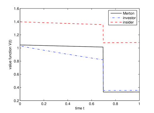
Figure 1: Value function insider vs investor and Merton: $p=0.2$, $\lambda=0.3$ and $\delta=0.5$.

In Figure 2, we fix a smaller short-selling constraint $\delta=0.1$ and we study the impact of the loss given default $\gamma$. We observe that the value functions for both insider and investor are increasing with respect to the loss value $\gamma$. It is interesting to emphasize this phenomenon as a consequence of the short-selling where both insider and the investor will profit the default event and obtain a larger value function. More precisely, in the left-hand figure, we consider a relatively low default risk (with the default intensity $\lambda=0.1$) and we observe that the gain of the insider with respect to the investor remains stable in time and also for different values of $\gamma$. Whereas in the right-hand figure with a higher default risk ($\lambda=0.3$), the impact of $\gamma$ is more important for the investor: before the default the value function of the investor increases more significantly as $\gamma$ increases, and there is no longer a drop at the default time. This can be explained by the fact that the investor has no limit for the short-selling strategy.

Figure 2: Value function insider vs investor: $\delta=0.1$

$$\begin{array}[]{ccc}\includegraphics[width=170.71652pt,angle={270}]{graphe2.eps}&\includegraphics[width=170.71652pt,angle={270}]{graphe1.eps}\\ \mbox{$\lambda=0.1$ }&\mbox{$\lambda=0.3$ }\end{array}$$

Figure 3 shows what may happen in a extreme situation for the default and loss risks. For extreme parameters of default intensity $\lambda=0.5$ and loss value $\gamma=0.5$, we remark that the investor may outperform the insider, see the left-hand figure. In this situation, the investor bet on the occurrence of the default before $T$ and short sell a big amount of the risky asset. The insider value function at time 0 is higher for the investor, and then decreases rapidly until the default time : indeed, as the time goes on and the default has not occurred yet, the risk that the bet turns out to be wrong increases, and thus the value function decreases. At the default time, the investor makes profit of the short selling strategy, the value function being almost doubled. The right-hand figure illustrates the wealth process of the investor on a given scenario in which the default occurs after $T$ despite extreme parameters for the default and loss risks ($\lambda=0.5$ and $\gamma=0.5$). We observe large losses, which are induced by the wrong bet on default and extreme short selling positions.

Figure 3: Extreme scenarios of default : $\lambda=0.5$, $\delta=0.1$

$$\begin{array}[]{ccc}\includegraphics[width=170.71652pt,angle={270}]{graphe4.eps}&\includegraphics[width=170.71652pt,angle={270}]{trajectoire.eps}\\ \mbox{\small{Value function insider vs investor} }&\mbox{\small{Wealth process on one trajectory with $\tau>T$, $\gamma=0.5$} }\end{array}$$

Finally, we study the role of the short-selling limit for different values of $\delta$ in Figure 4. Not surprisingly, the gain of the insider is an increasing function of $\delta$.

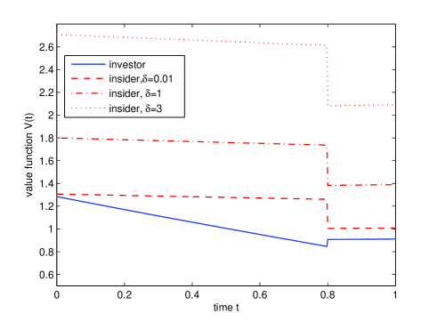
Figure 4: The impact of the short-selling constraint, $\lambda=0.3$ and $\gamma=0.5$.

References

- [1] Amendinger, J., Becherer, D. and Schweizer, M. , 2003. A Monetary Value for Initial Information in Portfolio Optimization, Finance and Stochastics 7, 29-46
- [2] Baudoin, F., 2003. Modelling Anticipations on Financial Markets. Paris-Princeton Lectures on Mathematical Finance, Springer, LNM 1814.
- [3] Benes V. E., 1970. Existence of Optimal Strategies Based on Specified Information for a Class of Stochastic Decision Problems. SIAM Journal of Computation and Optimization, Vol 8 (2), 179-189.
- [4] Bielecki, T.R., Rutkowski, M., 2002. Credit Risk: Modeling, Valuation and Hedging, Springer-Verlag.
- [5] El Karoui, N., Jeanblanc, M. and Jiao, Y., 2010. What Happens After a Default: the Conditional Density Approach. Stochastics Processes and their Applications, 120(7), 1011-1032.
- [6] El Karoui, N., Jeanblanc, M., Jiao, Y. and B. Zargari, 2011. Conditional default probability and density, Musiela Festschrift, to appear.
- [7] Grorud, A., Pontier, M., 1998. Insider Trading in a Continuous Time Market Model, International Journal of Theorical and Applied Finance 1, 331-347.
- [8] Hillairet, C., 2005. Existence of an equilibrium on a financial market with discontinuous prices, asymmetric information and non trivial initial -fields. Mathematical Finance, Vol. 15, No 1, January 2005, 99-117.
- [9] Hillairet, C., Jiao, Y., 2011. Information Asymmetry in Pricing of Credit Derivatives, International Journal of Theoretical and Applied Finance, 14(5), 611-633
- [10] Hillairet, C., Jiao, Y., 2010. Credit Risk with Asymmetric Information on the Default Threshold, Stochastics, to appear.
- [11] Jacod, J., 1979. Calcul stochastique et problèmes de martingales, Lecture Notes 714, Springer-Verlag, New York.
- [12] Jacod, J., 1985. Grossissement Initial, Hypothèse (H’) et Théorème de Girsanov, Lecture Notes 1118, Springer-Verlag, 15-35.
- [13] Jeulin, J., 1980. Semi-martingale et grossissement d’une filtration, Lecture Notes 833, Springer-Verlag.
- [14] Jiao, Y., Pham, H., 2011. Optimal Investment with Counterparty Risk: a Default-Density Model Approach. Finance and Stochastics, 15, 725-753.
- [15] Karatzas, I., Shreve, S.E., 1988. Brownian Motion and Stochastic calculus, Springer-Verlag, New York.