Modulational instability, wave breaking and formation of large scale dipoles in the atmosphere

Abstract

In the present Letter we use the Direct Numerical Simulation (DNS) of the Navier-Stokes equation for a two-phase flow (water and air) to study the dynamics of the modulational instability of free surface waves and its contribution to the interaction between ocean and atmosphere. If the steepness of the initial wave is large enough, we observe a wave breaking and the formation of large scale dipole structures in the air. Because of the multiple steepening and breaking of the waves under unstable wave packets, a train of dipoles is released and propagate in the atmosphere at a height comparable with the wave length. The amount of energy dissipated by the breaker in water and air is considered and, contrary to expectations, we observe that the energy dissipation in air is larger than the one in the water. Possible consequences on the wave modelling and on the exchange of aerosols and gases between air and water are discussed.

The modulational instability, also known as the Benjamin Feir instability, is a well known universal phenomenon that takes place in many different fields of physics such as surface gravity waves, plasma physics, nonlinear optics (see the recent historical review Zakharov and Ostrovsky (2009)). The basic idea consists in that a sufficiently steep sinusoidal wave may become unstable if perturbed by a long enough perturbation. It is a threshold mechanism, therefore, for example, for surface gravity waves in infinite water depth a wave is unstable if $2\sqrt{2}k_{0}A_{0}>\Delta k/k_{0}$, where $k_{0}$ is the wave number of the sinusoidal wave (carrier wave), $\Delta k$ is the wave number of the perturbation and $A_{0}$ is the amplitude of the initial wave.

The modulational instability has been discovered in the sixties and recently it has received again attention because it has been recognized as a possible mechanism of formation of the rogue waves Onorato et al. (2001); Janssen (2003). The standard mathematical tool used to describe such physical phenomena is the Nonlinear Schrördinger equation (NLS), which is a weakly nonlinear, narrow band approximation of some primitive equation of motion. The beauty of such equation is that it is integrable and many analytical solutions can be written explicitly. For example, breather solutions Osborne et al. (2000); Dysthe and Trulsen (1999) have been considered as prototypes of rogue waves; they have been observed in controlled experiments both in surface gravity waves and in nonlinear optics Chabchoub et al. (2011); Clauss et al. (2011); Kibler et al. (2010, 2012).

Concerning the ocean waves, the studies on the modulational instability have been concentrated on the NLS dynamics and only more recently numerical computation of non-viscous, potential, fully nonlinear equations have been considered Dyachenko and Zakharov (2008); Babanin et al. (2007). However, so far none of the aforementioned literature has ever considered the effect of the modulation instability on the fluid above the free surface. As far as we know this is the first attempt in which the dynamics of air on water during the modulation process is investigated. This has been possible by simulating the Navier-Stokes equation for a two phase flow. This approach allows us to investigate conditions which are beyond the formal applicability of the NLS equation: for example, it is well known that if the initial wave steepness is large enough, the NLS equation is not able to describe the dynamics because the breaking of the wave takes place Henderson et al. (1999); Babanin et al. (2011). For steep waves and particularly those close to the breaking onset, vorticity is generated by viscous effects and by the topological change of the interface in case of bubble entrainment processes (this dynamics cannot be described by potential models). Breaking of surface waves, as an oceanic phenomenon Babanin (2011), is important across a very broad range of applications related to wave dynamics, atmospheric boundary layer, air-sea-interactions, upper ocean turbulence mixing, with respective connections to the large-scale processes including ocean circulation, weather and climate Cavaleri et al. (2012). Modulational instability and breaking has become also relevant in engineering applications Clauss et al. (2012) such as naval architecture, structural design of offshore developments, marine transportation, navigation, among many others.

In the present work, the two-fluid flow of air and water is approximated as that of a single incompressible fluid with density and viscosity smoothly varying across the interface. The continuity and momentum equations (Navier-Stokes) are solved in generalized coordinates Iafrati (2009, 2011). The variation of the fluid properties and the surface tension forces is spread across a small neighborhood of the interface. The interface between air and water is captured as the zero level-set of a signed distance from the interface $d({\bm{x}},t)$ which, at $t=0$, is initialized by assuming $d>0$ in water, $d<0$ in air. Physical fluid properties are assumed to be related to $d$ by the equation:

$$f(d)=f_{a}+(f_{w}-f_{a})H_{\delta}(d)$$ (1)

where $H_{\delta}(d)$ is a smooth step function and the parameter $\delta$ is chosen so that the density and viscosity jumps are spread across some grid cells Iafrati and Campana (2005). The distance function is advected in time with the flow as a non-diffusive scalar by using the equation

$$\frac{\partial d}{\partial t}+{\bm{u}}\cdot\nabla d=0,$$ (2)

and the interface is located as the $d=0$ level. Hence, the distance is reinitialized.

In our simulations we consider the standard modulational instability process as the one produced for example in the experimental work in Tulin and Waseda (1999). The initial surface elevation is characterized by a perturbed sinusoidal free surface elevation of the form:

$$\eta(x,t=0)=A_{0}\cos(k_{0}x)+A_{1}(\cos(k^{+}x)+\cos(k^{-}x)),$$ (3)

where $k_{0}$ is the wave number of the carrier wave, $k^{\pm}=k_{0}\pm\Delta k$ with $\Delta k$ the wavenumber of the perturbation. The simulations presented hereafter are characterized by a $\epsilon_{0}=k_{0}A_{0}$ that is varied from $0.1$ to $0.18$, with a step $0.02$. The sideband components are placed at $\Delta k=k_{0}/5$ and their amplitude is $A_{1}=0.1A_{0}$. It is worth noticing that the conditions are essentially similar to those used in Babanin et al. (2007); Song and Banner (2002) and corresponds to the early stages of an Akhmediev breather Akhmediev et al. (1987).

Because of the typical time scale of the modulational instability is of the order of 100 periods, the Navier-Stokes simulation is expensive and for the initial development of the instability a standard potential code is used. The Navier-Stokes simulation is then initialized with solution from the potential flow. For convenience, results are presented in dimensional form. Simulations are carried out for carrier wave of wavelength $\lambda_{0}=0.60$ m, with $g=9.81$ m s^-1. The computational domain which spans horizontally from $x$ = -1.5 m to $x$ = 1.5 m and vertically from $y$= -2 m up to 0.6 m above the still water level. The domain is uniformly discretized in the horizontal direction with $\Delta x$ = 1/1024 m. Vertically, the grid spacing is uniform, and equal to $\Delta x$, from $y$ = -0.15 to 0.15 m whereas it grows geometrically by a factor $\alpha$= 1.03 towards the upper and lower boundaries. This gives a total of 3072 $\times$ 672 grid cells. The total thickness of the transition region is 0.01 m, so that the density jump is spread across about 10 grid cells. Although neglected in the potential flow model, surface tension effects are considered in the Navier-Stokes solution for which the surface tension coefficient is assumed to be that in standard conditions $\sigma=0.073$ N m^-1. In the two-fluid modelling, the densities of air and water are the standard ones, $\varrho_{w}=1000$ kg m^-3 and $\varrho_{a}=1.25$ kg m^-3. The values of the dynamic viscosities in water and air are $\mu_{w}=10^{-3}$ kg m^-1 s^-1 and $\mu_{a}=1.8\,10^{-5}$ kg m^-1 s^-1, respectively.

The process observed in the simulation corresponds to the standard modulational instability (exponential growth of the side bands) up to the point where the wave group reaches its strongly nonlinear regime and eventually wave breaking is observed. We first concentrate our attention to the breaking event: in figure 1 an example for steepness $\epsilon_{0}=k_{0}A_{0}$= 0.18 of the simulation of the wave breaking resulting from the modulational instability is shown; the formation of the first jet is observed which entraps the air. The jet then bounces on the free surface creating a second air bubble. Some droplets of water in air are also visible; a small amount of vorticity is also released beneath the surface.

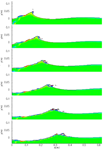
Figure 1: Breaking event for initial steepness $\epsilon_{0}$= 0.18. The color corresponds to the vorticity field: green corresponds to zero vorticity, blue to -20 $sec^{-1}$ and red to 20 $sec^{-1}$.

It is of particular interest to focus the attention on the dynamics of the air flow. In figure 2 we show a sequence of snap-shots of the water and air domain where the formation and detachment of a dipole structure is observed (the simulation is performed for initial steepness of $\epsilon_{0}=0.16$): the rather fast steepening of the wave profile and the wave breaking causes the air flow to separate from the crest giving a rise to large, positive, vorticity structure (positive vorticity is in red). The interaction of this vortex structure with the free surface leads to the formation of a secondary vorticity structure of opposite sign, which eventually detaches from the free surface and forms a dipole which moves under the self-induced velocity (such phenomenon is not observed if the wave breaking process does not take place: we have performed a numerical simulation with $\epsilon_{0}=0.1$ which does not lead to a breaking event and no evident dipole structures have been observed).

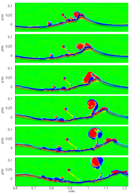
Figure 2: Sequences of formation of a dipole in air as a consequence of the wave breaking. Results refer to an initial steepness $\epsilon_{0}$= 0.16

Because the group velocity is half the phase velocity, each single wave that passes below the group (at its maximum height), breaks. The result is that a series of dipoles are released into the atmosphere as shown in figure 3. Vortices of various sizes and dipoles are clearly observable in the domain. Two things should be noted: i) the height of the highest dipoles is of the order of the wavelength; ii) large amount of vorticity is observed in the air and not in the water.

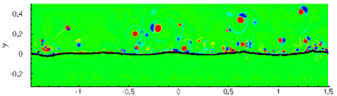
Figure 3: Vorticity field in a portion of the computational domain for initial steepness $\epsilon_{0}=0.18$. The scale of vorticity is as described in the label of figure 1 The supplemental material contains the animation of the simulation (file: animation18.avi).

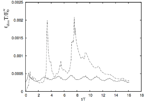
Figure 4: Dissipation nondimensionalized with period $T$ and total energy in the water, $E_{0}^{w}$ a $t=0$ as a function of nondimensional time for water (solid line) and air (dashed line). The initial steepness is 0.12

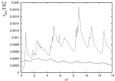
Figure 5: Dissipation nondimensionalized with period $T$ and total energy in the water, $E_{0}^{w}$ a $t=0$ as a function of nondimensional time for water (solid line) and air (dashed line). The initial steepness is 0.18

One major question to be answered, especially in the spirit of modelling the dissipation term in the wave forecasting models Komen et al. (1994); Cavaleri et al. (2007) is the amount of energy dissipated during a wave breaking or a sequence of breaking events. Therefore, a quantitative estimate of the dissipated energy both in air and water can be obtained by integrating the viscous stresses over the air and water domain:

$$\epsilon_{diss}^{w}(t)=\int_{d\geq\delta}2\mu e_{ij}\frac{\partial u_{i}}{\partial x_{j}}\mbox{ d}x\mbox{ d}y,$$ (4)

$$\epsilon_{diss}^{a}(t)=\int_{d<-\delta}2\mu e_{ij}\frac{\partial u_{i}}{\partial x_{j}}\mbox{ d}x\mbox{ d}y,$$ (5)

where $e_{ij}$ is the symmetric part of the strain tensor. In figure 4 and 5 we show the dissipation function normalized by the initial energy of the water and wave period, $T$, as a function of time, nodimensionalized by $T$, for a simulation with steepness $\epsilon_{0}=0.12$ and $\epsilon_{0}=0.18$, respectivelly; the origin of the time axis is set to the time at which the Navier Stokes simulations takes over the simulation with the potential code. The occurrence of spikes in the energy content in the air indicates that an energy fraction is transferred to the air and is successively dissipated by the viscous stresses. The multiple peaks correspond to the the multiple breaking that occurs during the modulational instability process (as mentioned before, the group is slower than the phase velocity and each wave breaks as it passes below it). Similar plots are observed for larger steepness.

In order to show how relevant is the energy dissipation in the air in comparison to the corresponding one in water, we consider the following integrated quantity:

$$E_{diss}(t)=\int_{0}^{t}\epsilon_{diss}(t^{\prime})dt^{\prime}.$$ (6)

The integral is considered for both for water and air. Histories of the integrals in time of the viscous dissipation terms in the two media are shown in figure 6. It is rather interesting to see that, in nondimensional form, the solutions for the four different cases almost overlap, with a total dissipation in the air about three times that in water.

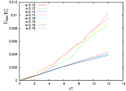
Figure 6: Integrated dissipation for different values of the steepness in water (w) and air (a).

Discussion - Modulated waves of different initial steepnesses have been analyzed using the two phase flow NS equation. For initial steepness larger or equal to 0.12, multiple breaking events have been observed. Spray is the natural consequence of the wave breaking. Droplets of water are thrown in the air; some of these particles are so small (aerosols) that they can remain in the air for a very long time, forming condensation nuclei for clouds and affecting incoming solar radiation and therefore relevant for climate modelling. Vortices, observed in our simulations, can in principle transport aerosols (not resolved in our simulations) up to the height of the wave lengths (this can be even underestimated because of the presence of the solid boundary at the top of the computational domain). Quantitative analyses of the energy contents and of the viscous dissipation term have been provided. Even bearing in mind the limits of the numerical scheme, the results indicate that, due to the highly rotational flow in air, the dissipation of the energy is mostly concentrated in the air side. We stress that it is a common practice to estimate the energy loss due to a wave breaking by looking at the amount of energy dissipate in the water, see for example Terray et al. (1996). Such measurement are the bases for the construction of the dissipation function in the operational wave forecasting modelling Cavaleri et al. (2007). If the modulational instability is responsible of the wave breaking in the ocean, then such results would clearly lead to an underestimation of the the total energy dissipated. The present work represents the first attempt to study the modulational instability starting from the Navier-Stokes equation and its effects on water and air. Clearly, it has a number of limitation due to the heaviness of the computation. Probably the most important one is that we have assumed that waves are long crested and the fluid domain is 2-dimensional. In reality, we expect that 3D effects can take place and dipoles and vortices can become unstable. We also underline that our simulations correspond to the propagation of waves without the presence of external wind: what would be the consequences of a turbulent wind on the generation of vorticity during breaking event is under investigation.

Acknowledgments M.O. has been funded by EU, project EXTREME SEAS (SCP8-GA-2009-234175) and by ONR grant N000141010991. Dr. Proment and Dr. Giulinico are acknowledged for discussion. The work by A.I. has been done within the RITMARE research project.

References

- Zakharov and Ostrovsky (2009) V. Zakharov and L. Ostrovsky, Physica D: Nonlinear Phenomena 238, 540 (2009).
- Onorato et al. (2001) M. Onorato, A. Osborne, M. Serio, and S. Bertone, Phys. Rev. Lett. 86, 5831 (2001).
- Janssen (2003) P. A. E. M. Janssen, J. Phys. Ocean. 33, 863 (2003).
- Osborne et al. (2000) A. Osborne, M. Onorato, and M. Serio, Phys. Lett. A 275, 386 (2000).
- Dysthe and Trulsen (1999) K. B. Dysthe and K. Trulsen, Physica Scripta T82, 48 (1999).
- Chabchoub et al. (2011) A. Chabchoub, N. Hoffmann, and N. Akhmediev, Physical Review Letters 106, 204502 (2011).
- Clauss et al. (2011) G. Clauss, M. Klein, and M. Onorato (Proceedings of the ASME 2011 30th International Conference on Ocean, Offshore and Arctic Engineering OMAE2011, June 19 24, 2011, Rotterdam, The Netherlands., 2011).
- Kibler et al. (2010) B. Kibler, J. Fatome, C. Finot, G. Millot, F. Dias, G. Genty, N. Akhmediev, and J. Dudley, Nature Physics 6, 790 (2010), ISSN 1745-2473.
- Kibler et al. (2012) B. Kibler, J. Fatome, C. Finot, G. Millot, G. Genty, B. Wetzel, N. Akhmediev, F. Dias, and J. Dudley, Scientific reports 2 (2012).
- Dyachenko and Zakharov (2008) A. Dyachenko and V. Zakharov, JETP letters 88, 307 (2008).
- Babanin et al. (2007) A. Babanin, D. Chalikov, I. Young, and I. Savelyev, Geophys. Res. Lett 34, L07605 (2007).
- Henderson et al. (1999) K. Henderson, D. Peregrine, and J. Dold, Wave Motion 29, 341 (1999).
- Babanin et al. (2011) A. Babanin, T. Waseda, T. Kinoshita, and A. Toffoli, Journal of Physical Oceanography 41, 145 (2011).
- Babanin (2011) A. Babanin, Breaking and dissipation of ocean surface waves (Cambridge Univ Pr, 2011).
- Cavaleri et al. (2012) L. Cavaleri, B. Fox-Kemper, and M. Hemer, Bulletin of the American Meteorological Society, Accepted for pubblication (2012).
- Clauss et al. (2012) G. F. Clauss, M. Klein, M. Dudek, and M. Onorato (Proceedings of the ASME 2012 31th International Conference on Ocean, Offshore and Arctic Engineering OMAE2012, July 1 6, 2012, Rio de Janeiro, Brazil, 2012).
- Iafrati (2009) A. Iafrati, Journal of Fluid Mechanics 622, 371 (2009).
- Iafrati (2011) A. Iafrati, Journal of Geophysical Research 116, C07024 (2011).
- Iafrati and Campana (2005) A. Iafrati and E. Campana, Journal of Fluid Mechanics 529, 311 (2005).
- Tulin and Waseda (1999) M. P. Tulin and T. Waseda, J. Fluid Mech. 378, 197 (1999).
- Song and Banner (2002) J. Song and M. Banner, J. Phys. Ocean. 32, 2541 (2002).
- Akhmediev et al. (1987) N. Akhmediev, V. Eleonskii, and N. Kulagin, Theoretical and Mathematical Physics 72, 809 (1987), ISSN 0040-5779.
- Komen et al. (1994) G. Komen, L. Cavaleri, M. Donelan, K. Hasselmann, H. Hasselmann, and P. Janssen, Dynamics and modeling of ocean waves (Cambridge University Press, Cambridge, 1994).
- Cavaleri et al. (2007) L. Cavaleri, J. Alves, F. Ardhuin, A. Babanin, M. Banner, K. Belibassakis, M. Benoit, M. Donelan, J. Groeneweg, T. Herbers, et al., Progress in Oceanography 75, 603 (2007).
- Terray et al. (1996) E. Terray, M. Donelan, Y. Agrawal, W. Drennan, K. Kahma, A. Williams, P. Hwang, and S. Kitaigorodskii, Journal of Physical Oceanography 26, 792 (1996).