Local Quantile Regression

Abstract

Quantile regression is a technique to estimate conditional quantile curves. It provides a comprehensive picture of a response contingent on explanatory variables. In a flexible modeling framework, a specific form of the conditional quantile curve is not a priori fixed. This motivates a local parametric rather than a global fixed model fitting approach. A nonparametric smoothing estimator of the conditional quantile curve requires to balance between local curvature and stochastic variability. In this paper, we suggest a local model selection technique that provides an adaptive estimator of the conditional quantile regression curve at each design point. Theoretical results claim that the proposed adaptive procedure performs as good as an oracle which would minimize the local estimation risk for the problem at hand. We illustrate the performance of the procedure by an extensive simulation study and consider a couple of applications: to tail dependence analysis for the Hong Kong stock market and to analysis of the distributions of the risk factors of temperature dynamics.

Keywords: local MLE, excess bound, propagation condition, adaptive bandwidth selection.

JEL classification: C00, C14, J01, J31

1 Introduction

Quantile regression is gradually developing into a comprehensive approach for the statistical analysis of linear and nonlinear response models. Since the rigorous treatment of linear quantile regression by Keo:bas:1987, richer models have been introduced into the literature, among them are nonparametric, semiparametric and additive approaches. Quantile regression or conditional quantile estimation is a crucial element of analysis in many quantitative problems. In financial risk management, the proper definition of quantile based Value at Risk impacts asset pricing, portfolio hedging and investment evaluation, eng:man:2004, cai:wan:08 and fit:wil:08. In labor market analysis of wage distributions, education effects and earning inequalities are analyzed via quantile regression. Other applications of conditional quantile studies include, for example, conditional data analysis of children growth and ecology, where it accounts for the unequal variations of response variables, see ja:ha:10.

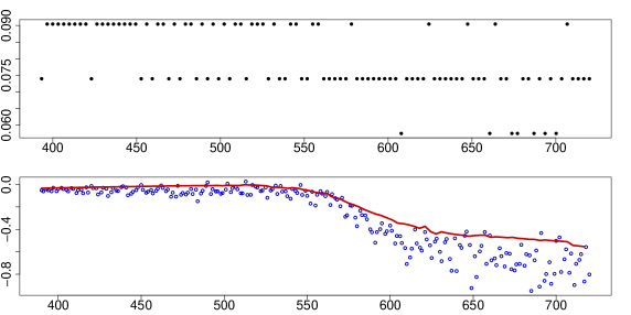
Figure 1: The bandwidth sequence (upper panel), plot of data and the estimated $\,90\%\,$ quantile curve (lower panel)

In applications, the predominantly used linear form of the calibrated models is mainly determined by practical and numerical reasonings. There are many efficient algorithms (like sparse linear algebra and interior point methods) available, St:Ro:89, St:Ro:97, Jo:Ro:99, and Ro:2005, etc. However, the assumption of a linear parametric structure can be too restrictive in many applications. This observation spawned a stream of literature on nonparametric modeling of quantile regression, yu:jo:98, Fan:Hu:94, etc. One line of thought concentrated on different smoothing techniques, e.g. splines, kernel smoothing, etc.; see fan:1996. Another line of literature considers structural semiparametric models to cope with the curse of dimensionality, like, partial linear models, ha:so:ya:10, etc., additive models, KLX08, jo:lee:05, etc; single index models, wu:yu:10, Ro:10, etc. Yet another strand of literature has been involved in ultra-high dimensional situations where a careful variable selection technique needs to be implemented, al:vi:10 and Ro:10. In most of the aforementioned papers on non and semiparametric quantile regression, a smoothing parameter selection is implicit, and it is mostly a consequence of theoretical assumptions like e.g. degree of smoothness, but falls short in practical hints for real data applications. An important exception is the method for local nonparametric kernel smoothing by yu:jo:98 and cai:xu:08. They both propose a data driven bandwidth choice.

This paper offers a novel data-driven quantile regression procedure. Its numerical performance is illustrated by competitive simulation examples and applications to real data. The proposed adaptive local quantile regression algorithm is easy to implement and works for a wide class of applications. The idea of this algorithm is to select the bandwidth locally by a sequence of likelihood ratio tests. We also provide a rigorous theoretical study for the proposed method. The optimality results are stated as exact and sharp oracle risk bounds. In particular, we show that the performance of the adaptive procedure is essentially the same as the best possible one. The results apply for finite sample and under mild regularity conditions.

The main message is that the proposed algorithm is spatially adaptive, stable in homogeneous situation and sensitive to structural changes of the quantile curve. This conclusion is justified by theoretical results and confirmed by the numerical study. As an example, consider Figure 1 which presents our results for analyzing the Lidar data set, Ru:2003. The presented quantile curve switches smoothness in the middle, and it is naturally reflected by the bandwidth sequence (upper panel) selected. In the presence of changing to sharper slope of the curve, the bandwidths get smaller to attain better approximations. This example shows that the algorithm proposed in this paper can adaptively choose the bandwidth at each design point.

This article is organized as follows. Section 2 introduces the local model selection (LMS) procedure and explains how to important tuning parameters (critical values) can be computed. Section LABEL:SsimulLQR presents a number of Monte Carlo simulations to illustrate the proposed methodology. In Section LABEL:SapplLQR the method is applied to check the tail dependency among portfolio stocks, and estimate quantile curves for temperature risk factors. Section LABEL:StheoryLQR presents our main theoretical result which states a kind of oracle risk bound for the proposed procedure: it performs nearly as good as the best one among the considered family of local quantile estimators. The necessary conditions and main steps of the proof like “propagation”, “stability” and “oracle” property are delegated to the Appendix. There we also collect some of general results like majorization bounds and non-asymptotic Wilks Theorem for the likelihood ratio test statistics.

2 Adaptive estimation procedure

This section introduces the considered problem and offers an adaptive estimation procedure.

2.1 Quantile regression model

Given the quantile level $\,\tau\in(0,1)\,$, the quantile regression model describes the following relation between the response $\,Y\,$ and the regressor $\,X\,$: [c] P(Y ¿ f(x)   —  X=x) = τ, where $\,f(x)\,$ is the unknown quantile regression function. This function is the target of the analysis and it has to be estimated from independent observations $\,\{X_{i},Y_{i}\}_{i=1}^{n}\,$. For the case of a deterministic design, this quantile relation can be represented as [c] Y_i = f(X_i) + ε_i   , where the errors $\,\varepsilon_{i}\,$ follow $\,\boldsymbol{P}(\varepsilon_{i}>0)=\tau\,$.

For simplicity of presentation, we consider a univariate regressor $\,X\in I\!\!R^{1}\,$ and a deterministic design in this paper, an extension to the $\,d\,$-dimensional case $\,X\in I\!\!R^{d}\,$ with $\,d>1\,$ is straightforward.

2.2 A qMLE View on Quantile Estimation

The quantile function $\,f(\cdot)\,$ in (eq:model) is usually recovered by minimizing the sum [c] ∑_i=1^n ρ_τ{Y_i - f(X_i) } , over the class of all considered quantile functions $\,f(\cdot)\,$, where [c] ρ_τ(u) =defu {τ1I(u≥0) - (1-τ)1I(u¡0)} = u { τ- 1I(u¡0) }. Such an approach is reasonable because the true quantile function $\,f(x)\,$ minimizes the expected value of the sum in (2.2). An important special case is given by $\,\tau=1/2\,$. Then an estimator of $\,f(\cdot)\,$ is built as minimizer of the least absolute deviations (LAD) contrast $\,\sum|Y_{i}-f(X_{i})|\,$.

The minimum contrast approach based on minimization of (2.2) can also be put in a quasi maximum likelihood framework. Assume that the residuals $\,\varepsilon_{i}\,$ from (2.1) are i.i.d. and $\,\ell(x)\,$ is their negative log-density on $\,I\!\!R^{1}\,$. Then the joint log-density is given by the sum [c] - ∑ℓ{ Y_i - f(X_i) } and its maximization is equivalent to minimization of the contrast (2.2) with a pdf from the asymmetric Laplace distribution $\,ALD_{\tau}\,$: [c] ℓ(u) = ℓ_τ(u) = log{ τ(1-τ) } - ρ_τ(u),  -∞¡ u ¡ ∞. The parametric approach (PA) assumes that the quantile regression function $\,f(\cdot)\,$ belongs to a family of functions $\,\bigl{\{}f_{\boldsymbol{\theta}}(x),\,\boldsymbol{\theta}\in\varTheta\bigr{\}}\,$, where $\,\varTheta\,$ is a subset of the $\,(p+1)\,$-dimensional Euclidean space. Equivalently, [c] f(x) = f_θ^*(x), where $\,\boldsymbol{\theta}^{*}\,$ is the true parameter which is usually the target of estimation.

Examples are a constant model: [c] f_θ^*(x) ≡θ_0, with $\,\theta^{*}=\theta_{0}\,$ or a linear model: [c] f_θ^*(x) = θ_0 + θ_1x, with $\,\boldsymbol{\theta}^{*}=(\theta_{0},\theta_{1})^{\top}\,$.

Let $\,\boldsymbol{P}_{\boldsymbol{\theta}}\,$ be the parametric measure on the observation space which corresponds to the regression model (2.1) with $\,f(\cdot)\equiv f_{\boldsymbol{\theta}}(\cdot)\,$ and with the i.i.d. errors $\,\varepsilon_{i}\,$ following the asymmetric Laplace distribution (2.2). Then the log-likelihood $\,L(\boldsymbol{\theta})=L(\boldsymbol{Y},\boldsymbol{\theta})\,$ for $\,\boldsymbol{P}_{\boldsymbol{\theta}}\,$ can be written as L(θ) & =def log{ τ(1-τ) } ∑_i=1^n 1 - ∑_i=1^n ρ_τ {Y_i - f_θ(X_i)} and the qMLE $\,\widetilde{\boldsymbol{\theta}}\,$ maximizes $\,L(\boldsymbol{\theta})\,$, or, equivalently minimizes the contrast $\,\sum_{i=1}^{n}\rho_{\tau}\{Y_{i}-f_{\boldsymbol{\theta}}(X_{i})\}\,$ over all $\,\boldsymbol{\theta}\in\varTheta\,$.

The described parametric construction is based on two assumptions: one is about the error distribution (2.2) and the other one is about the shape of the regression function $\,f\,$. However, it is only used for motivating our approach. Our theoretical study will be done under the true data distribution which follows (2.1) under mild regularity conditions. The next section explains how a smooth regression function $\,f\,$ can be modeled by a flexible local parametric assumption.

2.3 Local polynomial qMLE

This section explains how the restrictive global PA $\,f(\cdot)\equiv f_{\boldsymbol{\theta}^{*}}(\cdot)\,$ can be relaxed by using a local parametric approach. Let a point $\,x\,$ be fixed. The local PA at a point $\,x\in I\!\!R\,$ only requires that the quantile regression function $\,f(\cdot)\,$ can be approximated by a parametric function $\,f_{\boldsymbol{\theta}}(\cdot)\,$ from the given family in a vicinity of $\,x\,$. Below we fix a family of polynomial functions of degree $\,p\,$ motivated by Taylor approximation: [c] f(u) ≈f_θ =defθ_0 + θ_1(u-x) + …+ θ_p(u-x)^p/p! for $\,\boldsymbol{\theta}=(\theta_{0},\ldots,\theta_{p})^{\top}\,$. The corresponding parametric model can be written as [c] Y_i = Ψ_i^⊤ θ+ ε_i   , where $\,\varPsi_{i}=\{1,(X_{i}-x),(X_{i}-x)^{2}/2!,\ldots,(X_{i}-x)^{p}/p!\}^{\top}\in I\!\!R^{p+1}\,$.

A local likelihood approach at $\,x\,$ is specified by a localizing scheme $\,W\,$ given by a collection of weights $\,w_{i}\,$ for $\,i=1,\ldots,n\,$. The weights $\,w_{i}\,$ vanish for points $\,X_{i}\,$ lying outside a vicinity of the point $\,x\,$. A standard proposal for choosing the weights $\,W\,$ is $\,w_{i}=K_{\operatorname{loc}}\{(X_{i}-x)/h\}\,$, where $\,K_{\operatorname{loc}}(\cdot)\,$ is a kernel function with a compact support, while $\,h\,$ is a bandwidth controlling the degree of localization.

Define now the local log-likelihood at $\,x\,$ by [c] L(W,θ) =deflogτ(1-τ) ∑_i=1^n w_i - ∑_i=1^n ρ_τ(Y_i - Ψ_i^⊤ θ) w_i   . This expression is similar to the global log-likelihood in (2.2), but each summand in $\,L(W,\boldsymbol{\theta})\,$ is multiplied with the weight $\,w_{i}\,$, so only the points from the local vicinity of $\,x\,$ contribute to $\,L(W,\boldsymbol{\theta})\,$. Note that this local log-likelihood depends on the central point $\,x\,$ via the structure of the basis vectors $\,\varPsi_{i}\,$ and via the weights $\,w_{i}\,$. The corresponding local qMLE at $\,x\,$ is defined via maximization of $\,L(W,\boldsymbol{\theta})\,$: ~θ(x) &= {~θ_0(x),~θ_1(x),…,~θ_p(x)}^⊤
=def argmax_θ∈Θ L(W,θ)
= argmin_θ∈Θ ∑_i=1 ρ_τ(Y_i - Ψ_i^⊤ θ) w_i   . The first component $\,\widetilde{\theta}_{0}(x)\,$ provides an estimator of $\,f(x)\,$, while $\,\widetilde{\theta}_{m}(x)\,$ is an estimator of the derivative $\,f^{(m)}(x)\,$, $\,m=1,\ldots,p\,$.

2.4 Selection of a Pointwise Bandwidth

The choice of bandwidth $\,h\,$ is an important issue in implementing (eq:non). One can reduce the variance of the estimation by increasing the bandwidth, but at a price of possibly inducing more modeling bias measured by the accuracy of approximation in (2.3); see Figure 2.

A desirable choice of a bandwidth at a fixed point would strike a balance between the variance and the bias depending on the local shape of $\,f(\cdot)\,$ in the vicinity of $\,x\,$. Many approaches have been proposed along this line; see e.g. yu:jo:98 and references therein. However, their justification and implementation is based on asymptotic arguments and require large samples. Here we propose a pointwise bandwidth selection technique based on a finite sample theory.

Our basic setup of the algorithm is described as follows. First one fixes a finite ordered set of possible bandwidths $\,h_{1}<h_{2}<\ldots<h_{K}\,$, where $\,h_{1}\,$ is very small, while $\,h_{K}\,$ should be a global bandwidth of the order of the design range. The bandwidth sequence can be taken geometrically increasing of the form $\,h_{k}=ab^{k}\,$ with fixed $\,a>0\,$, $\,b>1\,$, and $\,n^{-1}<ab^{k}<1\,$ for $\,k=1,\ldots,K\,$ ($\,\text{{A}}.2.\,$). The total number $\,K\,$ of the candidate bandwidths is then at most logarithmic in the sample size $\,n\,$. For each $\,k\leq K\,$, an ordered weighting schemes $\,W^{(k)}=(w^{(k)}_{1},w^{(k)}_{2},\ldots,w^{(k)}_{n})^{\top}\,$ is defined via $\,w_{i}^{(k)}\stackrel{{\scriptstyle\operatorname{def}}}{{=}}K_{\operatorname{loc}}\{(x-X_{i})/h_{k}\}\,$ leading to a local quantile estimator $\,\widetilde{\boldsymbol{\theta}}_{k}(x)\,$ with [c] ~θ_k(x) = argmax_θ∈Θ L(W^(k),θ) = argmin_θ∈Θ ∑_i=1 ρ_τ(Y_i - Ψ_i^⊤ θ) w_i^(k)   . The proposed selection procedure is similar in spirit to le:ma:96. If the underlying quantile regression function is smooth, one can expect a good quality of approximation (2.3) for a large bandwidth among $\,\{h_{k}\}_{k=1}^{K}\,$. Moreover, if the approximation is good for one bandwidth, it will be also suitable for all smaller bandwidths. So, if we observe a significant difference between the estimator $\,\widetilde{\boldsymbol{\theta}}_{k}(x)\,$ corresponding to the bandwidth $\,h_{k}\,$ and an estimator $\,\widetilde{\boldsymbol{\theta}}_{\ell}(x)\,$ corresponding to a smaller bandwidth $\,h_{\ell}\,$, this is an indication that the approximation (2.3) for the window size $\,h_{k}\,$ becomes too rough. This justifies the following algorithm. Start with the smallest bandwidth $\,h_{1}\,$. For any $\,k>1\,$, compute the local qMLE $\,\widetilde{\boldsymbol{\theta}}_{k}(x)\,$ and check whether it is consistent with all the previous estimators $\,\widetilde{\boldsymbol{\theta}}_{\ell}(x)\,$ for $\,\ell<k\,$. If the consistency check is negative, the procedure terminates and selects the latest accepted estimator.

The most important ingredient of the method is the consistency check. The Lepski method suggests to use the difference $\,\widetilde{\boldsymbol{\theta}}_{k}(x)-\widetilde{\boldsymbol{\theta}}_{\ell}(x)\,$ as a test statistic; see e.g. le:ma:96. We follow the suggestion from Polzehl:2006 and apply a localized likelihood ratio type test. More precisely, the local MLE $\,\widetilde{\boldsymbol{\theta}}_{\ell}(x)\,$ maximizes the log-likelihood $\,L\bigl{(}W^{(\ell)},\boldsymbol{\theta}\bigr{)}\,$, and the maximal value of (2.3) given by $\,\sup_{\boldsymbol{\theta}}L\bigl{(}W^{(\ell)},\boldsymbol{\theta}\bigr{)}=L\bigl{(}W^{(\ell)},\widetilde{\boldsymbol{\theta}}_{\ell}(x)\bigr{)}\,$ is compared with the particular log-likelihood value $\,L\bigl{(}W^{(\ell)},\widetilde{\boldsymbol{\theta}}_{k}(x)\bigr{)}\,$, where the estimator $\,\widetilde{\boldsymbol{\theta}}_{k}(x)\,$ is obtained by maximizing the other local log-likelihood function $\,L(W^{(k)},\boldsymbol{\theta})\,$. The difference $\,L\bigl{(}W^{(\ell)},\widetilde{\boldsymbol{\theta}}_{\ell}(x)\bigr{)}-L\bigl{(}W^{(\ell)},\widetilde{\boldsymbol{\theta}}_{k}(x)\bigl{)}\,$ is always non-negative. The check rejects $\,\widetilde{\boldsymbol{\theta}}_{k}(x)\,$ if this difference is too large for some $\,\ell<k\,$. Equivalently one can say that the test checks whether $\,\widetilde{\boldsymbol{\theta}}_{k}(x)\,$ belongs to the confidence sets $\,\mathscr{E}_{\ell}(\mathfrak{z})\,$ of $\,\widetilde{\boldsymbol{\theta}}_{\ell}(x)\,$: [c] E_ℓ(z) =def{ θ∈Θ: L( W^(ℓ),~θ_ℓ(x) ) - L( W^(ℓ),θ) ≤z} . A great advantage of the likelihood ratio test is that the critical value $\,\mathfrak{z}\,$ can be selected universally. This is justified by the Wilks phenomenon: the likelihood ratio test statistics is nearly $\,\chi^{2}\,$ and its asymptotic distribution depends only on the dimension of the parameter space. Unfortunately, these arguments do not apply to finite samples under possible model misspecification and we therefore offer an alternative way of fixing the critical values $\,\mathfrak{z}\,$ which is based on the so called propagation condition. We also allow that the width of the confidence set $\,\mathscr{E}_{\ell}(\mathfrak{z})\,$ depends on the index $\,\ell\,$, that is, $\,\mathfrak{z}=\mathfrak{z}_{\ell}\,$. Our adaptation algorithm can be summarized as follows: at each step $\,k\,$, an estimator $\,\widehat{\boldsymbol{\theta}}_{k}(x)\,$ is constructed based on the first $\,k\,$ estimators $\,\widetilde{\boldsymbol{\theta}}_{1}(x),\ldots,\widetilde{\boldsymbol{\theta}}_{k}(x)\,$ by the following rule,

• Start with $\,\widehat{\boldsymbol{\theta}}_{1}(x)=\widetilde{\boldsymbol{\theta}}_{1}(x)\,$.

• For $\,k\geq 2\,$, $\,\widetilde{\boldsymbol{\theta}}_{k}(x)\,$ is accepted and $\,\widehat{\boldsymbol{\theta}}_{k}(x)\stackrel{{\scriptstyle\operatorname{def}}}{{=}}\widetilde{\boldsymbol{\theta}}_{k}(x)\,$, if $\,\widetilde{\boldsymbol{\theta}}_{k-1}(x)\,$ was accepted and [c] L( W^(ℓ),~θ_ℓ(x) ) - L( W^(ℓ),~θ_k(x) ) ≤z_ℓ,   ℓ= 1,…,k-1 .

• Otherwise $\,\widehat{\boldsymbol{\theta}}_{k}(x)=\widehat{\boldsymbol{\theta}}_{k-1}(x)\,$.

The adaptive estimator $\,\widehat{\boldsymbol{\theta}}(x)\,$ is the latest accepted estimator after all $\,K\,$ steps: [c] ^θ(x) =def^θ_K(x) A visualization of the procedure is presented in Figure 2. The critical values $\,\mathfrak{z}_{\ell}\,$’s are selected by an algorithm based on the propagation condition explained in the next section.

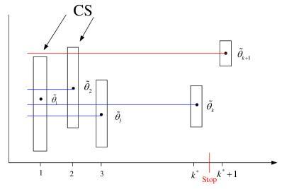
Figure 2: Demonstration of the local adaptive algorithm.

2.5 Parameter Tuning by Propagation Condition

The practical implementation requires to fix the critical values of $\,\mathfrak{z}_{1},\ldots,\mathfrak{z}_{K-1}\,$. We apply the propagation approach which is an extension of the proposal from Spokoiny:2009; SV2007. The idea is to tune the parameter of the procedure for one artificial parametric situation. Later we show that such defined critical values work well in the general setup and provide a nearly efficient estimation quality. The presented bandwidth selector can be viewed as a multiple testing procedure. This suggests fixing the critical values as in the general testing theory by ensuring a prescribed performance under the null hypothesis. In our case, the null hypothesis corresponds to the pure parametric situation with $\,f(\cdot)\equiv f_{\boldsymbol{\theta}^{*}}(\cdot)\,$ in the equation (2.1). Moreover, we fix some particular distribution of the errors $\,\varepsilon_{i}\,$, our specific choice is $\,ALD_{\tau}\,$ with parameter $\,\tau\,$. Below in this section we denote by $\,\boldsymbol{P}_{\boldsymbol{\theta}^{*}}\,$ the data distribution under these assumptions.

For this artificial data generating process, all the estimators $\,\widetilde{\boldsymbol{\theta}}_{k}(x)\,$ should be consistent to each other and the procedure should not terminate at any intermediate step $\,k<K\,$. This effect is called as propagation: in the parametric situation, the degree of locality will be successfully increased until it reaches the largest scale. The critical values are selected to ensure the desired propagation condition which effectively means a “no false alarm” property: the selected adaptive estimator coincides in the most cases with the estimator $\,\widetilde{\boldsymbol{\theta}}_{K}(x)\,$ corresponding to the largest bandwidth. The event $\,\bigl{\{}\widetilde{\boldsymbol{\theta}}_{k}(x)\neq\widehat{\boldsymbol{\theta}}_{k}(x)\bigr{\}}\,$ for $\,k\leq K\,$ is associated with a false alarm and the corresponding loss can be measured by the difference [c] L( W^(k),~θ_k(x),^θ_k(x) ) =defL( W^(k),~θ_k(x) ) - L( W^(k),^θ_k(x) ) . The propagation condition postulates that the risk induced by such false alarms is smaller than the upper bound for the risk of the estimator $\,\widetilde{\boldsymbol{\theta}}_{k}(x)\,$ in the pure parametric situation: [c] E_θ^* L^r( W^(k),~θ_k(x),^θ_k(x) ) ≤αR_r   k=2,…,K, where the constant $\,\mathscr{R}_{r}\,$ is such that for all $\,k\leq K\,$, it holds [c] E