Outflowing activity in the UCHII region G045.47+0.05

Abstract

Aims. This work aims at investigating the molecular gas in the surroundings of the ultra-compact HII region G045.47+0.05 looking for evidence of molecular outflows.

Methods. We carried out observations towards a region of 2^′$\times$2^′ centered at RA=19^h14^m25.6^s, dec.=+11^∘09^′27.6^′′(J2000) using the Atacama Submillimeter Telescope Experiment (ASTE; Chile) in the ¹²CO J=3–2, ¹³CO J=3–2, HCO⁺ J=4–3 and CS J=7–6 lines with an angular resolution of 22^′′. We complement these observations with public infrared data.

Results. We characterize the physical parameters of the molecular clump where G045.47+0.0 is embedded. The detection of the CS J=7–6 line emission in the region reveals that the ultra-compact HII region G045.47+0.0 has not completely disrupted the dense gas where it was born. The HCO⁺ abundance observed towards G045.47+0.0 suggests the presence of molecular outflow activity in the region. From the analysis of the ¹²CO J=3–2 transition we report the presence of bipolar molecular outflows with a total mass of about 300 M_⊙. We derive a dynamical time (flow’s age) of about $10^{5}$ yr for the outflow gas, in agreement with the presence of an ultra-compact HII region. We identify the source 2MASS 19142564+1109283 as the massive protostar candidate to drive the molecular outflows. Based on the analysis of its spectral energy distribution we infer that it is an early B-type star of about 15 M_⊙. The results of this work support the scenario where the formation of massive stars, at least up to early B-type stars, is similar to that of low mass stars.

1 Introduction

The formation of high-mass stars remains one of the most significant unsolved problems in astrophysics. Despite the importance that massive stars have in the structure and dynamic of the Galaxy, the physical processes involved in their formation are less understood than those of their low-mass counterpart. Observationally, the main problems arise from the fact that they are heavily obscured by dust, are rare, and evolve very fast, making their detection very difficult. The study of massive star formation also poses major theoretical challenges because they begin burning their nuclear fuel and radiating prodigious amounts of energy while still accreting. If the formation of massive stars is similar to that of low mass stars (i.e. via accretion from the surrounding envelope), a mass accretion rate $\dot{M}$ of at least several orders of magnitude above the values appropriate for the low mass star formation is required (Tan & McKee, 2002). At present, two theoretical scenarios are proposed to explain the formation of these stars: a monolithic collapse of turbulent gas on the scale of massive dense cores (Tan & McKee, 2002), which is a scaled-up version of the low-mass star formation picture, and a competitive one where accretion occurs inside the gravitational potential of a cluster-forming massive dense core (Bonnell & Bate, 2006). This last model predicts that stars located near the center of the full gravitational potential accrete at much higher rates than do isolated stars.

The detection of molecular outflows associated with both, high and low-mass young stellar objects, supports a scaled-up formation picture (Beuther, 2002a). In this context, the study of massive molecular outflows and the associated driving source might contribute to discern which is the scenario that prevails in a given star forming region.

It is well known that the generation of molecular outflows during the formation of a high-mass star is a phenomenon that can take place even when the UCHII region stage has been reached (Hunter et al. 1997; Qin et al. 2008). In this work we report the study of the UCHII region G045.47+0.05 (hereafter G45.47), through the analysis of its associated molecular gas and searching for evidence of molecular outflows and its associated driving source. G45.47 was first detected by Wood & Churchwell (1989) in radio continuum at 6 cm. This object is adjacent to the extensively studied UCHII region G45.45+0.06 (hereafter G45.45), which is part of a complex of five radio compact HII regions (Matthews et al. 1977; Giveon et al. 2005a; Giveon et al. 2005b). Such complex and G45.47 are embedded in the molecular cloud GRSMC G045.49+00.04 (at V${}_{LSR}\sim$ 58 km s^-1; Rathborne et al. 2009) and are located on the northern border of the more extended HII region named G45L in Paron et al. (2009). Based on HI absorption profiles, Kuchar & Bania (1994) derived a kinematics distance of 8.3 kpc for the UCHII region G45.45. As G45.47 is part of the same complex, we adopt for this object the same distance.

Caswell et al. (1995) detected a class II CH₃OH maser emission at 6.6 GHz at V${}_{LSR}\sim 56$ km s^-1  towards G45.47. Given that the 6.6 GHz methanol maser is radiatively pumped by IR emission from the warm dust associated exclusively with massive young stellar object (MYSOs) their detection is useful to study the kinematic of the gas and, in particular, to establish the systemic velocity (Cyganowski et al., 2009).

Based on high resolution molecular line observations towards G45.47, Wilner et al. (1996) identified five HCO⁺ (1–0) clumps and suggested that G45.47 is in the early stages of the formation of an OB cluster. From an ammonia absorption study, Hofner et al. (1999) suggested the presence of a remnant molecular core infalling onto the UCHII region. Later, Cyganowski et al. (2008) identified an “Extended Green Object” (EGO) at the position of G45.47, the EGO G45.47+0.05. Their identification as EGOs comes from the common coding of the 4.5 $\mu$m band as green in the three-color composite Infrared Array Camera (IRAC; Fazio et al. 2004) images from the Spitzer Telescope. Extended 4.5 $\mu$m emission is thought to evidence the presence of shocked molecular gas in protostellar outflows. The association of EGOs with IRDCs and 6.7 GHz CH₃OH maser suggests that EGOs trace the formation of massive protostars. According to Cyganowski et al. (2008), an EGOs is a MYSO with ongoing outflow activity and actively accreting.

In summary, G45.47 is a rich and complex region to study the formation of a new generation of massive stars. In this paper we present a new study of the dense ambient medium where the UCHII region is evolving. We investigate the molecular gas through several molecular lines observed with the Atacama Submillimeter Telescope Experiment (ASTE; Chile) and characterize the central source based on infrared public data.

2 Data

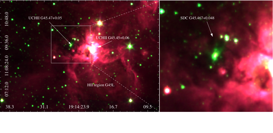
Figure 1: Spitzer-IRAC three color images (3.6 $\mu$m = blue, 4.5 $\mu$m = green and 8 $\mu$m = red). The white box in the left panel indicates the region mapped with ASTE. A close up view of this region is shown in the right panel. Red, green and blue scales go from 30 to 500, from 2 to 110, and from 1 to 80 MJy/sr, respectively.

The molecular line observations were carried out on June 12 and 13, 2011 with the 10 m Atacama Submillimeter Telescope Experiment (ASTE; Ezawa et al., 2004). We used the CATS345 GHz band receiver, which is a two-single band SIS receiver remotely tunable in the LO frequency range of 324-372 GHz. We simultaneously observed ¹²CO J=3$-$2 at 345.796 GHz and HCO⁺ J=4$-$3 at 356.734 GHz, mapping a region of 2^′$\times$2^′  centered at RA = 19^h14^m25.6^s, dec.=+11^∘09^′27.6^′′(J2000). We also observed ¹³CO J=3$-$2 at 330.588 GHz and CS J=7$-$6 at 342.883 GHz towards the same region. The mapping grid spacing was 20^′′ in both cases and the integration time was 20 sec (¹²CO and HCO⁺) and 40 sec (¹³CO and CS) per pointing. All the observations were performed in position switching mode. We verified that the off position (RA = 19^h14^m21.6^s, dec.=+10^∘59^′4^′′, J2000) was free of emission. We used the XF digital spectrometer with a bandwidth and spectral resolution set to 128 MHz and 125 kHz, respectively. The velocity resolution was 0.11 km s^-1 and the half-power beamwidth (HPBW) was 22^′′, for all observed molecular lines. The system temperature varied from T_sys = 150 to 200 K. The main beam efficiency was $\eta_{\rm mb}\sim$0.65. All the spectra were Hanning smoothed to improve the signal-to-noise ratio. The baseline fitting was carried out using second order polynomials for the ¹²CO and ¹³CO transitions and fourth order polynomials for the HCO⁺ and CS transitions. The polynomia was the same for all spectra of the map of a given transition. The resulting rms noise of the observations was about 0.2 K. The data were reduced with NEWSTAR and the spectra processed using the XSpec software package .

The observations are complemented with near- and mid-IR data extracted from public databases and catalogues, which are described in the corresponding sections.

3 Results and Discussion

Figure 1-(left) shows a composite Spitzer-IRAC three-color image (3.6 $\mu$m = blue, 4.5 $\mu$m = green, and 8 $\mu$m = red). The extended HII region G45L is centered at RA = 19^h14^m17^s, dec.=+11^∘07^′48^′′(J2000) and is delimited by two arclike structures observed at 8 $\mu$m. The UCHII region G45.47 (a.k.a. EGO G045.47+0.05) is the green source located at RA=19^h14^m25.6^s, dec.=+11^∘09^′27.6^′′(J2000). The white box indicates the region mapped with ASTE. A zoom up of this region (Fig. 1-(right)) shows that the UCHII region is embedded in the Spitzer dark cloud SDC G45.467+0.048 (Peretto & Fuller, 2009). Infrared dark clouds (IRDCs) are dense molecular clouds which appear as extinction features against the bright mid-infrared Galactic background and have been suggested as the cold precursors to high-mass stars (Rathborne et al., 2006).

3.1 The molecular gas

In this section, we present the molecular results starting the description with the transitions that trace the most inner part of the clump related to G45.47, and moving to those that map the external layers which may give information about the dynamic effects occurring in the gas.

Figure 2-a shows the CS J=7–6 spectra obtained towards the 2^′ $\times$ 2^′ region (white box in Fig. 1-left). The mapped area includes G45.47 and part of the nearby UCHII region G45.45, located at the (0, 0) and ($-$60, $-$20) offset, respectively. As expected, the most prominent emission arises from these two position, since the detection of the CS J=7–6 transition reveals the presence of warm and dense gas. Figure 2-b shows an enlargement of the spectrum observed at (0, 0). The emission related to G45.47 shows a triple peak structure with velocity components centered at about 56 (the systemic velocity of the gas), 62, and 65 km s^-1(see Table LABEL:gaussianfit) with a pronounced dip at about 59 and a less conspicuous one at $\sim$64 km s^-1. The velocity component centered at 56 km s^-1is weak, with a peak about 3$\sigma$ of the rms noise level. Since the probability of superposition along the line of sight of more than one component in the CS J=7–6 line is very low, we suggest that the dips reveal self-absorption effects in the gas, consistent with an optically thick transition. Self-absorption features demonstrate the existence of a density gradient in the clump (Hiramatsu et al., 2007) and is a common feature of optically thick lines in the direction of embedded young stars. The depression discloses the presence of relatively cold, foreground gas that absorbs photons from warmer material behind it. The CS J=7–6 profile is asymmetric with respect to the dip near v=59 km s^-1as the redshifted component is clearly brighter than the blueshifted one, suggesting that the molecular gas is expanding. This is because in an expanding cloud a line emission is composed by red and blueshifted photons, the redshifted photons will encounter fewer absorbing material (which is expanding outward) than would blueshifted photons and hence have greater probabilities of escaping (e.g. Leung 1978; Zhou 1992; Lehtinen 1997).

Figure 3 shows the velocity channel maps of the CS J=7–6 emission averaged every 1 km s^-1. It can be noticed the presence of molecular gas associated with G45.47 (red cross) in the velocity range going from $\sim$ 55 to $\sim$65 km s^-1. The other most conspicuous molecular condensation, partially observed, corresponds to the gas related to G45.45 and has a central velocity of $\sim$ 59 km s^-1.

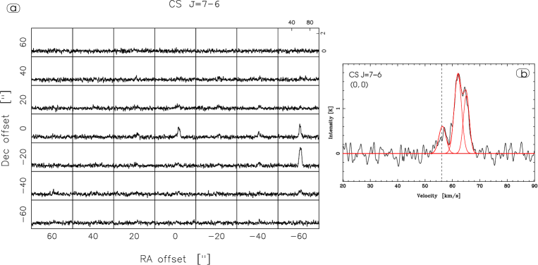
Figure 2: a)CS J=7–6 spectra obtained towards the 2^′ $\times$ 2^′ region (white box in Fig. 1-left) mapped with ASTE. b) Hanning smoothed profile of the CS J=7–6 line towards G45.47 at the position (0, 0). The dashed line indicates the systemic velocity of the gas. The spectrum was deconstructed using three Gaussians, which are shown in red.

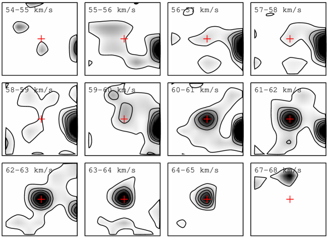
Figure 3: Velocity channel maps of the CS J=7-6 emission averaged every 1 km s^-1. Greyscale goes from 0.15 (about 3$\sigma$ rms noise of an averaged channel map) up to 1.8 K. Contours levels are at 0.15, 0.3, 0.45 and 0.6 K. The red cross represents the position of G45.47.

Figure 4-a shows the HCO⁺ J=4–3 spectra obtained towards the same region. As in the case of the CS J=7–6 spectrum it can be seen that the HCO⁺ emission towards (0, 0) can be deconstructed in three velocity components, a very weak one centered at about 56 km s^-1 (intensity of about 2$\sigma$), plus two brighter ones at 61 and 65 km s^-1, with only one dip centered at $\sim$ 63 km s^-1.

From Fig. 4-a it can be noticed that the HCO⁺ spectrum on position ($-$60, $-$20), that is at the position of the UCHII region G45.45, has also a dip at about 60 km s^-1 similarly to what it is observed in the CS J=7–6 line towards the same position.

The HCO⁺ spectra also show evidence of emission near position (60, $-$40). This molecular feature is in positional coincidence with an infrared (IR) source located at RA=19^h14^m27.7^s, dec.=+11^∘08^′33^′′(J2000) (see Fig 1). As this HCO⁺ spectrum has the same kinematic structure than the spectrum towards ($-$60, $-$20) including the presence of a dip at the same velocity of about 60 km s^-1, we can conclude that this IR source is embedded in a molecular filament that must be connected with G45.45.

Figure 5 shows the velocity channel maps of the HCO⁺ J=4–3 emission averaged every 1 km s^-1. The HCO⁺ J=4–3 emission related to G45.47 is visible between $\sim$ 55 and $\sim$ 68 km s^-1, while the emission associated with G45.45 goes from $\sim$ 54 to $\sim$ 63 km s^-1, respectively. Between $\sim$ 56 and $\sim$ 60 km s^-1part of the molecular condensation related to the IR source mentioned above can be appreciated.

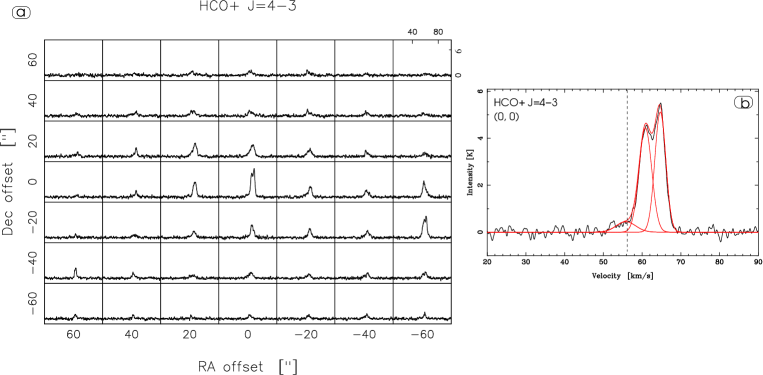
Figure 4: a) HCO⁺ J=4–3 spectra obtained towards the 2^′ $\times$ 2^′ region (white box in Fig. 1-left) mapped with ASTE. b) Hanning smoothed profile of the HCO⁺ J=4–3 line towards the position (0, 0) where it is G45.47. The dashed line indicates the systemic velocity of the gas. The spectrum was deconstructed using three Gaussians, which are shown in red.

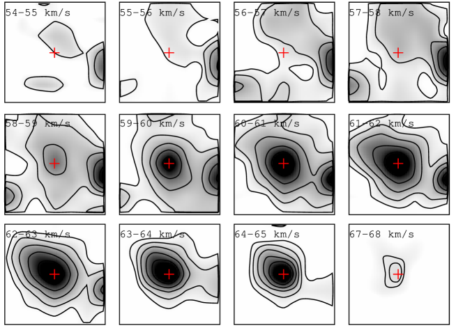
Figure 5: Velocity channel maps of the HCO⁺ J=4–3 emission averaged every 1 km s^-1. Greyscale goes from 0.15 (about 3$\sigma$ rms noise of an averaged channel map) to 2.5 K. Contours levels are at 0.15, 0.5, 0.8, 1.3, and 1.9 K. The red cross represents the position of G45.47.

Figure 6 shows the ¹³CO J=3–2 spectra towards the same region. The ¹³CO emission towards (0, 0) can be decomposed in three velocity components centered at about 56 (the systemic velocity of the gas), 60, and 63 km s^-1, while only one dip centered at $\sim$ 58 km s^-1can be appreciated. The depression at 58 km s^-1 can be observed in almost all the ¹³CO J=3–2 spectra in the region. Figure 7 shows the velocity channel maps of the ¹³CO J=3–2 emission averaged every 1 km s^-1.

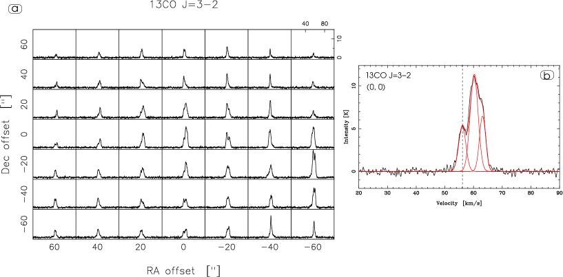
Figure 6: ¹³CO J=3–2 spectra obtained towards the 2^′ $\times$ 2^′ region (white box in Fig. 1-left) mapped with ASTE. b) Hanning smoothed profile of the ¹³CO J=3–2 line towards G45.47. The dashed line indicates the systemic velocity of the gas. The spectrum was deconstructed using three Gaussians, which are shown in red.

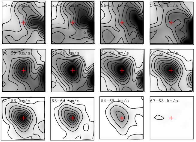
Figure 7: Velocity channel maps of the ¹³CO J=3–2 emission averaged every 1 km s^-1. Greyscale goes from 0.15 up to 9 K. Contours levels are at 0.6, 2, 4, 5, 6, 7, 8, and 9 K. The red cross represents the position of G45.47.

The ¹²CO J=3–2 spectra (Fig. 8) exhibit a more complicated behaviour. The profile towards the position (0, 0) has a triple peak structure with components centered at about 55, 60, and 64 km s^-1and two dips at about 58 and 62 km s^-1. This spectrum is broadened, suggesting the presence of outflowing activity in the region with the blue wing centered near the position (20, 20) and the red wing around the (0, $-$40) offset.

In Figure 9 we show the velocity channel maps of the ¹²CO J=3–2 emission averaged every 2.1 km s^-1. Among all the observed molecular condensations, we draw the attention onto the clumps related to G45.47 and G45.45. The molecular clump related to G45.47 is observed between $\sim$ 62 and 66 km s^-1and is seen slightly shifted to the northwest between $\sim$ 58 and 62 km s^-1. The clump associated with G45.45 (partially observed) is centered at RA=19^h14^m22^s, dec.=+11^∘09^′20^′′(J2000) in the velocity interval going from 47 to 63 km s^-1. Although both molecular condensations have associated different velocity ranges, they are connected through the extended emission shown in the velocity interval going from 50 to 65 km s^-1. The molecular gas related to the spectral wings appears as two conspicuous molecular features centered at RA=19^h14^m27^s, dec.=+11^∘09^′45^′′(J2000) between 35 and 53 km s^-1  and at RA=19^h14^m26^s, dec.=+11^∘08^′45^′′(J2000) between 65 and 76 km s^-1. These features will be further discussed in Section 3.3.

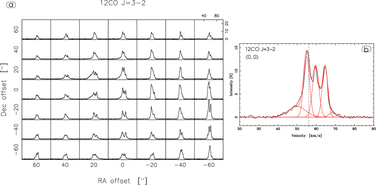
Figure 8: a) ¹²CO J=3–2 spectra obtained towards the 2^′ $\times$ 2^′ region (white box in Fig. 1-left) mapped with ASTE. b) Hanning smoothed profile of the ¹²CO J=3–2 line towards G45.47. The dashed line indicates the systemic velocity of the gas. The spectrum was deconstructed using five Gaussians, which are shown in red.

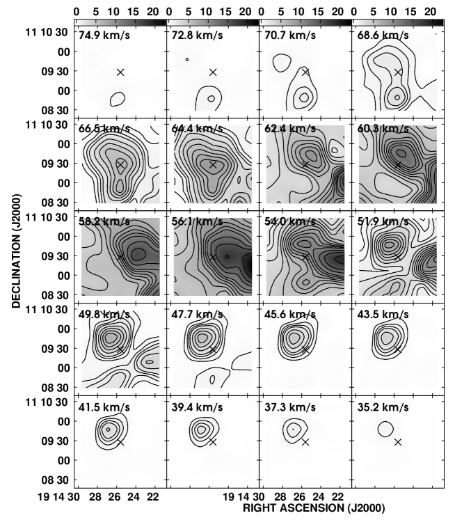
Figure 9: Velocity channel maps of the ¹²CO J=3–2 emission averaged every 2.1 km s^-1. The given velocities correspond to the higher velocity of each interval. Greyscale goes up to 23 K. Contours are above the 5$\sigma$ of the rms noise level. The cross indicates the position of G45.47.

The four transitions have, within errors, the same main velocity components at about 55, 60, and 64 km s^-1 towards the position (0, 0). By the other hand, the velocity components observed at about 51 and 68 km s^-1 in the ¹²CO J=3–2 spectrum are not detected in the other three lines. Table LABEL:gaussianfit lists the emission peaks parameters derived from a Gaussian fitting for the four molecular transitions on the position (0, 0). T_mb represents the peak brightness temperature and V_LSR the central velocity referred to the Local Standard of Rest. Errors are formal 1$\sigma$ value for the model of Gaussian line shape. All the spectra towards the (0,0) position have the same self-absorption dip at about 58-59 km s^-1, which correspond to the central velocity of the molecular cloud GRSMC 045.49+00.04 where G45.47 is embedded. Even more, this spectral feature is observed in all transitions towards the region G45.45 and the IR source located at RA=19^h14^m27.7^s, dec.=+11^∘08^′33^′′(J2000) (see Fig 1).

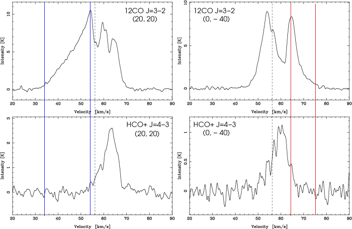
Figure 10: Comparison between the ¹²CO J=3–2 and the HCO⁺ J=4–3 spectra on the positions (20, 20) and (0, -40). The dashed line indicates the systemic velocity. The velocity intervals corresponding to the blue and red wings are shown. The four spectra were Hanning smoothed.

Table 1: Emission peaks parameters derived from a Gaussian fitting for the four molecular transitions spectra on the position (0, 0).

Transition	VLSR [km s-1]	Tmb [K]	$\Delta$v [km s-1]
CS J=7–6	56.3$\pm$0.9	0.6$\pm$0.2	3.1$\pm$0.6
	62.0$\pm$0.8	1.8$\pm$0.1	3.1$\pm$0.7
	64.8$\pm$1.1	1.3$\pm$0.1	2.5$\pm$0.9
HCO+ J=4–3	55.8$\pm$1.2	0.4$\pm$0.2	5.9$\pm$0.5
	60.8$\pm$1.4	4.4$\pm$0.8	3.8$\pm$0.6
	64.7$\pm$1.7	5.1$\pm$0.6	3.3$\pm$0.7
13CO J=3–2	55.9$\pm$0.6	5.2$\pm$0.4	2.9$\pm$0.4
	60.5$\pm$0.5	11.1$\pm$0.8	3.3$\pm$0.6
	63.3$\pm$0.4	6.4$\pm$0.7	2.6$\pm$0.7
12CO J=3–2	50.7$\pm$0.3	3.0$\pm$0.2	9.0$\pm$0.3
	55.2$\pm$0.1	13.1$\pm$1.1	3.3$\pm$0.4
	59.8$\pm$0.2	10.6$\pm$0.8	3.6$\pm$0.6
	64.4$\pm$0.6	10.6$\pm$0.7	3.3$\pm$0.5
	68.1$\pm$0.4	1.3$\pm$0.2	4.4$\pm$0.4

3.2 Column density and mass estimates of the molecular clump associated with G45.47

We estimate the ¹³CO J=3–2 opacity, $\tau_{13}$, based on the following equation:

$$\small\tau_{13}=-ln\left(1-\frac{T_{peak}(^{13}{\rm CO})}{T_{peak}(^{12}{\rm CO})}\right)$$ (1)

where we consider T_peak from the position (0, 0). We obtain, $\tau_{13}\sim$ 1.9 which reveals that the ¹³CO J=3–2 emission is optically thick towards G45.47, in agreement with the observed profile towards (0,0) offset (see Fig. 6).

The excitation temperature, $T_{ex}$, of the ¹³CO J=3–2 line was estimated from:

$$\small{}^{13}T_{peak}=\frac{h\nu}{k}\left(\frac{1}{e^{h\nu/kT_{ex}}-1}-\frac{1}{e^{h\nu/kT_{BG}}-1}\right)\times(1-e^{-\tau_{13}})$$ (2)

where for this line $h\nu/k=15.87$. Assuming $T_{BG}$ = 2.7 K, and considering the peak brightness temperature for the ¹³CO J=3–2 at (0, 0) offset, ${}^{13}T_{peak}$ = 11.15 K, we derive a $T_{ex}\sim$ 20 K for the ¹³CO J=3–2 line.

Finally, using the RADEX code (van der Tak et al., 2007) we derive the ¹³CO J=3–2 column density and the H₂ volume density. The RADEX model uses the mean escape probability approximation for the radiative transfer equation.

Adopting $T_{ex}\sim$ 20 K, $\tau_{13}\sim$ 1.9, and ${}^{13}T_{peak}$ = 11.15 K, we obtain a ¹³CO column density N(¹³CO) $\sim 2.8\times 10^{17}{\rm cm}^{-2}$ and n(H₂) $\sim 10^{5}{\rm cm}^{-3}$. Considering an abundance ratio of [H₂]/[¹³CO] = 77$\times 10^{4}$ (Wilson & Rood, 1994) we estimate the H₂ column density, N(H${}_{2})\sim 2.1\times 10^{23}{\rm cm}^{-2}$. Finally, using the relation $M=\mu m_{H}d^{2}\Omega{\rm N(H_{2})}$, where $\mu$ is the mean molecular weight per H₂ molecule ($\mu\sim 2.72$), $m_{H}$ the hydrogen atomic mass, $d$ the distance, and $\Omega$ the solid angle subtended by the structure, we calculate the total mass of the clump in $M\sim 10^{4}$ M_⊙.

As an independent estimate, we derive the beam-averaged gas column density, the mass, and the volume density of the clump based on the dust continuum emission. In particular, we use the integrated flux of the continuum emission at 1.1 mm as obtained from The Bolocam Galactic Plane Survey II Catalog (BGPS II; Rosolowsky et al. 2010). The 1.1 mm continuum emission is mostly originated in optically thin dust (Hildebrand, 1983). Following Beuther et al. (2002a) and Hildebrand (1983) we calculate the mass and the gas column density of the clump using:

$$M_{gas}=\frac{1.3\times 10^{-3}}{J_{\nu}(T_{dust})}\frac{a}{0.1\mu{\rm m}}\frac{\rho}{3{\rm gcm}^{-3}}\frac{R}{100}\frac{F_{\nu}}{{\rm Jy}}$$

$$\left(\frac{d}{{\rm kpc}}\right)^{2}\left(\frac{\nu}{2.4{\rm THz}}\right)^{-3-\beta}[{\rm M}_{\odot}]$$ (3)

and

$$N_{gas}=\frac{7.8\times 10^{10}}{J_{\nu}(T_{dust})\Omega_{b}}\frac{a}{0.1\mu{\rm m}}\frac{\rho}{3{\rm gcm}^{-3}}\frac{R}{100}\frac{F_{\nu}}{{\rm Jy}}$$

$$\left(\frac{\nu}{2.4{\rm THz}}\right)^{-3-\beta}[{\rm cm}^{-2}]$$ (4)

where $J_{\nu}(T_{dust}$) = [exp($h\nu/kT_{dust})-1]^{-1}$ and $\Omega_{b},a,\rho,R,$ and $\beta$ are the beam solid angle, grain size, grain mass density, gas-to-dust ratio, and grain emissivity index for which we used the values of (33^′′)² in radians, 0.1 $\mu$m, 3 g cm^-3, 100, and 2, respectively (Hunter 1997, Hunter et al. 2000, and Molinari et al. 2000). Based on the work of Sridharan et al. (2002) who derived dust temperatures ranging between 30 and 60 K for a sample of several massive star forming regions, we adopt $T_{dust}$ = 45 K. For a distance $d$ = 8.3 kpc and an integrated flux intensity $F_{\nu}$ = 5.18 Jy at 1 mm (Rosolowsky et al., 2010) we obtain $N_{gas}\sim 4\times 10^{23}$ cm^-2, $M_{gas}\sim 8520$ M_⊙, and a volume density, $n$(H${}_{2})\sim 1.4\times 10^{5}$ cm^-3. These values are in good agreement with those derived from the ¹³CO J=3–2 line using RADEX.

3.3 Molecular outflows associated with G45.47

As discussed in Section 3.1, the presence of spectral wings in the ¹²CO J=3–2 spectrum obtained towards G45.47 is a strong indicator that molecular outflow activity is taking place in the region. To characterize the associated molecular outflows it is first necessary to separate the outflowing gas from the molecular material of the clump, identifying the velocity ranges related to each structure.

We consider two independent methods to determine these velocity ranges. The first method consists in the identification of the blue and red spectral wings based on a comparison between the ¹²CO J=3–2 and HCO⁺ J=4–3 spectra. Figure 10 shows the comparison between both spectra on positions (20, 20) and (0, $-$40) where the blue and red wings are largest. Considering emission up to about 2 $\sigma$ of rms noise level, it can be noticed a blue and a red wing in the ¹²CO spectra between $\sim$ 34 and $\sim$ 54 and between $\sim$ 64 and $\sim$ 75 km s^-1, respectively.

The second method to identify the molecular outflows is based on the inspection of the ¹²CO J=3–2 data cube, channel by channel, trying to spatially separate both outflows’s lobes. In Section 3.1 we mentioned two molecular features in the ¹²CO J=3–2 emission centered at RA=19^h14^m27^s, dec.=+11^∘09^′45^′′(J2000) between $\sim$ 34 and $\sim$ 54 km s^-1 and at RA=19^h14^m26^s, dec.=+11^∘08^′45^′′(J2000) between $\sim$ 64 and $\sim$ 75 km s^-1 which we identify as the outflow’s lobes related to G45.47 (see Fig. 9). These molecular features can be identified as the spectral wings detected in the ¹²CO J=3–2 spectra through the first method. Figure 11 shows a Spitzer-IRAC three color image (3.6 $\mu$m = blue, 4.5 $\mu$m = green and 8 $\mu$m = red) of G45.47. The blue and red contours represent the ¹²CO J=3–2 emission integrated from $\sim$ 34 to 54 km s^-1 (blue lobe) and from $\sim$ 64 to 75 km s^-1 (red lobe), respectively.

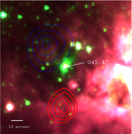
Figure 11: Spitzer-IRAC three color image (3.6 $\mu$m = blue, 4.5 $\mu$m = green and 8 $\mu$m = red) of G45.47. The blue and red contours represent the ¹²CO J=3–2 emission integrated from 34 to 54 km s^-1 (blue lobe), and from 64 to 75 km s^-1 (red lobe), respectively. The blue contours are at 400, 500, 600, and 670 K km s^-1  and the red ones are at 140, 160, 180, and 200 K km s^-1.

Following Scoville et al. (1986) we estimate the ¹²CO optical depth, $\tau_{12}$, of the gas in the molecular outflows using:

$$\small\frac{{}^{12}{\rm T}_{mb}}{{}^{13}{\rm T}_{mb}}=\frac{1-exp(-\tau_{12})}{1-exp(-\tau_{12}/X)}$$ (5)

where $X$=[¹²CO]/[¹³CO] is the isotope abundance ratio. Using the relation $X=6.21\times D_{GC}+18.71$ (Milam et al., 2005), where D_GC = 6.1 kpc is the distance between G45.47 and the Galactic Center, we obtain an isotope abundance ratio $X$= 57 for this region. We adopt a constant $X$ throughout the outflows (Cabrit & Bertout, 1990). Since we could not identify any blue wing in the ¹³CO spectrum on position (20, 20), the ¹²T${}_{mb}/^{13}$T_mb ratio for both wings was estimated considering only the red one. We obtain a ¹²T${}_{mb}/^{13}$T_mb ratio of about 4.2 and derive a ¹²CO optical depth of $\tau_{12}\sim$ 15, which will be adopted for both spectral wings in further calculations.

We can now estimate the ¹²CO column density of both outflow lobes from (see e.g. Buckle et al. 2010):

$$\small{\rm N}(^{12}{\rm CO})=7.96\times 10^{13}e^{\frac{16.6}{T_{ex}}}\frac{T_{ex}+0.92}{1-exp(\frac{-16.6}{T_{ex}})}\int\tau_{12}{\rm dv}$$ (6)

Taking into account that the ¹²CO J=3–2 is an optically thick transition ($\tau\geq 1$), the integral can be approximated by:

$$\small\int\tau_{12}{\rm dv}=\frac{1}{J(T_{ex})-J(T_{BG})}\frac{\tau_{12}}{1-e^{-\tau_{12}}}\int{\rm{}^{12}T}_{mb}\leavevmode\nobreak\ {\rm dv}$$ (7)

By integrating the ¹²CO emission from 34 to 54 km s^-1 and from 64 to 75 km s^-1 we obtain N(CO)${}_{blue}\sim 5.2\times 10^{17}{\rm cm}^{-2}$ and N(CO)${}_{red}\sim 2\times 10^{17}{\rm cm}^{-2}$, respectively. The mass of each wing can be derived from the relation $M=\mu m_{H}d^{2}\Omega X({\rm CO})^{-1}{\rm N(CO)}$, where $X$(CO) is the ¹²CO relative abundance to H₂ ($X$(CO)$\sim 7.4\times 10^{-5}$). We obtain M${}_{blue}\sim 300$ M_⊙ and M${}_{red}\sim 120$ M_⊙, yielding a total outflow mass of about 420 M_⊙. In this way, the estimated total outflows mass represents about 4% of the clump mass, which is in agreement with the results of Beuther (2002b) who established that approximately 4% of the clump gas is entrained in the molecular outflows.

The momentum and the kinetic energy of the wings can be derived from $P=MV_{c}$ and $E_{k}=0.5MV_{c}^{2}$, where $V_{c}$ is a characteristic velocity estimated as the difference between the maximum velocity of detectable ¹²CO emission in the wing and the systemic velocity of the gas ($\sim$ 56 km s^-1). Taking into account a $V_{c}^{blue}\sim$ 22 km s^-1  and a $V_{c}^{red}\sim$ 19 km s^-1, we obtain $P_{blue}=6.6\times 10^{3}$ M_⊙km s^-1, $P_{red}=2.3\times 10^{3}$ M_⊙km s^-1, $E_{k}^{blue}=1.4\times 10^{48}$ erg and $E_{k}^{red}=4.2\times 10^{47}$ erg. Comparing our results with the work of Wu et al. (2004) who based on compiled data concluded that the mass, momentum, and energy of molecular outflows range from 10^-3 to 10³ M_⊙, 10^-3 to 10⁴ M_⊙km s^-1 and 10³⁸ to 10⁴⁸ erg, respectively, we can infer that in this work we are dealing with massive and energetic outflows.

Following Curtis et al. (2010) we define the dynamical time for the blue and red wings, $t_{dyn}$, as the time for the bow shock travelling at the maximum velocity in the flow, $V_{c}$, to travel the projected lobe length, $R_{lobe}$:

$$t_{dyn}=\frac{R_{lobe}}{V_{c}}$$ (8)

with $R_{lobe}^{blue}$ = 1.8 pc and $R_{lobe}^{red}$ = 1.6 pc. These values were obtained by inspecting the blue and red lobe sizes in Fig. 11 and considering a distance of 8.3 kpc. We obtain a similar dynamical time of both lobes, $t_{dyn}=0.8\times 10^{5}$ yr. According to Beuther et al. (2002b), flow ages are good estimates of protostar lifetimes. We can then assume that the protostar responsible of the outflow activity has an age of the order of $10^{5}$ yr. This is consistent with the detection of ionized gas in the region, since to be able to ionize its surroundings the age of the protostar should be at least $10^{5}$ yr (Sridharan et al., 2002).

3.4 HCO⁺ as tracer of molecular outflows

As an independent test of out findings, we performed a study of the HCO⁺ abundance towards G45.47. HCO⁺ is believed to be the dominant ionized species in dense dark clouds (Rawlings et al., 2000; Dalgarno & Lepp, 1984), being very important for the ion-neutral chemistry. The ionization fraction of molecular clouds is a relevant parameter to study the cloud chemistry and dynamics, and hence the star forming processes. Star formation occurs in the interior of dense cores, regions of high extinction where self-shielding prevents the UV photoionization of H₂. Thus, cosmic ray ionization is believed to dominate photoionization in dense cores (McKee, 1989). However, when YSOs are formed within the cores, the shocks and outflows produce deep changes in the chemistry and photoionization processes are very likely. Indeed, in star forming regions occur a molecular enrichment due to the desorption of molecular-rich ice mantles, followed by photochemical processing by shock-generated radiation fields. In particular, towards YSOs which are driving outflows, it is expectable an enhancement in the HCO⁺ abundance (Rawlings et al., 2000, 2004). In what follows, we estimate, using a simple chemical network, the HCO⁺ abundance that would be produced by an standard cosmic ray ionization rate in the G45 clump in order to compare with the abundance obtained from our observations.

The starting chemical reaction to form HCO⁺ is the production of H${}_{3}^{+}$, mainly formed in the interaction between the cosmic rays (c.r.) and the molecular gas (e.g. Oka 2006):

$$\centering{\rm H_{2}+c.r.}\@add@centering \rightarrow {\rm H_{2}^{+}+e^{-}}$$

$${\rm H_{2}^{+}+H_{2}} \rightarrow {\rm H_{3}^{+}+H.}$$ (9)

The rate equation of this reaction is

$$\zeta_{\rm H_{2}}\leavevmode\nobreak\ n({\rm H_{2}})=\frac{dn({\rm H_{3}^{+}})}{dt},$$ (10)

where $\zeta_{\rm H_{2}}$ is the cosmic ray ionization rate and $n$ the density of the molecular species. By considering that the HCO⁺ is mainly formed by the reaction of H${}_{3}^{+}$ with CO:

$${\rm H_{3}^{+}+CO\rightarrow HCO^{+}+H_{2}}$$ (11)

and destroyed through recombination with electrons,

$${\rm HCO^{+}+e^{-}\rightarrow CO+H,}$$ (12)

the rate equations can be equated, leading to

$$k_{\rm HCO^{+}}\leavevmode\nobreak\ n({\rm H_{3}^{+}})\leavevmode\nobreak\ n({\rm CO})=k_{\rm CO}\leavevmode\nobreak\ n({\rm HCO^{+}})\leavevmode\nobreak\ n(e),$$ (13)

where $k_{\rm HCO^{+}}$ and $k_{\rm CO}$ are the coefficient rates and $n(e)$ the electron density. Assuming that the main destruction mechanism for H${}_{3}^{+}$ is through the formation of HCO⁺, the rate of destruction of H${}_{3}^{+}$ is therefore equal to the formation rate of HCO⁺; this implies that the left side of equation (10) is equal to right side of equation (13). Then, it is possible to write an expression for the cosmic ionization rate as a function of the molecular densities:

$$\zeta_{\rm H_{2}}=k_{\rm CO}\frac{n({\rm HCO^{+}})\leavevmode\nobreak\ n(e)}{n({\rm H_{2}})}.$$ (14)

The rate coefficient $k_{\rm CO}$, extracted from the UMIST database (Woodall et al., 2007), is: $k_{\rm CO}=2.4\times 10^{-7}(T/300{\rm K})^{-0.69}$. Equation (14) can be approximated using the column densities, leading:

$$\zeta_{\rm H_{2}}\simeq k_{\rm CO}\frac{{\rm N(HCO^{+})}\leavevmode\nobreak\ X(e)\leavevmode\nobreak\ n({\rm H_{2}})}{\rm N(H_{2})},$$ (15)

where $X(e)$ is the electron abundance. Using this equation and assuming typical values for the cosmic ionization rate and electron abundance of $\zeta_{\rm H_{2}}=(1-5)\times 10^{-17}$ s^-1 (Dalgarno, 2006) and $X(e)\sim 10^{-7}$ (Bergin et al., 1999), respectively, we derive the HCO⁺ column density. We use N(H₂) $=2\times 10^{23}$ cm^-2 and $n({\rm H_{2}})=1\times 10^{5}$ cm^-3, as derived above, and we assume $T=20$ K. Finally, we obtain that the N(HCO⁺) should be in the range $(1.5-6.5)\times 10^{14}$ cm^-2, leading to an abundance $X({\rm HCO^{+}})$ in between $6.5\times 10^{-10}$ and $3.2\times 10^{-9}$.

On the other hand, we analyze the central HCO⁺ J=4–3 spectrum and use the RADEX code (van der Tak et al., 2007) to derive its column density. Assuming background and kinetic temperatures of 2.73 K and 20 K, respectively, and the same H₂ density used above, we varied the HCO⁺ column density until obtaining a good fit for the observed peak temperature. The best fit was obtained with N(HCO⁺)$\sim 1.5\times 10^{15}$ cm^-2, leading an abundance of $X({\rm HCO^{+}})\sim 7.5\times 10^{-9}$. This value, more than twice greater than the lager value obtained above, might indicate that the cosmic ray ionization is insufficient to produce the observed HCO⁺ abundance through the described chemical network. Therefore, following Rawlings et al. (2000, 2004), we suggest that the observed HCO⁺ abundance must be mostly produced by the outflowing activity in the region. In spite of the uncertainties in the calculations, this is an independent proof pointing to support an scenario with outflows in the region.

3.5 Looking for the driving source of the molecular outflows

Wilner et al. (1996) reported 5^′′ resolution observations of the HCO⁺ J=1–0 transition towards G45.47 obtained with the OVRO millimeter array. They identified at least five HCO⁺ J=1–0 clumps and suggested that the formation of an OB cluster would be taking place in the region. However the authors did not carry out any search of infrared point sources in the region to confirm that hypothesis. In this context, we wonder if the massive molecular outflows observed towards G45.47 were originated by one or more stars. Based on a near-infrared analysis, we searched for the driving source candidates of the massive molecular outflows.

Figure 12 shows the radio continuum emission at 6 cm obtained from The Multi-Array Galactic Plane Imaging Survey (MAGPIS; White et al. 2005) of the area mapped using ASTE. The green contours represent the HCO⁺ J=4–3 emission distribution integrated between 58 and 67 km s^-1. The black contours were taken from the paper of Wilner et al. (1996) and represent the HCO⁺ J=1–0 emission distribution integrated in the same velocity interval. The region observed by Wilner et al. (1996) is indicated by the dashed box. The five clumps reported by the authors have been labeled. The positional coincidence among the center of the HCO⁺ J=4–3 clump, the clump 3 of HCO⁺ J=1–0 and a radio continuum source, which has been identified as the UCHII region G45.47, is striking. The red circles indicate the location of the YSO candidates in the observed region (see red circles in Fig. 13). Among the five YSO candidates projected onto the HCO⁺ J=4–3 emission, 2MASS 19142564+1109283 is the only one having a positional coincidence with a clump of HCO⁺ J=1–0 (clump 3). We do not find any embedded infrared sources in the others four clumps, suggesting that these clumps could be in a prestellar core stage or they might be tracing the origin of the molecular outflows. We suggest that the most likely candidate to be the driving source of the molecular outflows is 2MASS 19142564+1109283.

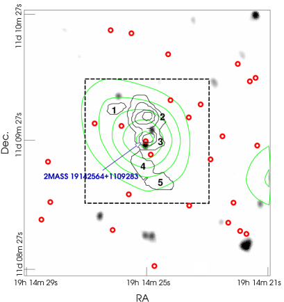
Figure 12: Radio continuum emission at 6 cm (MAGPIS; White et al. 2005) of the area mapped using ASTE. The green contours represent the HCO⁺ J=4–3 emission distribution integrated between 58 and 67 km s^-1. The black contours were taken from the paper of Wilner et al. (1996) and represent the HCO⁺ J=1–0 emission distribution integrated from 58 and 67 km s^-1. The box indicates the area observed by Wilner et al. (1996). The numbers show the five HCO⁺ J=1–0 clumps. The red circles represent the YSO candidates shown in Fig. 13.

Figure 13 shows a color-color diagram (CCD) including all the 2MASS point sources located in the observed region. The red circles represent the sources with infrared excess (YSO candidates) which have been shown in Figure 12. The reddenest object is 2MASS 19142564+1109283. The blue circles represent main sequence or giant star candidates.

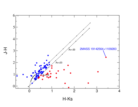
Figure 13: Color-color diagram of the 2MASS infrared sources in the vicinity of G45.47. The two solid curves represent the location of the main sequence (thin line) and the giant stars (thick line) derived from Bessell & Brett (1988). The parallel dashed lines are reddening vectors with the crosses placed at intervals corresponding to five magnitudes of visual extinction. We have assumed the interstellar reddening law of Rieke & Lebofsky (1985) (A_J/A_V =0.282; A_H/A_V =0.175 and A_K/A_V =0.112). The sources reddened by circumstellar dust are indicated as red circles.

To characterize the infrared source 2MASS 19142564+1109283 we perform a fitting of its spectral energy distribution (SED) using the tool developed by Robitaille et al. (2007). We adopt an interstellar extinction in the line of sight, A_v, between 5 and 17 magnitudes. The range of A_v was chosen by inspecting the location in a [H-K] vs [J-H] CCD of the 2MASS sources in the region (see Fig. 13). To construct the SED we consider the fluxes at the JHK 2MASS bands, Spitzer-IRAC 5.8 and 8 $\mu$m bands, WISE 3.4, 4.6, 12 and 22 $\mu$m bands, MSX 14 and 21 $\mu$m bands, and SCUBA 850 $\mu$m band. The fluxes of the datasets having lower angular resolution (MSX and SCUBA) were considered as upper limits. Figure 14 shows the best fitting SEDs models for 2MASS 19142564+1109283. We select models that satisfies the condition:

$$\chi^{2}-\chi_{best}^{2}<2N,$$ (16)

where $\chi_{best}^{2}$ is the minimum value of the $\chi^{2}$ among all models, and $N$ is the number of input data fluxes (fluxes specified as upper limit do not contribute to $N$). Hereafter, we refer to models satisfying Eq. 16 as “selected models”.

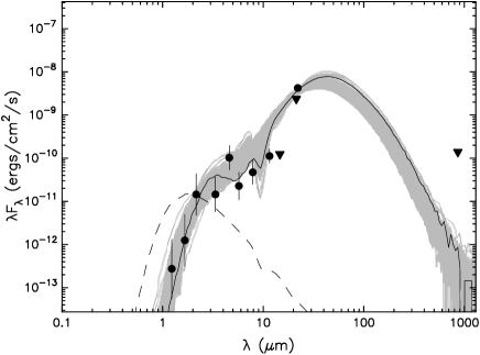
Figure 14: Best fitting SED models for G45.47. The fill circles indicate the measured fluxes at the JHK 2MASS bands, Spitzer-IRAC bands at 5.8 and 8.0 $\mu$m, and the WISE bands at 3.4, 4.6, 12 and 22 $\mu$m. Triangles indicate fluxes considered as upper limits, as MSX bands at 14 and 21 $\mu$m and the SCUBA band at 850 $\mu$m. Black and gray solid curves represent the best-fit model and the subsequent good fittings, respectively. The dashed line shows the best-fit model for a central source contribution in absence of circumstellar dust.

From the SED fitting several model parameters can be obtained and, as expected, some can be better constrained than others. Taking into account the values yielding by the “selected models” for several parameters, we derive the following main results:

• the total luminosity distribution of the source has an average value of $2\times 10^{4}$ L_⊙ with a spread between $8\times 10^{3}$ and $5\times 10^{4}$ L_⊙.

• embedded in the molecular clump there is a massive protostar of about 15 M_⊙ (early B-type star) accreting material from its envelope at large rates, $\dot{M}_{env}\sim 2\times 10^{-4}$ M_⊙ yr^-1.

• despite the large spread in the central source’s age distribution that goes from $2\times 10^{3}$ to $10^{6}$ yr, it peaks at about $3\times 10^{5}$ yr, as expected for protostars that has begun to ionize their surroundings. Besides, this result is in agreement with the dynamical time, $t_{dyn}=1\times 10^{5}$ yr, derived in Section 3.3.

4 Summary

We carried out a study of the UCHII region G045.47+0.05 and its surroundings based on molecular lines observations and public infrared data. We find a molecular gas condensation associated with G045.47+0.05. The detection of the CS J=7–6 transition reveals that the UCHII region is still embedded in warm and dense molecular gas. The CS spectrum obtained towards the position (0, 0) has a pronounced self-absorption dip at about 59 km s^-1with the red velocity component more intense than the blue one. This asymmetry in the CS profile suggests an expansion of the molecular gas.

All molecular transitions have the same main three velocity components with a self-absorption dip at about 58-59 km s^-1which correspond to the central velocity of the molecular cloud GRSMC G045.49+00.04 where G45.47 is embedded.

Based on the ratio between the ¹²CO and ¹³CO J=3-2 transitions we estimate the ¹³CO opacity, $\tau_{13}$, towards the center of the clump in about 1.9, revealing that this line is optically thick. This result is in agreement with the structure exhibited by the ¹³CO spectrum towards the center of G045.47+0.05.

Using the RADEX code we derive a ¹³CO J=3-2 column density and H₂ volume density of about $2.8\times 10^{17}$ cm^-2 and 10⁵ cm^-3, respectively. The H₂ column density and the total mass of the clump were estimated in $2.1\times 10^{23}$ cm^-2 and $M\sim 10^{4}$ M_⊙, respectively.

From an independent estimate based on the dust continuum emission at 1 mm we derive $N_{gas}\sim 4\times 10^{23}$ cm^-2, $M_{gas}\sim 8520$ M_⊙, and a volume density, $n$(H${}_{2})\sim 1.4\times 10^{5}$ cm^-3, in good agreement with the values derived from the molecular lines.

From the analysis of the ¹²CO J=3-2 and HCO⁺ transitions we report the presence of molecular outflows related to the UCHII region G045.47+0.05. We estimate the blue and red lobes masses in about 300 and 120 M_⊙, respectively. The total mass of the outflows represents about 4% of the clump mass. The dynamical time of both lobes, good indicator of the protostar age, was estimated in about $8\times 10^{4}$ yr. This agrees with the presence of ionized gas around the central object.

Based on infrared data we searched for the protostar(s) that must be driving the outflows. We find that the source 2MASS 19142564+1109283 is a YSO candidate located onto the center of the clump in coincidence with the radio continuum emission associated with the UCHII region. Besides this infrared source is the only YSO candidate related to one of the five HCO⁺ clump detected by Wilner et al. (1996). We did not detected any YSO candidate associated with the other four HCO⁺ clumps. This results suggests that the massive molecular outflows are generated by the protostar 2MASS 19142564+1109283.

Finally, from a spectral energy distribution analysis of the source we derive a total luminosity, a protostar’s mass, and protostar’s age of about $2\times 10^{4}$L_⊙, 15 M_⊙(early B-type star), and $3\times 10^{5}$ yr, respectively.

Massive molecular outflows give, on large scales, a good piece of information about the physical processes taking place in the innermost parts of the star-forming cores. Their detection give indirect evidence that massive star formation is a scaled-up version of low mass star formation. The identification of a massive protostar that would be generating the massive outflows reinforces this scenario.

References

- Bergin et al. (1999) Bergin, E. A., Plume, R., Williams, J. P., & Myers, P. C. 1999, ApJ, 512, 724
- Bessell & Brett (1988) Bessell, M. S. & Brett, J. M. 1988, PASP, 100, 1134
- Beuther (2002a) Beuther, H. 2002a, PhD thesis, Max-Planck-Institut für Radioastronomie
- Beuther (2002b) Beuther, H. 2002b, PhD thesis, Max-Planck-Institut für Radioastronomie
- Beuther et al. (2002a) Beuther, H., Schilke, P., Menten, K. M., et al. 2002a, ApJ, 566, 945
- Beuther et al. (2002b) Beuther, H., Schilke, P., Sridharan, T. K., et al. 2002b, A&A, 383, 892
- Bonnell & Bate (2006) Bonnell, I. A. & Bate, M. R. 2006, MNRAS, 370, 488
- Buckle et al. (2010) Buckle, J. V., Curtis, E. I., Roberts, J. F., et al. 2010, MNRAS, 401, 204
- Cabrit & Bertout (1990) Cabrit, S. & Bertout, C. 1990, ApJ, 348, 530
- Caswell et al. (1995) Caswell, J. L., Vaile, R. A., Ellingsen, S. P., Whiteoak, J. B., & Norris, R. P. 1995, MNRAS, 272, 96
- Curtis et al. (2010) Curtis, E. I., Richer, J. S., Swift, J. J., & Williams, J. P. 2010, MNRAS, 408, 1516
- Cyganowski et al. (2009) Cyganowski, C. J., Brogan, C. L., Hunter, T. R., & Churchwell, E. 2009, ApJ, 702, 1615
- Cyganowski et al. (2008) Cyganowski, C. J., Whitney, B. A., Holden, E., et al. 2008, AJ, 136, 2391
- Dalgarno (2006) Dalgarno, A. 2006, Proceedings of the National Academy of Science, 1031, 12269
- Dalgarno & Lepp (1984) Dalgarno, A. & Lepp, S. 1984, ApJ, 287, L47
- Ezawa et al. (2004) Ezawa, H., Kawabe, R., Kohno, K., & Yamamoto, S. 2004, in Society of Photo-Optical Instrumentation Engineers (SPIE) Conference Series, Vol. 5489, Society of Photo-Optical Instrumentation Engineers (SPIE) Conference Series, ed. J. M. Oschmann Jr., 763–772
- Fazio et al. (2004) Fazio, G. G., Hora, J. L., Allen, L. E., et al. 2004, ApJS, 154, 10
- Giveon et al. (2005a) Giveon, U., Becker, R. H., Helfand, D. J., & White, R. L. 2005a, AJ, 129, 348
- Giveon et al. (2005b) Giveon, U., Becker, R. H., Helfand, D. J., & White, R. L. 2005b, AJ, 130, 156
- Hildebrand (1983) Hildebrand, R. H. 1983, QJRAS, 24, 267
- Hiramatsu et al. (2007) Hiramatsu, M., Hayakawa, T., Tatematsu, K., et al. 2007, ApJ, 664, 964
- Hofner et al. (1999) Hofner, P., Peterson, S., & Cesaroni, R. 1999, ApJ, 514, 899
- Hunter (1997) Hunter, T. R. 1997, PhD thesis, Smithsonian Astrophysical Observatory, 60 Garden St. MS-78, Cambridge, MA 02178, USA
- Hunter et al. (2000) Hunter, T. R., Churchwell, E., Watson, C., et al. 2000, AJ, 119, 2711
- Hunter et al. (1997) Hunter, T. R., Phillips, T. G., & Menten, K. M. 1997, ApJ, 478, 283
- Kuchar & Bania (1994) Kuchar, T. A. & Bania, T. M. 1994, ApJ, 436, 117
- Lehtinen (1997) Lehtinen, K. 1997, A&A, 317, L5
- Leung (1978) Leung, C. M. 1978, ApJ, 225, 427
- Matthews et al. (1977) Matthews, H. E., Goss, W. M., Winnberg, A., & Habing, H. J. 1977, A&A, 61, 261
- McKee (1989) McKee, C. F. 1989, ApJ, 345, 782
- Milam et al. (2005) Milam, S. N., Savage, C., Brewster, M. A., Ziurys, L. M., & Wyckoff, S. 2005, ApJ, 634, 1126
- Molinari et al. (2000) Molinari, S., Brand, J., Cesaroni, R., & Palla, F. 2000, A&A, 355, 617
- Oka (2006) Oka, T. 2006, Proceedings of the National Academy of Science, 1031, 12235
- Paron et al. (2009) Paron, S., Ortega, M. E., Rubio, M., & Dubner, G. 2009, A&A, 498, 445
- Peretto & Fuller (2009) Peretto, N. & Fuller, G. A. 2009, A&A, 505, 405
- Qin et al. (2008) Qin, S.-L., Wang, J.-J., Zhao, G., Miller, M., & Zhao, J.-H. 2008, A&A, 484, 361
- Rathborne et al. (2006) Rathborne, J. M., Jackson, J. M., & Simon, R. 2006, ApJ, 641, 389
- Rathborne et al. (2009) Rathborne, J. M., Johnson, A. M., Jackson, J. M., Shah, R. Y., & Simon, R. 2009, ApJS, 182, 131
- Rawlings et al. (2004) Rawlings, J. M. C., Redman, M. P., Keto, E., & Williams, D. A. 2004, MNRAS, 351, 1054
- Rawlings et al. (2000) Rawlings, J. M. C., Taylor, S. D., & Williams, D. A. 2000, MNRAS, 313, 461
- Rieke & Lebofsky (1985) Rieke, G. H. & Lebofsky, M. J. 1985, ApJ, 288, 618
- Robitaille et al. (2007) Robitaille, T. P., Whitney, B. A., Indebetouw, R., & Wood, K. 2007, ApJS, 169, 328
- Rosolowsky et al. (2010) Rosolowsky, E., Dunham, M. K., Ginsburg, A., et al. 2010, ApJS, 188, 123
- Scoville et al. (1986) Scoville, N. Z., Sargent, A. I., Sanders, D. B., et al. 1986, ApJ, 303, 416
- Sridharan et al. (2002) Sridharan, T. K., Beuther, H., Schilke, P., Menten, K. M., & Wyrowski, F. 2002, ApJ, 566, 931
- Tan & McKee (2002) Tan, J. C. & McKee, C. F. 2002, in Astronomical Society of the Pacific Conference Series, Vol. 267, Hot Star Workshop III: The Earliest Phases of Massive Star Birth, ed. P. Crowther, 267
- van der Tak et al. (2007) van der Tak, F. F. S., Black, J. H., Schöier, F. L., Jansen, D. J., & van Dishoeck, E. F. 2007, A&A, 468, 627
- White et al. (2005) White, R. L., Becker, R. H., & Helfand, D. J. 2005, AJ, 130, 586
- Wilner et al. (1996) Wilner, D. J., Ho, P. T. P., & Zhang, Q. 1996, ApJ, 462, 339
- Wilson & Rood (1994) Wilson, T. L. & Rood, R. 1994, ARA&A, 32, 191
- Wood & Churchwell (1989) Wood, D. O. S. & Churchwell, E. 1989, ApJS, 69, 831
- Woodall et al. (2007) Woodall, J., Agúndez, M., Markwick-Kemper, A. J., & Millar, T. J. 2007, A&A, 466, 1197
- Wu et al. (2004) Wu, Y., Wei, Y., Zhao, M., et al. 2004, A&A, 426, 503
- Zhou (1992) Zhou, S. 1992, ApJ, 394, 204