Hedging Swing contract on gas market

1 Introduction

Swing options on the gas market are american style option where daily quantities exercices are constrained and global quantities exerciced each year constrained too. The option holder has to decide each day how much he consumes of the quantities satisfying the constraints and tries to use a strategy in order to maximize its expected profit. Based on the indexation principle, the pay off fonction is a spread between the spot gas market and the value of an index composed of the past average of some commodities’ spot or future prices. Most of the time the commodities involved are gas and oil.
When the index is a fixed one (then it is a strike), the valuation of Swing option is a classical problem solved by dynamic programming. In order to implement the dynamic programming method , first trinomial trees were used jaillet1 to estimate conditional expectation, then Longstaff Schwartz method long2001 using regression and Partial Differential Equation methods wihlem .
At the opposite, Swing options on the gas market are very high dimensional problems due to the index definition. This problem can be linked to the problem of pricing moving average american options. These moving averaging options with early exercice features have been studing in broadie , Dai , grau . A common approach (see broadie ) is to use least square Monte Carlo to estimate conditional expectation in Montecarlo algorithm. Recently bernhart derived a new methodology based on exponentially weighted Laguerre polynomials expansion to approximate the moving average processes. The methodology developped is efficient but numerical results showed that the usual regression method regressing on both the gas price and the index value is accurate enough.
If the question of the valuation of these contracts is rather well explored, the hedge of such a contract has never been studied. Most of the time practionners just hedge the gaz spot component in the index ignoring the stochasticity of the index. Besides when practionners want to simulate the portfolio risk they have to include the dynamic hedge they plan for next years in order to assess their risk accurately. As for gas storage, a methodology based on tangent process has been developped by warin to evaluate the Delta and follow the hedging strategy. The mathematical proof of this approach based on the Danskin’s theorem is given in bonnans . In this paper the methodology based on the tangent forward method calculated during a dynamic programming algorithm is developped for the gas Swing options. Its accuracy is tested on a realistic contract where:

• prices follow a two factor model (see for example schwarz ),

• hedging products available are day ahead products till the end of the week, week ahead products till the end of the month, and monthly contract as they can be found at Henry Hub.

The efficiency of the hedge and the accuracy of the calculations are studied depending on :

• the regressor used to calculate conditional expectation,

• the products involved in the index that we decide to hedge,

• the frequency of the hedge with respect to the products involved in the index including exchange rates.

In the sequel we suppose that conditional expectation are calculated by the Longstaff-Schwartz method long2001 adapted with local functions as explained in bouchardwarin .
In the next section 2, the contract and the price model are described. In the following section 3, the methodology used to simulate the dynamic hedging is explained. Next numerical results are given and a concluding section 5 gives some recommandations in particular in terms of frequency of the dynamic hedging and the components to hedge.

2 The contract and the price modelization

2.1 The contract

The Swing contract is first characterized by the quantities that can be purshased. Daily exercice dates are given in days from $t_{start}$ to $t_{end}$. Each day $t$ the option holder can exercise a quantity $q_{t}$ satisfying

$$0\leq q_{t}\leq q_{max}$$

Moreover the global quantity consummed $Q_{t}$ is constrained

$$Q_{min}\leq\sum_{t_{start}\leq t\leq t_{end}}q_{t}\leq Q_{max}.$$

The unitary pay off (for a quantity one) is given at a day $t$ by

$$S_{t}^{0}-I_{t}$$

where $S_{t}^{0}$ is the gas price and $I_{t}$ an index constant on each interval $[T_{i},T_{i+1}[$ where $T_{i}$ ($i=0$ to $\hat{n}$) are update dates defined in the contract. These dates correspond to the beginning of some months and typical values for $T_{i}$ are first day of each month, or first day of every two or three months.
For each exercice day $i$, we note $k(i)=\max\{j,T_{j}\leq i\}$. In the case of an additive index, the structure of the index for each exercice day $i$ is defined by the affine sum of $N$ components by :

$$I_{i}=I_{T_{k(i)}}=a_{0}+\sum_{j=1}^{N}a_{j}({\hat{S^{j}}}^{\tilde{l}(k(i)),\tilde{m}(k(i))}_{T_{k(i)}}-b_{j})X^{j}_{T_{k(i)}}$$

where :

• $\hat{S^{j}}^{\tilde{l},\tilde{m}}_{T}=\frac{1}{\tilde{m}}\sum_{q=1}^{\tilde{m}}S^{j}_{T-\tilde{l}-q}$ is the average of commodity $j$ (potentially a forward price) on the $\tilde{m}$ months expressed in days preceding the lag corresponding to $\tilde{l}$ months expressed in days involved in the index valid from date $T$ (see figure 1),

• $X^{j}_{T_{k}}$ is the exchange rate between the domestic currency and the foreign currency of the commodity $j$ at date $T_{k}$,

• $a_{j}$, $j=0...N$, $b_{j}=1,...N$ are coefficients given by the contract.

Remark 1

In some simple cases the lag and averaging windows are the same for each component of the index and the contract windows can be decribed by the triplet $m,l,p$ where $p$ gives in months the validity period for the index, $l$ the lag periode and $m$ the averaging window length.

Remark 2

In the formula, the exchange rates involved could be imposed by the contract at date $T(k)-\tilde{l}(k)$ or an average of the exchange rate could be imposed.

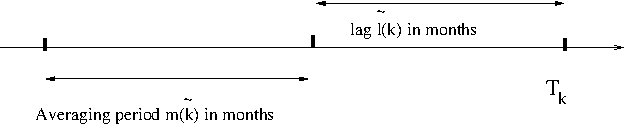
Figure 1: Lag and averaging windows for $\hat{S}^{\tilde{l}(k),\tilde{m}(k)}_{T_{k(i)}}$ calculation

2.2 Price Models

All over this section, we shall consider a $\tilde{n}$-dimensional Brownian motion $\left\{z^{1},\ldots,z^{\tilde{n}}\right\}$ with correlation matrix $\rho$ on a probability space $(\Omega,{\cal F},{\mathbb{P}})$ endowed with the natural (completed and right-continuous) filtration ${\mathbb{F}}=({\cal F}_{t})_{t\leq T}$ generated by $\left\{z^{1},\ldots,z^{\tilde{n}}\right\}$ up to some fixed time horizon $T>0$. The $\tilde{n}$ value will depend on the different models used for commodity prices and exchange rates.

Future Price Model

We suppose that the uncertainties in the commodity prices $S^{j}_{t}$, $j=0,N$ follows under the risk neutral measure a $\tilde{n}$-dimensional Ornstein-Uhlenbeck process. The following SDE describes our uncertainty model for the forward curve $F^{j}(t,T)$ giving the prices of a unitary amount of a commodity $j$ at day $t$ for delivery at date $T$ ( see clewlow ):

$$\frac{dF^{j}(t,T)}{F^{j}(t,T)}=\sum_{i=1}^{n}\sigma_{i}^{j}(t)e^{-a_{i}^{j}(T-t)}dz^{jn+i}_{t},\\$$ (1)

with $\sigma_{i}^{j}$ some volatility parameters and $a_{i}^{j}$ mean reverting parameters for commodity $j$.

Remark 3

Most of the time a two factors model is used. In this model, the first Brownian motion describes swift changes in the future curve, the second one describes structural changes in the gas market and deals with long term changes in the curve. The mean reverting parameter is generally taken equal to zero for the second term.

With the following notations:

$$V^{j}(t_{1},t_{2}) = \displaystyle{\int_{0}^{t_{1}}}\left\{\sum_{i=1}^{n}\sigma_{i}^{j}(u)^{2}e^{-2a_{i}^{j}(t_{2}-u)}+\right.$$

$$\left.2\sum_{i=1}^{n}\sum_{k=i+1}^{n}\rho_{i+jn,k+jn}\sigma_{i}^{j}(u)e^{-a_{i}^{j}(t_{2}-u)}\sigma_{k}^{j}(u)e^{-a_{k}^{j}(t_{2}-u)}\right\}du,$$

$$W^{i,j}_{t} = \displaystyle{\int_{0}^{t}}\sigma_{i}^{j}(u)e^{-a_{i}^{j}(t-u)}dz^{i+jn}_{u},\mbox{ for }i=1,\ldots,n$$

the integration of equation (1) gives :

$$F^{j}(t,T)=F^{j}(t_{0},T)e^{-\displaystyle{\frac{1}{2}}V^{j}(t,T)+\sum_{i=1}^{n}e^{-a_{i}^{j}(T-t)}W^{i,j}_{t}}.$$ (2)

With this modelization, the spot price for commodity $j$ is defined as the limit of the future price :

$$S^{j}_{t}=\lim_{T\downarrow t}F^{j}(t,T).$$ (3)

As for the instantaneous exchange rate for commodity $j$, $X^{j}_{t}$, we choose a simple model

$$\frac{dX^{j}_{t}}{X_{t}}=(r_{d}(t)-r_{f}^{j}(t))dt+\sigma_{X}^{j}dz^{nN+j}_{t},$$ (4)

for $j=1,..,N$ where

• $r^{j}_{f}(t)$ is the short rate for the currency of commodity $j$,

• $r_{d}(t)$ is the domestic short rate,

• $\sigma_{X}^{j}$ is the volatility of the foreign currency associated to commodity $j$ in domestic numeraire.

In the sequel we suppose that the domestic interest rate $r_{d}(t)$ is 0 for simplicity.

2.3 Objective function

Under the martingale probability, the owner of the option will try to optimize it’s profits by maximizing the following

$$J(q) = \mathbb{E}\left[\sum_{t=t_{start}}^{t_{end}}\left\{q_{t}(S_{t}^{0}-I_{t})\right\}\right]$$ (5)

where $q=\{q_{t},t\in[t_{start},...,t_{end}]\}$, under the constraints :

$$\left\{\begin{array}[]{ccc}q_{t}&\in&[0,q_{max}]\\ Q_{min}\leq&\sum_{t=t_{start}}^{t_{end}}q_{t}&\leq Q_{max}\\ \end{array}\right.$$ (6)

We introduce

$$Q_{t}=\sum_{t=t_{start}}^{t-1}q_{t}$$

,

$${\cal U}=\{(q_{t_{start}},...,q_{t_{end}}),q_{t}\in{\cal F}_{t},0\leq q_{t}\leq q_{max},Q_{min}\leq Q_{t_{end}}\leq Q_{max}\},$$

and

$$Z_{t}=\left\{z^{j}_{\tilde{t}},\tilde{t}\leq t,j\leq\tilde{n}=2(N+1)n+N\right\}$$

the stochastic part of the state vecteur at date $t$.

The solution of the problem is given by $J^{*}$ :

$$J^{*}=\max_{q\in{\cal U}}J(q).$$ (7)

According to the Bellman principle, the optimal function value at date $t$ expressed as a function of $Q_{t}$ and $Z_{t}$ satisfy :

$$J^{*}(t,z,Q_{t})=\sup_{\begin{array}[]{l}0\leq q\leq q_{max},\\ Q_{t}+q+\sum_{tt>t}q_{max}\geq Q_{min},\\ Q_{t}+q\leq Q_{max}\end{array}}\left\{q(S^{0}_{t}-I_{t})+\mathbb{E}\left[J^{*}(t+1,Z_{t+1},Q_{t}+q)~{}|~{}Z_{t}=z\right]\right\}$$ (8)

This approach is a classical one which has been used for example recently in wihlem .

3 Optimization and dynamic hedging

In the first part we give the equation for the dynamic hedge of each commodity and echange rate of the problem according to the methodology developped in warin . We then explain why Delta have to be approximated and aggregated to be calculted on realistic problems.

3.1 Continuous version of the hedge

During the dynamic programming resolution, the daily quantities to exercice can be discretized if necessary or a bang bang approximation (which can be exact bardou ) can be used. We note $q^{*}(t,Z_{t},Q_{t})$ the optimal volume exerciced at date $t$ when the quantity already consumed is $Q_{t}$. We introduce $Q^{*,i}_{ii}(z,c)$ the optimal volume level at date $ii$ starting at level $c$ at date $i$ following a trajectory $Z_{t}$ with $Z_{i}=z$. The optimal volume is ${\cal F}_{i}$-mesurable and follows

$$Q^{*,i}_{ii}(z,c) = c,\forall ii\leq t_{start},ii\geq i,$$

$$Q^{*,i}_{ii}(z,c) = c+\sum_{k=t_{start}\vee i}^{ii-1}q^{*}(k,Z_{k},Q^{*,i}_{k}(z,c))\mbox{ for }t_{start}\leq ii\leq t_{end}.$$ (9)

Thus $\sum_{k=t_{start}}^{t_{end}}q^{*}(k,Z_{k},Q^{*,0}_{k}(z,0))$ corresponds to the sum of the optimal volumes exercised following the optimal strategy starting with a zero consummed volume at date $0$ with $Z_{0}=z$.
Following the methodology in warin we introduce the forward tangent process for commodity $j$ noted $Y_{t}^{j,T}$ satisfying :

$$Y_{t}^{j,T}=e^{-\frac{1}{2}V^{j}(t,T)+\sum_{i=1}^{n}e^{-a_{i}^{j}(T-t)}W^{i,j}_{t}},j=0,...,N,$$ (10)

and for the exchange rate $j$ the classical tangent process gobetgreeks :

$$Y_{t}^{j}=e^{-\int_{0}^{t}r_{f}^{j}(s))ds-\frac{1}{2}(\sigma_{X}^{j})^{2}+\sigma_{X}^{j}dz^{nN+j}_{t}},j=1,...,N.$$ (11)

As prooved in bonnans , introducing the ${\cal F}_{m}$ random variable :

$$D^{0}(i,m,z,Q)=q^{*}(m,Z_{m},Q^{*,i}_{m}(z,Q))Y_{m}^{0,m}.$$ (12)

the sensibility of the contract value with respect to the arbitrage market (spot gas) for delivery at date $m$ is then given by

$$\Delta^{0}(i,m,z,Q)=\mathbb{E}[D^{0}(i,m,z,Q)~{}|~{}Z_{i}=z]/Y_{i}^{0,m},t_{end}\geq m>i$$ (13)

For the component $j$ of the index, introducing

$$D^{j}(i,m,l,z,Q)=q^{*}(l,Z_{l},Q^{*,i}_{l}(z,Q))Y_{m}^{j,m},$$ (14)

and for $m\geq i$

$${\bar{D}}^{j}(i,m,z,Q)=a_{j}\sum_{k}\sum_{l\in[T(k),T(k+1)[}D^{j}(i,m,l,z,Q)X^{j}_{T(k)}\frac{1_{T(k)-\tilde{l}(k)>m>T(k)-\tilde{l}(k)-\tilde{m}(k)}}{\tilde{m}(k)},$$ (15)

the sensibility of component $j$ of the index at date $i$ and delivery at date $m$ ($m>i$) is then :

$$\Delta^{j}(i,m,z,Q)=-\mathbb{E}[{\bar{D}}^{j}(i,m,z,Q)~{}|~{}Z_{i}=z]/Y_{i}^{j,m}$$ (16)

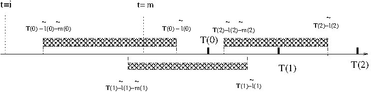
Figure 2: Example of sensibility for first component of the index

To ease the comprehension of formula (16), we explain it for the first index component (commodity one) on figure 2 when the index is only updated tree times at date $T_{0}$, $T_{1}$ and $T_{2}$. At date $i$, the first component of the index corresponding to commodity 1 with delivery at date $m$ has a direct impact on the indexed price at which the gas will be paid for all the dates between $T_{0}$ and $T_{2}$ so the sensibility can be written as the sum of a component for delivery during the first and the second period. $\displaystyle{\sum_{l\in[T(0),T(1)[}}q^{*}(l,Z_{l},Q^{*,j}_{l}(z,Q))$ for example is the optimal consumption on first periode exerciced with the index $I_{T(0)}$ constant on first period and thus the sensibility in equation (16) becomes :

$$\Delta^{1}(i,m,z,Q)=-\frac{a_{1}}{Y_{i}^{1,m}} \left(\frac{1}{\tilde{m}(0)}\mathbb{E}[\displaystyle{\sum_{l\in[T(0),T(1)[}}q^{*}(l,Z_{l},Q^{*,i}_{l}(z,Q))X^{1}_{T(0)}Y_{m}^{1,m}~{}|~{}Z_{i}=z]+\right.$$

$$\left.\frac{1}{\tilde{m}(1)}\mathbb{E}[\displaystyle{\sum_{l\in[T(1),T(2)[}}q^{*}(l,Z_{l},Q^{*,i}_{l}(z,Q))X^{1}_{T(1)}Y_{m}^{1,m}~{}|~{}Z_{i}=z]\right)$$

As for the exchange rate corresponding to component $j$ of the index, introducing

$$D^{j}_{X}(i,m,l,z,Q)=q^{*}(l,Z_{l},Q^{*,i}_{l}(z,Q))Y_{m}^{j},$$

and

$$\bar{D}^{j}_{X}(i,z,Q)=a_{j}\sum_{k,T(k)>i\quad}\sum_{l\in[T(k),T(k+1)[}D^{j}_{X}(i,T(k),l,z,Q)\hat{S^{j}}^{\tilde{l}(k),\tilde{m}(k)}_{T(k)},$$

the sensibility is given by

$$\Delta^{j}_{X}(i,z,Q)=-\mathbb{E}[\bar{D}^{j}_{X}(i,z,Q)~{}|~{}Z_{i}=z]/Y_{i}^{j}$$ (17)

Here for each period $k$ that has not began, we assess the optimal volume exerciced on the period multiplied by the tangent process at $T(k)$ for the exchange rate multiplied by the $a_{j}$ coefficient and the average value of the commodity $j$ used for the index on period $[T(k),T(k+1)[$. The results are obtained by summing on the periods and taking conditional expectation.

3.2 Discretized algorithm

In order to solve equation (8), the methodology in bouchardwarin derived from the Longstaff-Schwartz methodology long2001 can be used as in the case of American options. Using this methodology adapted to Swing option, optimal exercices and corresponding hedging strategies calculated at a date $t$ depend on quantities consumed before this date. So optimal values and hedge have to be calculated on a grid used to discretize the possible volume consumed. Interpolation between Bellman values and hedging strategies is then used during the dynamic programming process.
The volume is discretized on the grid

$$Q_{l}=l\Delta,\quad l=0,\ldots,L=Q_{max}/\Delta$$

where $\Delta$ is the mesh size. Similarly to the case of American option, a Monte Carlo method is used to get some prices simulations $(S_{i}^{j})^{\tilde{j}}$ for $\tilde{j}=1,\ldots,M$ at day $i=0$ to $t_{end}$, for $j=0,...,N$. In the sequel $(.)^{\tilde{j}}$ will stand for the simulation $\tilde{j}$ of random variable $(.)$. The conditional expectation $\mathbb{E}[~{}|~{}Z_{t}]$ has to be calculated in very high dimension but as shown in bernhart , it is possible to approximate the operator $\mathbb{E}[~{}|~{}Z_{i}]$ by the operator $\mathbb{E}[~{}|~{}S^{0}_{i},I_{i}]$ with accuracy leading to regression in dimension 2. In the numerical part of the article a small study on the regressor will be achieved more thoroughly. In the sequel we note $\hat{\mathbb{E}}[~{}|~{}\hat{Z}_{t}]$ an approximation of the conditional expectation operator $\mathbb{E}[~{}|~{}Z_{t}]$ obtained by regression with bouchardwarin methodology where the information contained in the stochastic state vector $Z_{t}$ has been approximated by some information contained in $\hat{Z}_{t}$ vector.

We note $\hat{q}^{*}$ and $\hat{Q}^{*}$ the estimation of the optimal volume $q^{*}$ and optimal volume levels $Q^{*}$ obtained by the Longstaff-Schwartz method. We note $\hat{D}^{0}$, $\hat{D}^{j}$,$\hat{\bar{D}}^{j}$, $\hat{D}^{j}_{X}$, $\hat{\bar{D}}^{j}_{X}$, $j=1,N$ the estimations of the variable $D^{0}$, $D^{j}$,${\bar{D}}^{j}$, $D^{j}_{X}$ and ${\bar{D}}^{j}_{X}$ on Montecarlo simulation for optimal control calculated $\hat{q}^{*}$ .
As explained in warin , knowing $\hat{D}^{0}(i+1,m,(\hat{Z}_{i+1})^{\tilde{j}},Q_{l})$ for $m=i+1,\ldots t_{end}-1$, $l=1,\ldots L$, $\tilde{j}=1,\ldots M$ and using the equality

$$\hat{Q}^{*,i}_{m}((\hat{Z}_{i})^{\tilde{j}},Q)=\hat{Q}^{*,i+1}_{m}((\hat{Z}_{i+1})^{\tilde{j}},Q+\hat{q}^{*}(i,(\hat{Z}_{i})^{\tilde{j}},Q))$$

for $t_{end}>m>i$, the following backward recursion can be used to calculate $\hat{D}^{0}(i,j,Z_{i},Q)$ at day $i$ for all $j\geq i$, for all $Q\in\{Q_{l}/l=0,...,L\}$:

$$\left\{\begin{array}[]{lll}\hat{D}(i,i,(\hat{Z}_{i})^{\tilde{j}},Q)&=&\hat{q}^{*}(i,(\hat{Z}_{i})^{\tilde{j}},Q)(Y_{i}^{0,j})^{\tilde{j}}\\ \hat{D}(i,m,(\hat{Z}_{i})^{\tilde{j}},Q)&=&\hat{D}(i+1,m,(\hat{Z}_{i+1})^{\tilde{j}},Q+\hat{q}^{*}(i,(\hat{Z}_{i})^{\tilde{j}},Q)),m=i+1,t_{end}\end{array}\right.$$ (18)

As for as the current backward recursion on option value, an interpolation on $\hat{D}$ values is necessary to estimate $\hat{D}(i+1,.,.)$ for the stock point $Q+\hat{q}^{*}(i,(\hat{Z}_{i})^{\tilde{j}},Q)$.
The Longstaff-Schwartz estimator of the conditional Delta is then evaluated for $m>k$ by

$$\hat{\Delta}^{0}(i,m,(\hat{Z}_{i})^{\tilde{j}},Q)=\hat{\mathbb{E}}[\hat{D}(i,m,\hat{Z}_{i},Q)~{}|~{}\hat{Z}_{i}=(\hat{Z}_{i})^{\tilde{j}}]/(Y_{i}^{0,m})^{\tilde{j}}.$$ (19)

Similar recursion can be used for $\hat{D}^{j}$ with $j>0$. We first give the $\hat{D}^{j}$ approximation of $D^{j}$ :

$$\hat{D}^{j}(i,m,l,(\hat{Z}_{i})^{\tilde{j}},Q)=q^{*}(l,(\hat{Z}_{l})^{\tilde{j}},Q^{*,i}_{l}((\hat{Z}_{i})^{\tilde{j}},Q))(Y_{m}^{j,m})^{\tilde{j}},i\leq m<l<t_{end}$$ (20)

Introducing $\hat{\bar{D}}^{j}$ the ${\bar{D}}^{j}$ approximation :

$$\hat{\bar{D}}^{j}(i,m,(\hat{Z}_{i})^{\tilde{j}},Q)=a_{j}\sum_{k}\sum_{l\in[T(k),T(k+1)[}D^{j}(i,m,l,(\hat{Z}_{i})^{\tilde{j}},Q)\frac{1_{T(k)-\tilde{l}(k)>m>T(k)-\tilde{l}(k)-\tilde{m}(k)}}{\tilde{m}(k)}$$

we then calculate the $\hat{\bar{D}}^{i}$ values during the recursion easily supposing that $\hat{\bar{D}}^{j}(i+1,j,(\hat{Z}_{j})^{\tilde{j}},Q)$ have been previously calculated with

$$\left\{\begin{array}[]{lll}\hat{\bar{D}}^{j}(i,i,(\hat{Z}_{i})^{\tilde{j}},Q)&=&a_{j}\sum_{k}\sum_{l\in[T(k),T(k+1)[}D^{j}(i,i,l,(\hat{Z}_{i})^{\tilde{j}},Q)X^{j}_{T(k)}\frac{1_{T(k)-\tilde{l}(k)>i>T(k)-\tilde{l}(k)-\tilde{m}(k)}}{\tilde{m}(k)}\\ \hat{\bar{D}}^{j}(i,m,(\hat{Z}_{i})^{\tilde{j}},Q)&=&\hat{\bar{D}}^{j}(i+1,m,(\hat{Z}_{i+1})^{\tilde{j}},Q+\hat{q}^{*}(i,(\hat{Z}_{i})^{\tilde{j}}),Q),i<m\end{array}\right.$$ (21)

Equation (21) allows to calculate the hedge :

$$\hat{\Delta}^{j}(i,m,(\hat{Z}_{i})^{\tilde{j}},Q)=-\mathbb{E}[\hat{\bar{D}}^{j}(i,m,l,\hat{Z}_{i},Q)~{}|~{}\hat{Z}_{i}=(\hat{Z}_{i})^{\tilde{j}}]/(Y_{i}^{j,m})^{\tilde{j}}$$ (22)

As for the exchange rate we introduce $\hat{D}^{j}_{X}$ the $D^{j}_{X}$ approximation :

$$\hat{D}^{j}_{X}(i,m,l,(\hat{Z}_{i})^{\tilde{j}},Q)=q^{*}(l,(\hat{Z}_{l})^{\tilde{j}},Q^{*,i}_{l}((\hat{Z}_{i})^{\tilde{j}},Q))(Y_{m}^{j})^{\tilde{j}},i<m<l$$ (23)

and the $\hat{\bar{D}}^{j}_{X}$ approximation of ${\bar{D}}^{j}_{X}$

$$\hat{\bar{D}}^{j}_{X}(i,(\hat{Z}_{i})^{\tilde{j}},Q)=a_{j}\sum_{k/T(k)>i\quad}\sum_{l\in[T(k),T(k+1)[}\hat{D}^{j}_{X}(i,T(k),l,(\hat{Z}_{i})^{\tilde{j}},Q)(\hat{S^{j}}^{\tilde{l}(k),\tilde{m}(k)}_{T(k)})^{\tilde{j}}$$ (24)

The following recursion adding at each day all the contribution on the sensibility due to the following day can be used during the backward recursion :

$$\left\{\begin{array}[]{lll}\hat{\bar{D}}^{j}_{X}(i,(\hat{Z}_{i})^{\tilde{j}},Q)&=&0,j\geq T(n),\\ \hat{\bar{D}}^{j}_{X}(i,(\hat{Z}_{i})^{\tilde{j}},Q)&=&a_{j}\sum_{k}\delta_{T(k)}(i+1)\sum_{l\in[T(k),T(k+1)[}\hat{D}^{j}_{X}(i,T(k),l,(\hat{Z}_{i})^{\tilde{j}},Q)(\hat{S^{j}}^{\tilde{l}(k),\tilde{m}(k)}_{T(k)})^{\tilde{j}}\\ &&+\hat{\bar{D}}^{j}_{X}(i+1,(\hat{Z}_{i+1})^{\tilde{j}},Q+\hat{q}^{*}(i,(\hat{Z}_{i})^{\tilde{j}},Q)),i<T(n)\end{array}\right.$$ (25)

leading to the Delta approximation

$$\hat{\Delta}^{j}_{X}(i,(\hat{Z}_{i})^{\tilde{j}},Q)=-\mathbb{E}[{\bar{D}}^{j}_{X}(i,\hat{Z}_{i},Q)~{}|~{}\hat{Z}_{i}=(\hat{Z}_{i})^{\tilde{j}}]/(Y_{i}^{j})^{\tilde{j}}$$ (26)

Using equation (18), (19) sensibility with respect to gas is thus calcultated, using equation (21) (22) sensibility with respect to commodity index components calculated and using equation (25) and (26) sensibility to exchange rate calculated.

3.3 Aggregation

Not all product are available on the market. We note ${\cal Q}_{j}^{i}$ the set of future products available at date $i$ for commodity $j$, and for all $p\in{\cal Q}_{i}^{j}$, ${\cal P}_{p}^{j}$ the delivery period associated to product $p$ available for commodity $j$, ${\eta}_{p}^{j}$ the beginning of the delivery period. Supposing that $\forall t>0,\forall p\in{\cal Q}_{i}^{j},\forall\tilde{i}>i$ there exist ${\cal Q}^{j,p}\subset{\cal Q}_{\tilde{i}}^{j}$ such that ${\cal P}_{p}^{j}=\cup_{\tilde{p}\in{\cal Q}^{j,p}}{\cal P}_{\tilde{p}}^{j}$ then it is possible to aggregate an approximated conditional Delta at date $i$ per product with an ad hoc rule so that a dynamic programming approach is still usable. A first way to get the Delta on a delivery period $p$ is to average the Deltas calculated with equations (19) and (22) calculated during recursion on the delivery period. This approach is memory cumbersome as noted in warin . It is far more efficient to calculated the Delta directly on the product $p$ during the backward recursion. warin proposed to use in the continuous framework :

$$\left\{\begin{array}[]{lll}\tilde{D}^{0}(i,p,Z_{i},Q)&=&\mathbb{E}[\sum_{m\in{\cal P}_{p}^{0}}\hat{q}^{*}(m,Z_{m},\hat{Q}^{*,i}_{m}(Z_{i},Q))Y_{m}^{0,m}F^{0}(0,t_{m})~{}|~{}Z_{i}],p\in{\cal Q}_{j}^{0}\\ \tilde{\Delta}^{0}(i,p,Z_{i},Q)&=&{\tilde{D}}^{0}(i,p,Z_{i},Q)/(Y_{i}^{\eta_{p}^{0}}\sum_{m\in{\cal P}_{p}^{0}}F^{0}(0,t_{m}))\end{array}\right.$$

where $\tilde{\Delta}^{0}(i,p,Z_{i},Q)$ represents the power to invest at date $i$ for product $p$ for a gas volume level consumed $Q$ and a stochastic state vector $z$. As shown by warin , the $\tilde{D}^{0}(i,p,z,Q)$ can be calculated during the dynamic programming recursion using :

$$\tilde{D}^{0}(i,p,Z_{i},Q) = \hat{\mathbb{E}}[1_{i+1\in{\cal P}_{p}}\hat{q}^{*}(i+1,Z_{i+1},\hat{Q}^{*,i}_{i+1}(Z_{i},Q))Y_{i+1}^{0,i+1}F^{0}(0,i+1)~{}|~{}Z_{i}]$$

$$+\sum_{\tilde{p}\in{\cal Q}^{0,p}}\hat{\mathbb{E}}[\tilde{D}(i+1,\tilde{p},Z_{i+1},Q+\hat{q}^{*}(i,Z_{i},Q))~{}|~{}Z_{i}=z].$$

The same procedure can be applied to derive a Delta estimation for the index commodity component $j>0$ :

$$\left\{\begin{array}[]{lll}\tilde{D}^{j}(i,p,Z_{i},Q)&=&\mathbb{E}[\sum_{m\in{\cal P}_{p}^{j}}{\bar{D}}^{j}(i,m,Z_{i},Q)F^{j}(0,t_{m})~{}|~{}Z_{i}],p\in{\cal Q}_{i}^{j}\\ \tilde{\Delta}^{j}(i,p,Z_{i},Q)&=&\tilde{D}^{j}(i,p,Z_{i},Q)/(Y_{i}^{\eta_{p}^{j}}\sum_{m\in{\cal P}_{p}^{j}}F^{j}(0,t_{m}))\end{array}\right.$$ (27)

Using equation (15) we get

$$\tilde{D}^{j}(i,p,Z_{i},Q)=\sum_{m\in{\cal P}_{p}^{j}}a_{j}\sum_{k}\sum_{l\in[T(k),T(k+1)[}F^{j}(0,t_{m})\frac{1_{T(k)-\tilde{l}(k)>m>T(k)-\tilde{l}(k)-\tilde{m}(k)}}{\tilde{m}(k)}\mathbb{E}[D^{j}(i,m,l,Z_{i},Q)~{}|~{}Z_{i}]$$

Besides from equation (14)

$$\mathbb{E}[D^{j}(i,m,l,Z_{i},Q)~{}|~{}Z_{i+1}] = \mathbb{E}[q^{*}(l,Z_{l},Q^{*,i}_{l}(Z_{i},Q))Y_{m}^{j,m}~{}|~{}Z_{i+1}],\mbox{for}m>i+1$$

$$= \mathbb{E}[q^{*}(l,Z_{l},Q^{*,i+1}_{l}(Z_{i+1},Q+q^{*}(Z_{i},Q)))Y_{m}^{j,m}~{}|~{}Z_{i+1}]$$

$$= \mathbb{E}[D^{j}(i,m,l,Z_{i+1},Q+q^{*}(Z_{i},Q)~{}|~{}Z_{i+1}]$$

so that

$$\mathbb{E}[D^{j}(i,m,l,Z_{i},Q)~{}|~{}Z_{i}] = \mathbb{E}[D^{j}(i,m,l,Z_{i+1},Q+q^{*}(Z_{i},Q)~{}|~{}Z_{i}]$$

and

$$\tilde{D}^{j}(i,p,Z_{i},Q) = \hat{\mathbb{E}}[1_{i+1\in{\cal P}_{p}^{j}}{\bar{D}}^{j}(i,i+1,l,Z_{i},Q))~{}|~{}Z_{i}]+$$ (28)

$$\sum_{\tilde{p}\in{\cal Q}^{j,p}}\hat{\mathbb{E}}[{\tilde{D}}^{j}(i+1,p,Z_{i+1},Q+q^{*}(Z_{i},Q))~{}|~{}Z_{i}]$$

which can be easily calculated during backward recursion.

4 Numerical results

In first subsection we present the contract used for this study and we give the different numerical parameters used in calculation :

1. the number of basis function used for each dimension for regression used to estimate conditional expectation bouchardwarin ,

2. the number of particules used in an optimization part calculating the optimal value and the conditional hedge store in files,

3. the number of particules used in a simulation part where the dynamic hedge is carried out.

In a second subsection a study on the regression dimension is achieved and in a third subsection we test for the contract the sway of each component on the hedge’s efficiency. At last we test the effect of the hedge frequency on the hedge efficiency.

4.1 Contract description and general parameter

We take the following example derived from a real Swing contract. We suppose that the Swing is contracted for year 2007 and that the day of valorisation is 1th of april 2006. The flexibility is such that each day normalized quantities are such that $q_{max}=0.4$, $Q_{min}=91$,$Q_{max}=146$.

Remark 4

With this kind of parameters the $Q_{max}$ constraint is ineffective.

The arbitrage market taken for $S^{0}$ is the spot gas at Zeebruge hub. The index is composed of two components :

• The first component is described by parameters $(9,0,1)$ such that the average is taken on 9 months ($\tilde{m}$ equivalent to 9 months), with no lag and the index component is changed every month. The first commodity is the brent.

• The second component of the index is described by parameters $(1,0,1)$ meaning that the average is taken during 1 month ($\tilde{m}$ equivalent to 1 month) , no lag ($\tilde{l}=0$) and the index component 2 is changed every month. The second commodity is the month ahead gas on TTF market.

The parameters $a_{i},b_{i}$ have been adapted such that the Swing is at the money (the corresponding swap contract has a zero value) : $a_{0}=2.2$, $a_{1}=0.1757$, $a_{2}=0.2714$, $b_{1}=45.16$, $b_{2}=0$.

The model for each commodity are described by a two factor model ($n=2$) :

• The Brent annual short term volatility is equal to $0.28$, the annual short term mean reverting is equal to $0.1$, and the annual long term volatility is equal to $0.1$, the quotation is in dollar.

• As for the spot/future gas market, the short term annual volatility is equal to $1$, the annual short term mean reverting equal to $80$, while the long term volatility is equal to $0.1$. The quotation is in Euro the domestic market.

• Spread between the euro and dollar interest rate is 0, and the annual volatility between the two currency is $0.11$.

The daily forward curves are generated by Monte Carlo and at each day, depending on the market product available, this curves is averaged on each delivery period associated to each product giving products values that will be used during hedging.

The parameter used for the calculations are the following :

• we use 80000 trajectories in optimization to calculate the Swing value and the hedge,

• when regressing in dimension 1, $6$ basis functions are taken. When regressing in dimension 2, $6\times 4$ basis function are taken, while when regressing in dimension 3, $6\times 4\times 1$ basis functions are taken.

• The global quantities $Q_{l}$ are discretized with a step of $0.4$ and the local quantities with a step $0.1$.

Due to the calculation time and most of all due to the memory needed on computer, the Delta calculations have been parallelized by mpi (http://www.mcs.anl.gov/research/projects/mpi/) on a cluster during optimization and parallelization on scenarios has been achieved in simulation. A single optimization takes roughly 5 hours on 12 cores of a cluster and half an hour in simulation.

4.2 Regression tests

In the section we test three regressors :

• for the first one, we approximate $Z_{t}$ by $S^{0}_{t}$,

• for the second one, we approximate $Z_{t}$ by $(S^{0}_{t},I_{t})$,

• for the last one, we approximate $Z_{t}$ by $(S^{0}_{t},I_{t},\tilde{I}_{t})$ where $\tilde{I}_{t}$ is the partial summation of index that will be used the following month

  $$\tilde{I}_{i}=\sum_{j=1}^{N}a_{j}(\tilde{S^{j}}^{l(k(i)+1),m(k(i)+1)}_{T(k(i)+1),i}-b_{j})x^{j}_{i}$$

  where

  $$\tilde{S^{j}}^{l,m}_{T,i}=\frac{1}{\tilde{m}}\sum_{q=T-\tilde{l}-i}^{\tilde{m}}S^{j}_{T-\tilde{l}-q}$$

  Using the last approximation we take into account the fact that a new index is under construction for the next period.

In the last case, the $I_{t}$ and $\tilde{I}_{t}$ are very correlated and the regression procedure using the Choleski method in the normal equation (see bouchardwarin ) can fail when using many meshes in the last direction. That is the reason why we use only a linear approximation in the last direction.

Remark 5

The regression achieved is depending on the time step. If one regresses on $\hat{Z}_{t}=(S^{0}_{t},I_{t})$ for a current step after $t_{start}$, the regression is only achieved on $S^{0}_{t}$ before $t_{start}$ because $I_{t}$ does not exist. If one regresses on $\hat{Z}_{t}=(S^{0}_{t},I_{t},\tilde{I}_{t})$ for a current step between $t_{start}$ and $t_{end}$, $Z_{t}$ is restricted to $(S^{0}_{t},\tilde{I}_{t})$ before $t_{start}$ and $(S^{0}_{t},I_{t})$ after $T_{\hat{n}}$.

Results obtained in optimization and simulation are given in table 1. Standard deviation of the portfolio with and without hedge is given. In this test, we hedge each component of the index and the exchange rate.

Optimization Simulation Standard deviation value value without hedge with hedge $\hat{Z}_{t}=S^{0}_{t}$ 86.2 86.0 219.3 32.4 $\hat{Z}_{t}=(S^{0}_{t},I_{t})$ 97.7 97.4 204.1 21.3 $\hat{Z}_{t}=(S^{0}_{t},I_{t},\tilde{I}_{t})$ 99.6 99.3 202.9 17.0

Table 1: Tests on regressor

As scheduled, the regression on $\hat{Z}_{t}=S^{0}_{t}$ give bad results in term of value compared to the other regressors and in term of hedge efficiency. The regression on $\hat{Z}_{t}=(S^{0}_{t},I_{t})$ and $\hat{Z}_{t}=(S^{0}_{t},I_{t},\tilde{I}_{t})$ have a far higher value indicating a better optimization than in the first case. The daily hedge is very efficient dividing the standard deviation by $10$ for regressor 2 and even by $14$ for regressor 3.

4.3 Components to hedge

In this subsection we choose to use a daily hedge calculated with regressor 3. On figure 3, we give for the 5 same simulations :

• the hedging position in future october 2006 for Brent (so before the exercice have began) ,

• the hedging position in Brent future for january 2007 for the same simulations,

• the hedging position for january 2007 in gas future,

• the hedging position in foreign currency to hedge the product.

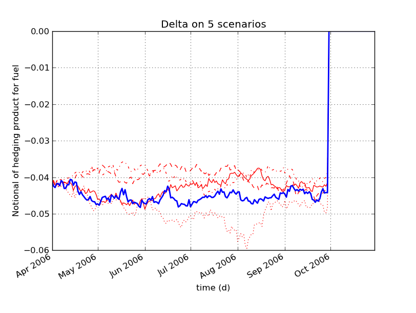
(a) Hedging Brent position october 2006

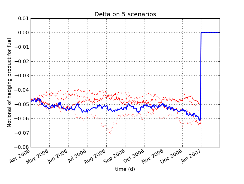
(b) Hedging Brent position january 2007

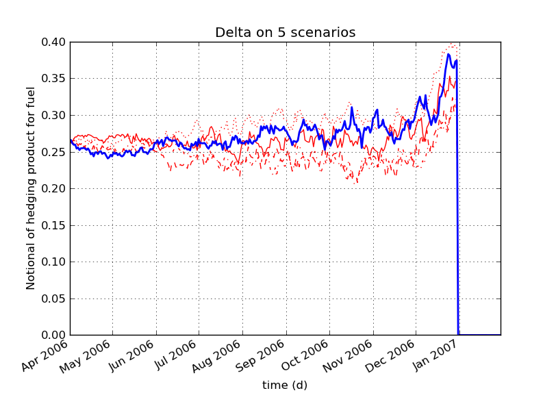
(c) Hedging Gas position january 2007

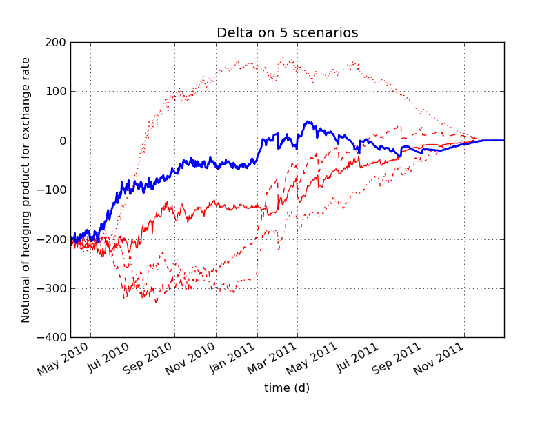
(d) Hedging exchange rate position

Figure 3: Hedging position for different maturities

In table 2 we give the standard deviation obtained in simulation taking different hedge :

• for “Spot gas” we only hedge $S^{0}_{t}$ without taking into account the variation of the index components and exchange rate,

• for “Index components without exchange rate” we only hedge against the variation of the values of the commodities without hedging against gas spot variation and exchange rates variations,

• for “Index components and exchange rate”, we add to the previous hedge an hedge againt the exchange rate variations,

• for “Exchange rate”, we only hedge against the exchange rate variations,

• for “Total hedge” we hedge against all the commodities and exchange rate in the contract.

On this example, it shows that the hedge has to be done against the variations of the index components and that the hedge on gas spot variation is insufficient. It also shows that all the commodities and exchange rate has to be hedged to get an efficient dynamic hedging.

Hedge on Porfolio Standard deviation Spot gas 196.61 Index component without exchange rate 77.20 Index component and exchange rate 74.03 Exchange rate 201.7 Total hedge 17.01

Table 2: Tests on hedge

On figure 4, we give de cash flow distribution obtained while not hedging, while hedging the index components, while hedging against all the product variations.

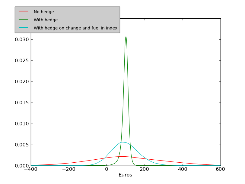
Figure 4: Test on the effectiveness of different hedges

4.4 Frequency of the hedge

It is well know that the hedging error in Black Scholes framework converges to zero at a rate proportional to the square root of hedging frequency zhang ; hayashi . Because the index is evolving quite smoothly, we wonder if we could hedge the derivative less frequently as for the index components : it could help us to decrease the computation time during optimization and would be interesting for practitioners because it would decrease the hedging cost due to illiquidity of the markets. In table 3, we give the standard deviation of the portfolio hedge supposing we hedge all the component but hedging the index with different frequencies. It shows that the effectiveness of the hedge decreases very quickly with the hedge frequency.

Frequency of the index hedge Every day twice a week every week twice a month Standard deviation 17.0 42.9 54.78 57.5

Table 3: Standard deviation of the hedged portfolio with different hedge frequencies for the index components

In table 4, we give the standard deviation of the portfolio hedge supposing we hedge all the component but hedging the index with different frequencies before the first exercice date and balancing the hedging position of the index component every day after the first delivery day.

Frequency of the index hedge before $t_{start}$ every week twice a month every month every quarter Standard deviation 18.6 20.04 20.79 34.89

Table 4: Standard deviation of the hedged portfolio with different hedge frequencies for the index components before the first exercice date and hedging the index components once a day after.

Results in table 4 clearly shows that the hedge frequency can be lowered before the first delivery date without affecting too much the hedging efficiency.

5 Conclusion

We have derived an efficient methodology to hedge dynamically some Swing product on gas market. We have shown that the strategy calculated is very efficient for reducing the standard deviation of the portfolio for a realistic contract. Besides we have shown that on this contract the Swing value is mostly depending on the index component and that an efficient hedge has to deal with all the commodities involved in the index. At last, due to transaction cost it is always interesting to lower the hedge frequency and the last part of the study shows that is could be achieved before the first delivery date without losing too much the hedge efficiency.

References

- (1) O. Bardou, S. Bouthemy, G. Pages : When are Swing options bang-bang and how to use it ? International Journal for Theoretical and Applied Finance, 13(6),867-899 (2010).
- (2) M. Bernhart, P. Tankov, X. Warin: A Finite-Dimensional Approximation for Pricing Moving Average Option. Siam J. Financial Math, 2, 989-1013 (2011)
- (3) R. Bilger : Evaluation of American-Asian Options with the Longstaff-Schwartz Algorithm, M.Sc. thesis, Oxford University, Oxford, UK (2003)
- (4) M. Broadie, M. Cao : Improved lower and upper bound algorithms for pricing American options by simulation. Quant. Finance, 8, 845–861 (2008)
- (5) J.F. Bonnans, Z. Cen, T. Christel : Sensitivity Analysis of Energy Contracts by Stochastic Programming Techniques. Numerical methods in finance, Springer (2012)
- (6) B. Bouchard, X. Warin: Monte-Carlo valorisation of American options: facts and new algorithms to improve existing methods. Numerical methods in finance, Springer (2012)
- (7) L. Clewlow, C. Strickland: Energy derivatives: Pricing and risk management, Lacima (2000)
- (8) M. Dai, P. Li, and J. E. Zhang : A lattice algorithm for pricing moving average barrier options. J. Econom. Dynam. Control, 34, 542–554 (2010)
- (9) E. Gobet: Revisiting the Greeks for European and American options. Proceedings of the ”International Symposium on Stochastic Processes and Mathematical Finance” at Ritsumeikan University, Kusatsu, Japan (2003)
- (10) A. J. Grau : Applications of Least-Squares Regressions to Pricing and Hedging of Financial Derivatives. Ph.D. thesis, University of Munich, Munich, Germany (2008)
- (11) F. Longstaff, E. Schwartz: Valuing American options by simulation: A simple least-squares. Review of Financial Studies, 1(14), 113-147 (2001)
- (12) T. Hayashi, P.A. Mykland: Hedging errors: an asymptotic approach. Mathematical Finance, 15, 309-408 (2005)
- (13) P. Jaillet, R. Ronn, S. Tompaidis: Valuation of commodity-based Swing options. Management science, 50, 909-921 (2004)
- (14) C. H. Kao and Y. D. Lyuu, Pricing of moving-average-type options with applications, J. Futures Market,23, 425-440 (2003)
- (15) F. Longstaff, E. Schwartz: Valuing American options by simulation: A simple least-squares. Review of Financial Studies, 1(14), 113-147 (2001)
- (16) E. S. Schwartz: The Stochastic Behavior of Commodity Prices: Implications for Valuation and Hedging. Journal of Finance, 52, pp. 923- 973 (1997)
- (17) X. Warin : Gas storage hedging. Numerical method in finance, Springer (2012)
- (18) M. Wilhelm, C. Winter: Finite Element valuation of Swing options. Journal of Computational Finance, 11(3),107-132 (2008)
- (19) R. Zhang: Couverture approchée des options Européennes. Phd thesis, Ecole Nationale des Ponts et Chaussées (1999)