Ion-acoustic solitons in warm magnetoplasmas with super-thermal electrons

Abstract

In this work, the phenomenon of formation of localised electrostatic waves (ESW) or soliton is considered in a warm magnetoplasma with the possibility of non-thermal electron distribution. The parameter regime considered here is relevant in case of magnetospheric plasmas. We show that deviation from a usual relaxed Maxwellian distribution of the electron population has a significant bearing in the allowed parameter regime, where these ESWs can be found. We further consider the presence of more than one electron temperature, which is inspired by recent space-based observationskey-2 .

I Introduction

Electrostatic solitary waves (ESW) or solitons are common occurrences in the near-earth plasmas and are routinely observed in the boundary layers and turbulent regions of the magnetosphere key-21 . In recent years, many authors have tried to model these ESWs with the help of different physical models key-2-1 ; key-3-1 ; key-4-1 ; key-5-1 ; key-6-1 ; key-7-1 . Most of the observational and theoretical studies have indicated that these ESWs are basically potential structures (compressive and rarefactive) with density structures (enhancement and compression) and weak double layers key-21 . Solitons or double layers are plasma sheaths (discontinuities) moving in a plasma, which require competing species of charged particles with different masses (inertia) and charges. In an electron-ion plasma, these requirements are fulfilled due to colder ions with their large inertia, which helps in formation of plasma sheaths. So, an electron sheath in a plasma can be effectively modified by equally hot ions key-9-1 .

However, majority of these theoretical analyses do not consider the effect of magnetic field into account. A full-blown analysis of solitary waves where magnetic perturbation is self-consistently considered can be very rigorous key-1 . Several space-borne experiments have observed ESWs moving parallel to the ambient magnetic field in various near-earth plasma environments such as the solar wind, magnetosheath and magnetotail regions, and auroral zone key-2 ; key-3 ; key-4 ; key-5 . These ESWs are, in general, bipolar structures moving in the direction of the background magnetic field key-6 . In the auroral region, these ESWs are reported as negative potential structures travelling upward along the auroral magnetic field lines key-7 ; key-8 . These observations are also supported by those from the Freja satellite data key-9 ; key-10 . Besides, space plasmas, in general, can be largely modeled with Maxwellian velocity distribution. However, advancement of satellite based technologies in recent years, has led to the realization that most of these plasmas, especially the near-earth plasmas, have high energy tails and heat-flux shoulders, which may be attributed to the fact that these plasmas are quite inhomogeneous and semi-collisionless key-11 ; key-12 ; key-13 . Subsequently, it has been established that these plasmas are best modeled by a generalized Lorentzian or kappa distribution (especially the electron distributions) rather than by a pure Maxwellian key-14 ; key-15 . Experimental observations on solar wind plasmas, in recent years, have established that these plasmas have a spectral index key-16 $\sim 2.8$. In the Earth’s magnetosphere, the spectral index is typically observed key-17 in the range $2\leq\kappa\leq 8$. We, in this Chapter, consider these ESWs in the presence of a super thermal electron component.

We, in this work have considered formation of ion-acoustic electrostatic solitary waves in the presence of a background magnetic field. We also consider the electron polulation to be super-thermal, modeled through a Lorentzian or kappa velocity distribution. We further consider the effect of two species of electrons with different temperatures. Presence of multi-temperature electrons in magnetosphere is reported experimentally key-2 . In Section I, we present the plasma model that we have considered for formation of these ESWs in a warm magnetoplasma. In Section II, we consider the solitary wave solutions of the model, where we have incorporated the effect of super-thermal electrons. In Section III, we consider two independent components of super-thermal electrons with two different temperatures. We however have shown that the two-temperature electrons have only marginal effect on the structure and parameter regimes of the ESWs. Finally, we summarise our conclusions in Section IV. The parameter regime considered in this work and the related results can be relevant in explaining large-amplitude ESWs observed in the earth’s magnetosphere.

II Basic model of plasma

Below we write down the basic governing equations for a thermal plasma, which is immersed in an external magnetic field $\bm{B}_{0}$,

$$\frac{\partial n}{\partial t}+\nabla\cdot(n\bm{v}) = 0,$$ (1)

$$\frac{d\bm{v}}{dt} = -\frac{e}{m_{i}}\nabla\phi-\frac{1}{m_{i}}\bm{\nabla}p+(\bm{v}\times\bm{\Omega}),$$ (2)

$$n=n_{e} = F(\phi),$$ (3)

$$p \propto (nm_{i})^{\gamma},$$ (4)

where Eqs.(1) and (2) represent the continuity equation and conservation of momentum for the ions. The function $F(\phi)$ represents equilibrium electron (and ion) density according to the particular velocity distribution function (VDF) i.e. Boltzmanian or kappa distribution. The last equation is the equation of state. In the above equations, $n$ and $n_{e}$ are the ion and electron densities and $\bm{\Omega}=e\bm{B}_{0}/(m_{i}c)$ is the ion gyro-frequency. Other symbols have their usual meanings and quasi-neutrality is assumed all throughout. We assume the external magnetic field to be in the $\hat{\bm{z}}$ direction.

We assume an arbitrary electrostatic perturbation in time and space and define a co-moving coordinate $\eta=l_{x}x+l_{z}z-v_{M}t$, where $l_{x,z}$ are direction cosines and thus defined by the relation $l_{x}^{2}+l_{z}^{2}=1$, and $v_{M}$ is the velocity of the nonlinear wave. Far away from the perturbation we assume everything to be stationary and define the boundary condition as at $\eta\rightarrow\infty,n\rightarrow n_{0},\phi\rightarrow 0,$ and $\bm{v}\rightarrow 0$. Without any loss of generality, we can assume that the physical quantities are constant along $\hat{\bm{y}}$ direction.

II.1 Reduction of equations

We now describe a general procedure for reducing Eqs.(1-4). From the continuity equation, we can write

$$l_{x}v_{x}+l_{z}v_{z}-v_{M}=-v_{M}\frac{n_{0}}{n}.$$ (5)

From the $x,y,$ and $z$ components of the momentum equation, we can write,

$$-v_{M}\frac{n_{0}}{n}v_{x}^{\prime} = -l_{x}[f(n)+g(n)]+v_{y}\Omega,$$ (6)

$$-v_{M}\frac{n_{0}}{n}v_{y}^{\prime} = -v_{x}\Omega,$$ (7)

$$-v_{M}\frac{n_{0}}{n}v_{z}^{\prime} = -l_{z}[f(n)+g(n)],$$ (8)

where the $(^{\prime})$ refers to derivative with respect to the scaled coordinate $\eta$, and $f(n)$ and $g(n)$ functions of $n$,

$$f(n) = \frac{T}{m_{i}(n_{0}^{2}n)^{1/3}}\,n^{\prime},$$ (9)

$$g(n) = \frac{e}{m_{i}}\,\phi^{\prime}.$$ (10)

Here, we have expressed the equilibrium presurre $\gamma p_{0}/n_{0}=T$, with $\gamma$ being the ratio of the specific heats taken as $5/3$. Note that all throughout the calculations, temperature $T$ is expressed in energy units. We now take a derivative of Eqs.(6) and (8) with respect to $\eta$ to get the following relations,

$$-v_{M}\frac{n_{0}}{n}\left(v_{x}^{\prime\prime}-\frac{n^{\prime}}{n}v_{x}^{\prime}\right) = -l_{x}[f^{\prime}(n)+g^{\prime}(n)]+v_{x}\frac{n}{n_{0}}\frac{\Omega^{2}}{v_{M}},$$ (11)

$$-v_{M}\frac{n_{0}}{n}\left(v_{z}^{\prime\prime}-\frac{n^{\prime}}{n}v_{z}^{\prime}\right) = -l_{z}[f^{\prime}(n)+g^{\prime}(n)],$$ (12)

where we have substituted for $v_{y}^{\prime}$ from Eq.(7). By differentiating Eq.(5), successively with respect to $\eta$, we get,

$$l_{x}v_{x}^{\prime}+l_{z}v_{z}^{\prime} = h(n)\equiv v_{M}\frac{n_{0}}{n^{2}}n^{\prime},$$ (13)

$$l_{x}v_{x}^{\prime\prime}+l_{z}v_{z}^{\prime\prime} = p(n)\equiv-2v_{M}\frac{n_{0}}{n^{3}}(n^{\prime})^{2}-v_{M}\frac{n_{0}}{n^{2}}n^{\prime\prime}.$$ (14)

Using Eqs.(11-14), we get,

$$-v_{M}\frac{n_{0}}{n}\left[p(n)-\frac{n^{\prime}}{n}h(n)\right]=-[f^{\prime}(n)+g^{\prime}(n)]+\Omega^{2}\left(\frac{n}{n_{0}}-1\right)-l_{z}v_{z}\frac{n}{n_{0}}\frac{\Omega^{2}}{v_{M}},$$ (15)

where we have used the condition $l_{x}^{2}+l_{z}^{2}=1$ and substituted for $l_{x}v_{x}$ from Eq.(5). Eq.(8) can be integrated to have,

$$v_{z}=\frac{l_{z}}{v_{M}n_{0}}\int n[f(n)+g(n)]\,d\eta+C_{1}\equiv q(n),$$ (16)

where $C_{1}$ is the constant of integration, to be evaluated by imposing the boundary conditions. So, finally, using Eq.(16), from Eq.(15), we arrive at a single nonlinear, second order differential equation for the system as,

$$-v_{M}\frac{n_{0}}{n}\left[p(n)-\frac{n^{\prime}}{n}h(n)\right]=-[f^{\prime}(n)+g^{\prime}(n)]+\Omega^{2}\left(\frac{n}{n_{0}}-1\right)-l_{z}\frac{n}{n_{0}}\frac{\Omega^{2}}{v_{M}}q(n).$$ (17)

We note that the arbitrary functions $f,g,h,p,$ and $q$ can be written entirely as functions of $n$.

III Soliton solutions

In this section, we consider, in general, the electrons to be super thermal governed by Lorentzian or kappa velocity distribution function (VDF). The density of super thermal electrons with a kappa VDF can be written as key-12 ; key-13 ; key-14 ; key-15 ,

$$n=n_{0}\left(1-\frac{2e\phi}{\kappa m_{e}\theta^{2}}\right)^{\nicefrac{{1}}{{2}}-\kappa},$$ (18)

which reduces to the familiar Boltzmann relation in the limit $\kappa\rightarrow\infty$. The temperature is represented by

$$\theta=\left[\left(\frac{2T_{e}}{m_{e}}\right)\frac{\kappa-3/2}{\kappa}\right]^{1/2}.$$ (19)

We note that validity of this particular VDF requires that the spectral index $\kappa\geq 3/2$. The expression for density [Eq.(18)] can be inverted to express the potential $\phi$ as,

$$\phi=\frac{1}{2}\frac{m_{e}}{e}\kappa\theta^{2}\left[1-\left(\frac{n}{n_{0}}\right)^{\frac{2}{1-2\kappa}}\right].$$ (20)

Using the above expression for $\phi$ in the expression for $g(n)$, and carrying out the integration in Eq.(16), we finally write down the explicit nonlinear differential equation in $n$ from Eq.(17) as,

$$\alpha n^{\prime\prime}-\beta(n^{\prime})^{2}+\xi=0,$$ (21)

where

$$\alpha = 15nv_{M}^{2}\left[\sigma n^{8/3}-v_{M}^{2}+n^{2+\frac{2}{1-2\kappa}}\left(\frac{3-2\kappa}{1-2\kappa}\right)\right],$$ (22)

$$\beta = 5v_{M}^{2}\left[\sigma n^{8/3}-9v_{M^{2}}+3n^{2+\frac{2}{1-2\kappa}}\frac{(3-2\kappa)}{(1-2\kappa)^{2}}\right],$$ (23)

$$\xi = 3n^{4}\left[5v_{M}^{2}(1-n)-nl_{z}^{2}(5+3\sigma)+n^{2}l_{z}^{2}\left(3\sigma n^{2/3}+5n^{\frac{2}{1-2\kappa}}\right)\right].$$ (24)

The above equations i.e. Eqs.(21-24) are written in terms of normalized variables. The ion density $n$ is normalized to its equilibrium density $n_{0}$, velocities to the ion-sound velocity $v_{s}=\sqrt{T_{e}/m_{i}}$, potential $\phi$ to $T_{e}/e$, and length to the ratio $v_{s}/\Omega$. The ratio of the ion temperature to the electron temperature is denoted by $\sigma=T/T_{e}$. Note that with this normalizations, the normalized ion velocity $v_{M}$ is the Mach number.

Equation (21) describes the behavior of nonlinear ion-acoustic wave including solutions of solitary waves. However, in order to analytically isolate existence of solitary wave solutions, we need to re-cast Eq.(21) in a form,

$$\frac{1}{2}\left(\frac{dn}{d\eta}\right)^{2}+V(n)=0,$$ (25)

where $V(n)$ is the pseudo or Sagdeev potential key-18 . A potential-well structure of $V(n)$ ensures the existence of solutions of solitary waves. The Eq.(21), however, in its present form with arbitrary $\kappa$ can not be reduced to a form represented by Eq.(25), except in two limiting cases $\kappa\rightarrow\infty$ and $\kappa\rightarrow 3/2$. The first is the well known case of Maxwellian electrons and the second is the extreme limit of super thermal electrons. In what follows, we try to use this two limiting cases.

III.1 Limiting cases

III.1.1 Maxwellian electrons ($\kappa\rightarrow\infty$)

This is a well known case in which Eq.(21) can be reduced to the standard form of Eq.(25), with the quasi potential $V_{\kappa}(n)$ as key-19 ,

$$V_{\infty}(n) = [50v_{M}^{2}(\sigma n^{8/3}+n^{2}-v_{M}^{2})]^{-1}\times\left(n^{6}l_{z}^{2}[5(1-n)+3\sigma(1-n^{5/3})]^{2}\right.$$ (26)

$$-\,5n^{5}v_{M}^{2}[\{10(1-n)(l_{z}^{2}-n)+n\sigma(9+6n^{5/3}-15n^{2/3})$$

$$+\,l_{z}^{2}\sigma(6+9n^{5/3}-15n)\}$$

$$\left.+\,10(l_{z}^{2}-1)n\ln n]+25n^{4}v_{M}^{4}(n-1)^{2})\right).$$

In Fig.1(a), Sagdeev potential for Maxwellian electrons is shown for a certain range of parameters.

Figure 1: (a) Sagdeev potential for Maxwellian electrons and (b) for highly super thermal electrons $(\kappa\sim 3/2)$. The parameters are $v_{M}=0.78,l_{z}=0.7,$ and $\sigma=0.2$. Note the increase in depth and width of the potential in case of super thermal electrons.

III.1.2 Highly super thermal electrons ($\kappa\rightarrow 3/2$)

We now carry out an asymptotic expansion of Eq.(21) in the neighborhood of $\kappa\sim 3/2$. After some simple and straight forward but lengthy algebra, we can reduce Eq.(21) to the following form,

$$\frac{d^{2}}{d\eta^{2}}G(n)=H(n),$$ (27)

where,

$$G(n) = v_{M}^{2}\frac{1}{n^{2}}+(3-2\kappa)\frac{1}{n}+3\sigma n^{2/3},$$ (28)

$$H(n) = 2(n-1)+\left(\frac{l_{z}}{v_{M}}\right)^{2}\left[(3-2\kappa)n\,\ln n-\frac{6}{5}n(n^{5/3}-1)\right].$$ (29)

Multiplying both sides of Eq.(27) by $dG(n)/d\eta$ and integrating, we to get,

$$\frac{1}{2}\left(\frac{d}{d\eta}G(n)\right)^{2}=\int H(n)\,\frac{d}{d\eta}G(n)\,d\eta+C_{2},$$ (30)

from which, we can finally write the standard form for the quasi potential equation in the form of Eq.(25) with the quasi or Sagdeev potential as,

$$V_{\nicefrac{{3}}{{2}}}(n) = [50v_{M}^{2}\{2v_{M}^{2}+n(3-2\kappa-2n^{5/3}\sigma)\}]^{-1}\times\left(n^{6}l_{z}^{2}[6\sigma(n^{5/3}-1)\right.$$ (31)

$$-\,5\ln n(3-2\kappa)]^{2}+100n^{4}v_{M}^{4}(n-1)^{2}$$

$$+\,n^{4}v_{M}^{2}[100n(3-2\kappa)\{(l_{z}^{2}-1)(n-1)-(l_{z}^{2}-n)\ln n\}$$

$$\left.-\,60n\sigma\{3n+n^{5/3}(2n-5)+l_{z}^{2}(2-5n+3n^{5/3})\}]\right).$$

The constant of integration $C_{2}$ is evaluated by demanding the boundary condition $V(n)|_{n=1}=0$. The Sagdeev potential for this limiting case is shown in Fig.1(b). In Fig.2(a), we have shown the domain of existence of a soliton in the $(v_{M}-l_{z}-\sigma)$ parameter space for both these limiting cases. A soliton, if any, can exist only left of the surfaces (please see the captions for details). The projection of the domains in the $(v_{M}-l_{z})$ space is shown in Fig.2(b). The left side of the regions are limited by $\sigma\rightarrow 0$. In the overlapping region, solitons in both extreme cases can form.

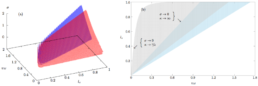
Figure 2: (a) Domains of existence of solitons in the two limiting cases in the $(v_{M},l_{z},\sigma)$ parameter space. Solitons exist only left sides of the surfaces. The surface on the front (red) is for $\kappa\sim 3/2$ and the other (blue) is for $\kappa\rightarrow\infty$. (b) Projection of the surfaces showing the regions of existence of solitons in the $(v_{M},l_{z})$ space. The right side boundaries of the regions are for higher $\sigma$.

III.1.3 Limiting Mach numbers

The limiting Mach numbers can be found out by imposing the condition that $V(n)$ must have a local maximum at $n=1$, which translates to the conditions

$$l_{z}\sqrt{1+\sigma}<v_{M}<\sqrt{1+\sigma},$$ (32)

for Maxwellian electrons and

$$l_{z}\sqrt{\kappa-3/2+\sigma}<v_{M}\sqrt{\kappa-3/2+\sigma}.$$ (33)

for highly super thermal electrons ($\kappa\sim 3/2$). The latter condition reduces to $l_{z}\sqrt{\sigma}<v_{M}<\sqrt{\sigma}$ for $\kappa\rightarrow 3/2$ . So, with highly Lorentzian electrons, solitons can form even with lower values of Mach numbers. In Fig.3, we have shown the dependence of soliton amplitude $A$ and width $\Delta$, respectively, with the Mach number for both these cases. Note that the amplitude $A$ is determined by first zero of the Sagdeev potential away from $n=1$ and the soliton width $\Delta=A/\sqrt{d}$, where $d$ is the maximum depth of the Sagdeev potential determined by the condition $dV(n)/dn|_{n\neq 1}=0$. As can be seen from Fig.3, in case of highly super-thermal electrons, the soliton can be very steep (smaller width) and can reach high amplitude in comparison with thermal electrons.

Note that the range of the valid Mach number is exclusively dictated by the direction of propagation of the soliton with the higher limit parallel to the magnetic field ($l_{z}\rightarrow 1$).

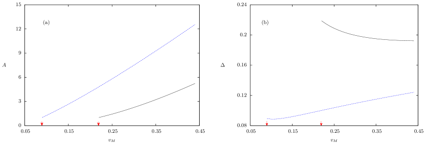
Figure 3: (a) Dependences of soliton amplitude $A$ on Mach number. (b) Dependences of soliton width $\Delta$ on Mach number. The arrows show the position of lower limits of the respective Mach numbers. The blue (dashed) curves are for $\kappa\sim 3/2$ and the solid (black) curves are for $\kappa\rightarrow\infty$ (Maxwellian electrons). The parameters are same as in Fig.1.

III.2 Arbitrary $\kappa$ — numerical solution

As mentioned earlier, Eq.(21) can not be reduced to standard form for arbitrary $\kappa$, which can analytically demonstrate the existence of a suitable quasi potential and thus solitary wave solutions, which however, does not rule out existence of soliton-like solutions for arbitrary $\kappa$. In order to solve the second order, nonlinear differential equation, Eq.(21) numerically for solitary wave solutions, we use the shooting method, imposing the boundary conditions $n(\eta)|_{\eta\rightarrow\pm M}=1$ and start with an initial condition $n^{\prime}(\eta)|_{\eta=0}=0$, where $M$ is a large number. In practice, we need to solve only one half on the $\eta$-axis in the range $\eta\in[0,+M]$ as the the solutions $n(\eta)$ are always symmetric in the range $[-M,+M]$, which can be easily seen from the invariance of Eq.(21) for $\eta\rightarrow-\eta$. In Fig.4(a), we have shown the evolution of the soliton as obtained from numerical solution of Eq.(21) for arbitrary $\kappa$. The corresponding bi-polar electric field representing the solitary density structure is shown in Fig.4(b). Note that the corresponding electric field for a density soliton can be found from the relation,

$$E(\eta)=-\frac{1}{n}\,\frac{dn}{d\eta}.$$ (34)

We note that in the auroral region, the ion to electron temperature ratio $\sigma\sim 0.25$ and the ion gyro frequency $(\Omega/2\pi)\sim 100\,{\rm Hz}$ key-22 . Consider now various bi-polar electrostatic structures observed in different regions viz. auroral region of the ionosphere and earth’s magnetosphere. These structures show peak-to-peak variation of electric field ranging from few hundreds of micro volts per meter to milli volts per meter within an interval of micro seconds to milli seconds. Usually the amplitudes of pulses in the auroral region are larger (milli volts per meter) having a larger duration of the order of milli seconds key-7 . Those observed in the magnetosheath region are of much smaller amplitudes (micro volts per meter) with a very short duration (micro seconds) key-21 . Note that the bi-polar structures represented in Fig.4(b) are in the rest frame of the solitons, which can be transformed to the duration of the pulses in the rest frame of the detector (on board the satellite). In Fig.5, we show various bi-polar electrostatic structures for these parameters in real-time units. In all panels of Fig.5, the pulse is of shorter duration and larger height for highly Lorentzian electrons than Maxwellian electrons. The peak-to-peak electric field variation due to Lorentzian electrons in panel (d) is $\sim 250\,{\rm mV}/{\rm m}$ with a duration $\sim 20\,{\rm ms}$, which is typical in these regions key-7 ; key-22 . For the same parameters, the peak-to-peak variation is much smaller $\sim 90\,{\rm mV}/{\rm m}$ with a longer duration $\sim 40\,{\rm ms}$ for Maxwellian electrons. The pulses due to Maxwellian electrons are comparable to Lorentzian electrons in both pulse height and width only when the pulses become very large, which are however, not observed in these regions of space plasma. So, we conclude that the deviation of electron temperature from thermal behavior is an essential factor, which needs to be taken into account in order to explain the relatively small-amplitude and steep (smaller width) bi-polar electrostatic structures in the auroral regions.

We further note that the effect due to super-thermal electrons is more pronounced when $l_{z}\sim 1$ or $\theta\sim 0^{\circ}$, where $\theta$ defines the angle between the ambient magnetic field and the direction of propation of the soliton. This is consistent with observvation of these solitons in magnetospheric plasmaskey-2 ; key-3 ; key-4 ; key-5 .

IV Two-temperature electrons : small amplitude solitons

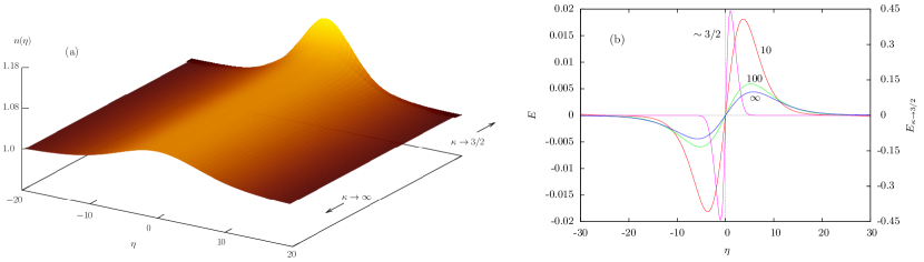
Figure 4: (a) Evolution of soliton as $\kappa$ approaches $3/2$ from a large value. (b) The bi-polar electric field corresponding to (a). Use the right hand side axis for the case when $\kappa\sim 3/2$, which is very large compared to others.

In this section, we consider the physical scenario with two-temperature electrons, which is motivated by the experimental observations such as those by the Cluster spacecrafts key-2 . We consider two species of electrons — hot and cold one. We still assume that both species of electrons are Lorentzian, which gives us freedom to investigate the situation both for thermal and super-thermal cases. All mathematical analyses remaining same, differing only in the expression denoting the combined density of the electrons [see Eq.(18)],

$$n_{e}=n_{c}+n_{h}=n_{c0}\left(1-\frac{2e\phi}{\kappa m_{e}\theta_{c}^{2}}\right)^{\nicefrac{{1}}{{2}}-\kappa}+n_{h0}\left(1-\frac{2e\phi}{\kappa m_{e}\theta_{h}^{2}}\right)^{\nicefrac{{1}}{{2}}-\kappa},$$ (35)

and the quasi-neutrality condition [see Eq.(3)],

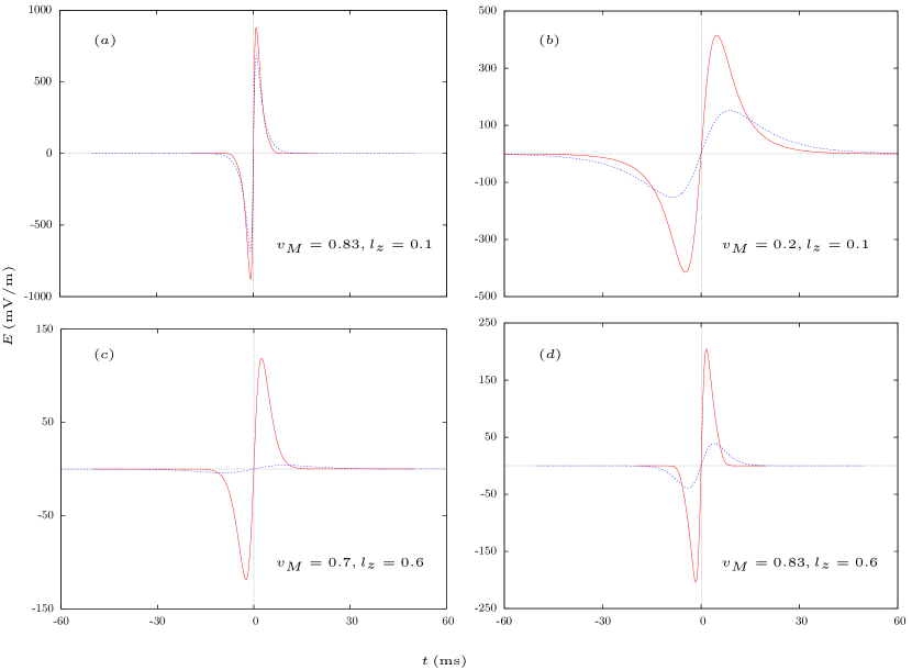
Figure 5: Bi-polar electrostatic pulse in real-time units. The solid (red) curves are for highly Lorentzian electrons ($\kappa\sim 3/2$) and the dashed (blue) curves are for Maxwellian electrons.

$$n=n_{c}+n_{h},$$ (36)

where the subscripts ‘$c$’ and ‘$h$’ refer to the cold and hot electrons with $\theta_{c,h}$ respectively being functions of $T_{c,h}$, the temperatures of cold and hot electrons. The primary drawback in this formalism that we can not find an equivalent Sagdeev potential for solitons of arbitrary amplitudes as Eq.(35) can not be inverted to find a unique analytical expression for the potential $\phi$ in terms of the densities. In what follows, we shall expand Eq.(35) around $\phi=0$, assuming the analysis for only small-amplitude solitons, so that we can find out the Sagdeev potential which, however, will be valid only in the limit of small amplitude.

A Taylor expansion of Eq.(35) around $\phi=0$, to the zeroth order enables us to write the plasma potential (un-normalized) as,

$$\phi\simeq\frac{T_{c}T_{h}}{e}\left(\frac{n-n_{c0}-n_{h0}}{n_{c0}T_{h}+n_{h0}T_{c}}\right)\left(\frac{2\kappa-3}{2\kappa-1}\right).$$ (37)

As before, we normalize the variables and write the normalized electron densities as $\nu_{c,h}=n_{c0,h0}/n_{0}$ with the condition $v_{c}+v_{h}=1$. The temperature ratio of the cold and hot electrons is $\beta=T_{c}/T_{h}$ and $\sigma=T/T_{h}$. Proceeding as before, we can reduce the equations to the form given by Eq.(25) and write the Sagdeev potential (for small amplitude, $n\rightarrow 1$) as

$$V_{n\rightarrow 1}\simeq\frac{n^{4}[100f_{1}^{2}v_{M}^{4}\delta n^{2}+\delta n_{1}^{2}-20nf_{1}v_{M}^{2}\{5f_{2}(n+l_{z}^{2})\delta n^{2}+\delta n_{2}\}]}{200v_{M}^{2}(f_{1}\sigma n^{8/3}-f_{1}v_{M}^{2}+f_{2}n^{3})},$$ (38)

where $\delta n=n-1$ and other quantities are given by,

$$\left.\begin{array}[]{rcl}f_{1}&=&(2\kappa-1)\,\{1-\nu_{h}(1-\beta)\},\\ \\ f_{2}&=&(2\kappa-3)\beta,\\ \\ \delta n_{1}&=&5f_{2}l_{z}(n^{2}-1)+6f_{1}l_{z}\sigma(n^{5/3}-1),\\ \\ \delta n_{2}&=&3f_{1}\sigma[3n+n^{5/3}(2n-5)+l_{z}^{2}(3n^{5/3}-5n+2).\end{array}\right\}$$ (39)

The quantities $\delta n,\delta n_{1,2}\rightarrow 0$ as $n\rightarrow 1$ and it is easy to see that the function $V_{n\rightarrow 1}$ satisfies all the requirements of Sagdeev potential. However, its interpretation is valid only in the limit $n\rightarrow 1$.

To complete the analysis, we now take the small amplitude limit of the $V_{n\rightarrow 1}$ in Eq.(25) by expanding around $n=1$. The resultant equation, to the third order, is,

$$\frac{1}{2}\left(\frac{d}{d\eta}\delta n\right)^{2}+\chi_{1}\,\delta n^{2}+\chi_{2}\,\delta n^{3}=0,$$ (40)

which we recognize as the Korteweg de-Vries (K-dV) equation in the transformed space-time co-ordinate $\eta$, describing soliton solutions. The factors $\chi_{1}$ and $\chi_{2}$ are given by

$$\chi_{1} = \frac{f_{1}v_{M}^{2}-f_{3}l_{z}^{2}}{2v_{M}^{2}f_{4}},$$ (41)

$$\chi_{2} = \frac{1}{18v_{M}^{2}f_{4}^{2}}\left[3f_{1}f_{2}l_{z}^{2}(7\sigma-15v_{M}^{2})+9l_{z}^{2}f_{2}^{2}\right.$$ (42)

$$\left.+\,4f_{1}^{2}\{9v_{M}^{4}+3l_{z}^{2}\sigma^{2}-v_{M}^{2}\sigma(1+11l_{z}^{2})\}\right]$$

and

$$\left.\begin{array}[]{rcl}f_{3}&=&f_{2}+f_{1}\sigma,\\ \\ f_{4}&=&f_{1}v_{M}^{2}-f_{3}.\end{array}\right\}$$ (43)

In the above equations, we note that the factors $f_{1,2,3}\geq 0$. The amplitude $A$ and width $\Delta$ of this K-dV soliton is given by,

$$A = -\frac{\chi_{1}}{\chi_{2}},$$ (44)

$$\Delta = \sqrt{-\frac{2}{\chi_{1}}},$$ (45)

so that for existence of a soliton, $\chi_{1}<0$, which translates to the condition,

$$l_{z}\sqrt{f_{\kappa}+\sigma}<v_{M}<\sqrt{f_{\kappa}+\sigma},$$ (46)

where the factor

$$f_{\kappa}=\frac{f_{3}}{f_{1}}=\frac{\beta(2\kappa-3)}{(2\kappa-1)\,\{1-\nu_{h}(1-\beta)\}},$$ (47)

represents the effect of two-temperature electrons. Under various limiting cases, we can reduce this condition to simple forms,

$$l_{z}\sqrt{\frac{\beta}{1-\nu_{h}(1-\beta)}+\sigma} < v_{M}<\sqrt{\frac{\beta}{1-\nu_{h}(1-\beta)}+\sigma},\qquad\kappa\rightarrow\infty$$ (48)

$$l_{z}\sqrt{\frac{\beta(\kappa-3/2)}{1-\nu_{h}(1-\beta)}+\sigma} < v_{M}<\sqrt{\frac{\beta(\kappa-3/2)}{1-\nu_{h}(1-\beta)}+\sigma},\qquad\kappa\rightarrow 3/2$$ (49)

which further reduce to (32) and (33) if we consider only single temperature for electrons ($\nu_{h}\rightarrow 1$). As the factor $f_{\kappa}$ lies between zero and unity, the effect of two different temperatures is not very significant expect when $\sigma$ is small. We however note that the parameters $\beta$ and $\nu_{h}$ related to two different temperatures can dictate the exact parameter regime, where solitons may exist.

V Conclusions

In this paper, we have discussed the physical situation where electrostatic solitary structures can form in a warm plasma immersed in a constant background magnetic field and in the presence of a non-thermal electron fluid. The results are viewed in reference to the bi-polar ESWs, typically observed in the auroral regions. We have shown that in presence of a super-thermal electron population, large amplitude solitary structure can form in the parallel direction, which otherwise is not possible for Maxwellian electrons. We have also emphasised that with a super-thermal electron fluid, solitons can form for lower Mach numbers. We have presented our results in the real-time units of the bi-polar ESWs, which are basically manifestations of solitary waves, and our results are in good agreement to the available experimental data in the auroral region.

We have further considered the presence of two components of electron populations, both of which can be super-thermal, in view of the observations by the certain space-borne experiments viz. Cluster spacecrafts key-21 . However we find only marginal modifications to the ESWs by including the two-temperature electrons, and conclude that they may have only minor role in dictating the exact parameter details of the ESWs.

References

- (1) J. S. Pickett et. al., Adv. Space Res. 41, 1666 (2008).
- (2) B. T. Tsurutani, J. K. Arballo, G. S. Lakhina, C. M. Ho, B. Buti, J. S. Pickett, and D. A. Gurnett, Geophys. Res. Lett. 25, 4117 (1998).
- (3) G. S. Lakhina, B. T. Tsurutani, H. Kojima, and H. Matsumoto, J. Geophys. Res. 105, 27791 (2000).
- (4) J. R. Franz, P. M. Kintner, J. S. Pickett, and L.-J. Chen, J. Geophys. Res. 110 A09212 (2005).
- (5) L.-J. Chen, J. S. Pickett, P. Kintner, J. Franz, and D. Gurnett, J. Geophys. Res. 110 A09211 (2005).
- (6) J. D. Williams, L.-J. Chen, W. S. Kurth, D. A. Gurnett, M. K. Dougherty, and A. M. Rymer, Geophys. Res. Lett. 32 L17103 (2005).
- (7) J. D. Williams, L.-J. Chen, W. S. Kurth, D. A. Gurnett, and M. K. Dougherty, Geophys. Res. Lett. 33, L06103 (2006).
- (8) M. P. Bora, B. Choudhury, and G. C. Das, Astrophys. Sp. Sc. (2012).
- (9) P. Meuris and F. Verheest, Phys. Lett. A 219, 2992 (1996).
- (10) J. S. Pickett et. al., Ann. Geophys. 22, 2515 (2004).
- (11) G. T. Marklund et. al., Nonlin. Processes Geophys. 11, 709 (2004).
- (12) M. Temerin, K. Cerny, W. Lotko, and F. S. Mozer, Phys. Rev. Lett. 48, 1175 (1982).
- (13) R. Boström et. al., Phys. Rev. Lett. 61, 82 (1988).
- (14) F. S. Mozer et. al., Phys. Rev. Lett. 79, 1281 (1997).
- (15) S. Bounds et. al., J. Geophys. Res. 104, 28709 (1999).
- (16) J. Dombeck et. al., J. Geophys. Res. 106, 19013 (2001).
- (17) P. Dovner, A. Eriksson, R. Boström, and B. Holback, Geophys. Res. Lett. 21, 1827, (1994).
- (18) Y. Chen, Z.-Y. Li, W. Liu, and Z.-D. Shi, Phys. Plasmas 7, 371 (2001).
- (19) E. Marsch et. al., J. Geophys. Res. 87 (A1), 52 (1982).
- (20) C.-Y. Ma and D. Summers, Geophys. Res. Lett. 25, 4099 (1998).
- (21) D. Summers, S. Xue, and R. M. Thorne, Phys. Plasmas 1, 6 (1994).
- (22) D. Summers and R. M. Thorne, Phys. Fluids B 3, 1835 (1991).
- (23) D. Summers and R. M. Thorne, J. Geophys. Res. 97 (A11), 16827 (1992).
- (24) M. N. S. Qureshi et al., Proc. Tenth Int. Solar Wind Conf. p 489 (2003).
- (25) O. A. Pokhotelov, O. G. Onishchenko , M. A. Balikhin, L. Stenflo, and P. K.Shukla, J. Plasma Phys. 73, 981 (2007).
- (26) R. Z. Sagdeev, Rev. Plasma Phys. 4, 23 (1966).
- (27) M. K. Kalita and S. Bujarbarua, J. Phys. A 16, 439 (1983).
- (28) J. Shi et. al., Ann. Geophys. 26, 1431 (2008).