Support Recovery with Sparsely Sampled
Free Random Matrices

Abstract

Consider a Bernoulli-Gaussian complex $n$-vector whose components are $V_{i}=X_{i}B_{i}$, with $X_{i}\sim{\cal C}{\cal N}(0,{\cal P}_{x})$ and binary $B_{i}$ mutually independent and iid across $i$. This random $q$-sparse vector is multiplied by a square random matrix ${\bf U}$, and a randomly chosen subset, of average size $np$, $p\in[0,1]$, of the resulting vector components is then observed in additive Gaussian noise. We extend the scope of conventional noisy compressive sampling models where ${\bf U}$ is typically a matrix with iid components, to allow ${\bf U}$ satisfying a certain freeness condition. This class of matrices encompasses Haar matrices and other unitarily invariant matrices. We use the replica method and the decoupling principle of Guo and Verdú, as well as a number of information theoretic bounds, to study the input-output mutual information and the support recovery error rate in the limit of $n\to\infty$. We also extend the scope of the large deviation approach of Rangan, Fletcher and Goyal and characterize the performance of a class of estimators encompassing thresholded linear MMSE and $\ell_{1}$ relaxation.

I Introduction

I-A Model Setup

Consider the $n$-dimensional complex-valued observation model:

$${\bf y} = {\bf A}{\bf U}{\bf X}{\bf b}+{\bf z}$$ (1)

$$= {\bf A}{\bf U}{\bf v}+{\bf z}$$ (2)

where:

• ${\bf X}={\hbox{diag}}({\bf x})$, and ${\bf x}$ is an iid complex Gaussian $n$-vector with components $x_{i}\sim{\cal C}{\cal N}(0,{\cal P}_{x})$;

• ${\bf b}$ is an iid $n$-vector with components $b_{i}\sim$ Bernoulli-$q$, i.e., $\mathbb{P}[b_{i}=1]=q=1-\mathbb{P}[b_{i}=0]$;

• ${\bf v}={\bf X}{\bf b}$ is a Bernoulli-Gaussian vector, with components $v_{i}=x_{i}b_{i}$;

• ${\bf A}$ is an $n\times n$ diagonal matrix with iid diagonal elements $[{\bf A}]_{i,i}\sim$ Bernoulli-$p$, i.e., $\mathbb{P}[[{\bf A}]_{i,i}=1]=p=1-\mathbb{P}[[{\bf A}]_{i,i}=0]$;

• ${\bf U}$ is an $n\times n$ random matrix such that

  $${\bf R}={\bf U}^{\dagger}{\bf A}^{\dagger}{\bf A}{\bf U}$$ (3)

  is free from any deterministic Hermitian matrix (see [38] and references therein).

• ${\bf z}$ is an iid complex Gaussian $n$-vector with components $z_{i}\sim{\cal C}{\cal N}(0,1)$;

• ${\bf A}$, ${\bf U}$, ${\bf X}$, ${\bf b}$ and ${\bf z}$ are mutually independent.

• The signal-to-noise ratio (SNR) of the observation model (1) is defined as

  $${\sf SNR}=\frac{\mbox{\bb E}[\|{\bf v}\|^{2}]}{\mbox{\bb E}[\|{\bf z}\|^{2}]}=q{\cal P}_{x}.$$ (4)

The non-zero elements of ${\bf b}$ define the support of the Bernoulli-Gaussian vector ${\bf v}$, whose “sparsity” (average fraction of non-zero elements) equal to $q$. The non-zero diagonal elements of ${\bf A}$ define the components of the product ${\bf U}{\bf v}$ for which a noisy measurement is acquired. In the literature, the number of non-zero diagonal elements of ${\bf A}$ is commonly referred to as the number of measurements. The “sampling rate” (average fraction of observed components) of the observation model (1) is equal to $p$. The sensing matrix ${\bf A}{\bf U}$ is known to the signal processor, the goal of which is to detect the support of ${\bf v}$, i.e., to find the position of the non-zero components of ${\bf b}$.

In this paper we are interested in the optimal performance of the recovery of the sparse signal support. Denoting the recovered support by $\widehat{{\bf b}}=(\widehat{b}_{1},\ldots,\widehat{b}_{n})^{\sf T}$, with $\widehat{b}_{i}\in\{0,1\}$, the objective is to minimize the support recovery error rate:

$$D^{(n)}(p,q,{\cal P}_{x})=\frac{1}{n}\sum_{i=1}^{n}\mbox{\bb P}[b_{i}\neq\widehat{b}_{i}],$$ (5)

where the expectation is with respect to ${\bf A}$, ${\bf U}$, ${\bf X}$, ${\bf b}$, and ${\bf z}$. In particular, this works focuses on the large $n$ regime

$$D(p,q,{\cal P}_{x})=\lim_{n\rightarrow\infty}D^{(n)}(p,q,{\cal P}_{x})$$ (6)

under the optimal Maximum A Posteriori Symbol-By-Symbol (MAP-SBS) estimator, as well as under some popular suboptimal but practically implementable estimation algorithms.

I-B Existing results

Recovery of the sparsity pattern with vanishing error probability is studied in a number of recent works such as [1, 2, 14, 27, 39, 40]. When $k=\sum_{i=1}^{n}b_{i}$, the number of nonzero coefficients in ${\bf v}$, is known beforehand and their magnitude is bounded away from zero, exact support recovery requires that the number of measurements grow as $k\log n$ [14, 40]. If the support recovery error rate is allowed to be non-vanishing, fewer measurements are necessary. Under various assumptions, [1, 2, 29] show that a number of measurements growing proportionally to $k\log\frac{n}{k}$ suffices. A more refined analysis is given by Reeves and Gastpar in [29, 30, 31, 32], assuming that the entries of the measurement matrix are iid but without requiring the signal vector ${\bf x}$ to be Gaussian. They find tight bounds on the behavior of the proportionality constant as a function of SNR and the target support recovery error rate. In particular, [31] upper bounds the required difference $p-q$ when using an ML estimator of the support. The comparison given in [31, 32] of computationally efficient algorithms such as linear MMSE estimation and Approximate Message Passing (AMP) to information theoretic bounds reveals that the suboptimality of those algorithms increases with SNR. In contrast to (5), [32] considers a distortion measure which is the maximum of the false-alarm and missed detection probability.

The recent work [3] gives results for iid Gaussian measurement matrices, based on the analysis of a message passing algorithm rather than the replica method. A full rigorization of the decoupling principle introduced in [18] has been recently announced in [8] for compressive sensing applications with iid measurement matrices. Another rigorous justification of previous replica-based results is given in [43] which shows that iid Gaussian sensing matrices incur no penalty on the phase transition threshold with respect to an optimal nonlinear encoding.

It is of considerable interest to explore the degree of improvement afforded by dropping the assumption that the measurement matrix has iid coefficients. Randomly sampled Discrete Fourier Transform (DFT) matrices (where rows/columns are deleted independently) e.g. [37] are one example of such matrices. The model considered in Section I-A allows a relevant generalization of the iid measurement model, which is analytically tractable.

I-C Organization

Section II gives expressions for the input-output mutual information rate, and shows how to use it in order to lower bound the support recovery error rate. We write the mutual information of interest as the difference of two mutual information rates. The first term is obtained using the heuristic replica-method, previously applied in various problems involving iid matrices, e.g. [18, 35, 28, 15]. The second term is given rigorously, using free probability and large random matrix theory.

Upper and lower bounds on the input-output mutual information corroborating the replica analysis are developed in Section III. We also give a converse result that shows that (6) is bounded away for zero if $p\leq q$. Numerical examples illustrate the tightness of the bounds.

Section IV extends the decoupling principle [18] to the model in (1) and provides the analysis of three support estimators: optimal MAP-SBS, thresholded linear MMSE and $\ell_{1}$ relaxation (Lasso).

Proofs and other technical details are given in the Appendices.

II Mutual information rate

In this section we are concerned with the mutual information rate

$${\cal I} \stackrel{{\scriptstyle\Delta}}{{=}} \lim_{n\to\infty}\frac{1}{n}I({\bf b};{\bf y}|{\bf A},{\bf U})={\cal I}_{1}-{\cal I}_{2}$$ (7)

where

$${\cal I}_{1} \stackrel{{\scriptstyle\Delta}}{{=}} \lim_{n\to\infty}\frac{1}{n}I({\bf v};{\bf y}|{\bf A},{\bf U})$$ (8)

$${\cal I}_{2} \stackrel{{\scriptstyle\Delta}}{{=}} \lim_{n\to\infty}\frac{1}{n}I({\bf x};{\bf y}|{\bf A},{\bf U},{\bf b}).$$ (9)

and the right-most equality in (7) follows from

$$I({\bf b};{\bf y}|{\bf A},{\bf U}) = I({\bf x},{\bf b};{\bf y}|{\bf A},{\bf U})-I({\bf x};{\bf y}|{\bf A},{\bf U},{\bf b})$$ (10)

$$= I({\bf X}{\bf b};{\bf y}|{\bf A},{\bf U})-I({\bf x};{\bf y}|{\bf A},{\bf U},{\bf b})$$ (11)

II-A Error rate lower bound via mutual information

We can bound the minimal support recovery error rate $D(p,q,{\cal P}_{x})$ defined in (5) in terms of ${\cal I}$ using the following simple result.

Theorem 1

Given a joint distribution $P_{XY}$ on $\mathcal{X}\times\mathcal{Y}$, a reconstruction alphabet $\widehat{\mathcal{X}}$ and a distortion measure $\mathsf{d}\colon\mathcal{X}\times\widehat{\mathcal{X}}\mapsto[0,\infty)$, let

$$R(d) \stackrel{{\scriptstyle\Delta}}{{=}} \inf_{P_{\widehat{X}|X}\colon\mathbb{E}[\mathsf{d}(X,\widehat{X})]\leq d}I(X;\widehat{X})$$ (12)

Then

$$R(\inf\mathbb{E}[\mathsf{d}(X,\widehat{X})])\leq I(X;Y)$$ (13)

where the infimum is over all conditional probability assignments $P_{\widehat{X}|Y}$ such that $P_{XY\widehat{X}}=P_{X}P_{Y|X}P_{\widehat{X}|Y}$.

Proof:

See Appendix A ∎

Since $R(d)$ is a monotonically decreasing function, (13) gives an information theoretic lower bound on the non-information-theoretic quantity $\inf\mathbb{E}[\mathsf{d}(X,\widehat{X})]$. In our case, using the rate-distortion function of a Bernoulli-$q$ source with Hamming distortion, given by $R(d)=\max\{h(q)-h(d),0\}$, Theorem 1 results in

$$D(p,q,{\cal P}_{x})\geq h^{-1}(h(q)-\mathcal{I})$$ (14)

where $h(x)=x\log\frac{1}{x}+(1-x)\log\frac{1}{1-x},\;x\in[0,1]$ denotes the binary entropy function, and where we assume $q\leq\frac{1}{2}$ (notice that $\mathcal{I}\leq h(q)$ by definition (7)).

II-B Mutual information rate ${{\cal I}}_{1}$ via replica method

For any $(X,Y)\sim P_{XY}$, we denote the minimum mean-square error for estimating $X$ from $Y$ as

$${\sf mmse}(X|Y)\stackrel{{\scriptstyle\Delta}}{{=}}\mbox{\bb E}[|X-\mbox{\bb E}[X|Y]|^{2}].$$ (15)

With this definition, we have the following claim dependent on the validity of the replica method:

Claim 1

Let $B_{0},X_{0},Z$ be independent random variables, with $B_{0}\sim$ Bernoulli-$q$, $X_{0}\sim{\cal C}{\cal N}(0,{\cal P}_{x})$, and $Z\sim{\cal C}{\cal N}(0,1)$, and define $V_{0}=X_{0}B_{0}$. Let $\mathcal{R}_{{\bf R}}(\cdot)$ denote the R-transform [38] of the random matrix ${\bf R}$ defined in (3). Then,

$$\mathcal{I}_{1}=I\left(V_{0};V_{0}+\eta^{-\frac{1}{2}}Z\right)+\int_{0}^{\chi}\!\!\left({\cal R}_{{\bf R}}(-w)-\eta\right)dw\,\log e,$$ (16)

where $\eta$ and $\chi$ are the non-negative solutions of the system of equations:

$$\eta = \mathcal{R}_{{\bf R}}(-\chi)$$ (17a)

$$\chi = {\sf mmse}\left(V_{0}|V_{0}+\eta^{-\frac{1}{2}}Z\right).$$ (17b)

If the solution of (17a) – (17b) is not unique, then we select the solution that minimizes ${\cal I}_{1}$ given in (16), which corresponds to the “free energy” (up to an irrelevant additive constant) of a physical system with “quenched disorder parameters” ${\bf y},{\bf A},{\bf U}$, “state” ${\bf v}\sim p_{{\bf v}}({\bf v})$ and unnormalized Boltzman distribution $p_{{\bf y}|{\bf v},{\bf A},{\bf U}}({\bf y}|{\bf v},{\bf A},{\bf U})p_{{\bf v}}({\bf v})$, where

$$p_{{\bf y}|{\bf v},{\bf A},{\bf U}}({\bf y}|{\bf v},{\bf A},{\bf U})=\frac{1}{\pi^{n}}\exp\left(-\|{\bf y}-{\bf A}{\bf U}{\bf v}\|^{2}\right)$$ (18)

is the conditional transition probability density of the observation model (1), given ${\bf A},{\bf U}$.

Proof:

See Appendix B. ∎

The efficient calculation of $I\left(V_{0};V_{0}+\eta^{-\frac{1}{2}}Z\right)$ and of ${\sf mmse}\left(V_{0}|V_{0}+\eta^{-\frac{1}{2}}Z\right)$ is addressed in Appendix H.

II-C Mutual information rate ${\cal I}_{2}$ via freeness

Theorem 2

Let ${\cal V}_{{\bf R}}(\cdot)$ and $\eta_{{\bf R}}(\cdot)$ denote the Shannon transform and $\eta$-transform (see [38] and definitions in Appendix C) of ${\bf R}$ defined in (3). Then,

$$\mathcal{I}_{2}={\cal V}_{{\bf R}}(\alpha\,{\cal P}_{x})+q\log\left(1+\nu{\cal P}_{x}\right)-\log(1+\alpha\,\nu{\cal P}_{x})$$ (19)

where $\alpha$ and $\nu$ are the unique non-negative solutions of the system of equations

$$\eta_{{\bf R}}(\alpha\,{\cal P}_{x})=\frac{1}{1+\alpha\,\nu{\cal P}_{x}}=\frac{q}{1+\nu{\cal P}_{x}}+1-q$$ (20)

Proof:

See Appendix C. ∎

II-D Special Cases

II-D1 ${\bf U}$ is an iid random matrix

Assuming ${\bf U}$ has iid entries with mean zero and variance $\frac{1}{n}$, according to [38, Theorem 2.39] the $\eta$-transform of ${\bf R}$ satisfies the relation

$$1=\frac{1-\eta_{{\bf R}}(x)}{1-\eta_{{\bf T}}(x\eta_{{\bf R}}(x))}$$ (21)

with ${\bf T}={\bf A}^{\dagger}{\bf A}$. Using the fact that ${\bf A}$ is diagonal with Bernoulli-$p$ iid diagonal elements,

$$\eta_{{\bf T}}(x)=\eta_{{\bf A}}(x)=1-p+\frac{p}{1+x}$$ (22)

Using this in (21), we have that $\eta_{{\bf R}}(x)$ is the positive solution of the quadratic equation

$$x\eta^{2}-((1-p)x-1)\eta-1=0,$$ (23)

which corresponds to the $\eta$-transform of a random matrix of the form ${\bf H}{\bf H}^{\dagger}$, with ${\bf H}$ of dimension $n\times pn$ and iid elements with zero mean and variance $1/n$. The R-transform of such matrix is well-known (see [38, Example 2.27]) and takes on the form

$$\mathcal{R}_{{\bf R}}(z)=\frac{p}{1-z}.$$ (24)

Hence, the fixed point equations (17a) – (17b) reduce to

$$\frac{1}{\eta}=\frac{1}{p}\left(1+\displaystyle{{\sf mmse}\left(V_{0}|V_{0}+\eta^{-\frac{1}{2}}Z\right)}\right),$$ (25)

and (16) takes on the form

$$\mathcal{I}_{1}=I\left(V_{0};V_{0}+\eta^{-\frac{1}{2}}Z\right)+p\left(\log\left(\frac{p}{\eta}\right)+\left(\frac{\eta}{p}-1\right)\log e\right).$$ (26)

This is obtained from (16) using (24) for the R-transform and the identity $\frac{1}{\eta}=\frac{1}{p}\left(1+\chi\right)$, from (17a). We notice that when $p=1$ (26) coincides with the result in [18]. The formula provided by Claim 1 does not coincide with the result in [18, 28] for general $p$ since in the model considered by [18, 28] the “channel matrix” ${\bf A}{\bf U}$ is normalized such that the columns (and not the non-zero rows, as in our setting) have unit average squared norm conditioned on ${\bf A}$. Instead, our formulas are consistent with those in [31], which uses the same row-energy normalization as in this paper.

In order to calculate $\mathcal{I}_{2}$, we use (20) and obtain

$$\alpha{\cal P}_{x}=\frac{1}{\nu}\left(\frac{1}{\eta_{{\bf R}}(\alpha{\cal P}_{x})}-1\right).$$ (27)

Using the definition of S-transform (see Definition 3 In Appendix C), we have that

$$\alpha{\cal P}_{x}=\Sigma_{{\bf R}}(\eta_{{\bf R}}(\alpha{\cal P}_{x})-1)\left(\frac{1}{\eta_{{\bf R}}(\alpha{\cal P}_{x})}-1\right),$$ (28)

from which, identifying terms, we obtain

$$\nu=\frac{1}{\Sigma_{{\bf R}}\left(\eta-1\right)}=\eta-1+p,$$ (29)

where for simplicity we let $\eta=\eta_{{\bf R}}(\alpha{\cal P}_{x})$ and where the rightmost equality follows from the well-known explicit expression $\hbox{\boldmath$\Sigma$}_{{\bf R}}(z)=\frac{1}{z+p}$, valid when ${\bf U}$ is an iid matrix. Replacing (29) in the equality $\eta=\frac{q}{1+\nu{\cal P}_{x}}+1-q$ in (20), we obtain

$$\eta=\frac{q}{1+(\eta-1+p){\cal P}_{x}}+1-q.$$ (30)

Defining ${\cal G}=\nu/p$ we can rewrite (30) as

$$\mathcal{G}=1-\frac{q}{p}+\frac{\frac{q}{p}}{1+p\mathcal{G}{\cal P}_{x}}.$$ (31)

Hence, $\mathcal{G}$ is seen to satisfy a well-known fixed-point equation yielding ${\cal G}=\eta_{\widetilde{{\bf H}}\widetilde{{\bf H}}^{\dagger}}(p\,{\cal P}_{x})$, where $\widetilde{{\bf H}}$ is a $pn\times qn$ matrix with iid with variance $1/(pn)$ (see [38, Eq. (2.120)]). Using [38, Eq. (2.121)], $\mathcal{G}$ can be obtained in closed form as

$$\mathcal{G}=1-\frac{{\cal F}\left(p\,{\cal P}_{x},\frac{q}{p}\right)}{4{\cal P}_{x}},$$ (32)

where

$${\cal F}(x,y)=\left(\sqrt{x(1+\sqrt{y})^{2}+1}-\sqrt{x(1-\sqrt{y})^{2}+1}\right)^{2},$$ (33)

and the corresponding Shannon transform yields the desired ${\cal I}_{2}$, in the form

$$\mathcal{I}_{2} = q\log\left(1+p\,{\cal P}_{x}-\frac{1}{4}{\cal F}\left(p\,{\cal P}_{x},\frac{q}{p}\right)\right)+p\log\left(1+q\,{\cal P}_{x}-\frac{1}{4}{\cal F}\left(p\,{\cal P}_{x},\frac{q}{p}\right)\right)$$ (34)

$$-\frac{1}{4{\cal P}_{x}}{\cal F}\left(p\,{\cal P}_{x},\frac{q}{p}\right)\log e.$$

In passing, we remark that the “large SNR” (i.e., large ${\cal P}_{x}$) behavior of (34) is

$${\cal I}_{2}=\min\{p,q\}\log(1+|p-q|{\cal P}_{x})+O(1)$$ (35)

showing that the pre-log of ${\cal I}_{2}$ is the asymptotic almost sure normalized rank of the matrix ${\bf A}{\bf U}{\hbox{diag}}({\bf b})$, as expected.

II-D2 ${\bf U}$ is Haar-distributed

If ${\bf U}$ is Haar-distributed, i.e., uniformly distributed on the manifold of $n\times n$ unitary matrices, the eigenvalue distribution of ${\bf R}$ coincides with that of ${\bf A}{\bf A}^{\dagger}={\bf A}$, i.e., with the Bernoulli-$p$ distribution. Using (22) and the relation between the $\eta$-transform and the R-transform in [38, Eq. 2.74], we obtain

$${\cal R}_{{\bf R}}(z)={\cal R}_{{\bf A}}(z)=\frac{z-1+\sqrt{(z-1)^{2}+4zp}}{2z}.$$ (36)

This allows for the calculation of (16) with the corresponding fixed point equations (17a) and (17b).

As far as ${\cal I}_{2}$ is concerned, we use

$$\eta_{{\bf R}}(\alpha{\cal P}_{x})=\eta_{{\bf A}}(\alpha{\cal P}_{x})=\frac{p}{1+\alpha{\cal P}_{x}}+1-p$$

in (20) and solve for $\alpha$ using the first equality, obtaining

$$\alpha=\frac{p-\nu}{\nu{\cal P}_{x}(1-p)}.$$ (37)

Replacing in the second equality in (20), we obtain explicitly $\nu$ as

$$\nu=\frac{{\cal P}_{x}(p-q)-1+\sqrt{({\cal P}_{x}(p-q)-1)^{2}+4\,p\,{\cal P}_{x}(1-q)}}{2{\cal P}_{x}(1-q)}.$$ (38)

It can be checked that $0<\nu\leq p$ for any ${\cal P}_{x}>0$ and $p,q$ in $[0,1]$. Using (37) and (38) (19), we obtain

$${\cal I}_{2}=q\log\left(1+\nu\,{\cal P}_{x}\right)+d(p||\nu)$$ (39)

where

$$d(a||b)=a\log\frac{a}{b}+(1-a)\log\frac{1-a}{1-b}$$ (40)

is the binary relative entropy. The expression (39) coincides with the result given in [37] for the limit of the mutual information rate

$$\frac{1}{n}I({\bf x};{\bf A}{\bf U}{\bf B}{\bf x}+{\bf z}|{\bf A},{\bf U},{\bf B})=\frac{1}{n}\mbox{\bb E}\left[\log\left|{\bf I}+{\cal P}_{x}{\bf U}^{\dagger}{\bf A}{\bf U}{\bf B}\right|\right],$$ (41)

of a vector Gaussian channel with iid Gaussian input ${\bf x}$, and channel matrix ${\bf A}{\bf U}{\bf B}$ with ${\bf B}={\hbox{diag}}({\bf b})$.

II-D3 ${\bf A}={\bf I}$, unitary ${\bf U}$

In this case, ${\bf R}={\bf U}^{\dagger}{\bf A}^{\dagger}{\bf A}{\bf U}={\bf I}$ and $\mathcal{R}_{{\bf R}}(z)=1$. Hence, (17a) and (17b) become

$${\mathsf{\eta}} = 1$$ (42)

$$\chi = \frac{{\cal P}_{x}}{1+{\cal P}_{x}}.$$ (43)

Since ${\bf A}={\bf I}$ implies $p=1$, (38) yields $\nu=1$ and (recalling (39)), we have

$$\mathcal{I} = I(V_{0};V_{0}+Z)-q\log\left(1+{\cal P}_{x}\right)$$ (44)

$$= I(V_{0};V_{0}+Z)-I(V_{0};V_{0}+Z|B_{0})$$ (45)

$$= I(B_{0};V_{0}+Z)$$ (46)

$$= h(q)-H(B_{0}|V_{0}+Z),$$ (47)

where (46) follows because $V_{0}+Z$ and $B_{0}$ are independent conditioned on $V_{0}$. In fact, in this case, the single-letter expression ${\cal I}=\frac{1}{n}I({\bf b};{\bf y}|{\bf A}={\bf I},{\bf U})$ holds for all $n$, not only in the limit of $n\rightarrow\infty$.

III Bounds on the Mutual Information Rate

III-A Upper Bounds

We start with the following result, which follows immediately from first principles.

Theorem 3

If ${\bf U}$ is unitary, then (7) satisfies

$$\mathcal{I}\leq I(V_{0};V_{0}+Z)-q\log\left(1+{\cal P}_{x}\right),$$ (48)

where $Z$ and $V_{0}$ are as defined in Claim 1. Equation (48) holds with equality for ${\bf A}={\bf I}$.

Proof:

It is sufficient to notice that the output ${\bf y}$ in (1) is obtained by sampling the vector ${\bf U}{\bf X}{\bf b}+{\bf z}$ at the positions of the “1” elements of the diagonal of ${\bf A}$. From the data processing inequality and noticing that $\frac{1}{n}I({\bf b};{\bf U}{\bf X}{\bf b}+{\bf z})$ is given by (44), the result follows. ∎

In the general case, we have the following upper bounds

Theorem 4

$${\cal I}_{1} \leq{\cal V}_{{\bf R}}(q\,{\cal P}_{x})\;\;\;\;\;$$ (49)

$${\cal I}_{1} \leq I\left(V_{0};\sqrt{{\mathbb{E}}\left[|\mathsf{R}|^{2}\right]}V_{0}+Z\right)\;\;\;\;\;$$ (50)

where $Z$ and $V_{0}$ are as defined in Claim 1, and where $|{\sf R}|^{2}$ is a random variable distributed as the limiting spectrum of ${\bf R}$.

Proof:

See Appendix D ∎

III-B Lower Bounds

In order to corroborate the exact result of Claim 1 obtained through the heuristic replica method, we also consider a lower bound to the mutual information. Since ${\cal I}_{2}$ is known exactly, it is sufficient to have a lower bound for ${\cal I}_{1}$. This is provided by the following result:

Theorem 5

The mutual information rate in (8) is lower bounded by

$${\cal I}_{1}\geq\int_{0}^{1}I\left(V_{0};\sqrt{\eta(q{\cal P}_{x};\beta)}\,V_{0}+Z\right)\;d\beta,$$ (51)

where $Z$ and $V_{0}$ are as defined in Claim 1 and where $\eta(s;\beta)$ is defined by

$$\eta(s;\beta)=\lim_{n\rightarrow\infty}{\bf u}_{i}^{\dagger}{\bf A}^{\dagger}\left[{\bf I}+s{\bf A}{\bf U}_{i-1}{\bf U}_{i-1}^{\dagger}{\bf A}^{\dagger}\right]^{-1}{\bf A}{\bf u}_{i}$$ (52)

where $i=\lfloor n\beta\rfloor$.

Proof:

See Appendix D ∎

It is interesting to notice that the quantity defined in (52) can be interpreted as the asymptotic (in $n$) multiuser efficiency of a CDMA system ${\bf r}={\bf A}{\bf U}{\bf v}+{\bf z}$ with input ${\bf v}$, output ${\bf r}$ and spreading codes given by the columns of ${\bf A}{\bf U}$, where the receiver uses linear MMSE detection with successive decoding, and the input symbols $v_{i+1},\ldots,v_{n}$ have been already decoded and subtracted from the received signal (see [38, 33]). Hence, the integral in (51) can be regarded as the mutual information between the input ${\bf v}$ and the output of a mismatched successive interference cancellation receiver that treats the symbols of ${\bf v}$ as if they were Gaussian iid, instead of Bernoulli-Gaussian.

Explicit expressions for $\eta(s;\beta)$ can be provided in several cases of interest. For example, when ${\bf U}$ has iid entries, using [38, Theorem 2.52] we obtain $\eta(s;\beta)=\eta$, given by the solution of the fixed-point equation

$$\eta=\frac{p}{1+\beta\frac{s}{1+s\eta}},$$ (53)

namely,

$$\eta(s;\beta)=\frac{(p-\beta)s-1+\sqrt{((p-\beta)s-1)^{2}+4ps}}{2s}$$ (54)

In the case of Haar-distributed ${\bf U}$, using [38, Eq. 3.112] we obtain $\eta(s;\beta)=\eta$, given by the solution of the fixed-point equation

$$\frac{\eta}{1+s\eta}=\frac{p}{1+\beta s+(1-\beta)s\eta},$$ (55)

namely,

$$\eta(s;\beta)=\frac{(p-\beta)s-1+\sqrt{((p-\beta)s-1)^{2}+4(1-\beta)ps}}{2(1-\beta)s}$$ (56)

Using the mean-value theorem in (51), there exists some $\beta^{*}\in[0,1]$ such that

$$\int_{0}^{1}I\left(V_{0};{\sqrt{\eta(q{\cal P}_{x};\beta)}}\,V_{0}+Z\right)\;d\beta=I\left(V_{0};{\sqrt{\eta(q{\cal P}_{x};\beta^{*})}}\,V_{0}+Z\right)$$ (57)

which is in the same form as the upper bound (50) save for a different signal-to-noise ratio between the Bernoulli-Gaussian input and the Gaussian noise.

It is also immediate to notice that the upper and lower bounds on ${\cal I}_{1}$ hold for any fixed deterministic ${\bf U}$, provided that the limits exist. For example, in the case of ${\bf U}={\bf F}$, a deterministic unitary DFT matrix, [37] shows that $\eta(s;\beta)$ takes on the same form (56) as well as the exact expression for ${\cal I}_{2}$ is still given by Theorem 2. Hence, it follows that while at the moment we can develop the replica analysis only for ${\bf U}$ random, satisfying the freeness requirement as said above, the mutual information for a deterministic DFT matrix satisfies the same bounds. In fact, we have numerical evidence (see Section IV-F) that leads us to conjecture that the replica result of Claim 1 applies also to a DFT sensing matrix, although the proofs of this paper do not extend to this case.

III-C High-SNR Regime

Theorem 6

For the observation model (1) and any support estimator, $D(p,q,{\cal P}_{x})$ is bounded away from zero for $0\leq p\leq q$, even in the noiseless case.

Proof.

From (14) it is evident that $D(p,q,{\cal P}_{x})$ is bounded away from zero if ${\cal I}<h(q)$. From the definition of the mutual information rate ${\cal I}$ (see (7)), it is immediate that ${\cal I}<h(q)$ for any finite ${\cal P}_{x}$. However, in the limit of high SNR, ${\cal I}$ may or may not converge to $h(q)$ depending on the system parameters $p$ and $q$. In the remainder of the proof we show that

$$\lim_{{\cal P}_{x}\to\infty}{\cal I}<h(q)$$ (58)

provided $0<p\leq q$. The case $p=0$ is trivial.

Recall from Theorem 2 that

$$\eta_{{\bf R}}(\alpha\,{\cal P}_{x}) = \frac{1}{1+\alpha\,\nu\,{\cal P}_{x}}$$ (59)

$$= \frac{q}{1+\nu{\cal P}_{x}}+1-q$$ (60)

$$\mathcal{I}_{2}({\cal P}_{x}) = {\cal V}_{{\bf R}}(\alpha\,{\cal P}_{x})+q\log\left(1+\nu{\cal P}_{x}\right)-\log(1+\alpha\,\nu{\cal P}_{x})$$ (61)

where we have made explicit the dependence of $\mathcal{I}_{2}$ on ${\cal P}_{x}$. For the purposes of the proof it is important to elucidate the behavior of $\alpha\,{\cal P}_{x}$, $\nu\,{\cal P}_{x}$, and $\alpha\nu\,{\cal P}_{x}$ as ${\cal P}_{x}\to\infty$, where $\nu$ and $\alpha$ depend on ${\cal P}_{x}$ through (60). In principle, there are nine possibilities:

1. $\alpha{\cal P}_{x}\to 0$ and $\nu{\cal P}_{x}\to 0$.

2. $\alpha{\cal P}_{x}\to 0$ and $0<\lim_{{\cal P}_{x}\to\infty}\nu{\cal P}_{x}<\infty$.

3. $\alpha{\cal P}_{x}\to 0$ and $\nu{\cal P}_{x}$ diverges.

4. $0<\lim_{{\cal P}_{x}\to\infty}\alpha{\cal P}_{x}<\infty$ and $\nu{\cal P}_{x}\to 0$.

5. $0<\lim_{{\cal P}_{x}\to\infty}\alpha{\cal P}_{x}<\infty$ and $0<\lim_{{\cal P}_{x}\to\infty}\nu{\cal P}_{x}<\infty$.

6. $0<\lim_{{\cal P}_{x}\to\infty}\alpha{\cal P}_{x}<\infty$ and $\nu{\cal P}_{x}$ diverges.

7. $\alpha{\cal P}_{x}$ diverges and $\nu{\cal P}_{x}\to 0$.

8. $\alpha{\cal P}_{x}$ diverges and $0<\lim_{{\cal P}_{x}\to\infty}\nu{\cal P}_{x}<\infty$.

9. $\alpha{\cal P}_{x}$ diverges and $\nu{\cal P}_{x}$ diverges.

The asymptotic behavior of (61) is

$$\lim_{{\cal P}_{x}\to\infty}\frac{\mathcal{I}_{2}({\cal P}_{x})}{\log{\cal P}_{x}} = p$$ (62)

since $\frac{1}{n}{\rm rank}({\bf A}{\bf U}{\bf B})\rightarrow\min\{p,q\}$ with probabilty 1.

In view of (59), $\alpha\nu\,{\cal P}_{x}$ cannot diverge when $p<1$, since

$$1-p\leq\eta_{{\bf R}}(\alpha\,{\cal P}_{x})\leq 1$$ (63)

where the lower bound is the limit of $\eta_{{\bf R}}(\alpha\,{\cal P}_{x})$ if $\alpha\,{\cal P}_{x}\to\infty$ while the upper bound is the limit of $\eta_{{\bf R}}(\alpha\,{\cal P}_{x})$ if $\alpha\,{\cal P}_{x}\to 0$.

1. Impossible because it would contradict (62).

2. Impossible because it would contradict (60).

3. Impossible because it would contradict (60) since $q>0$.

4. Impossible because it would contradict (62).

5. Impossible because then $\alpha\nu\,{\cal P}_{x}\to 0$ and (60) would be contradicted.

6. Impossible if $p<q$ since $\eta_{{\bf R}}(\alpha\,{\cal P}_{x})=1-q$ would be outside the range established in (63). If $p=q$ then the lower limit in (63) would be achieved at a finite argument of $\eta_{{\bf R}}$ which is impossible due to the strictly monotonic nature of that function.

7. Impossible because it would contradict (60).

8. Impossible if $p=q$ because it would contradict (60). The case $p<q$ is treated below.

9. Impossible if $p<q$ because it would contradict (60). The case $p=q$ is treated below.

We proceed to consider case 8) when $p<q$. The solution of the fixed-point equation (59)-(60) yields

$$\lim_{{\cal P}_{x}\to\infty}\frac{q}{1+\nu{\cal P}_{x}} = q-p$$ (64)

$$\lim_{{\cal P}_{x}\to\infty}\frac{1}{1+\alpha\nu{\cal P}_{x}} = 1-p$$ (65)

$$\lim_{{\cal P}_{x}\to\infty}\nu S = \frac{p}{q-p}$$ (66)

$$\lim_{{\cal P}_{x}\to\infty}\alpha = \frac{q-p}{1-p}$$ (67)

We can proceed to upper bound ${\cal I}$ using Theorem 4 and (64)-(67):

$${\cal I} \leq {\mathcal{V}}_{{\bf R}}(q{\cal P}_{x})-{\mathcal{V}}_{{\bf R}}(\alpha{\cal P}_{x})-q\log(1+\nu{\cal P}_{x})+\log(1+\alpha\nu{\cal P}_{x})$$ (68)

$$\rightarrow (1-p)\log\frac{1}{1-p}-(q-p)\log\frac{q}{q-p}$$ (69)

$$= (1-q)\log\frac{1}{1-p}-(q-p)\log\frac{q(1-p)}{q-p}$$ (70)

$$< (1-q)\log\frac{1}{1-q}+(q-p)\log\frac{1}{q}+(q-p)\log\frac{q-p}{1-p}$$ (71)

$$< (1-q)\log\frac{1}{1-q}+q\log\frac{1}{q}$$ (72)

$$= h(q)$$ (73)

We now proceed to consider case 9) when $p=q$. In this case, the solution of the fixed-point equation (59)-(60) yields

$$\lim_{{\cal P}_{x}\to\infty}\frac{1}{1+\alpha\nu{\cal P}_{x}} = 1-q$$ (74)

$$\lim_{{\cal P}_{x}\to\infty}\alpha\nu{\cal P}_{x} = \frac{q}{1-q}$$ (75)

As before, we can now proceed to upper bound ${\cal I}$ using Theorem 4:

$${\cal I} \leq {\mathcal{V}}_{{\bf R}}(q{\cal P}_{x})-{\mathcal{V}}_{{\bf R}}(\alpha{\cal P}_{x})-q\log(1+\nu{\cal P}_{x})+\log(1+\alpha\nu{\cal P}_{x})$$ (77)

$$= \left({\mathcal{V}}_{{\bf R}}(q{\cal P}_{x})-q\log(1+q{\cal P}_{x})-{\mathcal{V}}_{{\bf R}}(\alpha{\cal P}_{x})+q\log(1+\alpha{\cal P}_{x})\right)$$

$$+q\log\frac{1+q{\cal P}_{x}}{(1+\alpha{\cal P}_{x})(1+\nu{\cal P}_{x})}+\log(1+\alpha\nu{\cal P}_{x})$$

$$\rightarrow (1-q)\log\frac{1}{1-q}$$ (78)

$$< h(q)$$ (79)

where (78) follows from (74), (75) and the fact that the first term in the left side vanishes as ${\cal P}_{x}\to\infty$. ∎

Note that an achievability counterpart to Theorem 6 in the noiseless case (under a more general signal model) is given in [41], showing that $p=q$ is the critical sampling rate threshold for exact reconstruction.

III-D Examples

We provide a few numerical examples illustrating the results developed before. Figs. 1, 2 and 3 show the mutual information rate ${\cal I}$ as a function of the sampling rate $p$, for a Haar-distributed sensing matrix ${\bf U}$ and a Gaussian-Bernoulli source signal ${\bf v}$ with $q=0.2$ and ${\sf SNR}=q{\cal P}_{x}$ is equal to 0, 20 and 50 dB, respectively. Each figure show also the corresponding lower and upper bounds provided by Theorems 3, 4 and 5. We notice that the lower bound of Theorem 5 is close to the exact value of ${\cal I}$ for low SNR (in fact, it is tight for ${\cal P}_{x}\rightarrow 0$). In contrast, for high SNR, the mutual information ${\cal I}$ is very closely approximated by the minimum of the two upper bounds provided by Theorem 3 and (49) in Theorem 4.

Figure 1: Mutual information rate ${\cal I}$ versus $p$, for $q=0.2$ and ${\sf SNR}=q{\cal P}_{x}=0$ dB. Upper and lower bounds are also shown for comparison.

Figure 2: Mutual information rate ${\cal I}$ versus $p$, for $q=0.2$ and ${\sf SNR}=q{\cal P}_{x}=20$ dB. Upper and lower bounds are also shown for comparison.

Figure 3: Mutual information rate ${\cal I}$ versus $p$, for $q=0.2$ and ${\sf SNR}=q{\cal P}_{x}=50$ dB. Upper and lower bounds are also shown for comparison.

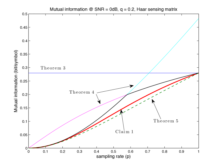
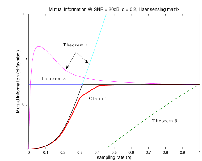
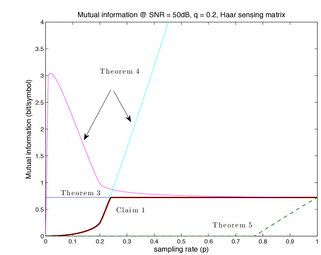
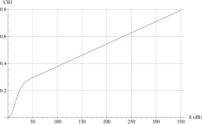
It is also interesting to observe that the asymptotic regime of vanishing $D(p,q,{\cal P}_{x})$ for any $p>q$ is approached very slowly, i.e., an impractically high SNR is required. For example, we notice that at ${\sf SNR}=50$ dB the mutual information ${\cal I}$ in Fig. 3 achieves the upper upper bound of Theorem 3 (very close to $h(q)$) at $p=0.24$, which is quite far from the threshold $q=0.2$. Fig. 4 shows ${\cal I}_{\rm ub}$ evaluated at $q=0.2,p=0.205$ versus SNR in dB. In order to reach the value $h(q)=0.722$ bits, we need an SNR of about 340 dB. This gives an idea of “how high” the high-SNR regime must be, in order to work closely to the noiseless reconstruction threshold.

Figure 4: Mutual information upper bound (right-hand side of (68)) versus ${\sf SNR}=q{\cal P}_{x}$ (dB), for $q=0.2$ and $p=0.205$.

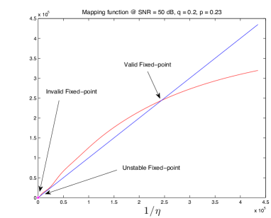
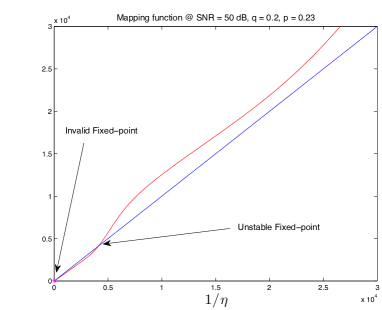
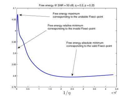
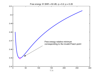
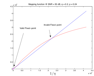
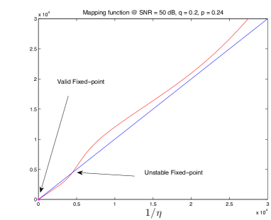
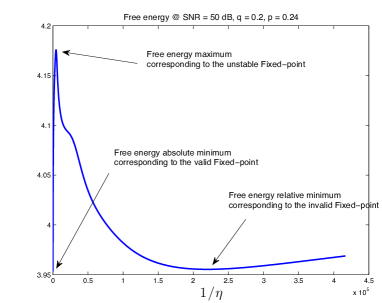
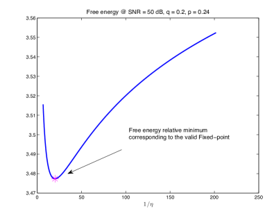
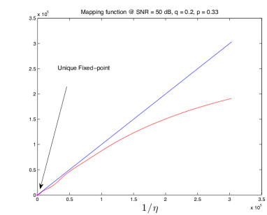
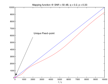
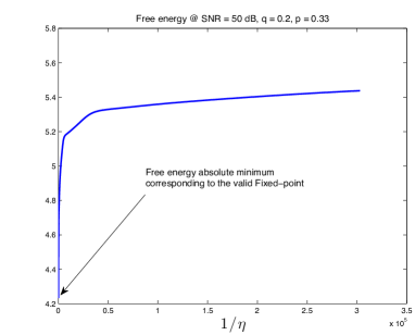
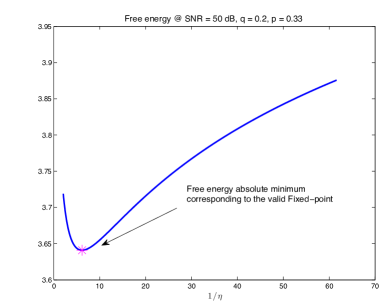
Next, we take a closer look at the behavior of the solutions of the fixed-point equation (17a) – (17b). Even in the iid case (in which the equation reduces to (25)) solved in [18, 28], the question of how to choose among the multiple solutions has not been thoroughly addressed in the literature. Fig. 5, 6 and 7 show the fixed-point mapping function obtained by eliminating $\chi$ from (17a) – (17b), and given by

$$f(1/\eta)=\frac{1}{\mathcal{R}_{{\bf R}}\left(-{\sf mmse}\left(V_{0}|V_{0}+\eta^{-\frac{1}{2}}Z\right)\right)},$$ (80)

given as a function of $1/\eta$, for $q=0.2$ and ${\sf SNR}=50$ dB. The intersections of this function with the main diagonal are the solutions of the equation $1/\eta=f(1/\eta)$. We explore the values of $p$ in the vicinity of the “phase transition” $p\approx 0.24$, for which the mutual information reaches a value very close to $h(q)$ (corresponding to $D(p,q,{\cal P}_{x})\approx 0$). For $p=0.23$ (see Fig. 5) we have three solutions. Two are stable fixed points and one is an unstable fixed point. The solution corresponding to the absolute minimum of the free energy ${\cal I}_{1}$ is the right-most fixed point (see Fig. 5(c)), corresponding to a large value of $1/\eta$, which in turn translates into a large support recovery error rate, as we will see in Section IV-F. For $p=0.24$ (see Fig. 6) we have also three solutions of which two are stable fixed points. However, now the solution corresponding to the absolute minimum of the free energy ${\cal I}_{1}$ is the left-most fixed point (see Fig. 6(c)), corresponding to a small value of $1/\eta$, i.e., to a very small support recovery error rate. This “jump” from the right-most to the left-most stable fixed point corresponds to a phase transition of the underlying statistical physics system. Notice that the phase transition may occur at finite SNR, as in this case, and the phase transition threshold $p^{*}$ is, in general, strictly larger than the noiseless perfect reconstruction threshold $q$. Finally, for values of $p$ significantly larger than the phase transition threshold (see the example for $p=0.33$ given in Fig. 7) only one solution exists. In this case, the free energy ${\cal I}_{1}$ has only one extremum point which is its absolute minimum (see Fig. 7(c)). For the Gaussian iid sensing matrix case it is known (see [31] and references therein) that the iterative algorithm known as AMP-MMSE achieves the right-most fixed point of (17a) – (17b). This coincides with the optimal MAP-SBS performance when this is the valid fixed point, corresponding to the minimum of ${\cal I}_{1}$. Instead, when there are multiple fixed points and the left-most fixed point is the valid one, the MAP-SBS estimator is strictly better than AMP-MMSE. Our results lead us to believe that the same behavior holds for a more general class of sensing matrices, as studied in this paper. From the examples above we notice that the right-most fixed point is the valid one for $p$ below the phase transition threshold. Above that threshold, either there is only one fixed point, for sufficiently large $p$, or one has to choose the solution that minimizes the free energy.

(a) Mapping function

(b) Detail near $1/\eta=0$

(c) Free energy

(d) Free energy detail near $1/\eta=0$

Figure 5: (a) Mapping function for the fixed-point equation (17a) – (17b) for $q=0.2$, $p=0.23$ and ${\sf SNR}=50$ dB. (b) Detail in order to evidence the unstable fixed point and the left-most fixed point. (c) Corresponding free energy. (d) Detail of the free energy for small $1/\eta$ in order to show the minimum corresponding to the left-most fixed point.

(a) Mapping function

(b) Detail near $1/\eta=0$

(c) Free energy

(d) Free energy detail near $1/\eta=0$

Figure 6: (a) Mapping function for the fixed-point equation (17a) – (17b) for $q=0.2$, $p=0.24$ and ${\sf SNR}=50$ dB. (b) Detail in order to evidence the unstable fixed point and the left-most fixed point. (c) Corresponding free energy. (d) Detail of the free energy for small $1/\eta$ in order to show the minimum corresponding to the left-most fixed point.

(a) Mapping function

(b) Detail near $1/\eta=0$

(c) Free energy

(d) Free energy detail near $1/\eta=0$

Figure 7: (a) Mapping function for the fixed-point equation (17a) – (17b) for $q=0.2$, $p=0.33$ and ${\sf SNR}=50$ dB. (b) Corresponding free energy. (d) Detail of the free energy for small $1/\eta$ in order to show the minimum corresponding to the left-most fixed point.

IV Analysis of Estimators using the Decoupling Principle

IV-A Decoupling principle

The decoupling principle introduced by Guo and Verdú [18] states that the marginal joint distribution of each input coordinate and the corresponding estimator coordinate of a class of, possibly mismatched, posterior-mean estimators (PMEs) converges, as the dimension grows, to a fixed input-output joint distribution that corresponds to a “decoupled” (i.e., scalar) Gaussian observation model. The observation model treated by Guo and Verdú in [18] is ${\bf y}={\bf S}\hbox{\boldmath$\Gamma$}{\bf x}+{\bf z}$, and the goal is to estimate ${\bf x}$ from ${\bf y}$, while knowing ${\bf S}$ and $\Gamma$, where ${\bf x}$ is an $m\times 1$ iid vector with a given marginal distribution, ${\bf z}$ is the iid Gaussian noise vector, ${\bf S}$ is a random $n\times m$ matrix with iid elements with mean zero and variance $1/n$, and $\Gamma$ is an $m\times m$ diagonal matrix whose diagonal elements have an empirical distribution converging weakly to a given well-behaved distribution. Comparing the model of [18] with (1), we notice that as far as the estimation of the Bernoulli-Gaussian iid vector ${\bf v}={\bf X}{\bf b}$ the two models are similar, by identifying ${\bf S}$ with ${\bf A}{\bf U}$, $\Gamma$ with ${\bf I}$ and ${\bf x}$ with ${\bf v}$, with the key difference that we allow a more general class of matrices satisfying the freeness condition given at the beginning of Section I-A. In contrast, as far as the estimation of ${\bf b}$ is concerned, our model differs from [18] in that in our case the diagonal iid Gaussian matrix ${\bf X}$ is not known to the estimator.

In this section, we apply the decoupling principle to the estimation of ${\bf b}$ for the observation model (1). This allows us to derive the minimum possible support recovery error rate for any estimator, achieved by the MAP-SBS estimator. The details of the derivations are given in Appendix E, and the main results are summarized in the remainder of this section. We also consider linear MMSE and Lasso [36], two popular estimators in the compressed sensing literature. These estimators first produce an estimate of ${\bf v}$ and then recover an estimate of the support ${\bf b}$ by component wise thresholding. In order to analyze the suboptimal estimators, we resort to the decoupling principle for the estimation of ${\bf v}$, which can be derived along the same lines as Appendix E or, equivalently, by extending the analysis of [18] to the class of sensing matrices considered in this paper. In [31], linear MMSE and Lasso estimators are studied for the case of iid sensing matrices as special cases of the Approximated Message Passing (AMP) algorithm [11], the performance of which is rigorously characterized for ${\bf U}$ with iid Gaussian entries in the large dimensional limit through the solution of a state evolution equation [3]. The current AMP rigorous analysis does not go through for the more general class of matrices considered here. Therefore, we resort to the replica $+$ large deviation approach of Rangan, Fletcher and Goyal [28] in order to obtain the decoupled model corresponding to these estimators. Interestingly, when particularizing our results to the iid case, we recover the same AMP state evolution equations as given in [31].

For the sake of notation simplicity, we shall assume that all random variables and vectors appearing in the following formulas have a density (possibly including Dirac distributions), indicated by $p$ with the appropriate subscripts and arguments. In order to limit the proliferation of symbols, we use the same symbols to indicate random variables (or vectors) and the corresponding dummy arguments in the probability distributions.

The class of estimators for which the decoupling principle holds are mismatched PMEs where the mismatch is reflected in an assumed channel transition probability and symbol a priori probabilities that may not correspond to the actual ones. We shall reserve the letter $q$ with the appropriate subscripts and arguments to indicate these assumed distributions. The true conditional channel transition probability of ${\bf y}$ given ${\bf b},{\bf A},{\bf U},{\bf X}$ of (1) is given by (18). The corresponding assumed channel transition probability is given by

$$q_{{\bf y}|{\bf b},{\bf A},{\bf U},{\bf X}}({\bf y}|{\bf b},{\bf A},{\bf U},{\bf X})=\left(\frac{\gamma}{\pi}\right)^{n}\exp\left(-\gamma\left\|{\bf y}-{\bf A}{\bf U}{\bf X}{\bf b}\right\|^{2}\right),$$ (81)

where the assumed noise variance is $1/\gamma$ instead of 1. We let also $q_{{\bf b}}({\bf b})=\prod_{i=1}^{n}q_{b}(b_{i})$ denote an assumed a-priori distribution for ${\bf b}$, not necessarily Bernoulli-$q$. The mismatched estimator for ${\bf b}$ given ${\bf y},{\bf A},{\bf U}$ is given by The corresponding PME takes on the form

$$\widehat{{\bf b}}({\bf y},{\bf A},{\bf U})=\int{\bf b}\;q_{{\bf b}|{\bf y},{\bf A},{\bf U}}({\bf b}|{\bf y},{\bf A},{\bf U})\;d{\bf b},$$ (82)

where

$$q_{{\bf b}|{\bf y},{\bf A},{\bf U}}({\bf b}|{\bf y},{\bf A},{\bf U})=\frac{\int q_{{\bf y}|{\bf b},{\bf A},{\bf U},{\bf X}}({\bf y}|{\bf b},{\bf A},{\bf U},{\bf X})q_{{\bf b}}({\bf b})p_{{\bf x}}({\bf x})d{\bf x}}{\int q_{{\bf y}|{\bf b},{\bf A},{\bf U},{\bf X}}({\bf y}|{\bf b}^{\prime},{\bf A},{\bf U},{\bf X})q_{{\bf b}}({\bf b}^{\prime})p_{{\bf x}}({\bf x})d{\bf x}d{\bf b}^{\prime}},$$ (83)

and where $p_{{\bf x}}({\bf x})=\frac{1}{(\pi{\cal P}_{x})^{n}}\exp(-\|{\bf x}\|^{2}/{\cal P}_{x})$ is the $n$-variate iid Complex Gaussian density with components $\sim{\cal C}{\cal N}(0,{\cal P}_{x})$.

In the matched case, for $\gamma=1$ and $q_{{\bf b}}({\bf b})\equiv$ Bernoulli-$q$, (82) coincides with the MMSE estimator.  By considering general $\gamma$ and $q_{{\bf b}}({\bf b})$, we can study of a whole family of mismatched PMEs through the same unified framework [35, 18].

For the purpose of analysis, it is convenient to define a virtual multivariate observation model involving the random vectors ${\bf b}_{0}\sim p_{{\bf b}_{0}}({\bf b}_{0})$, Bernoulli-$q$, the corresponding observation channel output ${\bf y}={\bf A}{\bf U}{\bf X}{\bf b}_{0}+{\bf z}$ as in (1), and an intermediate vector ${\bf b}\sim q_{{\bf b}}({\bf b})$, not corresponding to any physical quantity present in the original model, such that the conditional joint distribution of ${\bf b}_{0},{\bf y},{\bf b}$ given ${\bf A},{\bf U}$ is given by

$$p_{{\bf b}_{0}}({\bf b}_{0})\ p_{{\bf y}|{\bf b}_{0},{\bf A},{\bf U}}({\bf y}|{\bf b}_{0},{\bf A},{\bf U})\ q_{{\bf b}|{\bf y},{\bf A},{\bf U}}({\bf b}|{\bf y},{\bf A},{\bf U}),$$ (84)

with

$$p_{{\bf y}|{\bf b}_{0},{\bf A},{\bf U},{\bf X}}({\bf y}|{\bf b}_{0},{\bf A},{\bf U},{\bf X})=\frac{1}{\pi^{n}}\exp\left(-\left\|{\bf y}-{\bf A}{\bf U}{\bf X}{\bf b}_{0}\right\|^{2}\right).$$ (85)

Then, $\widehat{{\bf b}}({\bf y},{\bf A},{\bf U})$ can be seen as the “matched” PME of ${\bf b}$ given ${\bf y}$ with respect to the joint probability distribution (84). Notice also that (84) satisfies the conditional Markov Chain ${\bf b}_{0}\rightarrow{\bf y}\rightarrow{\bf b}$, for given ${\bf A},{\bf U}$.

The decoupling principle obtained in this paper and proved in Appendix E can be stated as follows. Let $(b_{0i},b_{i},\widehat{b}_{i})$ denote the $i$-th components of the random vectors ${\bf b}_{0},{\bf b},\widehat{{\bf b}}({\bf y},{\bf A},{\bf U})$, obeying the joint conditional distribution (84) with $\widehat{{\bf b}}({\bf y},{\bf A},{\bf U})$ given in (82). Then, in the limit of $n\rightarrow\infty$, under the assumption that the replica-symmetric analysis holds (see Appendix E), the joint distribution of $(b_{0i},b_{i},\widehat{b}_{i})$ converges to the joint distribution of the triple $(B_{0},B,\widehat{B})$ induced by

$$p_{B_{0}}(b_{0})\ p_{Y|B_{0};\eta}(y|b_{0})\ q_{B|Y;\xi}(b|y),$$ (86)

and by $\widehat{B}=\int b\;q_{B|Y;\xi}(b|y)db$, where we define the decoupled channel

$$Y=V_{0}+\eta^{-\frac{1}{2}}Z,$$ (87)

with $Z\sim{\cal C}{\cal N}(0,1)$ and $V_{0}=X_{0}B_{0}$, with $B_{0}\sim p_{B_{0}}(b_{0})$, Bernoulli-$q$, and with $X_{0}\sim{\cal C}{\cal N}(0,{\cal P}_{x})$, and where $X_{0},B_{0}$ and $Z$ are mutually independent. Also, we define $V=XB$ with $X\sim{\cal C}{\cal N}(0,{\cal P}_{x})$ and $B\sim q_{B}(b)$ identically distributed as the the marginals of the assumed prior distribution $q_{{\bf b}}({\bf b})$. We let $p_{X}(\cdot)$ denote the common density of $X_{0}$ and $X$, and define the following probability densities for the variables $V_{0},Y,V,B_{0}$ and $B$:

$$p_{Y|V_{0};\eta}(y|v_{0}) = \frac{\eta}{\pi}\exp\left(-\eta\left|y-v_{0}\right|^{2}\right)$$ (88)

$$p_{Y|B_{0};\eta}(y|b_{0}) = \int p_{Y|V_{0};\eta}(y|x_{0}b_{0})p_{X}(x_{0})dx_{0}$$ (89)

$$q_{Y|V;\xi}(y|v) = \frac{\xi}{\pi}\exp\left(-\xi\left|y-v\right|^{2}\right)$$ (90)

$$q_{Y|B;\xi}(y|b) = \int q_{Y|V;\xi}(y|xb)p_{X}(x)dx$$ (91)

$$q_{B|Y;\xi}(b|y) = \frac{q_{Y|B;\xi}(y|b)q_{B}(b)}{\int q_{Y|B;\xi}(y|b^{\prime})q_{B}(b^{\prime})db^{\prime}},$$ (92)

where the parameters $\eta$ and $\xi$ are obtained by solving the system of fixed-point equations

$$\chi = \gamma\,{\mathsf{mmse}}(V|Y)$$ (93a)

$$\delta = \mbox{\bb E}\left[|V_{0}-\mbox{\bb E}[V|Y]|^{2}\right]$$ (93b)

$$\xi = \gamma\,{\cal R}_{{\bf R}}(-\chi)$$ (93c)

$$\eta = \frac{(\xi/\gamma)^{2}}{\xi/\gamma+\dot{{\cal R}}_{{\bf R}}(-\chi)(\delta-\chi)}.$$ (93d)

The expectations in (93a) – (93d) are defined with respect to the joint distribution of $V_{0},Y,V$ given by

$$p_{V_{0}}(v_{0})\ p_{Y|V_{0};\eta}(y|v_{0})\ q_{V|Y;\xi}(v|y),$$ (94)

where $p_{V_{0}}(v_{0})$ is the Bernoulli-Gaussian distribution of $V_{0}=X_{0}B_{0}$, $p_{Y|V_{0};\eta}(y|v_{0})$ is given in (88) and where

$$q_{V|Y;\xi}(v|y)=\frac{q_{Y|V;\xi}(y|v)q_{V}(v)}{q_{Y;\xi}(y)},$$ (95)

with $q_{Y|V;\xi}(y|v)$ given in (90), $q_{V}(v)$ is the distribution of $V=XB$, and

$$q_{Y;\xi}(y)=\int q_{Y|V;\xi}(y|v)q_{V}(v)dv.$$ (96)

In passing, notice also that (86) and (94) satisfy the Markov Chains $B_{0}\rightarrow Y\rightarrow B$ and $V_{0}\rightarrow Y\rightarrow V$, respectively.

If the solution to (93a) – (93d) is not unique, then we have to select the solution that minimizes the system “free energy” (expressed in nats):

$${\cal E} =\log\frac{\xi}{\gamma}-\frac{\xi}{\eta}+\gamma-\xi\chi+\left(\frac{\xi}{\eta}-1\right)\frac{\xi\chi}{\gamma}+\int_{0}^{\chi}{\cal R}_{{\bf R}}(-w)dw-\mbox{\bb E}\left[\log\left(q_{Y;\xi}(Y)\right)\right].$$ (97)

As expected, by letting $\gamma=1$ and $q_{B}(b)$ Bernoulli-$q$ we obtain $\xi=\eta$ and $\delta=\chi$ and (93a) – (93d) reduce to (17a) – (17b). It is also immediate to see that in this case we have ${\cal E}={\cal I}_{1}+\log(\pi e)$ where ${\cal I}_{1}$ is given in (16).

By particularizing our analysis to the case of ${\bf U}$ with iid elements, using (24), we obtain the simpler fixed-point equations

$$\frac{1}{\eta} = \frac{1}{p}\left(1+\mbox{\bb E}\left[|V_{0}-\mbox{\bb E}[V|Y]|^{2}\right]\right)$$ (98a)

$$\frac{1}{\xi} = \frac{1}{p}\left(\frac{1}{\gamma}+{\mathsf{mmse}}(V|Y)\right),$$ (98b)

which recovers the results of [18, 28, 15] up to a different normalization as discussed in the first example of Section II-D.

IV-B Symbol-by-symbol MAP estimator

As an application of the decoupling principle, we can determine the minimum achievable $D(p,q,{\cal P}_{x})$ by particularizing the above formulas for the MAP-SBS estimator of $b_{i}$ given ${\bf y},{\bf A},{\bf U}$, operating according to the optimal decision rule

$$\widehat{b}_{i}({\bf y},{\bf A},{\bf U})={\hbox{arg}}\max_{b\in\{0,1\}}\mbox{\bb P}[b_{i}=b|{\bf y},{\bf A},{\bf U}].$$ (99)

It is well-known that the MAP-SBS minimizes the support recovery error rate over all possible estimators. A byproduct of the decoupling principle is that, in the matched case, (86) yields immediately that the limiting posterior marginal $\mbox{\bb P}[b_{i}=b|{\bf y},{\bf A},{\bf U}]$ for a randomly chosen $i$-th component of ${\bf b}$ is given by $p_{B_{0}|Y;\eta}(b_{0}|y)$, the posterior distribution of the decoupled channel (87), marginalized with respect to $B_{0}$. In the matched case, (93a) – (93d) reduce to (17a) – (17b) in Theorem 1, and $p_{B_{0}|Y;\eta}(b_{0}|y)$ is easily obtained by noticing that $Y$ given $B_{0}$ is conditionally distributed as

$$p_{Y|B_{0};\eta}(y|b_{0})=\frac{1}{\pi({\cal P}_{x}|B_{0}|^{2}+1/\eta)}\exp\left(-\frac{|y|^{2}}{{\cal P}_{x}|B_{0}|^{2}+1/\eta}\right),$$ (100)

i.e., $Y\sim{\cal C}{\cal N}\left(0,{\cal P}_{x}+1/\eta\right)$ for $B_{0}=1$ and $Y\sim{\cal C}{\cal N}\left(0,1/\eta\right)$ for $B_{0}=0$. Then,

$$\mbox{\bb P}[B_{0}=1|Y=y]=\frac{1}{1+\frac{1-q}{q}(1+\eta{\cal P}_{x})\exp\left(-\eta{\cal P}_{x}\mu|y|^{2}\right)},$$ (101)

(obviously $\mbox{\bb P}[B_{0}=0|Y=y]=1-\mbox{\bb P}[B_{0}=1|Y=y]$) where $\eta$ is obtained from (17a) – (17b) and where we define:

$$\mu=\frac{\eta}{1+{\cal P}_{x}\eta}.$$ (102)

The resulting MAP-SBS estimator is

$$\widehat{B}(y)={\hbox{arg}}\max_{b_{0}\in\{0,1\}}\;\mbox{\bb P}[B_{0}=b_{0}|Y=y],$$ (103)

with decision $\widehat{B}(y)=1$ if

$$\frac{1-q}{q}(1+\eta{\cal P}_{x})\exp\left(-\eta{\cal P}_{x}\mu|y|^{2}\right)<1$$ (104)

(with randomization on the boundary). Taking the logarithm of both sides, we find the “energy detector” (analogous to non-coherent on-off modulation with fading) given by

$$\widehat{B}(y)=\left\{\begin{array}[]{ll}1,&\mbox{for}\;|y|^{2}\geq\tau\\ 0,&\mbox{elsewhere}\end{array}\right.$$ (107)

with

$$\tau=\frac{1}{\eta{\cal P}_{x}\mu}\log\frac{(1-q)(1+\eta{\cal P}_{x})}{q}.$$ (108)

We have $\widehat{B}(y)=1$, regardless of the value of $y\in\mbox{\bb C}$, if $q>\frac{1+\eta{\cal P}_{x}}{2+\eta{\cal P}_{x}}$, in which case $D(p,q,{\cal P}_{x})=1-q$. Otherwise,

$$D(p,q,{\cal P}_{x})=q\left(1-\exp\left(-\mu\tau\right)\right)+(1-q)\exp\left(-\eta\tau\right),$$ (109)

obtained from (107) by observing that $|Y|^{2}$, conditioned on $B_{0}$, is central chi-square with two degrees of freedom with mean ${\cal P}_{x}+1/\eta$ for $B_{0}=1$ and with mean $1/\eta$ for $B_{0}=0$.

For ${\bf U}$ with iid elements, we can recover known results. In this case, (17a) – (17b) reduce to (25), which corresponds to the replica analysis of the MMSE estimator obtained in [18] and summarized in [31] in the context of support recovery in compressed sensing. When the iterative solution of the fixed-point equation (25) is initialized by $1/\eta=(1+q{\cal P}_{x})/p$, then the iteration converges to the solution of the so-called “AMP-MMSE” state equation given in [31, Th. 6]. In brief, by this initialization the iterative solution converges always to the right-most fixed point of the mapping function (see Figs. 5 – 7 and related discussion). Instead, if the valid fixed-point is chosen, i.e., the solution which minimizes the free energy ${\cal I}_{1}$, then we obtain the so-called “replica MMSE solution” of [31, Th. 8].

Next, we discuss the threshold for perfect support reconstruction in the noiseless case, i.e., in the limit of ${\cal P}_{x}\rightarrow\infty$, and $q>0$. From Theorem 6 we already know that vanishing $D(p,q,{\cal P}_{x})$ cannot be achieved for any $p\leq q$. We now show that $D(p,q,{\cal P}_{x})$ vanishes for large ${\cal P}_{x}$ for all $p>q$. This has previously been shown for both optimal nonlinear measurement schemes and for Gaussian iid sensing matrices in [43]. Therefore, the conclusion about the asymptotic optimality of Gaussian iid sensing matrices found in [43] extends to sparsely sampled free random matrices. We start by recalling the following general result from [42]:

Theorem 7

Let $V$ is a discrete-continuous mixed distribution, i.e. such that its distribution can be represented as

$$\nu=(1-\rho)\nu_{d}+\rho\nu_{c},$$ (110)

where $\nu_{d}$ is a discrete distribution and $\nu_{c}$ is an absolutely continuous distribution, and $0\leq\rho\leq 1$. Then, for $Z\sim{\cal C}{\cal N}(0,1)$ we have

$${\mathsf{mmse}}(V|\sqrt{{\sf snr}}{V}+Z)=\frac{\rho}{{\sf snr}}+o\left(\frac{1}{{\sf snr}}\right).$$ (111)

∎

We are interested in the behavior of the SNR of the decoupled channel (87) resulting from the MAP-SBS estimator, given by $q\,\eta\,{\cal P}_{x}$, as ${\cal P}_{x}\rightarrow\infty$. In particular, for given sparsity $0<q\leq 1$, we are interested in determining the range of sampling rates $p$ for which $q\,\eta\,{\cal P}_{x}\rightarrow\infty$, implying that $D(p,q,{\cal P}_{x})\rightarrow 0$. Let $Z$ and $V_{0}$ be as defined in Claim 1. Then, using Theorem 7 we can write

$${\mathsf{mmse}}\left(V_{0}|V_{0}+\eta^{\frac{1}{2}}Z\right) = {\cal P}_{x}\;{\mathsf{mmse}}\left(V_{0}/\sqrt{{\cal P}_{x}}|\sqrt{{\cal P}_{x}\eta}V_{0}/\sqrt{{\cal P}_{x}}+Z\right)$$ (112)

$$= \frac{q}{\eta}+o\left(1\right),$$ (113)

where, for the time being, we assume that ${\cal P}_{x}\eta$ grows unbounded as ${\cal P}_{x}\rightarrow\infty$. Using (113) into (17a) – (17b), for sufficiently large ${\cal P}_{x}$ we have

$$\eta = {\cal R}_{{\bf R}}(-{\mathsf{mmse}}(V_{0}|V_{0}+\eta^{\frac{1}{2}}{Z}))$$ (114)

$$\rightarrow {\cal R}_{{\bf R}}\left(-\frac{q}{\eta}\right).$$ (115)

For the case of ${\bf U}$ with iid elements, using (24) we obtain

$${\cal R}_{{\bf R}}^{-1}(z)=1-\frac{p}{z}$$ (116)

and solving (115) with respect to $\eta$, we obtain

$$\eta=p-q.$$ (117)

In the case of Haar-distributed ${\bf U}$, using (36), we obtain

$${\cal R}_{{\bf R}}^{-1}(z) = \frac{p-z}{(1-z)z}$$ (118)

$$\eta = \frac{p-q}{1-q}$$ (119)

For $p>q$, in those two cases the solutions are strictly positive and, consequently, the support recovery error rate vanishes as the SNR grows without bound. In fact, as we show next, this conclusion holds for the general class of sparsely sample free random matrices.

The goal is to show that $\lim_{{\cal P}_{x}\rightarrow\infty}\eta>0$ for $p>q$, without relying on a closed-form expression for the R-transform. This implies that $D(p,q,{\cal P}_{x})$ vanishes for large ${\cal P}_{x}$ for all $p>q$. Assuming that (115) holds, using the definition of the R-transform as function of the $\eta$-transform given in [38, Eq. 2.75 Sec. 2.2.5] and the definition of $\eta$-transform as given in [38, Sec. 2.2.2], we can rewrite the asymptotic equality $\eta={\cal R}_{{\bf R}}(-q/\eta)$ as:

$$q = 1-\mbox{\bb E}\left[\frac{1}{1+s|{\sf R}|^{2}}\right]$$ (120)

where $s$ satisfies

$$\frac{q}{\eta}=\mbox{\bb E}\left[\frac{s}{1+s|{\sf R}|^{2}}\right]$$ (121)

and $|{\sf R}|^{2}$ denotes a random variable distributed as the limiting spectrum of ${\bf R}$.

By eliminating $q$ and solving for $\eta$ in (120), (121) we obtain

$$\eta=\frac{\mbox{\bb E}\left[\frac{|{\sf R}|^{2}}{1+s|{\sf R}|^{2}}\right]}{\mbox{\bb E}\left[\frac{1}{1+s|{\sf R}|^{2}}\right]}.$$ (122)

It is immediate to see that (122) is strictly positive for any finite $s$ (ranging from the mean to the harmonic mean of $|{\sf R}|^{2}$). In view of Property (268) of the $\eta$-transform,

$$1-p\leq\mbox{\bb E}\left[\frac{1}{1+s|{\sf R}|^{2}}\right]\leq 1,$$ (123)

we conclude that (120) admits a unique positive and finite solution $s$ if and only if $1-q\in(1-p,1]$, i.e., for $p>q$. Hence, (122) yields $\eta>0$ for ${\cal P}_{x}\rightarrow\infty$, as we wanted to show.

We conclude this section by providing expressions for the MMSE in the estimation of the Bernoulli-Gaussian signal ${\bf v}$ for high SNR. For iid ${\bf U}$, we have

$${\mathsf{mmse}}\left(V_{0}|V_{0}+\eta^{\frac{1}{2}}Z\right) = -{\cal R}_{{\bf R}}^{-1}(\eta)$$ (124)

$$= \frac{p}{\eta}-1,$$ (125)

while for Haar-distributed ${\bf U}$, we have

$${\mathsf{mmse}}\left(V_{0}|V_{0}+\eta^{\frac{1}{2}}Z\right) = -{\cal R}_{{\bf R}}^{-1}(\eta)$$ (126)

$$= \frac{p-\eta}{(1-\eta)\eta}.$$ (127)

Notice that (125) coincides with the result derived in [43] and that the high-SNR MMSE diverges for $p=q$. Since deleting samples cannot improve the performance of the optimal MMSE estimator, it diverges for all $0\leq p\leq q$.

IV-C Replica analysis of a class of estimators via the large-deviation limit

The classical noisy compressed sensing problem seeks the estimation of the sparse vector ${\bf v}={\bf X}{\bf b}$ from ${\bf y}$ in (1) for known ${\bf A},{\bf U}$. Then, ${\bf b}$ can be estimated by componentwise thresholding the estimate of ${\bf v}$.

A number of suboptimal low-complexity estimators in the compressed sensing literature take on the form

$$\widehat{{\bf v}}={\hbox{arg}}\min_{{\bf v}\in\mbox{\bb C}^{n}}\left\{\gamma\left\|{\bf y}-{\bf A}{\bf U}{\bf v}\right\|^{2}+\sum_{i=1}^{n}f(v_{i})\right\},$$ (128)

for some weighting parameter $\gamma>0$ and cost function $f:\mbox{\bb C}\rightarrow\mbox{\bb R}_{+}$.

The replica decoupling principle can be used to study the large-dimensional limit performance of such class of estimators by following the large-deviation recipe given in [28]. Briefly, the approach of [28] considers a sequence of mismatched PMEs indexed by a parameter $\kappa\in\mbox{\bb R}_{+}$, where the assumed a priori density for ${\bf v}$ takes on the form

$$q^{(\kappa)}_{{\bf v}}({\bf v})=\frac{\exp\left(-\kappa\sum_{i=1}^{n}f(v_{i})\right)}{\int\exp\left(-\kappa\sum_{i=1}^{n}f(z_{i})\right)d{\bf z}},$$ (129)

(assuming that the integral converges for sufficiently large $\kappa$), and where the assumed transition density is given by

$$q^{(\kappa)}_{{\bf y}|{\bf v},{\bf A},{\bf U}}({\bf y}|{\bf v},{\bf A},{\bf U})=\left(\frac{\gamma\kappa}{\pi}\right)^{n}\exp\left(-\gamma\kappa\left\|{\bf y}-{\bf A}{\bf U}{\bf v}\right\|^{2}\right).$$ (130)

Under a number of mild technical assumptions (see [28] for details), $\widehat{{\bf v}}$ in (128) can be obtained as the limit of the PME

$$\widehat{{\bf v}}^{(\kappa)}=\int{\bf v}q^{(\kappa)}_{{\bf v}|{\bf y},{\bf A},{\bf U}}({\bf v}|{\bf y},{\bf A},{\bf U})d{\bf v}.$$ (131)

for $\kappa\rightarrow\infty$. Furthermore, for $n\rightarrow\infty$ and assuming the validity of the replica analysis, a decoupled scalar channel model in the limit of $\kappa\rightarrow\infty$ can be established such that the joint distribution of $(v_{0i},v_{i},\widehat{v}_{i})$ converges to the joint distribution of $(V_{0},V,\widehat{V})$, where the form of the joint distribution of $V_{0},Y,V$ is again given by (94) and where $\widehat{V}$ is a function of $Y$. The form of the fixed-point equations yielding $\eta$ and $\xi$ and of $\widehat{V}$ as a function of $Y$ depend on the specific estimator considered, i.e., on the value of $\gamma$ and on the cost function $f(v)$ in (128). In particular, following in the footsteps of [28] with a few minor variations in order to adapt to our case,  it is not difficult to show that $\widehat{V}=\widehat{v}(Y;\xi)$, where we define

$$\widehat{v}(y;\xi)={\hbox{arg}}\min_{v\in\mbox{\bb C}}\left\{\xi|y-v|^{2}+f(v)\right\},$$ (132)

and that the fixed-point equations yielding $\eta$ and $\xi$ in the limit of $\kappa\rightarrow\infty$ are given by

$$\chi = \gamma\mbox{\bb E}\left[\sigma^{2}(Y;\xi)\right]$$ (133a)

$$\delta = \mbox{\bb E}\left[|V_{0}-\widehat{v}(Y;\xi)|^{2}\right]$$ (133b)

$$\xi = \gamma{\cal R}_{{\bf R}}(-\chi)$$ (133c)

$$\eta = \frac{(\xi/\gamma)^{2}}{\xi/\gamma+\dot{{\cal R}}_{{\bf R}}(-\chi)(\delta-\chi)},$$ (133d)

where

$$\sigma^{2}(y;\xi)=\lim_{v\rightarrow\widehat{v}(y;\xi)}\frac{|v-\widehat{v}(y;\xi)|^{2}}{\xi|y-v|^{2}+f(v)-\left[\xi|y-\widehat{v}(y;\xi)|^{2}+f(\widehat{v}(y;\xi))\right]},$$ (134)

When ${\bf U}$ has iid elements, from (98a) – (98b) we find

$$\frac{1}{\eta} = \frac{1}{p}\left(1+\mbox{\bb E}\left[|V_{0}-\widehat{v}(Y;\xi)|^{2}\right]\right)$$ (135a)

$$\frac{1}{\xi} = \frac{1}{p}\left(\frac{1}{\gamma}+\mbox{\bb E}\left[\sigma^{2}(Y;\xi)\right]\right),$$ (135b)

which coincide with [28, Eq. (30a) - (30b)], up to a different normalization and the fact that we consider complex circularly symmetric instead of real random variables as in [28].

IV-D Thresholded linear MMSE estimator

A simple suboptimal estimator for ${\bf v}$ is the linear MMSE estimator, given by

$$\widehat{{\bf v}}=\left[\gamma^{-1}{\bf I}+{\bf R}\right]^{-1}{\bf U}^{\dagger}{\bf A}^{\dagger}{\bf y}.$$ (136)

with $\gamma=q{\cal P}_{x}$ and ${\bf R}$ defined in (3). It is immediate to verify that (136) can be expressed in the form (128) by letting $f(v)=|v|^{2}$.

Although the asymptotic performance and the decoupled channel model of linear MMSE estimation can be obtained directly from classical results in large random matrix theory both for iid and for Haar-distributed ${\bf U}$ (see [38] and references therein), it is instructive to apply the replica large-deviation approach outlined before. In this way, we can recover known results obtained rigorously by other means, thus lending support to the validity of the replica-based large-deviation approach.

Particularizing (132) and (134) to the case $f(v)=|v|^{2}$ we obtain

$$\widehat{v}(y;\xi)=\frac{\xi}{1+\xi}y$$ (137)

and

$$\sigma^{2}(y;\xi)=\frac{1}{1+\xi},$$ (138)

yielding

$$\mbox{\bb E}\left[|V_{0}-\widehat{v}(Y;\xi)|^{2}\right] = \mbox{\bb E}\left[\left|V_{0}-\frac{\xi}{1+\xi}Y\right|^{2}\right]$$ (139)

$$= \frac{\gamma+\xi^{2}/\eta}{(1+\xi)^{2}},$$ (140)

where we used the fact that $\mbox{\bb E}[|V_{0}|^{2}]=q{\cal P}_{x}=\gamma$. Replacing (138) and (140) into (133a) – (133d), we obtain the fixed-point equations for the linear MMSE estimator. In the iid case, using (135a) – (135b), we obtain that $\xi=\gamma\eta$ and

$$\eta=\frac{-(1+(1-p)\gamma)+\sqrt{(1+(1-p)\gamma)^{2}+4p\gamma}}{2\gamma},$$ (141)

which coincides with the well-known expression of the multiuser efficiency of the linear MMSE detector for an iid matrix with aspect ratio $pn\times n$ and elements with mean 0 and variance $1/n$ (see [38] and expression (54) evaluated for $\beta=1,s=\gamma$).

In the Haar-distributed case, using (36), we can solve explicitly for $\xi$ by eliminating $\chi$ in (133a) and (133c). After some more complicated algebra than in the iid case, we arrive at the solution

$$\xi=\frac{\gamma p}{1+(1-p)\gamma}$$ (142)

We also find that, as in the iid case, $\xi=\gamma\eta$. Hence $\eta$ is given in closed form as

$$\eta=\frac{p}{1+(1-p)\gamma},$$ (143)

which coincides with the well-known form of the multiuser efficiency of the linear MMSE detector for a CDMA system with observation model ${\bf r}={\bf A}{\bf U}{\bf v}+{\bf z}$, where ${\bf U}$ is $n\times n$ Haar-distributed, given by the solution of (55) in the case $\beta=1,s=\gamma$ (or, equivalently, by the limit of (56) for $\beta\rightarrow 1$).

In order to calculate the performance of the thresholded linear MMSE estimator, notice that the estimator output converges in distribution to $\widehat{V}=\widehat{v}(Y;\xi)=\frac{\xi}{1+\xi}Y$ where, according to the decoupled channel model, $Y=V_{0}+\eta^{-\frac{1}{2}}Z$, and $Z\sim{\cal C}{\cal N}(0,1)$. Thresholding $\widehat{V}$ or $Y$ is clearly equivalent. Hence, the support recovery error rate in this case takes on the same form already derived for the MAP-SBS (see (107) – (109)), for a different value of $\eta$ calculated via (133a) – (133d).

IV-E Thresholded Lasso estimator

We now follow an approach similar to that in Section IV-D in order to analyze the Lasso estimator, which so far has only been analyzed for iid sensing matrices.

The Lasso estimator, widely studied in the compressed sensing literature [44, 9] comes directly in the form (128) for $f(v)=|v|$. In this case, the parameter $\gamma$ must be optimized depending on the target performance. For example, in the classical noisy compressed sensing problem we are interested in the value of $\gamma$ that minimizes $\mbox{\bb E}[\|{\bf v}-\widehat{{\bf v}}\|^{2}]$.

Particularizing (132) and (134) to the case $f(v)=|v|$ we obtain

$$\widehat{v}(y;\xi)=\left[|y|-\frac{1}{2\xi}\right]_{+}\frac{y}{|y|},$$ (144)

where $[\cdot]_{+}$ takes the positive part of its argument, and

$$\sigma^{2}(y;\xi)=1\left\{|y|-\frac{1}{2\xi}>0\right\}\frac{1}{\xi},$$ (145)

where $1\{\cdot\}$ is the indicator function of the event inside the brackets. Notice that (144) and (145) generalize the expressions found in [28] to the complex case. In this case, we have

$$\mbox{\bb E}\left[|V_{0}-\widehat{v}(Y;\xi)|^{2}\right] = \mbox{\bb E}\left[\left|V_{0}-\left[|Y|-\frac{1}{2\xi}\right]_{+}\frac{Y}{|Y|}\right|^{2}\right]$$ (146)

$$= q{\cal P}_{x}+\frac{1-q}{\eta}\left[e^{-\eta^{\prime}}-\sqrt{\pi\eta^{\prime}}{\rm erfc}\left(\sqrt{\eta^{\prime}}\right)\right]$$

$$+\frac{q}{\mu}\left[\frac{1-{\cal P}_{x}\eta}{1+{\cal P}_{x}\eta}e^{-\mu^{\prime}}-\frac{\sqrt{\pi\mu^{\prime}}}{1+{\cal P}_{x}\eta}{\rm erfc}\left(\sqrt{\mu^{\prime}}\right)\right],$$

where $\eta^{\prime}=\eta/(4\xi^{2})$, $\mu^{\prime}=\mu/(4\xi^{2})$, and $\mu$ is defined in (102). The derivation of (146) is not completely straightforward and it is provided in Appendix H.

From (145) we have

$$\mbox{\bb E}[\sigma^{2}(Y;\xi)] = \frac{1}{\xi}\mbox{\bb P}[|Y|>1/(2\xi)]$$ (147)

$$= \frac{1}{\xi}\left(qe^{-\mu^{\prime}}+(1-q)e^{-\eta^{\prime}}\right)$$ (148)

Replacing (146) and (147) into (133a) – (133d), we obtain the fixed-point equation for calculating the decoupled channel parameters $\eta,\xi$ for the analysis of the Lasso estimator for given parameter $\gamma$. In the iid case, using (135a) – (135b), we obtain the same system of equations given in [28], up to a different normalization and the fact that here we consider complex signals. Furthermore, it is immediate to recognize that (135a) corresponds to the state evolution of the AMP with soft-thresholding (AMP-ST) as described in [31], where the scalar soft-thresholding function is given by (144) for an arbitrary thresholding parameter $\xi>0$. The large-dimensional analysis leading to the state evolution equation (135a) is rigorously proved in [3] for the case where ${\bf U}$ is iid Gaussian. Based on this fact, it is tempting to conjecture that the analysis is valid for the general iid case (subject to usual mild conditions on the matrix element distribution) and that the replica analysis yields correct results also for the more general class of matrices considered in this paper.

In order to obtain an estimate of ${\bf b}$ (support of ${\bf v}$), a natural approach consists of selecting the non-zero components of $\widehat{{\bf v}}$. However, this method yields rather poor results in the Bernoulli-Gaussian case and in other cases where the magnitudes of the non-zero components of ${\bf v}$ are not bounded away from zero. Instead, in an iterative implementation of the Lasso solver (e.g., using the method in [45], or the AMP-ST), it is possible to generate a “noisy” version of the Lasso estimate $\widehat{{\bf v}}$ before the soft-thresholding step (see Section IV-F and [31]). This noisy Lasso estimate corresponds to the decoupled channel model with marginal distribution $Y=V_{0}+\eta^{-\frac{1}{2}}Z$, with $\eta$ given by the fixed-point equation in the Lasso case. Hence, the support recovery error rate takes on the same form already derived for the MAP-SBS (see (107) – (109)), for a different value of $\eta$, calculated via (133a) – (133d) for the Lasso case as explained above.

IV-F Support recovery error rate examples

In order to illustrate the above results and compare the behavior of different support estimators, we show some numerical examples and compare the theoretical asymptotic results with finite-dimensional simulations. Figs. 8 and 9 show the support recovery error rate $D(p,q,{\cal P}_{x})$ versus the sampling rate $p$ for a Haar-distributed sensing matrix ${\bf U}$ and a Gaussian-Bernoulli source signal ${\bf v}$ with $q=0.2$ and ${\sf SNR}=q{\cal P}_{x}$ equal to $20$ and 50 dB, respectively.

Figure 8: Support recovery error rate $D(p,q,{\cal P}_{x})$ versus $p$, for $q=0.2$ and ${\sf SNR}=q{\cal P}_{x}=20$ dB for different estimators, asymptotic results and and finite-dimensional simulations. Solid thick line: MAP-SBS, asymptotic; Dotted line: Information theoretic lower bound; Dot-dash line: Thresholded Lasso, asymptotic; Dashed line: Thresholded linear MMSE, asymptotic; Thin solid line: Conjectured AMP-MMSE, corresponding to the right-most fixed point of (17a) – (17b). Some finite-dimensional simulations are shown for dimension $n=100$ for the thresholded linear MMSE estimator (asterisk: Haar sensing matrix; triangle: DFT sensing matrix) and for the thresholded Lasso (lozenge: Haar sensing matrix; star: DFT sensing matrix).

Figure 9: Support recovery error rate $D(p,q,{\cal P}_{x})$ versus $p$, for $q=0.2$ and ${\sf SNR}=q{\cal P}_{x}=50$ dB for different estimators, asymptotic results and and finite-dimensional simulations. Solid thick line: MAP-SBS, asymptotic; Dotted line: Information theoretic lower bound; Dot-dash line: thresholded Lasso, asymptotic; Dashed line: Thresholded linear MMSE, asymptotic; Thin solid line: Conjectured AMP-MMSE, corresponding to the right-most fixed point of (17a) – (17b). Some finite-dimensional simulations are shown for dimension $n=100$ for the thresholded linear MMSE estimator (asterisk: Haar sensing matrix; triangle: DFT sensing matrix) and for the thresholded Lasso (lozenge: Haar sensing matrix; star: DFT sensing matrix).

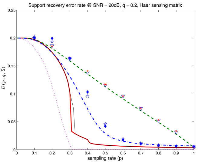
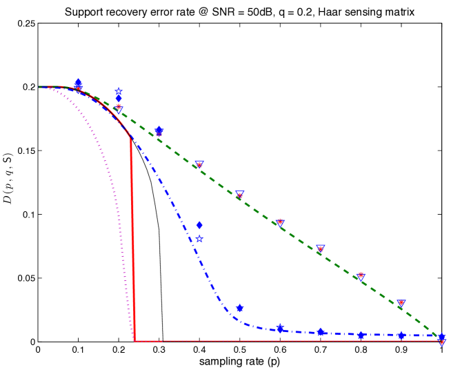
A few remarks are in order:

• The MAP-SBS asymptotic distortion is obtained by choosing the fixed-point solution of (17a) – (17b) that minimizes the free energy ${\cal I}_{1}$, as discussed in Section III-D. Instead, if we choose only the right-most fixed point, we obtain the solution of the conjectured state evolution equation corresponding to the AMP-MMSE applied to Haar-distributed sensing matrices. As previously remarked, it is known that such state evolution equation is exact in the case of iid sensing matrices.

• The information theoretic lower bound is obtained by taking the minimum of all the upper bounds on ${\cal I}$ developed in Theorems 48 and 4, and using it in (14).

• We run finite-dimensional simulations for dimension $n=100$ for the thresholded linear MMSE and thresholded Lasso estimators. We considered both random unitary ${\bf U}$ (Haar distributed) and the case of a fixed deterministic ${\bf U}={\bf F}$, where ${\bf F}$ is the $n$-dimensional unitary DFT matrix with elements $[{\bf F}]_{m,k}=\frac{e^{j\frac{2\pi}{n}(m-1)(k-1)}}{\sqrt{n}}$. Interestingly, the simulations show that random unitary and deterministic DFT yields essentially the same performance (up to Monte Carlo simulation fluctuations). This corroborates our conjecture that the asymptotic analysis of Haar-distributed ${\bf U}$ carries over to the case of a DFT matrix. The case of DFT matrices is particularly relevant for applications, since in many communication and signal processing problems signals are sparse in the time (resp., frequency) domain and are randomly sampled in the dual domain, so that a random selection of the rows of a DFT matrix arises as a sensing matrix naturally matched to the problem.

• As already noticed in several works, the gap between the optimal MAP-SBS estimator and the suboptimal low-complexity estimators grows for high SNR (compare Fig. 8 and Fig. 9). In contrast, the thresholded linear MMSE estimator yields poor performance for all $p<1$, and this is quite insensitive to SNR.

• In order to solve the complex Lasso, we used the iterative method of [45]. This scheme has slightly lower complexity than AMP-ST, and provably converges to the Lasso solution. By comparing the component-wise thresholding step in [45] and the symbol-by-symbol estimator $\hat{v}(Y;\xi)$ for the decoupled channel model given in (144), it is natural to identify the noisy Lasso solution with the vector

  $$\widetilde{{\bf v}}=\widehat{{\bf v}}^{(\infty)}+{\bf D}{\bf G}^{\dagger}\left({\bf y}-{\bf G}\widehat{{\bf v}}^{(\infty)}\right),$$ (149)

  where $\widehat{{\bf v}}^{(\infty)}$ is the solution of the iterative algorithm of [45] after convergence, ${\bf G}$ is the matrix obtained by taking the non-zero rows of ${\bf A}{\bf U}$, and ${\bf D}={\hbox{diag}}(1/\|{\bf g}_{1}\|^{2},\ldots,1/\|{\bf g}_{n}\|^{2})$ where ${\bf g}_{\ell}$ is the $\ell$-th column of ${\bf G}$. The support recovery error rate shown in Figs. 8 and 9 for the finite-dimensional simulation of the thresholded Lasso is obtained by applying the threshold detector given in (107), for $\eta$ calculated via the asymptotic fixed-point equations (133a) – (133d), to the components of $\widetilde{{\bf v}}$ given in (149). The asymptotic analysis and the finite-dimensional simulation were computed for the same value of the parameter $\gamma$, which must be chosen for each combination of system parameters $p,q$ and ${\cal P}_{x}$. Several heuristic methods for the choice of $\gamma$ are proposed in the literature. Following [46], we used $\gamma=(1/20)\|{\bf G}^{\dagger}{\bf y}\|_{\infty}$ (the optimization of $\gamma$ for the asymptotic case is an interesting topic for further investigation.)

V Conclusion

In the standard compressed sensing model, the sensing matrix ${\bf A}{\bf U}$ is such that ${\bf A}$ is diagonal with independent $\{0,1\}$ components and ${\bf U}$ has iid coefficients. In addition to this model, we allow the square matrix ${\bf U}$ to be Haar-distributed (uniformly distributed among all unitary matrices) or, more generally, to be free from any Hermitian deterministic matrix.

Motivated by applications, in this paper we have carried out a large-size analysis of:

1. the mutual information between the noisy observations and the Bernoulli-Gaussian input (conditioned on the sensing matrix),

2. the mutual information between the noisy observations and the Gaussian input prior to being subject to random “hole-punching”.

We have obtained asymptotic formulas using fundamentally different approaches for both mutual informations: the first following a replica-method analysis whose scope we enlarge to encompass the desired class of random matrices, while the second invokes results from freeness and the asymptotic spectral distribution of random matrices.

Depending on the case, the mutual informations are expressed either through the mutual information between a scalar Bernoulli-Gaussian random variable and its Gaussian-contaminated version, or explicitly, through the solution of coupled nonlinear equations. We have also studied how to choose among the solutions of those equations.

Our upper and lower bounds on the mutual informations do not rely on the replica method. Yet, they turn out to give excellent agreement with the replica analysis. Through the analysis of the bounds we also provide a simple converse which shows that the asymptotic distortion is bounded away from zero regardless of signal-to-noise ratio for $p\leq q$. For $p>q$, Wu and Verdú [43] showed that Gaussian iid sensing matrices are asymptotically as effective for compressed sensing as the best nonlinear measurement (or encoder). Here, we have been able to extend that conclusion to the class of sparsely sampled free random matrices.

We have analyzed several decision rules such as the optimum symbol-by-symbol rule, the Lasso, and the linear MMSE estimator, followed by thresholding for support recovery. Those analyses follow the decoupling principle, originally introduced in [18] for iid matrices. Specializing these new results we recover the iid formulas found in [18, 28, 31], with the exception of the ML detector analyzed in [31], which is tailored to the case when the number of nonzero coefficients is known at the estimator, while in our analysis that number is binomially distributed.

The important case where ${\bf U}$ is a deterministic DFT matrix remains open. However, we have provided intuition and simulation evidence to buttress the conjecture that its solution in fact coincides with the case where ${\bf U}$ is Haar distributed.

Acknowledgements

G. Caire, S. Shamai, and S. Verdú wish to acknowledge the Binational Science Foundation Grant N. 2008269. The work of G. Caire was partially supported by NSF Grant CCF-0729162. The work of S. Verdú was partially supported by the Center for Science of Information (CSoI), an NSF Science and Technology Center, under grant agreement CCF-0939370.

Appendix A Proof of Theorem 1

Let $(X,Y)\sim P_{X}P_{Y|X}$. For any $\widehat{X}\in\widehat{{\cal X}}$, such that $X\leftrightarrow Y\leftrightarrow\widehat{X}$, and function $\mathsf{d}\colon{\cal X}\times\widehat{{\cal X}}\rightarrow[0,\infty)$, (12) and the data processing inequality yield

$$R(\mathbb{E}[\mathsf{d}(X,\widehat{X})]) \leq I(X;\widehat{X})$$ (150)

$$\leq I(X;Y)$$ (151)

Supremizing over $\widehat{X}$ and in view of the fact that $R(\cdot)$ is a monotonically non-increasing function, the result follows.

It is worth emphasizing the totally elementary nature of the proof of Theorem 1, and in particular the fact that it does not involve any type of operational characterization of information theoretic fundamental coding limits. A different approach based on those limits and Fano’s inequality is taken in [31] to show Lemma 5 therein.

Appendix B Proof of Claim 1

We let ${\bf v}_{0}={\bf X}{\bf b}_{0}$ with ${\bf X}{\hbox{diag}}({\bf x})$ and ${\bf x}$ an iid Gaussian vector with $p_{\bf x}({\bf x})=\frac{1}{(\pi{\cal P}_{x})^{n}}\exp\left(-\|{\bf x}\|^{2}/{\cal P}_{x}\right)$ and ${\bf b}_{0}$ Bernoulli-$q$, with probability mass function $p_{{\bf b}_{0}}({\bf b}_{0})$. Notations are as in Section IV-A). In particular, ${\bf y}={\bf A}{\bf U}{\bf X}{\bf b}_{0}+{\bf z}$, as in (1). Consider the assumed conditional probability density

$$q_{{\bf y}|{\bf v},{\bf A},{\bf U}}({\bf y}|{\bf v},{\bf A},{\bf U})=\left(\frac{\gamma}{\pi}\right)^{n}\exp\left(-\gamma\left\|{\bf y}-{\bf A}{\bf U}{\bf v}\right\|^{2}\right)$$ (152)

for some $\gamma>0$. We also consider an assumed iid prior density on ${\bf v}$, denoted by $g({\bf v})$ for simplicity of notation, and let $g_{0}({\bf v}_{0})$ denote the Bernoulli-Gaussian density of ${\bf v}_{0}$. Removing the conditioning with respect to ${\bf v}$, we obtain

$$q_{{\bf y}|{\bf A},{\bf U}}({\bf y}|{\bf A},{\bf U})=\left(\frac{\gamma}{\pi}\right)^{n}\int g({\bf v})\exp\left(-\gamma\left\|{\bf y}-{\bf A}{\bf U}{\bf v}\right\|^{2}\right)d{\bf v}.$$ (153)

We wish to calculate the mutual information rate ${\cal I}_{1}$ defined in (8), which can be expressed as

$${\cal I}_{1} = \lim_{n\rightarrow\infty}\frac{1}{n}I({\bf v}_{0};{\bf y}|{\bf A},{\bf U})$$ (154)

$$= \lim_{n\rightarrow\infty}\frac{1}{n}\left[-\mbox{\bb E}[\log p_{{\bf y}|{\bf A},{\bf U}}({\bf y}|{\bf A},{\bf U})]+\mbox{\bb E}[\log p_{{\bf y}|{\bf v}_{0},{\bf A}{\bf U}}({\bf y}|{\bf v}_{0},{\bf A},{\bf U})]\right]$$ (155)

$$= -\lim_{n\rightarrow\infty}\frac{1}{n}\left.\mbox{\bb E}[\log Z({\bf y},{\bf A},{\bf U})]\right|_{\stackrel{{\scriptstyle g(\cdot)=g_{0}(\cdot)}}{{\gamma=1}}}-\log(\pi e)$$ (156)

where we define $Z({\bf y},{\bf A},{\bf U})=q_{{\bf y}|{\bf A},{\bf U}}({\bf y}|{\bf A},{\bf U})$, and recognize that (153) can be interpreted as the partition function (from which the notation “$Z$”) of a statistical mechanical system with “quenched disorder parameters” ${\bf y},{\bf A},{\bf U}$, “state” ${\bf v}\sim g(\cdot)$ and unnormalized Boltzman distribution $q_{{\bf y}|{\bf v},{\bf A},{\bf U}}({\bf y}|{\bf v},{\bf A},{\bf U})g({\bf v})$. 

The condition $g(\cdot)=g_{0}(\cdot 0$ and $\gamma=1$ correspond to the case where the assumed prior and noise variance in the observation model are “matched”, i.e., they coincide with the true priors and noise variance. However, it is useful to consider the derivation for general $\gamma$ and $g(\cdot)$, since this same derivation will apply to the general class of mismatched PMEs defined in Section IV-A). The quantity

$${\cal E}=-\lim_{n\rightarrow\infty}\frac{1}{n}\mbox{\bb E}[\log Z({\bf y},{\bf A},{\bf U})]$$ (157)

is the system per-component free-energy of the underlying physical system. In the following, we shall compute ${\cal E}$ using the Replica Method of statistical physics, under the so-called Replica Symmetry (RS) assumption [26, 25, 35, 18, 17]. Summarizing, the method comprises the following steps: since computing the expectation of the log in (157) is usually complicated, we use the identity

$$\mbox{\bb E}[\log Z({\bf y},{\bf A},{\bf U})]=\lim_{u\rightarrow 0}\frac{\partial}{\partial u}\log\left(\mbox{\bb E}\left[Z^{u}({\bf y},{\bf A},{\bf U})\right]\right)$$ (158)

for $u\in\mbox{\bb R}_{+}$. Then, exchanging limits, we can write

$${\cal E}=-\lim_{u\rightarrow 0}\frac{\partial}{\partial u}\lim_{n\rightarrow\infty}\frac{1}{n}\log\left(\mbox{\bb E}\left[Z^{u}({\bf y},{\bf A},{\bf U})\right]\right)$$ (159)

Finally, we evaluate the quantity

$$\lim_{n\rightarrow\infty}\frac{1}{n}\log\left(\mbox{\bb E}\left[Z^{u}({\bf y},{\bf A},{\bf U})\right]\right)$$ (160)

for $u$ positive integer, such that $Z^{u}({\bf y},{\bf A},{\bf U})$ can be seen as the partition function of a $u$-fold Cartesian product system (i.e., $u$ parallel “replicas” of the original system), with state vectors ${\bf v}_{1},\ldots,{\bf v}_{u}$, and the same quenched parameters ${\bf y},{\bf A},{\bf U}$. In particular, we can write

$$Z^{u}({\bf y},{\bf A},{\bf U}) = \left(\frac{\gamma}{\pi}\right)^{un}\int d{\bf v}_{1}\cdots d{\bf v}_{u}\left(\prod_{a=1}^{u}g({\bf v}_{a})\right)\exp\left(-\gamma\sum_{a=1}^{u}\left\|{\bf y}-{\bf A}{\bf U}{\bf v}_{a}\right\|^{2}\right).$$ (161)

The next step consists of calculating

$$\mbox{\bb E}[Z^{u}({\bf y},{\bf A},{\bf U})|{\bf A},{\bf U}]=$$ (162)

$$=\left(\frac{\gamma}{\pi}\right)^{un}\int d{\bf v}_{0}d{\bf v}_{1}\cdots d{\bf v}_{u}\left(g_{0}({\bf v}_{0})\prod_{a=1}^{u}g({\bf v}_{a})\right)\;\int\exp\left(-\gamma\sum_{a=1}^{u}\left\|{\bf z}-{\bf A}{\bf U}({\bf v}_{a}-{\bf v}_{0})\right\|^{2}\right)\;\frac{1}{\pi^{n}}e^{-\|{\bf z}\|^{2}}\;d{\bf z}$$ (163)

Standard Gaussian integration (by completing the squares) yields

$$\int\exp\left(-\gamma\sum_{a=1}^{u}\left\|{\bf z}-{\bf A}{\bf U}({\bf v}_{a}-{\bf v}_{0})\right\|^{2}\right)\;\frac{1}{\pi^{n}}e^{-\|{\bf z}\|^{2}}\;d{\bf z} = (1+u\gamma)^{-n}\exp\left(-n{\hbox{tr}}\left({\bf R}{\bf L}\right)\right)$$ (164)

where ${\bf R}={\bf U}^{\dagger}{\bf A}^{\dagger}{\bf A}{\bf U}$, as defined in (3), and where ${\bf L}$ is a rank-$u$ matrix defined as follows: let ${\bf s}_{a}={\bf v}_{a}-{\bf v}_{0}$ for $a=1,\ldots,u$, and let ${\bf S}=[{\bf s}_{1},\ldots,{\bf s}_{u}]$. Then,

$${\bf L}=\frac{\gamma}{n}{\bf S}\left({\bf I}-\frac{1}{\gamma^{-1}+u}{\bf 1}{\bf 1}^{\sf T}\right){\bf S}^{\dagger}$$ (165)

where ${\bf 1}$ denotes an all-ones column vector of appropriate dimension. Next, we need to average with respect to ${\bf A},{\bf U}$, i.e., with respect to ${\bf R}$. To this purpose, we apply the generalized Harish-Chandra-Itzykson-Zuber integral [19, 21] as follows:

$$\lim_{n\rightarrow\infty}\frac{1}{n}\log\mbox{\bb E}[Z^{u}({\bf y},{\bf A},{\bf U})]=$$

$$=u\log\gamma-u\log\pi-\log(1+u\gamma)$$

$$+\lim_{n\rightarrow\infty}\frac{1}{n}\log\left(\int d{\bf v}_{0}\cdots d{\bf v}_{u}\left(g_{0}({\bf v}_{0})\prod_{a=1}^{u}g({\bf v}_{a})\right)\mbox{\bb E}\Big{[}\exp\left(-n{\hbox{tr}}\left({\bf R}{\bf L}\right)\right)\Big{|}{\bf L}\Big{]}\right)$$ (166)

$$=u\log\gamma-u\log\pi-\log(1+u\gamma)$$

$$+\lim_{n\rightarrow\infty}\frac{1}{n}\log\left(\int d{\bf v}_{0}\cdots d{\bf v}_{u}\left(g_{0}({\bf v}_{0})\prod_{a=1}^{u}g({\bf v}_{a})\right)\exp\left(-n\sum_{i=1}^{u}\int_{0}^{\lambda_{i}({\bf L})}{\cal R}_{{\bf R}}(-w)dw\right)\right)$$ (167)

where ${\cal R}_{{\bf R}}(w)$ denotes the R-transform of ${\bf R}$ and $\lambda_{(}{\bf L})$ denotes the $i$-th eigenvalue of ${\bf L}$.

Our goal now is to evaluate the limit

$$\lim_{n\rightarrow\infty}\frac{1}{n}\log\left(\int d{\bf v}_{0}\cdots d{\bf v}_{u}\left(g_{0}({\bf v}_{0})\prod_{a=1}^{u}g({\bf v}_{a})\right)\;\exp\left(-n\sum_{i=1}^{u}\int_{0}^{\lambda_{i}({\bf L})}{\cal R}_{{\bf R}}(-w)dw\right)\right).$$ (168)

In order to proceed, we make the common RS assumption and define the empirical correlations

$$Q_{a,a^{\prime}}=\frac{1}{n}\sum_{k=1}^{n}v_{ak}v^{*}_{a^{\prime}k}$$ (169)

of vectors ${\bf v}_{a},{\bf v}_{a^{\prime}}$ for $0\leq a,a^{\prime}\leq u$. Noticing that the limit (168) is given as the limit of a normalized log-sum, Varadhan’s lemma yields that this limit is given by the “dominant configuration” of the vectors ${\bf v}_{0},\ldots,{\bf v}_{u}$, defined in terms of their empirical correlation matrix ${\bf Q}=[Q_{a,a^{\prime}}]$. The RS assumption “postulates” that this dominant configuration satisfies the following symmetric form:

$${\bf Q}=\left[\begin{array}[]{cc}\epsilon_{0}&\vartheta{\bf 1}^{\sf T}\\ \vartheta^{*}{\bf 1}&(\epsilon_{1}-\omega){\bf I}+\omega{\bf 1}{\bf 1}^{\sf T}\end{array}\right].$$ (172)

In Appendix F we show that, for ${\bf Q}$ in the form (172), the eigenvalues of ${\bf L}$ are given by

$$\lambda_{1}\stackrel{{\scriptstyle\Delta}}{{=}}\lambda_{1}({\bf L}) = \frac{\epsilon_{1}-\omega+u(\epsilon_{0}-2{\rm Re}\{\vartheta\}+\omega)}{\gamma^{-1}+u}$$ (173)

$$\lambda_{2}\stackrel{{\scriptstyle\Delta}}{{=}}\lambda_{i}({\bf L}) = \gamma(\epsilon_{1}-\omega),\;\;\;\;i=2,\ldots,u$$ (174)

$$\lambda_{i}({\bf L}) = 0,\;\;\;\;i=u+1,\ldots,n.$$ (175)

Therefore, we define

$${\cal G}^{(u)}({\bf Q}) \stackrel{{\scriptstyle\Delta}}{{=}} \sum_{i=1}^{u}\int_{0}^{\lambda_{i}({\bf L})}{\cal R}_{{\bf R}}(-w)dw$$ (176)

$$= \int_{0}^{\lambda_{1}}{\cal R}_{{\bf R}}(-w)dw+(u-1)\int_{0}^{\lambda_{2}}{\cal R}_{{\bf R}}(-w)dw.$$ (177)

The argument of the logarithm in (168) can be interpreted as an expectation with respect to ${\bf v}_{0},\ldots,{\bf v}_{u}$, with joint pdf $g_{0}({\bf v}_{0})\prod_{a=1}^{u}g({\bf v}_{a})$. By the law of large numbers, this measure satisfies a concentration property with respect to the empirical correlations (169). Hence, we can invoke Cramér’s large deviation theorem [6] as follows. Since ${\bf Q}$ is a function of ${\bf v}_{0},\ldots,{\bf v}_{u}$, the conditional pdf of ${\bf Q}$ given ${\bf v}_{0},\ldots,{\bf v}_{u}$ is just a multi-dimensional delta function (i.e., a product of delta functions), hence, we can write

$$\int d{\bf v}_{0}\cdots d{\bf v}_{u}\left(g_{0}({\bf v}_{0})\prod_{a=1}^{u}g({\bf v}_{a})\right)\times\exp\left(-n{\cal G}^{(u)}({\bf Q})\right)$$ (178)

$$\;=\mbox{\bb E}\left[\int\exp\left(-n{\cal G}^{(u)}({\bf Q})\right)\mu_{n}^{(u)}(d{\bf Q}|{\bf v}_{0},\ldots,{\bf v}_{u})\right]$$ (179)

$$\;=\int\exp\left(-n{\cal G}^{(u)}({\bf Q})\right)\mu_{n}^{(u)}(d{\bf Q})$$ (180)

$$\;\approx\int\exp\left(-n\left({\cal G}^{(u)}({\bf Q})+I^{(u)}({\bf Q})\right)\right)d{\bf Q}$$ (181)

where (181) holds in the sense that, when we consider the quantity (180) inside the logarithm in the limit (168), it can be replaced by (181).

The rate function $I^{(u)}({\bf Q})$ of the measure $\mu^{(u)}_{n}(d{\bf Q})$ defined as

$$\mu_{n}^{(u)}(d{\bf Q}) = \int d{\bf v}_{0}\cdots d{\bf v}_{u}\left(g_{0}({\bf v}_{0})\prod_{a=1}^{u}g({\bf v}_{a})\right)\prod_{a\leq a^{\prime}}^{u}\delta\left(\sum_{k=1}^{n}v_{ak}v^{*}_{a^{\prime}k}-nQ_{a,a^{\prime}}\right)\;d{\bf Q}$$ (182)

$$= \mbox{\bb E}\left[\prod_{a\leq a^{\prime}}^{u}\delta\left(\sum_{k=1}^{n}v_{ak}v^{*}_{a^{\prime}k}-nQ_{a,a^{\prime}}\right)\right]\;d{\bf Q},$$ (183)

is given by the Legendre-Fenchel transform of the log-Moment Generating Function (log-MGF) of the random vector $\underline{{\bf V}}=(V_{0},V_{1},\ldots,V_{u})^{\sf T}$, where $V_{0}=X_{0}B_{0}$ and $V_{a}=X_{a}B_{a}$, $X_{0},X_{1},\ldots,X_{u}$ are iid Gaussian RVs $\sim p_{X}(x)=\frac{1}{\pi{\cal P}_{x}}\exp(-|x|^{2}/{\cal P}_{x})$, and $B_{0},B_{1},\ldots,B_{u}$ are independent variables with $B_{0}\sim p_{B_{0}}$ and $B_{a}\sim q_{B}$. The MGF of $\underline{{\bf V}}$ is given by

$$M^{(u)}(\tilde{{\bf Q}})=\mbox{\bb E}\left[\exp\left(\underline{{\bf V}}^{\dagger}\tilde{{\bf Q}}\underline{{\bf V}}\right)\right]$$ (184)

and the rate function is given by

$$I^{(u)}({\bf Q})=\sup_{\tilde{{\bf Q}}}\left\{{\hbox{tr}}(\tilde{{\bf Q}}{\bf Q})-\log M^{(u)}(\tilde{{\bf Q}})\right\}$$ (185)

Eventually, using this into (181) and the resulting expression in the limit (168) and applying Varadhan’s lemma, we arrive at the saddle-point condition

$$\lim_{n\rightarrow\infty}\frac{1}{n}\log\left(\int\mu^{(u)}_{n}(d{\bf Q})\exp\left(-n{\cal G}^{(u)}({\bf Q})\right)\right) = -\inf_{{\bf Q}}\left\{{\cal G}^{(u)}({\bf Q})+\sup_{\tilde{{\bf Q}}}\left\{{\hbox{tr}}(\tilde{{\bf Q}}{\bf Q})-\log M^{(u)}(\tilde{{\bf Q}})\right\}\right\}$$

$$= -\inf_{{\bf Q}}\sup_{\tilde{{\bf Q}}}\left\{{\cal G}^{(u)}({\bf Q})+{\hbox{tr}}(\tilde{{\bf Q}}{\bf Q})-\log M^{(u)}(\tilde{{\bf Q}})\right\}$$

Now we focus on the calculation of the MGF. Under the RS assumption, the supremum in (B) is achieved for $\tilde{{\bf Q}}$ in the form

$$\tilde{{\bf Q}}=\left[\begin{array}[]{cc}c&d{\bf 1}^{\sf T}\\ d^{*}{\bf 1}&(g-f){\bf I}+f{\bf 1}{\bf 1}^{\sf T}\end{array}\right]$$ (190)

where $c,d,g,f$ are parameters. Using the RS form for $\tilde{{\bf Q}}$ we obtain

$$M^{(u)}(\tilde{{\bf Q}})=\mbox{\bb E}\left[\exp\left(\left|\frac{d}{\sqrt{f}}V_{0}+\sqrt{f}\sum_{a=1}^{u}V_{a}\right|^{2}+\left(c-\frac{|d|^{2}}{f}\right)|V_{0}|^{2}+(g-f)\sum_{a=1}^{u}|V_{a}|^{2}\right)\right]$$ (191)

We use the complex circularly-symmetric version of the scalar Hubbard-Stratonovich transform [34, 20]:

$$e^{|x|^{2}}=\frac{\eta}{\pi}\int\exp\left(-\eta|z|^{2}+2\sqrt{\eta}{\rm Re}\{x^{*}z\}\right)dz$$ (192)

for $x,z\in\mbox{\bb C}$ and $\eta\in\mbox{\bb R}_{+}$. Choosing $\eta=|d|^{2}/f$, we obtain

$$\exp\left(\left|\frac{d}{\sqrt{f}}V_{0}+\sqrt{f}\sum_{a=1}^{u}V_{a}\right|^{2}\right) = \frac{|d|^{2}}{\pi f}\int\exp\left(-\frac{|d|^{2}}{f}|z|^{2}+2\frac{|d|}{\sqrt{f}}{\rm Re}\left\{\left(\frac{d}{\sqrt{f}}V_{0}+\sqrt{f}\sum_{a=1}^{u}V_{a}\right)^{*}z\right\}\right)dz$$

Using this into (191), after some straightforward algebra, we find

$$M^{(u)}(\tilde{{\bf Q}}) = \mbox{\bb E}\left[\frac{|d|^{2}}{\pi f}\int\exp\left(-\frac{|d|^{2}}{f}\left|z-(d/|d|)V_{0}\right|^{2}+c|V_{0}|^{2}\right)\exp\left(\sum_{a=1}^{u}\left(2|d|{\rm Re}\{V_{a}^{*}z\}+(g-f)|V_{a}|^{2}\right)\right)dz\right]$$

Notice that $V_{0}$ has a circularly symmetric distribution, therefore $(d/|d|)V_{0}$ and $V_{0}$ are identically distributed. Hence, we can write

$$M^{(u)}(\tilde{{\bf Q}}) = \mbox{\bb E}\left[\frac{|d|^{2}}{\pi f}\int\exp\left(-\frac{|d|^{2}}{f}\left|z-V_{0}\right|^{2}+c|V_{0}|^{2}\right)\exp\left(\sum_{a=1}^{u}\left(2|d|{\rm Re}\{V_{a}^{*}z\}+(g-f)|V_{a}|^{2}\right)\right)dz\right]$$

Since (B) depends only on $|d|$, without loss of generality we re-define the parameter $d$ to be in $\mbox{\bb R}_{+}$. Also, notice from (B) that $\lim_{u\rightarrow 0}M^{(u)}(\tilde{{\bf Q}})=1$.

Following the replica derivation steps outlined at the beginning of this section, we have to determine the saddle-point ${\bf Q}^{\star}(u)$ and $\tilde{{\bf Q}}^{\star}(u)$ achieving the extremal condition in (B), for general $u$, and finally replace the result in (B), differentiate with respect to $u$ and let $u\rightarrow 0$. Since the function in (B) is differentiable and admits a minimum and a maximum, following the result of Appendix G we have that determining the saddle-point $({\bf Q}^{\star}(u),\tilde{{\bf Q}}^{\star}(u))$, replacing it in (B), differentiating the resulting expression with respect to $u$ and letting $u\rightarrow 0$ yields the same result of replacing in (B) the saddle-point for $u=0$, denoted by ${\bf Q}^{\star}(0)={\bf Q}^{\star}$ and $\tilde{{\bf Q}}^{\star}(0)=\tilde{{\bf Q}}^{\star}$, differentiating the result with respect to $u$ and letting $u\rightarrow 0$, where now ${\bf Q}^{\star},\tilde{{\bf Q}}^{\star}$ are constants independent of $u$.

Differentiating (B) with respect to $\tilde{{\bf Q}}$, we obtain the equation

$${\bf Q}=\frac{\mbox{\bb E}\left[\underline{{\bf V}}\underline{{\bf V}}^{\dagger}\exp\left(\underline{{\bf V}}^{\dagger}\tilde{{\bf Q}}\underline{{\bf V}}\right)\right]}{\mbox{\bb E}\left[\exp\left(\underline{{\bf V}}^{\dagger}\tilde{{\bf Q}}\underline{{\bf V}}\right)\right]}$$ (196)

Since we evaluate the saddle-point conditions at $u\rightarrow 0$, and since the denominator in (196) is $M^{(u)}(\tilde{{\bf Q}})$, which is equal to 1 at $u\downarrow 0$, we can just disregard the denominator and focus on the numerator in the following. Using the expression (176) for ${\cal G}^{(u)}({\bf Q})$, with eigenvalues $\lambda_{1}$ and $\lambda_{2}$ given by (173), and noticing that the RS conditions (172) and (190) yield

$${\hbox{tr}}(\tilde{{\bf Q}}{\bf Q})=\epsilon_{0}c+u\epsilon_{1}g+2{\rm Re}\{\vartheta\}du+u(u-1)\omega f$$ (197)

we have that the whole exponent depends only on the real part of $\vartheta$. Therefore, we re-define $\vartheta$ to be a real parameter and differentiate with respect to $\vartheta$, $\omega$, $\epsilon_{1}$ and $\epsilon_{0}$, and impose that the partial derivatives are equal to zero. We find the conditions

$$d = \frac{1}{\gamma^{-1}+u}{\cal R}_{{\bf R}}(-\lambda_{1})$$ (198)

$$f = \frac{1}{u}\left(\gamma{\cal R}_{{\bf R}}(-\lambda_{2})-\frac{1}{\gamma^{-1}+u}{\cal R}_{{\bf R}}(-\lambda_{1})\right)$$ (199)

$$g-f = -\gamma{\cal R}_{{\bf R}}(-\lambda_{2})$$ (200)

$$c = -\frac{u}{\gamma^{-1}+u}{\cal R}_{{\bf R}}(-\lambda_{1})$$ (201)

Evaluating these conditions for $u\downarrow 0$ and noticing that, as $u$ vanishes, $\lambda_{1}\rightarrow\lambda_{2}$, we find:

$$d^{\star} = \gamma{\cal R}_{{\bf R}}(-\lambda^{\star}_{2})$$ (202)

$$f^{\star} = \lim_{u\rightarrow 0}\frac{1}{u}\left(\gamma{\cal R}_{{\bf R}}(-\lambda^{\star}_{2})-\frac{1}{\gamma^{-1}+u}{\cal R}_{{\bf R}}(-\lambda^{\star}_{1})\right)$$ (203)

$$= \left.-\frac{\partial}{\partial u}\left[\frac{1}{\gamma^{-1}+u}{\cal R}_{{\bf R}}(-\lambda^{\star}_{1})\right]\right|_{u=0}$$ (204)

$$= \gamma^{2}{\cal R}_{{\bf R}}(-\lambda^{\star}_{2})+\gamma^{2}\dot{{\cal R}}_{{\bf R}}(-\lambda^{\star}_{2})\left(\epsilon^{\star}_{0}-2\vartheta^{\star}+\omega^{\star}-\gamma(\epsilon^{\star}_{1}-\omega^{\star})\right)$$ (205)

$$g^{\star}-f^{\star} = -d^{\star}$$ (206)

$$c^{\star} = 0$$ (207)

where $\lambda_{2}^{\star}=\gamma(\epsilon_{1}^{\star}-\omega^{\star})$ and where $\dot{{\cal R}}_{{\bf R}}(\cdot)$ denotes the first derivative of ${\cal R}_{{\bf R}}(\cdot)$.

The conditions for $\epsilon_{0}^{\star},\epsilon_{1}^{\star},\vartheta^{\star},\omega^{\star}$ in terms of $d^{\star},g^{\star}$ and $f^{\star}$ are obtained from (196), recalling that, by definition, $\epsilon_{0}=Q_{00},\epsilon_{1}=Q_{11},\vartheta=Q_{01}$ and $\omega=Q_{12}$. In order to obtain more useful expressions for these parameters, we use (207) and (206) in (B) and write

$$M^{(u)}(\tilde{{\bf Q}}^{\star}) = \mbox{\bb E}\left[\frac{(d^{\star})^{2}}{\pi f^{\star}}\int\exp\left(-\frac{(d^{\star})^{2}}{f^{\star}}\left|z-V_{0}\right|^{2}\right)\exp\left(\sum_{a=1}^{u}\left(2d^{\star}{\rm Re}\{V_{a}^{*}z\}-d^{\star}|V_{a}|^{2}\right)\right)dz\right]$$ (209)

$$= \mbox{\bb E}\left[\frac{(d^{\star})^{2}}{\pi f^{\star}}\int\exp\left(-\frac{(d^{\star})^{2}}{f^{\star}}\left|z-V_{0}\right|^{2}\right)\exp\left(-d^{\star}\sum_{a=1}^{u}\left|z-V_{a}\right|^{2}\right)e^{d^{\star}u|z|^{2}}dz\right]$$

$$= \mbox{\bb E}\left[\frac{\eta}{\pi}\int\exp\left(-\eta\left|z-V_{0}\right|^{2}\right)\exp\left(-\xi\sum_{a=1}^{u}\left|z-V_{a}\right|^{2}\right)e^{\xi|z|^{2}u}dz\right]$$ (210)

where we define $\eta=(d^{\star})^{2}/f^{\star}$ and $\xi=d^{\star}$.

Focusing on the numerator in (196) and following steps similar to the derivation of (209), we obtain the following expressions for the correlation coefficients $\epsilon_{0},\vartheta,\epsilon_{1},\omega$:

1. For $\epsilon_{0}=Q_{00}$ we have

   $$\epsilon_{0}^{\star} = \mbox{\bb E}\Big{[}\int\frac{\eta}{\pi}|V_{0}|^{2}\exp\left(-\eta|z-V_{0}|^{2}\right)\cdot\exp\left(-\xi\sum_{a=1}^{u}|z-V_{a}|^{2}\right)\;e^{\xi|z|^{2}u}dz\Big{]}\Big{|}_{u\downarrow 0}$$ (212)

   $$= \mbox{\bb E}[|V_{0}|^{2}]$$ (213)

2. For $\vartheta=Q_{01}$, we introduce the RV $V\sim g(\cdot)$ (same distribution as any of the $V_{a}$’s) and independent of $V_{0},V_{1}$. Then, we can write

   $$\vartheta^{\star}=$$ (214)

   $$=\mbox{\bb E}\Big{[}\int\frac{\eta}{\pi}V_{0}\exp\left(-\eta|z-V_{0}|^{2}\right)\cdot V^{*}_{1}\exp\left(-\xi|z-V_{1}|^{2}\right)\cdot\exp\left(-\xi\sum_{a=2}^{u}|z-V_{a}|^{2}\right)\;e^{\xi|z|^{2}u}dz\Big{]}\Big{|}_{u\downarrow 0}$$ (215)

   $$=\mbox{\bb E}\Big{[}\int\frac{\eta}{\pi}V_{0}\exp\left(-\eta|z-V_{0}|^{2}\right)\cdot V^{*}_{1}\exp\left(-\xi|z-V_{1}|^{2}\right)\cdot\mbox{\bb E}\left[\exp\left(-\xi|z-V|^{2}\right)\right]^{u-1}\;e^{\xi|z|^{2}u}dz\Big{]}\Big{|}_{u\downarrow 0}$$ (216)

   $$=\mbox{\bb E}\Big{[}\int\frac{\eta}{\pi}V_{0}\exp\left(-\eta|z-V_{0}|^{2}\right)\cdot\mbox{\bb E}\left[\frac{V^{*}\exp\left(-\xi|z-V|^{2}\right)}{\mbox{\bb E}\left[\exp\left(-\xi|z-V|^{2}\right)\right]}\right]dz\Big{]}$$ (217)

3. For $\epsilon_{1}=Q_{11}$ we have:

   $$\epsilon_{1}^{\star}=$$ (218)

   $$=\mbox{\bb E}\Big{[}\int\frac{\eta}{\pi}\exp\left(-\eta|z-V_{0}|^{2}\right)\cdot|V_{1}|^{2}\exp\left(-\xi|z-V_{1}|^{2}\right)\cdot\exp\left(-\xi\sum_{a=2}^{u}|z-V_{a}|^{2}\right)\;e^{\xi|z|^{2}u}dz\Big{]}\Big{|}_{u\downarrow 0}$$ (219)

   $$=\mbox{\bb E}\Big{[}\int\frac{\eta}{\pi}\exp\left(-\eta|z-V_{0}|^{2}\right)\cdot|V_{1}|^{2}\exp\left(-\xi|z-V_{1}|^{2}\right)\cdot\mbox{\bb E}\left[\exp\left(-\xi|z-V|^{2}\right)\right]^{u-1}\;e^{\xi|z|^{2}u}dz\Big{]}\Big{|}_{u\downarrow 0}$$ (220)

   $$=\mbox{\bb E}\Big{[}\int\frac{\eta}{\pi}\exp\left(-\eta|z-V_{0}|^{2}\right)\cdot\mbox{\bb E}\left[\frac{|V|^{2}\exp\left(-\xi(z-V)^{2}\right)}{\mbox{\bb E}\left[\exp\left(-\xi|z-V|^{2}\right)\right]}\right]dz\Big{]}$$ (221)

4. For $\omega=Q_{12}$ we have:

   $$\omega^{\star}=$$ (222)

   $$=\mbox{\bb E}\Big{[}\int\frac{\eta}{\pi}\exp\left(-\eta|z-V_{0}|^{2}\right)V_{1}V^{*}_{2}\exp\left(-\xi|z-V_{1}|^{2}\right)\exp\left(-\xi|z-V_{2}|^{2}\right)\cdot$$ (223)

   $$\;\;\;\;\;\;\;\;\;\;\;\;\;\;\;\;\;\;\;\;\;\;\;\;\;\;\;\;\;\;\;\;\;\;\;\;\;\;\;\;\;\;\;\;\;\;\;\;\;\;\;\;\;\;\;\;\;\;\;\;\;\;\;\cdot\exp\left(-\xi\sum_{a=3}^{u}|z-V_{a}|^{2}\right)\;e^{\xi|z|^{2}u}dz\Big{]}\Big{|}_{u\downarrow 0}$$ (224)

   $$=\mbox{\bb E}\Big{[}\int\frac{\eta}{\pi}\exp\left(-\eta|z-V_{0}|^{2}\right)V_{1}V^{*}_{2}\exp\left(-\xi|z-V_{1}|^{2}\right)\exp\left(-\xi|z-V_{2}|^{2}\right)\cdot$$ (225)

   $$\;\;\;\;\;\;\;\;\;\;\;\;\;\;\;\;\;\;\;\;\;\;\;\;\;\;\;\;\;\;\;\;\;\;\;\;\;\;\;\;\;\;\;\;\;\;\;\;\;\;\;\;\;\;\;\;\;\;\;\;\;\;\;\cdot\mbox{\bb E}\left[\exp\left(-\xi|z-V|^{2}\right)\right]^{u-2}\;e^{\xi|z|^{2}u}dz\Big{]}\Big{|}_{u\downarrow 0}$$ (226)

   $$=\mbox{\bb E}\Big{[}\int\frac{\eta}{\pi}\exp\left(-\eta|z-V_{0}|^{2}\right)\cdot\left|\mbox{\bb E}\left[\frac{V\exp\left(-\xi|z-V|^{2}\right)}{\mbox{\bb E}\left[\exp\left(-\xi|z-V|^{2}\right)\right]}\right]\right|^{2}dz\Big{]}$$ (227)

Finally, we define a single-letter joint probability distribution and restate the expectations appearing in (214), (218), (222) in terms of this new single-letter model. Let $p_{V_{0}}(v_{0})$ denote the Bernoulli-Gaussian density of $V_{0}$, induced by $p_{X}(\cdot)$ and by $p_{B_{0}}(\cdot)$, and let

$$p_{Y|V_{0};\eta}(y|v_{0};\eta)=\frac{\eta}{\pi}\exp\left(-\eta|y-v_{0}|^{2}\right)$$ (228)

denote the transition probability density of the complex (scalar) circularly symmetric AWGN channel

$$Y=V_{0}+\eta^{-\frac{1}{2}}Z$$ (229)

with $Z\sim{\cal C}{\cal N}(0,1)$. Also, define the conditional complex circularly symmetric Gaussian pdf

$$q_{Y|V;\xi}(y|v;\xi)=\frac{\xi}{\pi}\exp\left(-\xi|y-v|^{2}\right)$$ (230)

and, using Bayes rule, consider the a-posteriori probability distribution

$$q_{V|Y;\xi}(v|y;\xi) = \frac{q_{Y|V;\xi}(y|v;\xi)g(v)}{\int q_{Y|V;\xi}(y|v;\xi)g(v)dv}$$ (231)

$$= \frac{\exp\left(-\xi|y-v|^{2}\right)g(v)}{\mbox{\bb E}\left[\exp\left(-\xi|y-V|^{2}\right)\right]}.$$ (232)

The joint single-letter probability distribution of interest for the variables $V_{0},Y$ and $V$ is given by

$$p_{V_{0}}(v_{0})p_{Y|V_{0};\eta}(y|v_{0};\eta)q_{V|Y;\xi}(v|y;\xi).$$ (233)

This explains the decoupled channel single-letter probability model (94).

Now, we can define the conditional mean of $V$ given $Y$ as

$$\mbox{\bb E}[V|Y=y] = \int v\;q_{V|Y;\xi}(v|y;\xi)dv$$ (234)

$$= \mbox{\bb E}\left[\frac{V\exp\left(-\xi|y-V|^{2}\right)}{\mbox{\bb E}\left[\exp\left(-\xi|y-V|^{2}\right)\right]}\right].$$ (235)

The corresponding conditional second moment is given by

$${\sf sm}_{V}(y;\xi) = \int|v|^{2}\;q_{V|Y;\xi}(v|y;\xi)dv$$ (236)

$$= \mbox{\bb E}\left[\frac{|V|^{2}\exp\left(-\xi|y-V|^{2}\right)}{\mbox{\bb E}\left[\exp\left(-\xi|y-V|^{2}\right)\right]}\right].$$ (237)

At this point, it is easy to identify the terms and write the expressions (214), (218), (222) in terms of expectations with respect to the single-letter joint probability measure defined in (233). We have

$$\epsilon_{0}^{\star} = \mbox{\bb E}[|V_{0}|^{2}]$$ (238)

$$\vartheta^{\star} = \mbox{\bb E}\left[V_{0}(\mbox{\bb E}[V|Y])^{*}\right]$$ (239)

$$\epsilon_{1}^{\star} = \mbox{\bb E}\left[{\sf sm}_{V}(Y;\xi)\right]$$ (240)

$$\omega^{\star} = \mbox{\bb E}\left[\left|\mbox{\bb E}[V|Y]\right|^{2}\right].$$ (241)

In order to obtain the desired fixed-points equations for the saddle-point that defines the result in (B), we notice that

$$\epsilon_{0}^{\star}-2\vartheta^{\star}+\omega^{\star}=\mbox{\bb E}\left[\left|V_{0}-\mbox{\bb E}[V|Y]\right|^{2}\right]$$ (242)

and that

$$\epsilon_{1}^{\star}-\omega^{\star} = \mbox{\bb E}\left[\left|V-\mbox{\bb E}[V|Y]\right|^{2}\right]$$ (243)

$$= {\sf mmse}(V|Y).$$ (244)

Using (198), (199), the equality $\lambda_{2}^{\star}=\gamma(\epsilon_{1}^{\star}-\omega^{\star})$, and recalling that $\xi=d^{\star}$ and $\eta=(d^{\star})^{2}/f^{\star}$, we arrive at the system of fixed-point equations (93a) – (93d). In the matched case, where $q_{B}(\cdot)=p_{B}(\cdot)$ and $\gamma=1$ we immediately obtain that $\delta=\chi$ and therefore $\xi=\eta$, and the fixed-point equations reduce to (17a) – (17b) in Claim 1.

Using the values solution of (93a) – (93d) into (B), using the trace expression (197) and finally putting everything together into (B) and taking the derivative w.r.t. $u$ evaluated at $u\downarrow 0$, we eventually obtain the free energy ${\cal E}$ in (157) as given by

$${\cal E} = \log(\pi/\gamma)+\gamma+\frac{\partial}{\partial u}\left.\left\{\int_{0}^{\lambda_{1}^{\star}}{\cal R}_{{\bf R}}(-w)dw+(u-1)\int_{0}^{\lambda_{2}^{\star}}{\cal R}_{{\bf R}}(-w)dw\right\}\right|_{u\downarrow 0}$$ (247)

$$+\left.\frac{\partial}{\partial u}\Big{\{}\epsilon^{\star}_{0}c^{\star}+u\epsilon^{\star}_{1}g^{\star}+2\vartheta^{\star}d^{\star}u+u(u-1)\omega^{\star}f^{\star}\Big{\}}\right|_{u\downarrow 0}$$

$$-\frac{\partial}{\partial u}\left.\log M^{(u)}(\tilde{{\bf Q}}^{\star})\right|_{u\downarrow 0}$$

Examining each term separately, we have:

$$\displaystyle{\frac{\partial}{\partial u}\left.\left\{\int_{0}^{\lambda_{1}^{\star}}{\cal R}_{{\bf R}}(-w)dw+(u-1)\int_{0}^{\lambda_{2}^{\star}}{\cal R}_{{\bf R}}(-w)dw\right\}\right|_{u\downarrow 0}}$$ (248)

$$=\displaystyle{\left.{\cal R}_{{\bf R}}(-\lambda_{1}^{\star})\frac{(\epsilon_{0}^{\star}-2\vartheta^{\star}+\omega^{\star})(\gamma^{-1}+u)-(\epsilon_{1}^{\star}-\omega^{\star}+u(\epsilon_{0}^{\star}-2\vartheta^{\star}+\omega^{\star}))}{(\gamma^{-1}+u)^{2}}\right|_{u\downarrow 0}+\int_{0}^{\lambda_{2}^{\star}}{\cal R}_{{\bf R}}(-w)dw}$$ (249)

$$=\displaystyle{\gamma{\cal R}_{{\bf R}}(-\lambda_{2}^{\star})\left(\epsilon_{0}^{\star}-2\vartheta^{\star}+\omega^{\star}-\gamma(\epsilon_{1}^{\star}-\omega^{\star})\right)+\int_{0}^{\lambda_{2}^{\star}}{\cal R}_{{\bf R}}(-w)dw}$$ (250)

$$=\displaystyle{\gamma{\cal R}_{{\bf R}}(-\chi)(\delta-\chi)+\int_{0}^{\chi}{\cal R}_{{\bf R}}(-w)dw}$$ (251)

where we have used the definition of $\chi$ and $\delta$ in (93a) and (93b), respectively, and the relations (242) and (243). For the trace term, recalling that $c^{\star}=0$, we have

$$\left.\frac{\partial}{\partial u}\Big{\{}\epsilon^{\star}_{0}c^{\star}+u\epsilon^{\star}_{1}g^{\star}+2\vartheta^{\star}d^{\star}u+u(u-1)\omega^{\star}f^{\star}\Big{\}}\right|_{u\downarrow 0} = \epsilon^{\star}_{1}g^{\star}+2\vartheta^{\star}d^{\star}-\omega^{\star}f^{\star}$$ (252)

Finally, for the log-MGF term we use (209) and performing the expectation with respect to $V_{1},\ldots,V_{u}$ (independent and identically distributed as $V$) first, we obtain

$$M^{(u)}(\tilde{{\bf Q}}^{\star}) = \mbox{\bb E}\left[\frac{\eta}{\pi}\int\exp\left(-\eta\left|z-V_{0}\right|^{2}\right)\left(\mbox{\bb E}\left[\exp\left(-\xi\left|z-V\right|^{2}\right)\right]e^{\xi|z|^{2}}\right)^{u}dz\right]$$ (253)

Hence,

$$-\frac{\partial}{\partial u}\left.\log M^{(u)}(\tilde{{\bf Q}}^{\star})\right|_{u\downarrow 0} = -\mbox{\bb E}\left[\frac{\eta}{\pi}\int\exp\left(-\eta\left|z-V_{0}\right|^{2}\right)\log\left(\mbox{\bb E}\left[\exp\left(-\xi\left|z-V\right|^{2}\right)\right]\right)dz\right]$$ (255)

$$-\xi\mbox{\bb E}\left[\frac{\eta}{\pi}\int|z|^{2}\exp\left(-\eta\left|z-V_{0}\right|^{2}\right)dz\right]$$

$$= -\mbox{\bb E}\left[\log\left(q_{Y;\xi}(Y)\right)\right]+\log\frac{\xi}{\pi}-\frac{\xi}{\eta}-\xi\mbox{\bb E}[|V_{0}|^{2}]$$ (256)

where in the last line we use (230) and define

$$q_{Y;\xi}(y) = \int q_{Y|V;\xi}(y|v)g(v)dv$$ (257)

$$= \frac{\xi}{\pi}\mbox{\bb E}\left[\exp\left(-\xi|y-V|^{2}\right)\right].$$ (258)

It is understood that if (93a) – (93d) have multiple solutions, then the solution that minimizes the free energy should be chosen.

We conclude by showing that (247) can be written in the form (97). Putting together (252) and the last term of (255) and recalling that $\mbox{\bb E}[|V_{0}|^{2}]=\epsilon^{\star}_{0}$ and that $\xi=d^{\star}$ we have:

$$\epsilon^{\star}_{1}g^{\star}+2\vartheta^{\star}d^{\star}-\omega f^{\star}-\epsilon^{\star}_{0}\xi=\epsilon^{\star}_{1}g^{\star}+2\vartheta^{\star}d^{\star}-\omega^{\star}f^{\star}-\epsilon_{0}^{\star}d^{\star}.$$ (259)

Adding and subtracting $\omega d^{\star}$ and using (242) and the definition of $\delta$ (see (93b)) we have

$$-\epsilon_{0}^{\star}d^{\star}+2\vartheta^{\star}d^{\star}-\omega^{\star}d^{\star}+\omega^{\star}d^{\star}-\omega^{\star}f^{\star}+\epsilon^{\star}_{1}g^{\star} = (-\epsilon_{0}^{\star}+2\vartheta^{\star}-\omega^{\star})d^{\star}+\omega^{\star}d^{\star}-\omega^{\star}f^{\star}+\epsilon^{\star}_{1}g^{\star}$$ (261)

$$= -\delta d^{\star}-\omega^{\star}(f^{\star}-d^{\star})+\epsilon^{\star}_{1}g^{\star}.$$

Recalling that $g^{\star}=f^{\star}-d^{\star}$, we obtain

$$-\delta d^{\star}+(\epsilon^{\star}_{1}-\omega^{\star})g^{\star}$$ (262)

Recalling that $\epsilon^{\star}_{1}-\omega^{\star}=\lambda^{\star}_{2}/\gamma=\chi/\gamma$, we get

$$-\delta d^{\star}+g^{\star}\chi/\gamma$$ (263)

Finally, using $d^{\star}=\xi$ and $\eta=(d^{\star})^{2}/f^{\star}$ we arrive at

$$-\delta\xi+d^{\star}(f^{\star}/d^{\star}-1)\chi/\gamma=-\delta\xi+d^{\star}((f^{\star}d^{\star})/(d^{\star})^{2}-1)\chi/\gamma=-\delta\xi+\xi(\xi/\eta-1)\chi/\gamma$$ (264)

Next, we use (264), the remaining terms of (255), (248) and the first terms in (247), together with the saddle-point equations (93a) – (93d), to eventually obtain ${\cal E}$ in the form (97).

For the case $q_{B}(\cdot)=p_{B}(\cdot)$ and $\gamma=1$, noticing that $\delta=\chi$ and $\xi=\eta$, with $\chi$ and $\eta$ given by (17a) – (17b), the free energy takes on the form

$${\cal E}=I\left(V_{0};V_{0}+\eta^{-\frac{1}{2}}Z\right)+\int_{0}^{\chi}\left({\cal R}_{{\bf R}}(-w)-\eta\right)dw+\log(e\pi),$$ (265)

where $Z\sim{\cal C}{\cal N}(0,1)$ and where we used the fact that when $\xi=\eta$ and $V\sim V_{0}$, then $q_{Y;\xi}(y)=p_{Y;\eta}(y)=\frac{\pi}{\eta}\mbox{\bb E}\left[\exp(-\eta(y-V_{0})^{2})\right]$, so that

$$-\mbox{\bb E}\left[\log q_{Y;\xi}(Y)\right]-\log\frac{e\pi}{\xi}=h\left(V_{0}+\eta^{-\frac{1}{2}}Z\right)-h\left(\eta^{-\frac{1}{2}}Z\right)=I\left(V_{0};V_{0}+\eta^{-\frac{1}{2}}Z\right).$$ (266)

Using (265) in the mutual information expression (156) we obtain (16) in Claim 1.

Appendix C Proof of Theorem 2

We start by recalling some transforms in random matrix theory and some related results from [38].

Definition 1

The $\eta$-transform of a nonnegative random variable $X$ is

$$\eta_{X}(s)={\mathbb{E}}\left[\frac{1}{1+sX}\right]$$ (267)

with $s\geq 0$. $\lozenge$

Note that

$$\mbox{\bb P}(X=0)<\eta_{X}(s)\leq 1$$ (268)

with the lower bound asymptotically tight as $s\rightarrow\infty$.

Definition 2

The Shannon transform of a nonnegative random variable $X$ is defined as

$${\mathcal{V}}_{X}(s)=\mbox{\bb E}[\log(1+sX)]$$ (269)

with $s\geq 0$. $\lozenge$

Assuming that the logarithm in (269) is natural, the $\eta$ and Shannon transforms are related through

$$\frac{d}{ds}{\cal V}_{X}(s)=\frac{1-\eta_{X}(s)}{s}$$ (270)

Also, it is useful to recall here the definition of the S-transform of free probability (see [38] and references therein), which is used in some of the proofs that follow.

Definition 3

The S-transform of a nonnegative random variable $X$ is defined as

$$\Sigma_{X}(z) = -\frac{z+1}{z}\eta_{X}^{-1}(z+1)$$ (271)

where $\eta_{X}^{-1}(\cdot)$ denotes the inverse function of the $\eta$-transform. $\lozenge$

It is common to denote the $\eta$-transform, the Shannon transform and the S-transform of the spectral distribution of a sequence of nonnegative-definite $n\times n$ random matrices ${\bf B}$, for $n\rightarrow\infty$, by $\eta_{\bf B}(\cdot)$, ${\cal V}_{\bf B}(\cdot)$ and $\Sigma_{{\bf B}}(\cdot)$, respectively. In this case, the lower bound in (268) corresponds to the limiting fraction of zero eigenvalues of ${\bf B}$.

Theorem 8

Let ${{\bf A}}$ and ${{\bf B}}$ be nonnegative asymptotically free random matrices, then for $0<s<1$,

$$\eta_{\bf AB}^{-1}(s)=\frac{s}{1-s}\,\eta_{\bf A}^{-1}(s)\,\eta_{\bf B}^{-1}(s)$$ (272)

∎

In addition, the following implicit relation is also useful:

$$\eta_{{\bf A}{\bf B}}(s)=\eta_{{\bf A}}\left(\frac{s}{\Sigma_{{\bf B}}(\eta_{{\bf A}{\bf B}}(s)-1)}\right)$$ (273)

The next two results are instrumental to the proof of Theorem 2. While they might have appeared elsewhere, a simple and self-contained proof is given here for the sake of completeness.

Theorem 9

Let ${{\bf A}}$ and ${{\bf B}}$ be nonnegative asymptotically free random matrices. For $s\geq 0$, let $(\eta,\alpha,\nu)$ be the solution of the system of equations:

$$\eta = \eta_{\bf A}\left(\alpha\,s\right)$$ (274)

$$\eta = \eta_{\bf B}\left(\nu s\right)$$ (275)

$$\eta = \frac{1}{1+\alpha\,\nu s}$$ (276)

Then, the $\eta$-transform of ${{\bf A}}{\bf B}$ is given by

$$\eta_{{{\bf A}}{\bf B}}(s)=\eta.$$ (277)

Proof:

Letting $\eta_{{{\bf A}}{\bf B}}(s)=\eta(s)$ for simplicity of notation and using (273), we have:

$$\eta(s)=\eta_{{\bf A}}(\alpha\,s)$$ (278)

where

$$\alpha=\frac{1}{\Sigma_{\bf B}(\eta(s)-1)}$$ (279)

which is equivalent, using Definition 3, to:

$$\eta_{\bf B}\left(\frac{1}{\alpha}\left(\frac{1}{\eta(s)}-1\right)\right)=\eta(s)$$ (280)

Letting

$$\nu=\frac{1}{\alpha\,s}\left(\frac{1}{\eta(s)}-1\right),$$

from (278) and (280), Theorem 9 follows immediately. ∎

As a consequence of Theorem 9, we have:

Theorem 10

Let ${{\bf A}}$ and ${{\bf B}}$ be nonnegative asymptotically free random matrices. The Shannon-transform of ${{\bf A}}{{\bf B}}$ is given by

$${\mathcal{V}}_{{{\bf A}}{{\bf B}}}(s)={\mathcal{V}}_{{{\bf A}}}\left(\alpha\,s\right)+{\mathcal{V}}_{{{\bf B}}}\left(\nu s\right)-\log(1+\alpha\,\nu s)$$ (281)

where $\alpha$ and $\nu$ are the solutions of the system of equations (274) - (276), which depend on $s$.

Proof:

The proof follows an idea originated in [33] to write the Shannon transform when the $\eta$-transform is given as the solution of a fixed-point equation: for any differentiable function $f$, the definition of the Shannon transform of an arbitrary nonnegative random variable $X$ leads to

$$\frac{{\,{\text{d}}}}{{\,{\text{d}}}x}\mathcal{V}_{X}(sf(s))=\mbox{\bb E}\left[\frac{(s\dot{f}(s)+f(s))X}{1+sf(s)X}\right],$$ (282)

where the “dot” here denotes differentiation with respect to the variable $s$. Since both sides of (281) are equal to zero at $s=0$, it is sufficient to show that the derivatives with respect to $s$ of both sides of (281) coincide. Letting ${\sf A}$ and ${\sf B}$ denote random variables distributed according to the spectral distribution of ${\bf A}$ and ${\bf B}$, respectively, differentiating w.r.t. $s$ the difference of the right side minus the left side of (281) yields

$$\mbox{\bb E}\left[\frac{(\dot{\alpha}s+\alpha){\sf A}}{1+\alpha\,s{\sf A}}\right]+\mbox{\bb E}\left[\frac{(\dot{\nu}s+\nu){\sf B}}{1+\nu s{\sf B}}\right]-\frac{\alpha\,\nu+\alpha\,\dot{\nu}s+\dot{\alpha}\nu s}{1+\alpha\,\nu s}-\frac{1-\eta_{{{\bf A}}{{\bf B}}}(s)}{s}$$ (283)

$$= \frac{\dot{\alpha}s+\alpha}{\alpha\,s}\left(1-\eta_{{\bf A}}(\alpha\,s)\right)+\frac{\dot{\nu}s+\nu}{\nu s}\left(1-\eta_{{\bf B}}(\nu s)\right)-\frac{\alpha\,\nu+\alpha\,\dot{\nu}s+\dot{\alpha}\nu s}{1+\alpha\,\nu s}-\frac{1-\eta_{{{\bf A}}{{\bf B}}}(s)}{s}$$ (284)

$$= \frac{\dot{\alpha}s+\alpha}{\alpha\,s}\left(1-\eta\right)+\frac{\dot{\nu}s+\nu}{\nu s}\left(1-\eta\right)-\frac{\alpha\,\nu+\alpha\,\dot{\nu}s+\dot{\alpha}\nu s}{1+\alpha\,\nu s}-\frac{1-\eta}{s}$$ (286)

$$= \left(\alpha\,\nu+\alpha\,\dot{\nu}s+\dot{\alpha}\nu s\right)\left(\frac{1-\eta}{\alpha\,\nu s}-\eta\right)$$ (287)

$$= 0$$ (288)

where used (270) to write the left side of (283); the right side of (283) follows from the definition of the $\eta$-transform; (286) follows from Theorem 9 for $(\eta,\alpha,\nu)$ solutions of (274) - (276); and (288) follows again from the equality in (276). ∎

Theorem 2 now follows as an application of Theorem 10 by identifying the terms. We write

$${\cal I}_{2} = \lim_{n\rightarrow\infty}\frac{1}{n}I({\bf x};{\bf y}|{\bf A},{\bf U},{\bf b})$$ (289)

$$= \lim_{n\rightarrow\infty}\frac{1}{n}\mbox{\bb E}\left[\log{\hbox{det}}\left({\bf I}+{\cal P}_{x}{\bf A}{\bf U}{\bf B}{\bf B}^{\dagger}{\bf U}^{\dagger}{\bf A}^{\dagger}\right)\right]$$ (290)

$$= \lim_{n\rightarrow\infty}\frac{1}{n}\mbox{\bb E}\left[\log{\hbox{det}}\left({\bf I}+{\cal P}_{x}{\bf U}^{\dagger}{\bf A}^{\dagger}{\bf A}{\bf U}{\bf B}{\bf B}^{\dagger}\right)\right]$$ (291)

$$= \lim_{n\rightarrow\infty}\frac{1}{n}\mbox{\bb E}\left[\log{\hbox{det}}\left({\bf I}+{\cal P}_{x}{\bf R}{\bf B}{\bf B}^{\dagger}\right)\right]$$ (292)

$$= {\cal V}_{{\bf R}{\bf B}{\bf B}^{\dagger}}({\cal P}_{x})$$ (293)

$$= {\cal V}_{{\bf R}}(\alpha\,{\cal P}_{x})+{\cal V}_{{\bf B}{\bf B}^{\dagger}}(\nu{\cal P}_{x})-\log(1+\alpha\,\nu{\cal P}_{x})$$ (294)

where $(\alpha,\nu)$ are solutions of (274) - (276) after replacing ${\bf A}$ by ${\bf R}$, ${\bf B}$ by ${\bf B}{\bf B}^{\dagger}$ and $\gamma$ by ${\cal P}_{x}$. The final expressions (19) and (20) follow by noticing that the spectral distribution of ${\bf B}$ has only two mass points at zero and at one, with probabilities $1-q$ and $q$, respectively.

Appendix D Proof of Theorems 4 and 5

Notations are as in Section I-A, following the observation model (1). In particular, we let ${\bf X}={\hbox{diag}}({\bf x})$ and ${\bf B}={\hbox{diag}}({\bf b})$, and ${\bf v}={\bf X}{\bf b}={\bf B}{\bf x}$.

Proof of bound (49): We have

$$I({\bf v};{\bf y}|{\bf A},{\bf U}) \leq \mbox{\bb E}\left[\log{\hbox{det}}\left({\bf I}+q{\cal P}_{x}{\bf A}{\bf U}{\bf U}^{\dagger}{\bf A}^{\dagger}\right)\right]$$ (295)

where the inequality follows by the fact that, conditionally on ${\bf A},{\bf U}$, the differential entropy of ${\bf y}={\bf A}{\bf U}{\bf v}+{\bf z}$ for assigned covariance

$$\mbox{\bb E}[{\bf y}{\bf y}^{\dagger}|{\bf A},{\bf U}]={\bf I}+q{\cal P}_{x}{\bf A}{\bf U}{\bf U}^{\dagger}{\bf A}^{\dagger}$$ (296)

is maximized by a Gaussian complex circularly symmetric distribution ${\bf y}\sim{\cal C}{\cal N}({\bf 0},{\bf I}+q{\cal P}_{x}{\bf A}{\bf U}{\bf U}^{\dagger}{\bf A}^{\dagger})$. Recalling the definition of ${\bf R}$ in (3), we have

$$\lim_{n\rightarrow\infty}\frac{1}{n}\mbox{\bb E}\left[\log{\hbox{det}}\left({\bf I}+q{\cal P}_{x}{\bf A}{\bf U}{\bf U}^{\dagger}{\bf A}^{\dagger}\right)\right] = \mbox{\bb E}[\log(1+q{\cal P}_{x}|{\sf R}|^{2})]$$ (297)

$$= {\cal V}_{{\bf R}}(q{\cal P}_{x}),$$ (298)

from the definition of Shannon transform. Hence, (49) follows.

Proof of bound (50): This bound can be regarded as a “matched filter bound” on the vector channel with input ${\bf v}={\bf B}{\bf x}$ and output ${\bf y}$. We can write

$$I({\bf v};{\bf y}|{\bf A},{\bf U}) = I({\bf v};{\bf A}{\bf U}{\bf v}+{\bf z}|{\bf A},{\bf U})$$ (299)

$$= \sum_{i=1}^{n}I\left(V_{i};{\bf A}{\bf U}{\bf v}+{\bf z}|{\bf A},{\bf U},V_{1}^{i-1}\right)$$ (300)

$$\leq \sum_{i=1}^{n}I\left(V_{i};{\bf A}{\bf U}{\bf v}+{\bf z},V_{i+1}^{n}|{\bf A},{\bf U},V_{1}^{i-1}\right)$$ (301)

$$\stackrel{{\scriptstyle(a)}}{{=}} \sum_{i=1}^{n}I\left(V_{i};{\bf A}{\bf U}{\bf v}+{\bf z}|{\bf A},V_{1}^{i-1},V_{i+1}^{n}\right)$$ (302)

$$\stackrel{{\scriptstyle(b)}}{{=}} \sum_{i=1}^{n}I\left(V_{i};{\bf A}{\bf u}_{i}V_{i}+{\bf z}|{\bf A},{\bf U}\right)$$ (303)

$$\stackrel{{\scriptstyle(c)}}{{=}} \sum_{i=1}^{n}I\left(V_{i};{\bf u}_{i}^{\dagger}{\bf A}^{\dagger}{\bf A}{\bf u}_{i}V_{i}+W_{i}|{\bf A},{\bf U}\right)$$ (304)

where (a) follows from the fact that ${\bf v}$ is iid, in (b) we define ${\bf u}_{i}$ to be the $i$-th columns of ${\bf U}$ and in (c) we define ${\bf u}_{i}^{\dagger}{\bf A}^{\dagger}{\bf z}=W_{i}\sim{\cal C}{\cal N}(0,{\bf u}_{i}^{\dagger}{\bf A}^{\dagger}{\bf A}^{\dagger}{\bf u}_{i})$, conditionally on ${\bf A},{\bf U}$. Dividing both sides by $n$, letting defining the iid variables $Z_{i}\sim{\cal C}{\cal N}(0,1)$ and taking the limit, we obtain

$${\cal I}_{1} \leq \lim_{n\rightarrow\infty}\frac{1}{n}\sum_{i=1}^{n}I\left(\left.V_{i};\sqrt{{\bf u}_{i}^{\dagger}{\bf A}^{\dagger}{\bf A}{\bf u}_{i}}V_{i}+Z_{i}\right|{\bf A},{\bf U}\right)$$ (305)

$$\stackrel{{\scriptstyle(a)}}{{\leq}} \lim_{n\rightarrow\infty}I\left(\left.V_{i};\sqrt{\frac{1}{n}\sum_{i=1}^{n}{\bf u}_{i}^{\dagger}{\bf A}^{\dagger}{\bf A}{\bf u}_{i}}V_{i}+Z_{i}\right|{\bf A},{\bf U}\right)$$ (306)

$$= I\left(V_{0};\sqrt{\mbox{\bb E}[|{\sf R}|^{2}]}V_{0}+Z\right)$$ (307)

where $Z\sim Z_{i}$, where by definition $\frac{1}{n}\sum_{i=1}^{n}{\bf u}_{i}^{\dagger}{\bf A}^{\dagger}{\bf A}{\bf u}_{i}=\frac{1}{n}{\hbox{tr}}({\bf R})\rightarrow\mbox{\bb E}[|{\sf R}|^{2}]$ and where in (a) we used Jensen’s inequality and the fact that the mutual information $I(V;\sqrt{s}V+Z)$, for any distribution of $V$ with bounded second moment, is concave in $s$ [16].

Proof of bound (51): Let ${\bf U}=[{\bf u}_{1},\ldots,{\bf u}_{n}]$ where ${\bf u}_{j}$ denotes the $j$-th column of ${\bf U}$. Then, we have

$$I({\bf v};{\bf y}|{\bf A},{\bf U}) = \sum_{i=1}^{n}I(V_{i};{\bf y}|{\bf A},{\bf U},V_{i+1}^{n})$$ (308)

$$= \sum_{i=1}^{n}I\left(\left.V_{i};{\bf y}-{\bf A}\sum_{j=i+1}^{n}{\bf u}_{j}V_{j}\right|{\bf A},{\bf U},V_{i+1}^{n}\right)$$ (309)

$$\geq \sum_{i=1}^{n}I\left(\left.V_{i};{\bf g}_{i}^{\dagger}\left({\bf y}-{\bf A}\sum_{j=i+1}^{n}{\bf u}_{j}V_{j}\right)\right|{\bf A},{\bf U},V_{i+1}^{n}\right)$$ (310)

$$= \sum_{i=1}^{n}I\left(\left.V_{i};{\bf g}_{i}^{\dagger}\left({\bf A}\sum_{j=1}^{i}{\bf u}_{j}V_{j}+{\bf z}\right)\right|{\bf A},{\bf U}\right)$$ (311)

where (309) follows by the chain rule and by subtracting the conditioning term, preserving the mutual information, (310) holds for any linear projection defined by the vector ${\bf g}_{i}$, function of ${\bf A},{\bf U}$, (311) follows by noticing that the arguments of the mutual information do not depend any longer on $V_{i+1}^{n}$.

Next, we choose $\widetilde{{\bf g}}_{i}$ to be the linear MMSE (LMMSE) receiver for “user” $i$, of the formally equivalent CDMA system

$${\bf r}_{i}={\bf A}{\bf u}_{i}V_{i}+{\bf A}\underbrace{\left[{\bf u}_{1},{\bf u}_{2},\ldots,{\bf u}_{i-1}\right]}_{{\bf U}_{i-1}}\left[\begin{array}[]{c}V_{1}\\ V_{2}\\ \vdots\\ V_{i-1}\end{array}\right]+{\bf z},$$ (316)

In particular, using $\mbox{\bb E}[|V_{i}|^{2}]=q{\cal P}_{x}$, we obtain

$${\bf g}_{i}=\left[{\bf I}+q{\cal P}_{x}{\bf A}{\bf U}_{i-1}{\bf U}_{i-1}^{\dagger}{\bf A}^{\dagger}\right]^{-1}{\bf A}{\bf u}_{i}$$ (317)

We indicate by

$$\eta^{(n)}(q{\cal P}_{x};i/n)={\bf u}_{i}^{\dagger}{\bf A}^{\dagger}\left[{\bf I}+q{\cal P}_{x}{\bf A}{\bf U}_{i-1}{\bf U}_{i-1}^{\dagger}{\bf A}^{\dagger}\right]^{-1}{\bf A}{\bf u}_{i}$$ (318)

the corresponding multiuser efficiency of the LMMSE detector for “user” $i$. Noticing that, in the limit of $n\rightarrow\infty$, the residual noise plus interference at the output of the LMMSE detector is marginally Gaussian (we omit the explicit proof of this well-known fact, which holds under the assumptions of our model), [38] letting $\beta=i/n$, and denoting by $\eta(q{\cal P}_{x};\beta)$ the limiting multiuser efficiency for $n\rightarrow\infty$, from (311) we arrive at (51) by dividing by $n$ and taking the limit.

Appendix E Proof of the Decoupling Principle

Notations and definitions are as in Section IV and Appendix B. We let $(b_{0\kappa},b_{\kappa},\widehat{b}_{\kappa})$ denote the $\kappa$-th components of the random vectors ${\bf b}_{0},{\bf b},\widehat{{\bf b}}$, obeying the joint $n$-variate conditional distribution (84) for given ${\bf A},{\bf U}$, with $\widehat{{\bf b}}=\widehat{{\bf b}}({\bf y},{\bf A},{\bf U})$ given by (82). We are interested in showing that the asymptotic joint marginal distribution of $(b_{0\kappa},b_{\kappa},\widehat{b}_{\kappa})$, for some generic index $\kappa$, converges to the joint distribution of the triple $(B_{0},B,\widehat{B})$ given by (86) in Section IV, independent of $\kappa$.

To this purpose, we follow in the footsteps of [18] and consider the calculation of the joint moments $\mbox{\bb E}[b_{0\kappa}^{i}b^{j}_{\kappa}]$ for arbitrary integers $i,j\geq 0$. Since the moments are uniformly bounded, the $\kappa$-th joint marginal distribution is thus uniquely determined due to Carleman’s Theorem [13, p. 227]. The desired result will follow upon showing that the moments converge to limits independent of $\kappa$. Furthermore, as we will see, the form of the asymptotic moments yields explicitly the joint distribution of $(B_{0},B,\widehat{B})$ given in (86).

In order to proceed, we define the replicated model given by the distribution of ${\bf b}_{0},{\bf y},{\bf b}_{1},\ldots,{\bf b}_{u}$, for given ${\bf A},{\bf U}$, as:

$$p_{{\bf b}_{0}}({\bf b}_{0})p_{{\bf y}|{\bf b}_{0},{\bf A},{\bf U}}({\bf y}|{\bf b}_{0},{\bf A},{\bf U})\prod_{a=1}^{u}q_{{\bf b}|{\bf y},{\bf A},{\bf U}}({\bf b}_{a}|{\bf y},{\bf A},{\bf U}).$$ (319)

All expectations in the following derivations are with respect to the joint measure (319). For a function $f({\bf b}_{0},{\bf b}_{1},\ldots,{\bf b}_{u})$, we define

$$Z^{(u)}({\bf y},{\bf A},{\bf U},{\bf b}_{0};h) = \sum_{{\bf b}_{1},\ldots,{\bf b}_{u}}e^{hf({\bf b}_{0},{\bf b}_{1},\ldots,{\bf b}_{u})}\prod_{a=1}^{u}q_{{\bf b}}({\bf b}_{a})q_{{\bf y}|{\bf b},{\bf A},{\bf U}}({\bf y}|{\bf b}_{a},{\bf A},{\bf U}).$$ (320)

By [18, Lemma 1], if $\mbox{\bb E}[f({\bf b}_{0},{\bf b}_{1},\ldots,{\bf b}_{u})|{\bf y},{\bf A},{\bf U},{\bf b}_{0}]$ is $O(n)$ and does not depend on $u$, then

$$\lim_{n\rightarrow\infty}\frac{1}{n}\mbox{\bb E}[f({\bf b}_{0},{\bf b}_{1},\ldots,{\bf b}_{u})]=\lim_{n\rightarrow\infty}\lim_{u\rightarrow 0}\left.\frac{\partial}{\partial h}\frac{1}{n}\log\mbox{\bb E}[Z^{(u)}({\bf y},{\bf A},{\bf U},{\bf b}_{0};h)]\right|_{h=0}.$$ (321)

In our case, we let $f({\bf b}_{0},{\bf b}_{1},\ldots,{\bf b}_{u})=\sum_{k=1}^{n}b_{0k}^{i}b_{mk}^{j}$ for given $i,j\geq 0$, and some replica index $m\in\{1,\ldots,u\}$. By the symmetry with respect to the replica index and the indices of the vector components, for any $\kappa$ we can write

$$\mbox{\bb E}[b_{0\kappa}^{i}b_{\kappa}^{j}] = \lim_{n\rightarrow\infty}\frac{1}{n}\mbox{\bb E}\left[\sum_{k=1}^{n}b_{0k}^{i}b_{mk}^{j}\right]$$ (322)

$$= \lim_{n\rightarrow\infty}\frac{1}{n}\mbox{\bb E}[f({\bf b}_{0},{\bf b}_{1},\ldots,{\bf b}_{u})].$$ (323)

Using the procedure outlined before, we need to calculate

$$\lim_{n\rightarrow\infty}\lim_{u\rightarrow 0}\left.\frac{\partial}{\partial h}\frac{1}{n}\log\mbox{\bb E}[Z^{(u)}({\bf y},{\bf A},{\bf U},{\bf b}_{0};h)]\right|_{h=0}.$$ (324)

As usual in replica derivations, we switch limits and calculate first

$$\lim_{n\rightarrow\infty}\frac{1}{n}\log\mbox{\bb E}[Z^{(u)}({\bf y},{\bf A},{\bf U},{\bf b}_{0};h)].$$ (325)

In passing, we notice that $Z^{(u)}({\bf y},{\bf A},{\bf U},{\bf b}_{0};h=0)=Z^{u}({\bf y},{\bf A},{\bf U})$, so that the calculation of (324) is closely related to the calculation of the free energy by the replica method in Appendix B, i.e., to the evaluation of the limit

$$\lim_{n\rightarrow\infty}\frac{1}{n}\log\mbox{\bb E}[Z^{u}({\bf y},{\bf A},{\bf U})].$$ (326)

Operating along the same steps leading to (168) in the derivation of the free energy (see Appendix B), we arrive at:

$$\lim_{n\rightarrow\infty}\frac{1}{n}\log\mbox{\bb E}[Z^{(u)}({\bf y},{\bf A},{\bf U},{\bf b}_{0};h)]$$ (327)

$$=\;u\log\gamma-u\log\pi-\log(1+u\gamma)+$$ (328)

$$\;+\lim_{n\rightarrow\infty}\frac{1}{n}\log\left(\sum_{{\bf b}_{0},\ldots,{\bf b}_{u}}\int d{\bf X}_{0}\cdots d{\bf X}_{u}p_{{\bf b}_{0}}({\bf b}_{0})\prod_{a=1}^{u}q_{{\bf b}}({\bf b}_{a})\prod_{a=0}^{u}p_{{\bf x}}({\bf X}_{a})\right.$$ (329)

$$\;\left.\cdot\exp\left(h\sum_{k=1}^{n}b_{0k}^{i}b_{mk}^{j}\right)\cdot\exp\left(-n\sum_{i=1}^{u}\int_{0}^{\lambda_{i}({\bf L})}{\cal R}_{{\bf R}}(-w)dw\right)\right)$$ (330)

We notice that the second exponential term in (330) is identical to what appears in the computation of (326) and, following the steps in Appendix B, yields an exponential term $\exp(-n{\cal G}^{(u)}({\bf Q}))$ given in (176), function of the empirical correlations of the vectors ${\bf v}_{a}={\bf X}_{a}{\bf b}_{a}$ as defined in (169), and collected in the empirical correlation matrix ${\bf Q}$ whose form, under the RS assumption, is given in (172).

Invoking the large deviation theorem, we can write

$$\displaystyle{\sum_{{\bf b}_{0},\ldots,{\bf b}_{u}}\int d{\bf X}_{0}\cdots d{\bf X}_{u}p_{{\bf b}_{0}}({\bf b}_{0})\prod_{a=1}^{u}q_{{\bf b}}({\bf b}_{a})\prod_{a=0}^{u}p_{{\bf x}}({\bf X}_{a})\cdot\exp\left(h\sum_{k=1}^{n}b_{0k}^{i}b_{mk}^{j}\right)\cdot\exp\left(-n{\cal G}^{(u)}({\bf Q})\right)}$$ (331)

$$\;=\mbox{\bb E}\left[\int\exp\left(-n{\cal G}^{(u)}({\bf Q})\right)\mu^{(u)}_{n}(d{\bf Q};h|{\bf b}_{0},\ldots,{\bf b}_{u},{\bf X}_{0},\ldots,{\bf X}_{u})\right]$$ (332)

$$\;=\int\exp\left(-n{\cal G}^{(u)}({\bf Q})\right)\mu^{(u)}_{n}(d{\bf Q};h)$$ (333)

$$\;\approx\int\exp\left(-n\left({\cal G}^{(u)}({\bf Q})+I^{(u)}({\bf Q};h)\right)\right)d{\bf Q}$$ (334)

where the approximation step holds in the sense that when $n$ gets large we can replace the argument of the logarithm in (329) with the quantity in (334).

Using Cramér’s theorem, we have that the rate function $I^{(u)}({\bf Q};h)$ for the measure

$$\mu^{(u)}_{n}(d{\bf Q};h) = \sum_{{\bf b}_{0},\ldots,{\bf b}_{u}}\int d{\bf X}_{0}\cdots d{\bf X}_{u}p_{{\bf b}_{0}}({\bf b}_{0})\prod_{a=1}^{u}q_{{\bf b}}({\bf b}_{a})\prod_{a=1}^{u}p_{{\bf x}}({\bf X}_{a})$$ (336)

$$\cdot\exp\left(h\sum_{k=1}^{n}b_{0k}^{i}b_{mk}^{j}\right)\cdot\prod_{a\leq a^{\prime}}^{u}\delta\left(\sum_{k=1}^{n}x_{ka}b_{ka}x^{*}_{ka^{\prime}}b^{*}_{ka^{\prime}}-nQ_{a,a^{\prime}}\right)d{\bf Q}$$

$$= \mbox{\bb E}\left[\exp\left(h\sum_{k=1}^{n}b_{0k}^{i}b_{mk}^{j}\right)\prod_{a\leq a^{\prime}}^{u}\delta\left(\sum_{k=1}^{n}x_{ka}b_{ka}x^{*}_{ka^{\prime}}b^{*}_{ka^{\prime}}-nQ_{a,a^{\prime}}\right)d{\bf Q}\right]$$ (337)

is given by the Legendre-Fenchel transform

$$I^{(u)}({\bf Q};h)=\sup_{\tilde{{\bf Q}}}\left\{{\hbox{tr}}(\tilde{{\bf Q}}{\bf Q})-\log M^{(u)}(\tilde{{\bf Q}};h)\right\}$$ (338)

where the relevant MGF for the measure (337) is

$$M^{(u)}(\tilde{{\bf Q}};h)=\mbox{\bb E}\left[\exp\left(hB_{0}^{i}B_{m}^{j}+\underline{{\bf b}}^{\sf H}\underline{{\bf X}}^{\sf H}\tilde{{\bf Q}}\underline{{\bf X}}\underline{{\bf b}}\right)\right],$$ (339)

where we define $\underline{{\bf b}}=(B_{0},B_{1},\ldots,B_{u})^{\sf T}$ and $\underline{{\bf X}}=(X_{0},X_{1},\ldots,X_{u})^{\sf T}$, with $B_{0}\sim p_{B_{0}}$ (Bernoulli-$q$), $B_{a}\sim q_{B}$ (marginal of the assumed prior distribution $q_{{\bf b}}(\cdot)$) for $1\leq a\leq u$, and $X_{a}\sim p_{X}(x)=\frac{1}{\pi{\cal P}_{x}}e^{-|x|^{2}/{\cal P}_{x}}$ for all $0\leq a\leq u$.

Plugging (339) into (334) and the resulting expression in the limit of $\frac{1}{n}\log(\cdot)$ appearing in (329) and applying Varadhan’s lemma, we arrive at the saddle-point condition

$$\lim_{n\rightarrow\infty}\frac{1}{n}\log\left(\int\mu^{(u)}_{n}(d{\bf Q})\exp\left(-n{\cal G}^{(u)}({\bf Q})\right)\right) = -\inf_{{\bf Q}}\sup_{\tilde{{\bf Q}}}\left\{{\cal G}^{(u)}({\bf Q})+{\hbox{tr}}(\tilde{{\bf Q}}{\bf Q})-\log M^{(u)}(\tilde{{\bf Q}};h)\right\}$$

Following the replica derivation steps outlined at the beginning of this Appendix, we have to determine the saddle-point ${\bf Q}^{\star}(h)$ and $\tilde{{\bf Q}}^{\star}(h)$ achieving the extremal condition in (E), for general $h$, and finally replace the result in (325), differentiate with respect to $h$ and evaluate the result for $h=0$. Using again the result of Appendix G, since the function in (325) is differentiable and admits a minimum and a maximum, we can replace the saddle-point of (E) for $h=0$, denoted by ${\bf Q}^{\star}$ and $\tilde{{\bf Q}}^{\star}$, and then differentiate the result with respect to to $h$ and let $h\rightarrow 0$. Noticing that for $h=0$ the saddle-point condition (E) coincides with the saddle-point condition (B), we have that ${\bf Q}^{\star}$ and $\tilde{{\bf Q}}^{\star}$ coincide with what derived in Appendix B for the free energy (326). In particular, under the RS assumption, these parameters are given by the fixed-point equations (93a) – (93d). Furthermore, since (E) and therefore the whole limit (325) depends on $h$ only through the log-MGF term, using (321) and (322) we arrive at

$$\mbox{\bb E}[b_{0\kappa}^{i}b_{m\kappa}^{j}] = \lim_{u\rightarrow 0}\left.\frac{\partial}{\partial h}\log M^{(u)}(\tilde{{\bf Q}}^{\star};h)\right|_{h=0}$$ (341)

$$= \lim_{u\rightarrow 0}\frac{\mbox{\bb E}\left[B_{0}^{i}B_{m}^{j}\exp\left(\underline{{\bf b}}^{\sf H}\underline{{\bf X}}^{\sf H}\tilde{{\bf Q}}^{\star}\underline{{\bf X}}\underline{{\bf b}}\right)\right]}{\mbox{\bb E}\left[\exp\left(\underline{{\bf b}}^{\sf H}\underline{{\bf X}}^{\sf H}\tilde{{\bf Q}}^{\star}\underline{{\bf X}}\underline{{\bf b}}\right)\right]}.$$ (342)

The denominator of (341) is identical to the MGF $M^{(u)}(\tilde{{\bf Q}}^{\star})$ defined in (184) and, as shown in Appendix B we have that $\lim_{u\rightarrow 0}M^{(u)}(\tilde{{\bf Q}}^{\star})=1$. As for the numerator, we follow steps similar to the derivation of (209) and obtain

$$\mbox{\bb E}[b_{0\kappa}^{i}b_{m\kappa}^{j}] = \mbox{\bb E}\Big{[}\int\frac{\eta}{\pi}B_{0}^{i}\exp\left(-\eta|z-X_{0}B_{0}|^{2}\right)\cdot B_{m}^{j}\exp\left(-\xi|z-X_{m}B_{m}|^{2}\right)\cdot$$ (344)

$$\exp\left(-\xi\sum_{a\neq m}^{u}|z-X_{a}B_{a}|^{2}\right)\;e^{\xi|z|^{2}u}dz\Big{]}\Big{|}_{u\downarrow 0}$$

$$= \mbox{\bb E}\Big{[}\int\frac{\eta}{\pi}B_{0}^{i}\exp\left(-\eta|z-X_{0}B_{0}|^{2}\right)\cdot B_{m}^{j}\exp\left(-\xi|z-X_{m}B_{m}|^{2}\right)\cdot$$ (346)

$$\mbox{\bb E}\left[\exp\left(-\xi|z-XB|^{2}\right)\right]^{u-1}\;e^{\xi|z|^{2}u}dz\Big{]}\Big{|}_{u\downarrow 0}$$

$$= \mbox{\bb E}\left[\int\frac{\eta}{\pi}B^{i}_{0}\exp\left(-\eta|z-X_{0}B_{0}|^{2}\right)\cdot\mbox{\bb E}\left[\frac{B^{j}\exp\left(-\xi|z-XB|^{2}\right)}{\mbox{\bb E}\left[\exp\left(-\xi|z-XB|^{2}\right)\right]}\right]dz\right],$$ (347)

where we define $X\sim X_{a}$ for $a=0,\ldots,u$, $B\sim B_{a}$ for $a=1,\ldots,u$, and where the parameters $\eta$ and $\xi$ are given by the fixed-point equations (93a) – (93d).

Finally, we define a single-letter joint probability distribution and restate the expectations appearing in (LABEL:moments-step4) in terms of this new single-letter model. We let

$$p_{Y|B_{0};\eta}(y|b_{0})=\frac{\eta}{\pi}\int\exp\left(-\eta|y-xb_{0}|^{2}\right)p_{X}(x)dx$$ (349)

denote the transition probability density of the complex circularly symmetric AWGN channel with Gaussian circularly symmetric fading not known at the receiver,

$$Y=X_{0}B_{0}+\eta^{-\frac{1}{2}}Z,$$ (350)

with $Z\sim{\cal C}{\cal N}(0,1)$ and $X_{0}\sim p_{X}(x)$. Also, we define the conditional pdf

$$q_{Y|B;\xi}(y|b)=\frac{\xi}{\pi}\int\exp\left(-\xi|y-xb|^{2}\right)p_{X}(x)dx$$ (351)

and, using Bayes rule, consider the a-posteriori probability distribution

$$q_{B|Y;\xi}(b|y) = \frac{q_{Y|b;\xi}(y|b)q_{B}(b)}{\sum_{b^{\prime}}q_{Y|b^{\prime};\xi}(y|b)q_{B}(b^{\prime})}$$ (352)

$$= \frac{\int\exp\left(-\xi|y-xb|^{2}\right)q_{B}(b)p_{X}(x)dx}{\mbox{\bb E}\left[\exp\left(-\xi|y-XB|^{2}\right)\right]}.$$ (353)

The joint single-letter probability distribution of interest for the variables $B_{0},Y$ and $B$ is given by

$$p_{B_{0},Y,B;\eta,\xi}(b_{0},y,b;\eta,\xi)=p_{B_{0}}(b_{0})\ p_{Y|B_{0};\eta}(y|b_{0})\ q_{B|Y;\xi}(b|y).$$ (354)

With these definitions, it is immediate to identify the moment expression (LABEL:moments-step4) as the joint moment of the single-letter probability distribution (354), by writing:

$$\mbox{\bb E}[B_{0\kappa}^{i}B_{m\kappa}^{j}] = \mbox{\bb E}\Big{[}\int\frac{\eta}{\pi}B^{i}_{0}\exp\left(-\eta|z-X_{0}B_{0}|^{2}\right)\cdot\mbox{\bb E}\left[\frac{B^{j}\exp\left(-\xi|z-XB|^{2}\right)}{\mbox{\bb E}\left[\exp\left(-\xi|z-XB|^{2}\right)\right]}\right]dz\Big{]}$$ (355)

$$= \int\mbox{\bb E}\left[B^{i}_{0}\int\frac{\eta}{\pi}\exp\left(-\eta|z-x_{0}B_{0}|^{2}\right)p_{X}(x_{0})dx_{0}\right]\cdot$$ (357)

$$\mbox{\bb E}\left[\frac{B^{j}\int\exp\left(-\xi|z-xB|^{2}\right)p_{X}(x)dx}{\mbox{\bb E}\left[\exp\left(-\xi|z-XB|^{2}\right)\right]}\right]dz$$

$$= \int\left(\sum_{b_{0}}b^{i}_{0}p_{Y|B_{0};\eta}(z|b_{0})p_{B_{0}}(b_{0})\right)\cdot\left(\sum_{b}b^{j}q_{B|Y;\xi}(b|z)\right)dz$$ (358)

$$= \sum_{b_{0}}\sum_{b}\int b^{i}_{0}b^{j}p_{B_{0}}(b_{0})p_{Y|B_{0};\eta}(z|b_{0})q_{B|Y;\xi}(b|z)dz$$ (359)

$$= \mbox{\bb E}[B_{0}^{i}B^{j}]$$ (360)

where the expectation in (360) the last line is with respect to the probability distribution (354).

Summarizing, we have that as far as the joint probability distribution of each component of ${\bf b}$ in (1) and the corresponding component of the PME $\widehat{{\bf b}}$ (matched or mismatched), the system decouples asymptotically into a bank of “parallel” AWGN channels of the form (350), with symbol-by-symbol PME given by

$$\widehat{B}=\mbox{\bb E}[B|Y]=\sum_{b}\;b\;q_{B|Y;\xi}(b|Y),$$ (361)

for $B_{0},Y,B$ distributed as in (354), where the parameters $\eta$ and $\xi$ are given by (93a) – (93d).

Appendix F Eigenvalues of the matrix ${\bf L}$

The eigenvalues of ${\bf L}$ are readily computed from (165). Notice that the matrix $\left({\bf I}-\frac{1}{\gamma^{-1}+u}{\bf 1}{\bf 1}^{\dagger}\right)$ has eigenvalues

$$\nu_{1}=\frac{1}{1+u\gamma}$$ (362)

corresponding to the (normalized) eigenvector $\frac{1}{\sqrt{u}}{\bf 1}$, and $\nu_{2}=\cdots=\nu_{u}=1$, corresponding to eigenvectors ${\bf e}_{2},\ldots,{\bf e}_{u}$ forming an orthonormal basis of the orthogonal complement of Span$\{{\bf 1}\}$ in $\mbox{\bb C}^{u}$. It follows that

$${\bf L}=\frac{\gamma}{n}{\bf S}{\bf E}\;{\hbox{diag}}\left(\frac{1}{1+u\gamma},1,\ldots,1\right)\;{\bf E}^{\dagger}{\bf S}^{\dagger}$$ (363)

where

$${\bf E}=\left[\frac{1}{\sqrt{u}}{\bf 1},{\bf e}_{2},\ldots,{\bf e}_{u}\right]$$ (364)

The non-zero eigenvalues of ${\bf L}$ are the same as those of the “flipped” matrix

$${\hbox{diag}}\left(\sqrt{\frac{1}{1+u\gamma}},1,\ldots,1\right)\;{\bf E}^{\dagger}\left(\frac{\gamma}{n}{\bf S}^{\dagger}{\bf S}\right){\bf E}\;{\hbox{diag}}\left(\sqrt{\frac{1}{1+u\gamma}},1,\ldots,1\right)$$ (365)

Under the RS assumption, the empirical correlation matrix of the vectors ${\bf s}_{1},\ldots,{\bf s}_{u}$ takes on the form

$$\frac{1}{n}{\bf S}^{\dagger}{\bf S}\rightarrow(\alpha-\beta){\bf I}+\beta{\bf 1}{\bf 1}^{\dagger}$$ (366)

Using the orthonormality properties of the columns of ${\bf E}$, we have

$${\bf E}^{\dagger}\left((\alpha-\beta){\bf I}+\beta{\bf 1}{\bf 1}^{\dagger}\right){\bf E}={\hbox{diag}}\left(\alpha+(u-1)\beta,\alpha-\beta,\ldots,\alpha-\beta\right)$$ (367)

Finally, we have that under the RS assumption and in the limit of large $n$ the eigenvalues of ${\bf L}$ are given by

$$\lambda_{1} = \frac{\alpha+(u-1)\beta}{\gamma^{-1}+u}$$ (368)

$$\lambda_{a} = \gamma(\alpha-\beta),\;\;\;\;\mbox{for}\;\;a=2,\ldots,u$$ (369)

Using the fact that ${\bf s}_{a}={\bf X}_{a}{\bf b}_{a}-{\bf X}_{0}{\bf b}_{0}$, we have that

$$\alpha=\epsilon_{1}+\epsilon_{0}-2{\rm Re}\{\vartheta\},\;\;\;\;\beta=\omega+\epsilon_{0}-2{\rm Re}\{\vartheta\}$$ (370)

Therefore, the eigenvalues (368) can be expressed in terms of the correlations $\epsilon_{0},\epsilon_{1},\vartheta,\omega$ in the form (173).

Appendix G A property of stationary points of multivariate functions

Let $f({\bf t},{\bf v},\theta)$ be a differentiable multivariate function with ${\bf t}\in\mathbb{C}^{N}$, ${\bf v}\in\mathbb{C}^{L}$ and $\theta\in\mathbb{R}$. Let $t_{n}$ with $n=1,\ldots,N$, $v_{\ell}$ with $\ell=1,\ldots,L$ denote the $n$-th and $\ell$-th component of ${\bf t}$ and ${\bf v}$ respectively. We are interested in evaluating:

$$\frac{d}{d\theta}\inf_{{\bf t}}\sup_{{\bf v}}f({\bf t},{\bf v},\theta)|_{\theta=0}$$

Let:

$$[{\bf t}^{*}(\theta),{\bf v}^{*}(\theta)]={\hbox{arg}}\inf_{{\bf t}}\sup_{{\bf v}}f({\bf t},{\bf v},\theta)$$

then:

$$\frac{d}{d\theta}\inf_{{\bf t}}\sup_{{\bf t}}f({\bf t},{\bf v},\theta) = \frac{d}{d\theta}f({\bf t}^{*}(\theta),{\bf v}^{*}(\theta),\theta)$$ (371)

$$= \sum_{n=1}^{N}\dot{f}_{t_{n}}({\bf t}^{*},{\bf v}^{*},\theta)\frac{d}{d\theta}t_{n}^{*}((\theta))$$ (373)

$$+\sum_{\ell=1}^{L}\dot{f}_{v_{\ell}}({\bf t}^{*},{\bf v}^{*},\theta)\frac{d}{d\theta}v_{\ell}^{*}((\theta))+\dot{f}_{\theta}({\bf t}^{*},{\bf v}^{*},\theta)$$

with

$$\dot{f}_{t_{n}}({\bf t}^{*},{\bf v}^{*},\theta) = \frac{\partial}{\partial t_{n}}{f}({\bf t},{\bf v},\theta)|_{{\bf t}={\bf t}^{*},{\bf v}={\bf v}^{*}},$$ (374)

$$\dot{f}_{v_{n}}({\bf t}^{*}(\theta),{\bf v}^{*}(\theta),\theta) = \frac{\partial}{\partial v_{n}}{f}({\bf t},{\bf v},\theta)|_{{\bf t}={\bf t}^{*},{\bf v}={\bf v}^{*}},$$ (375)

$$\dot{f}_{\theta}({\bf t}^{*}(\theta),{\bf v}^{*}(\theta),\theta) = \frac{\partial}{\partial\theta}{f}({\bf t},{\bf v},\theta)|_{{\bf t}={\bf t}^{*},{\bf v}={\bf v}^{*}}.$$ (376)

Under the assumption that the supremum and the infimum are achieved by $f({\bf t},{\bf v},\theta)$, by Fermat’s theorem every local extremum of a differentiable function is a stationary point hence by their definition ${\bf t}^{*}(\theta),{\bf v}^{*}(\theta)$ are such that for all $\theta$

$$\dot{f}_{t_{n}}({\bf t}^{*},{\bf v}^{*},\theta) = 0,$$ (377)

$$\dot{f}_{v_{n}}({\bf t}^{*},{\bf v}^{*},\theta) = 0.$$ (378)

Hence (373) becomes:

$$\frac{d}{d\theta}\inf\sup f({\bf t},{\bf v},\theta) = \dot{f}_{\theta}({\bf t}^{*}(\theta),{\bf v}^{*}(\theta),\theta)$$ (379)

Consequently

$$\frac{d}{d\theta}\inf\sup f({\bf t},{\bf v},\theta)|_{\theta=0} = \dot{f}_{\theta}({\bf t}^{*}(0),{\bf v}^{*}(0),0)$$ (380)

from which it follows that we are allowed to compute the saddle-point (and hence the fixed-point equation) for $\theta=0$, then replace the result in the multivariate function, and differentiate the result w.r.t. to $\theta$ and then let $\theta=0$.

Appendix H Useful formulas

This Appendix is devoted to provide methods and explicit formulas to evaluate the quantities appearing in the main results. It is worthwhile to notice that the numerical evaluation of the fixed-point equations and the corresponding free energy is not completely trivial from a numerical stability viewpoint, especially for large signal-to-noise ratio $q{\cal P}_{x}$ and small sparsity $q$ and sampling rate $p$. Therefore, some care must be dedicated to avoid as much as possible brute-force numerical integration.

We start by considering the calculation of $I(V_{0};\sqrt{a}V_{0}+Z)$, for $V_{0}=X_{0}B_{0}$ Bernoulli-Gaussian, and $Z\sim{\cal C}{\cal N}(0,1)$, which is instrumental in evaluating (16) and the bounds (50) and (51), for suitable choices of the parameter $a>0$. We can write

$$I(V_{0};\sqrt{a}V_{0}+Z) = h(\sqrt{a}V_{0}+Z)-h(Z)$$ (381)

$$= -\mbox{\bb E}\left[\log\left(\frac{q}{1+a{\cal P}_{x}}e^{-|Y|^{2}/(1+a{\cal P}_{x})}+(1-q)e^{-|Y|^{2}}\right)\right]-\log e$$

where $Y=\sqrt{a}V_{0}+Z$. The expectation in (381), can be calculated by integration in polar coordinates and, after some algebra, takes on the form

$$q\int_{0}^{\infty}\log\left(\frac{q}{1+a{\cal P}_{x}}e^{-r}+(1-q)e^{-(1+a{\cal P}_{x})r}\right)e^{-r}dr$$

$$+(1-q)\int_{0}^{\infty}\log\left(\frac{q}{1+a{\cal P}_{x}}e^{-r/(1+a{\cal P}_{x})}+(1-q)e^{-r}\right)e^{-r}dr.$$ (382)

Finally, both the above integrals can be efficiently and accurately evaluated by using Gauss-Laguerre quadratures.

Similarly, the MMSE term appearing in (17b) can be calculated as follows. Letting $Y=V_{0}+\eta^{-\frac{1}{2}}Z$, we have

$$\mbox{\bb E}[V_{0}|Y]=G(|Y|^{2};\eta,q,{\cal P}_{x})\frac{{\cal P}_{x}\eta}{1+{\cal P}_{x}\eta}Y,$$

where

$$G(z;\eta,q,{\cal P}_{x})=\frac{\frac{q}{1+{\cal P}_{x}\eta}\exp(-\mu z)}{\frac{q}{1+{\cal P}_{x}\eta}\exp(-\mu z)+(1-q)\exp(-\eta z)}$$

and where $\mu=\eta/(1+{\cal P}_{x}\eta)$. Notice that for $q=1$ the observation model becomes jointly Gaussian, and we obtain the usual Gaussian MMSE estimator $\mbox{\bb E}[V_{0}|Y]=\frac{{\cal P}_{x}\eta}{1+{\cal P}_{x}\eta}Y$. The resulting MMSE in the general Bernoulli-Gaussian case is given by

$${\sf mmse}\left(V_{0}|V_{0}+\eta^{-\frac{1}{2}}Z\right) = \mbox{\bb E}\left[|V_{0}|^{2}\right]-\mbox{\bb E}\left[|\mbox{\bb E}[V_{0}|Y]|^{2}\right]$$

$$= q{\cal P}_{x}-\left(\frac{{\cal P}_{x}\eta}{1+{\cal P}_{x}\eta}\right)^{2}\mbox{\bb E}\left[G(|Y|^{2};\eta,q,{\cal P}_{x})^{2}|Y|^{2}\right].$$

Performing integration in polar coordinates and after some algebra we obtain

$${\sf mmse}\left(V_{0}|V_{0}+\eta^{-\frac{1}{2}}Z\right)=q\left[{\cal P}_{x}-\frac{1}{\eta(1+{\cal P}_{x}\eta)}\Phi\left(-(1+{\cal P}_{x}\eta)\frac{1-q}{q},2,\frac{1}{{\cal P}_{x}\eta}\right)\right]$$

where $\Phi(a,s,z)$ is known as the Hurwitz-Lerch zeta function [47], defined as

$$\Phi(z,s,a)=\frac{1}{\Gamma(s)}\int_{0}^{\infty}\frac{t^{s-1}e^{-at}}{1-ze^{-t}}dt,$$

that can also be efficiently evaluated by Gauss-Laguerre quadratures. It is immediate to check that for $q=1$ (jointly Gaussian case) we have

$${\sf mmse}\left(V_{0}|V_{0}+\eta^{-\frac{1}{2}}Z\right)=\frac{{\cal P}_{x}}{1+{\cal P}_{x}\eta},$$

as expected.

In order to evaluate ${\cal I}_{1}$ in (16) it is useful to have the integral of the R-transform ${\cal R}_{{\bf R}}(-w)$ in closed form. For the case of ${\bf U}$ with iid elements, using (24) we find, trivially,

$$\int_{0}^{\chi}{\cal R}_{{\bf R}}(-w)dw=p\log(1+\chi).$$ (383)

For the case of Haar-distributed ${\bf U}$, using (36), we find

$$\int_{0}^{\chi}{\cal R}_{{\bf R}}(-w)dw = \frac{1}{2}(1+\chi-\rho-2p\log(2(1-p))+\log(1-p)$$ (384)

$$-(1-2p)\log(1+\chi-2p+\rho)+\log(1+\chi(1-2p)+\rho)),$$

where $\rho=\sqrt{(1+\chi)^{2}-4\chi p}$.

We conclude by providing the derivation of the closed-form expression of $\mbox{\bb E}\left[|V_{0}-\widehat{v}(Y;\xi)|^{2}\right]$ for the Lasso estimator, given in (146). We have

$$\mbox{\bb E}\left[|V_{0}-\widehat{v}(Y;\xi)|^{2}\right] = q{\cal P}_{x}+\mbox{\bb E}[|\widehat{v}(Y;\xi)|^{2}]-2{\rm Re}\left\{\mbox{\bb E}[V_{0}^{*}\widehat{v}(Y;\xi)]\right\}.$$ (385)

Recalling the expression of $\widehat{v}(Y;\xi)$ in (144), we have

$$\mbox{\bb E}[|\widehat{v}(Y;\xi)|^{2}] = \mbox{\bb E}\left[\left|\left[|Y|-\frac{1}{2\xi}\right]_{+}\frac{Y}{|Y|}\right|^{2}\right]$$ (386)

$$= \int_{|y|>1/(2\xi)}\left(|y|-\frac{1}{2\xi}\right)^{2}p_{Y}(y)dy$$

$$= \int_{1/(2\xi)}^{\infty}\left(r-\frac{1}{2\xi}\right)^{2}\left[q\mu e^{-\mu r^{2}}+(1-q)\eta e^{-\eta r^{2}}\right]2rdr$$

$$= 2q\mu\int_{1/(2\xi)}^{\infty}\left[r^{3}-r^{2}/\xi+r/(4\xi^{2})\right]e^{-\mu r^{2}}dr$$

$$+2(1-q)\eta\int_{1/(2\xi)}^{\infty}\left[r^{3}-r^{2}/\xi+r/(4\xi^{2})\right]e^{-\eta r^{2}}dr.$$

In order to solve the integrals in (386) we use

$$\int_{b}^{\infty}2axe^{-ax^{2}}dx = e^{-ab^{2}}$$ (387)

$$\int_{b}^{\infty}2ax^{2}e^{-ax^{2}}dx = be^{-ab^{2}}+\frac{\sqrt{\pi}{\rm erfc}(\sqrt{a}b)}{2\sqrt{a}}$$ (388)

$$\int_{b}^{\infty}2ax^{3}e^{-ax^{2}}dx = \frac{(1+ab^{2})e^{-ab^{2}}}{a}.$$ (389)

By applying the above integrals in (386) and after some manipulation, we obtain

$$\mbox{\bb E}[|\widehat{v}(Y;\xi)|^{2}] = \frac{q}{\mu}\left[e^{-\mu^{\prime}}-\sqrt{\pi\mu^{\prime}}{\rm erfc}(\sqrt{\mu^{\prime}})\right]+\frac{(1-q)}{\eta}\left[e^{-\eta^{\prime}}-\sqrt{\pi\eta^{\prime}}{\rm erfc}(\sqrt{\eta^{\prime}})\right]$$ (390)

with $\mu^{\prime}=\mu/(4\xi^{2})$ and $\eta^{\prime}=\eta/(4\xi^{2})$.

Next, we calculate the expectation $\mbox{\bb E}[V_{0}^{*}\widehat{v}(Y;\xi)]$ as follows:

$$\mbox{\bb E}[V_{0}^{*}\widehat{v}(Y;\xi)] = \mbox{\bb E}\left[V_{0}^{*}\left[|Y|-\frac{1}{2\xi}\right]_{+}\frac{Y}{|Y|}\right]$$ (391)

$$= q\mbox{\bb E}\left[\left.X_{0}^{*}\left[|Y|-\frac{1}{2\xi}\right]_{+}\frac{Y}{|Y|}\right|B_{0}=1\right].$$

We notice that $(X_{0},Y)$ given $B_{0}=1$ are jointly Gaussian, with mean zero and covariance matrix

$${\rm Cov}(X_{0},Y)=\left[\begin{array}[]{cc}{\cal P}_{x}&{\cal P}_{x}\\ {\cal P}_{x}&{\cal P}_{x}+1/\eta\end{array}\right].$$

Then, $X_{0}$ given $Y$ is Gaussian with mean

$$\mbox{\bb E}[X_{0}|Y]=\frac{{\cal P}_{x}}{{\cal P}_{x}+1/\eta}Y$$

and variance

$${\rm Var}(X_{0}|Y)={\cal P}_{x}-\frac{{\cal P}_{x}^{2}}{{\cal P}_{x}+1/\eta}.$$

Using iterated expectation, we can calculate the expectation in (391) as

$$\mbox{\bb E}\left[\left.X_{0}\left[|Y|-\frac{1}{2\xi}\right]_{+}\frac{Y^{*}}{|Y|}\right|B_{0}=1\right] = \mbox{\bb E}\left[\left.\mbox{\bb E}[X_{0}|Y,B_{0}=1]\left[|Y|-\frac{1}{2\xi}\right]_{+}\frac{Y^{*}}{|Y|}\right|B_{0}=1\right]$$ (392)

$$= \frac{{\cal P}_{x}}{{\cal P}_{x}+1/\eta}\mbox{\bb E}\left[\left.\left[|Y|-\frac{1}{2\xi}\right]_{+}|Y|\right|B_{0}=1\right]$$

$$= \frac{{\cal P}_{x}}{{\cal P}_{x}+1/\eta}\int_{|y|>1/(2\xi)}\left(|y|-\frac{1}{2\xi}\right)|y|p_{Y|B_{0}=1}(y)dy$$

$$= \frac{{\cal P}_{x}}{{\cal P}_{x}+1/\eta}\int_{1/(2\xi)}^{\infty}2\mu\left(r-\frac{1}{2\xi}\right)r^{2}e^{-\mu r^{2}}dr.$$

Using again the integrals (387) – (389), we obtain

$$\int_{1/(2\xi)}^{\infty}2\mu\left(r-\frac{1}{2\xi}\right)r^{2}e^{-\mu r^{2}}dr=\frac{1}{\mu}\left[e^{-\mu^{\prime}}-\frac{1}{2}\sqrt{\pi\mu^{\prime}}{\rm erfc}(\sqrt{\mu^{\prime}})\right].$$ (393)

Finally, replacing all terms in (385), after some simplifications, we obtain (146).

References

- [1] S. Aeron, V. Saligrama, and M. Zhao, “Information Theoretic Bounds for Compressed Sensing,” IEEE Transactions on Information Theory, vol. 56, no. 10, pp. 5111–5130, Oct. 2010
- [2] M. Akcakaya and V. Tarokh, “Shannon-theoretic limits on noisy compressive sampling,” IEEE Transactions on Information Theory, vol. 56, no. 1, pp. 492–504, Jan. 2009.
- [3] M. Bayati and A. Montanari, “The dynamics of message passing on dense graphs, with applications to compressed sensing,” IEEE Transactions on Information Theory, vol. 57, no. 2, pp. 764–0785, Feb. 2011.
- [4] , E. J. Candès, J. Romberg, and T. Tao, “Stable signal recovery from incomplete and inaccurate measurements, Comm. on Pure and Applied Math., vol. 59, pp. 1207 1223, Feb. 2006.
- [5] E. J. Candés and T. Tao, “Near optimal signal recovery from random projections: Universal encoding strategies” IEEE Transactions on Information Theory, vol. 52, no. 12, pp. 5406-5425, Dec. 2006.
- [6] H. Cramér, “Sur un nouveau théorème-limite de la théorie des probabilités,” Actualités Scientifiques et Industrielles, vol. 736, pp. 5–23, 1938.
- [7] D. L. Donoho, “Compressed sensing,” IEEE Transactions on Information Theory, vol. 52, no. 4, pp. 1289-1306, Apr. 2006.
- [8] D. L. Donoho, “Precise Optimality in Compressed Sensing: Rigorous Theory and Ultra Fast Algorithms,” Keynote Address, 2011 Workshop on Information Theory and Applications, UCSD, La Jolla, CA, February 2011
- [9] D. L. Donoho, M. Elad, and V. N. Temlyakov, “Stable recovery of sparse overcomplete representations in the presence of noise,” IEEE Trans. on Inform. Theory, vol 52, no. 1, pp. 6 – 18, Jan. 2006.
- [10] D. L. Donoho, A. Javanmard, and A. Montanari, Information theoretically optimal compressed sensing via spatial coupling and approximate message passing, Dec. 2011. [Online]. Available: http://arxiv.org/abs/1112.0708
- [11] D. L. Donoho, A. Maleki, and A. Montanari, “Message passing algorithms for compressed sensing,” IEEE Proceedings of the National Academy of Sciences 106, no. 45, 18914-18915, 2009
- [12] D. L. Donoho, A. Maleki, and A. Montanari, “The Noise-Sensitivity Phase Transition in Compressed Sensing,” Apr. 2010, [Online]. Available: http://arxiv.org/abs/1004.1218
- [13] W. Feller, An Introduction to Probability Theory and Its Applications, John Wiley & Sons Inc, 1968.
- [14] A. K. Fletcher, S. Rangan, and V. K. Goyal, “Necessary and sufficient conditions for sparsity pattern recovery, IEEE Trans. Information Theory, vol. 55, no. 12, pp. 5758 5772, Dec. 2009.
- [15] D. Guo, D. Baron and S. Shamai (Shitz), “A Single-letter Characterization of Optimal Noisy Compressed Sensing,” Forty-Seventh Annual Allerton Conference on Communication, Control, and Computing, Allerton Retreat Center, Monticello, Illinois, Sep. 30-Oct. 2, 2009,
- [16] D. Guo, S. Shamai, and S. Verdú, “Mutual Information and Minimum Mean-Square Error in Gaussian Channels,” IEEE Trans. Information Theory, vol. 51, no. 4, pp. 1261-1283, Apr. 2005.
- [17] D. Guo and T. Tanaka, “Generic multiuser detection and statistical physics,” in Advances in Multiuser Detection, M. L. Honig, Ed. Wiley-IEEE Press, 2009.
- [18] D. Guo and S. Verdú, “Randomly Spread CDMA: Asymptotics via Statistical Physics,” IEEE Trans. Information Theory, Vol. 51, No. 6, pp. 1983–2010, June 2005.
- [19] Harish-Chandra, “Differential operators on a semi-simple Lie algebra,” Amer. J. Math., vol. 79, pp. 87-120, 1957.
- [20] J. Hubbard, “Calculation of Partition Functions,” Physical Review Letters, vol. 3 (2): 77, 1959.
- [21] C. Itzykson and J. B. Zuber, “Planar approximation 2,” J. Math. Phys., vol. 21, pp. 411-421, 1980.
- [22] Y. Jin, Y-H. Kim, and B. Rao, “Limits on Support Recovery of Sparse Signals via Multiple-Access Communication Techniques,” IEEE Transactions Information Theory, vol. 57, no. 12, pp. 7877-7892,
- [23] Y. Kabashima, T. Wadayama and T. Tananka, “Statistical Mechanical Analysis of a Typical Reconstruction Limit of Compressed Sensing,” arXiv:1001.4298v2 [cs.IT] 2 Jun 2010
- [24] A. Karbasi, A. Hormati, S. Mohajer, and M. Vetterli, “Support recovery in compressed sensing: An estimation theoretic approach,” 2009 IEEE International Symposium on Information Theory, Seoul, Korea, pp. 679 - 683
- [25] M. Mezard and A. Montanari, Information, Physics, and Computation, Oxford University Press, 2009.
- [26] H. Nishimori, Statistical Physics of Spin Glasses and Information Processing: An Introduction, Oxford University Press, 2001.
- [27] K. R. Rad, “Nearly Sharp Sufficient Conditions on Exact Sparsity Pattern Recovery,” IEEE Transactions on Information Theory, vol. 57, no. 7, pp. 4672 - 4679, July 2011.
- [28] S. Rangan, A. K. Fletcher, and V. K. Goyal, “Asymptotic Analysis of MAP Estimation via the Replica Method and Applications to Compressed Sensing,” IEEE Trans. Infom. Theory, vol. 58, no. 3, pp. 1902 - 1923, March 2012.
- [29] G. Reeves, “Sparsity pattern recovery in compressed sensing, Ph.D. dissertation, Department of Electrical Engineering and Computer Science, Univ. California, Berkeley, 2011.
- [30] G. Reeves and M. Gastpar, “Fundamental Tradeoffs for Sparsity Pattern Recovery,” Arxiv 1006.3128v1, June 2010, Also, Proc. 2010 IEEE Int. Symp. on Information Theory.
- [31] G. Reeves and M. Gastpar, “The Sampling Rate-Distortion Tradeoff for Sparsity Pattern Recovery in Compressed Sensing,” IEEE Trans. Information Theory, vol. 58, no. 5, pp. 3065-3092, May 2012
- [32] G. Reeves and M. Gastpar, “Approximate sparsity pattern recovery: Information-theoretic lower bounds, Feb. 2010, arXiv:1002.4458v1 [cs.IT].
- [33] S. Shamai and S. Verdú, “The Effect of Frequency-flat Fading on the Spectral Efficiency of CDMA,” IEEE Trans. Information Theory, vol. 47, no. 4, pp. 1302-1327, May 2001.
- [34] R. L. Stratonovich, “On a Method of Calculating Quantum Distribution Functions,” Soviet Physics Doklady 2: 416, 1958.
- [35] T. Tanaka, “A statistical-mechanics approach to large-system analysis of CDMA multiuser detectors,” IEEE Transactions on Information Theory, vol. 48, no. 11, pp. 2888-2910, Nov. 2002.
- [36] R. Tibshirani, “Regression Shrinkage and Selection via the Lasso,” Journal of the Royal Statistical Society. Series B (Methodological), vol. 58, no. 1, pp. 267–288, 1996
- [37] A. M. Tulino, G. Caire, S. Shamai and S. Verdú, “Capacity of Channels with Frequency-Selective and Time-Selective Fading,” IEEE Trans. Information Theory, vol. 56, no. 3, pp. 1187–1215, Mar. 2010.
- [38] A. M. Tulino and S. Verdú, “Random Matrix Theory and Wireless Communications,” Foundations and Trends In Communications and Information Theory, vol. 1, no. 1, pp. 1–184, 2004.
- [39] M. J. Wainwright, “Information theoretic limitations on sparsity recovery in the high-dimensional and noisy setting,” IEEE Trans. on Inform. Theory, vol. 55, no. 12, pp. 5728–5741, Dec. 2009.
- [40] W. Wang, M. J. Wainwright,and K. Ramchandran, “Information-theoretic limits on sparse signal recovery: Dense versus sparse measurement matrices,” IEEE Transactions on Information Theory, vol. 56, no. 6, pp. 2967–2979, June 2010
- [41] Y. Wu and S. Verdú, “Rényi Information Dimension: Fundamental Limits of Almost Lossless Analog Compression,” IEEE Trans. Information Theory, vol. 56, no. 8, pp. 3721–3747, August 2010.
- [42] Y. Wu and S. Verdú, “MMSE Dimension,” IEEE Transactions on Information Theory, vol 57, no. 8, pp. 4857–4879, August 2011.
- [43] Y. Wu and S. Verdú, “Optimal Phase Transitions in Compressed Sensing,” IEEE Transactions on Information Theory, vol 58, no. 10, October 2012.
- [44] B. Wohlberg, Noise sensitivity of sparse signal representations: Reconstruction error bounds for the inverse problem, IEEE Trans. Signal Processing, vol. 51, no. 12, pp. 3053 3060, Dec. 2003.
- [45] Georgios N. Lilis, Daniele Angelosante, and Georgios B. Giannakis, “Sound Field Reproduction using the Lasso,” IEEE Trans. on Audio, Speech and Language Proc. Vol. 18, No. 8, pp. 1902–1912, Nov. 2010.
- [46] S. Sardy,A. Bruce, and P. Tseng, Block coordinate relaxation methods for nonparametric wavelet denoising, J. Comput. Graph. Statist., vol. 9, pp. 361 379, 2000.
- [47] Abramowitz, M. and Stegun, I.A., Handbook of Mathematical Functions: With Formulas, Graphs, and Mathematical Tables, Dover Publications, 1972.