A high-order integral solver for scalar problems of diffraction by screens and apertures in three dimensional space

Abstract

We present a novel methodology for the numerical solution of problems of diffraction by infinitely thin screens in three dimensional space. Our approach relies on new integral formulations as well as associated high-order quadrature rules. The new integral formulations involve weighted versions of the classical integral operators associated with the thin-screen Dirichlet and Neumann problems as well as a generalization to the open surface problem of the classical Calderón formulae. The high-order quadrature rules we introduce for these operators, in turn, resolve the multiple Green function and edge singularities (which occur at arbitrarily close distances from each other, and which include weakly singular as well as hypersingular kernels) and thus give rise to super-algebraically fast convergence as the discretization sizes are increased. When used in conjunction with Krylov-subspace linear algebra solvers such as GMRES, the resulting solvers produce results of high accuracy in small numbers of iterations for low and high frequencies alike. We demonstrate our methodology with a variety of numerical results for screen and aperture problems at high frequencies—including simulation of classical experiments such as the diffraction by a circular disc (including observation of the famous Poisson spot), interference fringes resulting from diffraction across two nearby circular apertures, as well as more complex geometries consisting of multiple scatterers and cavities.

1 Introduction

Diffraction problems involving infinitely thin screens play central roles in the field of wave propagation: as a noted early example we mention the experimental observation of a bright area in the shadow of the disc (the famous Poisson spot), which provided one of the earliest confirmations of the wave-theory models of light [5, p. xxviii]. Certainly, problems of diffraction by screens continue to impact significantly on a varied range of present day technologies, including wireless communications, electronics and photonics, as well as sonic metamaterials, sound transmission, non-invasive evaluation and environmental acoustics. Like other wave scattering problems, screen problems (mathematically described by open surface problems [25]) can be treated by means of numerical methods that rely on approximation of the equations of electromagnetism and acoustics over volumetric domains (on the basis of, e.g., finite-difference or finite-element methods) as well as methods based on boundary integral equations. Boundary-integral methods do not suffer from the well known pollution/dispersion errors [2, 14], they require discretization of domains of lower dimensionality than those involved in volumetric methods, and, in spite of the fact that they give rise to full matrices, they can be treated efficiently, even for high-frequencies, by means of accelerated iterative scattering solvers [4, 9, 23, 8]. Unfortunately, integral methods for open surfaces do not give rise, at least in their classical formulations, to Fredholm integral operators of the second-kind, and they suffer, like their volumetric counterparts, from singularities in the vicinity of open edges. As a result of these characteristics, both volumetric and boundary-integral numerical methods for open surface problems have typically proven computationally expensive and inaccurate.

Generalizing the two-dimensional open-arc method introduced in [15, 10], this paper presents a novel approach for the treatment of open surface diffraction problems in three-dimensional space, the benefits of which are two-fold. On one hand, the new method enjoys high-order accuracy: by considering weighted versions $\mathbf{S}_{\omega}$ and $\mathbf{N}_{\omega}$ of the single-layer operator $\mathbf{S}$ and hypersingular operator $\mathbf{N}$, and thus explicitly extracting the solutions’ edge singularity, we introduce high-order quadrature rules (based on the partition of unity method [9] and a combination of polar and quadratic changes of variables) which acurately resolve the multiple Green function and edge singularities that occur at arbitrarily close distances from each other, and which include weakly singular as well as hypersingular kernels. On the other hand, the method gives rise to well-behaved linear algebra: as shown in this paper, the composite operator $\mathbf{N}_{\omega}\mathbf{S}_{\omega}$ (which in the two-dimensional case was rigorously proven [15, 10] to be a second-kind Fredholm operator) requires very small number of iterations when used in conjunction with the linear iterative solver GMRES. In particular, the computational times required by our non-accelerated open surface solvers are comparable to those required by the corresponding non-accelerated version of the closed surface solver presented in [9]. (An extension of the acceleration method [9] to the present context, which is not pursued here, does not present difficulties.) Thus, the present methodologies enable solution of the classical open surface scattering problems with an efficiency and accuracy comparable to that available for the smooth closed-surface counterparts.

The difficulties associated with boundary-integral methods for open surface problems are of course well-known, and significant efforts have been devoted to their treatment. The contributions [21, 11] sought to generalize the Calderón relations in the open-surface context as a means to derive second-kind Fredholm equations for these problems. In [21] it was shown that the combination $\mathbf{N}\mathbf{S}$ can be expressed in the form $\mathbf{I}+\mathbf{T}_{K}$, where the kernel $\mathbf{K}(x,y)$ of the operator $\mathbf{T}_{K}$ has a polar singularity of the type $O\left(\frac{1}{|x-y|}\right)$. This result is not uniform throughout the surface, and it does not take into account the singular edge behavior: the resulting operator $\mathbf{T}_{K}$ is not compact (in fact it gives rise to strong singularities at the surface edge [15]), and the operator $\mathbf{I}+\mathbf{T}_{K}$ is therefore not a second-kind operator in any meaningful functional space. When used in conjunction with boundary elements that vanish at edges, however, the combination $\mathbf{N}\mathbf{S}$ can give rise to reduction of iteration numbers, as demonstrated in reference [11] through numerical examples concerning low-frequency problems. The contribution [11] does not include details on accuracy, and it does not utilize integral weights to resolve the solution’s edge singularity. A related but different method was introduced in [1] which, once again, exhibits small iteration numbers at low frequencies, but which does not resolve the singular edge behavior and for which no accuracy studies have been presented. An effective approach for regularization of the singular edge behavior in the two-dimensional open-arc problem is based on use of a cosine change of variables; see [10] and references therein. In the three dimensional case under consideration in this paper, high-order integration rules for the single-layer and hypersingular operators were introduced in [25], but these methods have only been applied to problems of low frequency, and they have not been used in conjunction with iterative solvers.

The remainder of this paper is organized as follows. Section 2 defines the Dirichlet and Neumann problem on an open surface and it briefly discusses a number of difficulties inherent in classical formulations; Section 3 introduces the new weighted operators; and Section 4 provides an outline of the Nyström-based numerical framework on which the solvers are based. The next five sections describe the construction of the high-order numerical approximations we use for weighted operators: Sections 5 through 7 decompose the operators into six canonical integral types, while Sections 8 and 9 provide high-order integration rules for each one of the canonical operators. The selection of certain parameters required by our solvers are detailed in Section 10. Finally, numerical results are presented in Section 11 which demonstrate the properties of the integral formulations and solvers introduced in this paper across a range of frequencies and geometries—including simulation of classical experiments such as the diffraction by a circular disc (including observation of the famous Poisson spot), interference fringes resulting from diffraction across two nearby circular apertures, as well as more complex geometries consisting of multiple scatterers and cavities.

2 Open-Surface Acoustic Diffraction Problems

Throughout this paper $\Gamma$ denotes a smooth open surface (also called a screen [25]) with a smooth edge $\partial\Gamma$ in three-dimensional space.

2.1 Classical integral equations

We consider the sound-soft and sound-hard problems of acoustic scattering by the open screen $\Gamma$, that is, the Dirichlet and Neumann boundary value problems

$$\left\{\begin{array}[]{llll}\Delta u+k^{2}u=0\quad\mbox{outside}\quad\Gamma,&u|_{\Gamma}=f,&\mbox{(sound-soft)},\\ \Delta v+k^{2}v=0\quad\mbox{outside}\quad\Gamma,&\frac{\partial v}{\partial n}|_{\Gamma}=g,&\mbox{(sound-hard)},\end{array}\right.$$ (1)

for the Helmholtz equation, where $u$ and $v$ are radiating functions at infinity.

As is well known, both boundary-value problems are uniquely solvable in adequate functional spaces [25]. For $\mathbf{r}$ outside $\Gamma$, the solution of the Dirichlet and Neumann problems can be expressed as a single-layer potential

$$u(\mathbf{r})=\int_{\Gamma}G_{k}(\mathbf{r},\mathbf{r}^{\prime})\mu(\mathbf{r}^{\prime})dS^{\prime}$$ (2)

and a double-layer potential

$$v(\mathbf{r})=\int_{\Gamma}\frac{\partial G_{k}(\mathbf{r},\mathbf{r}^{\prime})}{\partial\textbf{n}_{\mathbf{r}}^{\prime}}\nu(\mathbf{r}^{\prime})dS^{\prime},$$ (3)

respectively, where $G_{k}$ denotes the free-space Green’s function

$$G_{k}(\mathbf{r},\mathbf{r}^{\prime})=\frac{e^{ik|\mathbf{r}-\mathbf{r}^{\prime}|}}{|\mathbf{r}-\mathbf{r}^{\prime}|},\quad\mathbf{r}\neq\mathbf{r}^{\prime}.$$ (4)

Letting $\mathbf{S}$ and $\mathbf{N}$ denote the classical single-layer and hypersingular operators

$$\mathbf{S}[\mu](\mathbf{r})\equiv\int_{\Gamma}G_{k}(\mathbf{r},\mathbf{r}^{\prime})\mu(\mathbf{r})dS^{\prime},\textbf{ }\quad\mathbf{r}\mbox{ on }\Gamma$$ (5)

and

$$\mathbf{N}[\nu](\mathbf{r})\equiv\lim\limits_{z\rightarrow 0}\frac{\partial}{\partial\textbf{n}_{\mathbf{r}}}\int_{\Gamma}\frac{\partial G_{k}(\mathbf{r},\mathbf{r}^{\prime}+z\textbf{n}_{\mathbf{r}^{\prime}})}{\partial\textbf{n}_{\mathbf{r}}^{\prime}}\nu(\mathbf{r}^{\prime})dS^{\prime},\textbf{ }\quad\mathbf{r}\mbox{ on }\Gamma$$ (6)

the densities $\mu$ and $\nu$ are the unique solutions of the integral equations

$$\mathbf{S}[\mu]=f\quad\mbox{and}$$ (7)

$$\quad\mathbf{N}[\nu]=g.$$ (8)

The integral operators in (7) and (8) have eigenvalues which accumulate at zero and infinity respectively, and, thus, solutions of (7) and (8) by means of Krylov-subspace iterative solvers such as GMRES generally require large number of iterations. Furthermore, as discussed in Section 2.3, the solutions $\mu$ and $\nu$ are singular at the edge of $\Gamma$ and thus give rise to low order convergence unless such singularities are appropriately taken into account.

2.2 Calderón formulation in the case of closed surfaces and shortcomings in a direct extension to open surfaces

In the case where the surface $\Gamma_{c}$ under consideration is closed (that is, it equals the boundary of a bounded set in space), second kind Fredholm equations can be derived either by making use of the classical jump relations across the surface of the double-layer potential or the normal derivative of the single-layer potential [13], or, alternatively, by relying on the Calderón formula which establishes that the combination $\mathbf{N}_{c}\mathbf{S}_{c}$ of the closed-surface hypersingular operator $\mathbf{N}_{c}$ and single-layer operator $\mathbf{S}_{c}$ can be expressed in the form

$$\mathbf{N}_{c}\mathbf{S}_{c}=-\frac{I}{4}+\mathbf{K}_{c},$$ (9)

where $\mathbf{K}_{c}$ is a compact operator in a suitable function space [20].

In the case of an open surface, the requirement (1) that the same limit be achieved on both sides of the surface prevents the use of discontinuous potentials. And, use the Calderón formula (9) does not give rise to a Fredholm equation in the function spaces associated with open-screen problems: for example, the composition of $\mathbf{N}$ and $\mathbf{S}$ is not even defined in the functional framework set forth in [25]—since, as shown in [10, 15], the image of the operator $\mathbf{S}$ (the Sobolev space $H^{\frac{1}{2}}(\Gamma)$) is larger than the domain of definition of $\mathbf{N}$ (the Sobolev space $\tilde{H}^{\frac{1}{2}}(\Gamma)$). It is interesting to note, further, that, as shown in [15] in the two-dimensional case, the image of a constant function has a strong edge singularity,

$$\mathbf{N}\mathbf{S}[1](\mathbf{r})=O(\frac{1}{d(\mathbf{r})}),$$ (10)

where $d$ denotes the distance to the edge—which demonstrates the degenerate character of the composite operator $\mathbf{N}\mathbf{S}$.

2.3 Singular edge-behavior

Although issues related to the singularity of the solutions $\mu$ and $\nu$ of equations (7) and (8) were controversial at times [3, 6], the singular character of these solutions is now well documented [18, 17, 7, 25, 16]. In particular, in reference [16] it was shown that $\mu$ and $\nu$ can be expressed in the forms

$$\mu\sim\frac{\varphi}{\sqrt{d}},\quad\nu\sim\psi\sqrt{d},$$ (11)

where $\varphi$ and $\psi$ are infinitely differentiable functions throughout $\Gamma$, up to and including the edge. Thus the singular behavior of the solutions to (7) and (8) is fully characterized by the factors $d^{1/2}$ and $d^{-1/2}$ in equation (11).

3 Weighted operators and regularized formulation

In view of the regularity results (11) we introduce a weight $\omega(\mathbf{r})$ which is smooth, positive and non vanishing across the interior of the surface, and which has square-root asymptotic edge behavior:

$$\omega\sim d^{1/2}.$$ (12)

We then define the weighted operators

$$\mathbf{S}_{\omega}[\varphi]=\mathbf{S}\left[\frac{\varphi}{\omega}\right],\quad\mathbf{N}_{\omega}[\psi]=\mathbf{N}[\omega\psi],$$ (13)

so that for functions $f$ and $g$ that are smooth on $\Gamma$, up to and including the edge $\partial\Gamma$, the solutions of the equations

$$\mathbf{S}_{\omega}[\varphi]=f,$$ (14)

and

$$\quad\mathbf{N}_{\omega}[\psi]=g$$ (15)

are also smooth throughout the surface. In view of the closed-surface Calderón formula (9), we consider the combined operator $\mathbf{N}_{\omega}\mathbf{S}_{\omega}$ and the corresponding equations

$$\mathbf{N}_{\omega}\mathbf{S}_{\omega}[\varphi]=\mathbf{N}_{\omega}[f]\quad\mbox{and}$$ (16)

$$\mathbf{N}_{\omega}\mathbf{S}_{\omega}[\psi]=g.$$ (17)

Note that the solutions of equations (14) and (15) are related to those of (16) and (17):

$$\mu=\frac{\varphi}{\omega},\quad\nu=\omega\cdot\mathbf{S}_{\omega}[\psi].$$ (18)

As shown in [15, 10] in the case of an open-arc in two dimensions, the combination $\mathbf{N}_{\omega}\mathbf{S}_{\omega}$ gives rise to second-kind integral equations. In particular, the numerical results presented in [10] show that equations (16) and  (17) require significantly smaller numbers of GMRES iterations than equations (14) and (15) to achieve a given residual tolerance. As demonstrated in this paper through a variety of numerical examples, a similar reduction in iteration numbers results for three-dimensional problems as well.

4 Outline of the proposed Nyström solver

4.1 Basic algorithmic structure

In order to obtain numerical solutions of the surface integral equations (14)–(17) we introduce an open-surface version of the closed-surface Nyström solver put forth in [9]. This algorithm relies on

1. A discrete set of nodes $\mathcal{N}=\{\mathbf{r}_{i},i=1,\dots,N\}$ on the surface $\Gamma$, which are used for both integration and collocation;

2. High-order integration rules which, using a given discrete set of accurate approximate values $(\varphi_{i})$ (resp. $(\psi_{i})$) of a smooth surface density $\varphi$, $\varphi_{i}\sim\varphi(\mathbf{r}_{i})$ (resp. $\psi$, $\psi_{i}\sim\psi(\mathbf{r}_{i})$), produce accurate approximations of the quantities $\mathbf{S}_{\omega}[\varphi](\mathbf{r}_{i})$ (resp. $\mathbf{N}_{\omega}[\psi](\mathbf{r}_{i})$), see Sections 4.2 through 4.4; and

3. The iterative linear algebra solver GMRES [24], for solution of the discrete versions of equations (14)–(17) induced by the approximations mentioned in point 2.

The fact that the same set of Nyström nodes is used for integration and collocation facilitates evaluation of the composite operator $\mathbf{N}_{\omega}\mathbf{S}_{\omega}$ through simple subsequent application of the discrete versions of the operators $\mathbf{S}_{\omega}$ and $\mathbf{N}_{\omega}$.

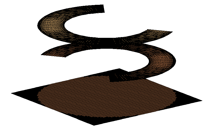
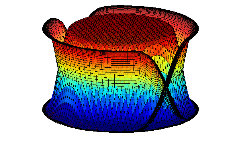
Figure 1: Patches, partition of unity and discretization for a disc. Left: the disc is covered by an interior patch and two edge patches. Right: partition of unity functions $W^{q}_{i}$ supported on the patches. Notice the quadratic refinement along the edges.

4.2 Partition of unity and Nyström nodes

The integration rules mentioned in point 2 in Section 4.1 rely on a decomposition of a given open surface (screen) $\Gamma$ as a union

$$\left(\bigcup_{q=1}^{Q_{1}}\mathcal{P}_{1}^{q}\right)\bigcup\left(\bigcup_{q=1}^{Q_{2}}\mathcal{P}_{2}^{q}\right)$$ (19)

of overlapping patches, including interior patches $\mathcal{P}_{1}^{q}$, $q=1,\dots,Q_{1}$, and edge patches $\mathcal{P}_{2}^{q}$, $q=1,\dots,Q_{2}$. For each $q$, the interior patch $\mathcal{P}_{1}^{q}$ (resp. edge patch $\mathcal{P}_{2}^{q}$) is assumed to be parametrized by an invertible smooth mapping $\mathbf{r}_{1}^{q}=\mathbf{r}_{1}^{q}(u,v)$, $\mathbf{r}_{1}^{q}:\quad\mathcal{H}_{1}^{q}\rightarrow\mathcal{P}_{1}^{q}$ (resp. $\mathbf{r}_{2}^{q}=\mathbf{r}_{2}^{q}(u,v)$, $\mathbf{r}_{2}^{q}:\quad\mathcal{H}_{2}^{q}\rightarrow\mathcal{P}_{2}^{q}$) defined over an open domain $\mathcal{H}_{1}^{q}\subset\mathbb{R}^{2}$ (resp. $\mathcal{H}_{2}^{q}\subset\mathbb{R}^{2}\bigcap\{v\geq 0\}$). Note that, for the $q$-th edge patch, the restriction of the mapping $\mathbf{r}_{2}^{q}$ to the set $\mathcal{H}_{2}^{q}\cap\{v=0\}$ (which we assume is non-empty for $q=1,\dots,Q_{2}$) provides a parametrization of a portion of the edge of $\Gamma$; see Figure (1). Following [9], further, we introduce a partition of unity (POU) subordinated to the set of overlapping patches mentioned above. In detail, the POU we use is a set of non-negative functions $W_{1}^{q}$ and $W_{2}^{q}$ defined on $\Gamma$, $q=1,\dots,Q_{1}$ and $q=1,\dots,Q_{2}$, such that, for all $q$, $W_{1}^{q}$ vanishes outside $\mathcal{P}_{1}^{q}$, $W_{2}^{q}$ vanishes outside $\mathcal{P}_{2}^{q}$, and the relation

$$\sum_{q=1}^{Q_{1}}W_{1}^{q}+\sum_{q=1}^{Q_{2}}W_{2}^{q}=1$$

holds throughout $\Gamma$. The POU can be used to decompose the integral of any function over the surface into a patch-wise sum of the form

$$\begin{split}\int_{\Gamma}f(\mathbf{r}^{\prime})dS^{\prime}=\sum\limits_{j=1}^{2}\sum\limits_{q=1}^{Q_{j}}\int_{\mathcal{H}_{j}^{q}}f\left(\mathbf{r}^{q}_{j}(u,v)\right)W_{j}^{q}\left(\mathbf{r}^{q}_{j}(u,v)\right)J^{q}_{j}(u,v)dudv,\end{split}$$ (20)

where $J^{q}_{j}(u,v)$ denote the Jacobian associated with the parametrization $\mathbf{r}_{j}^{q}$. At this stage we define the set of Nyström nodes: introducing, for each $q$, a tensor-product mesh $\{(u^{q,j}_{\ell},v^{q,j}_{m})\}$ within $\mathcal{H}_{j}^{q}$ (for $j=1$, $2$), we obtain points $\mathbf{r}^{q,j}_{l,m}=\mathbf{r}_{j}^{q}(u^{q,j}_{\ell},v^{q,j}_{m})$ on the surface $\Gamma$. For every $j=1,2$ and every $q=1,\dots,Q_{j}$, the set of nodes $\mathbf{r}^{q,j}_{l,m}$ for which the POU function $W_{j}^{q}$ associated with the patch $\mathcal{P}_{j}^{q}$ does not vanish

$$\mathcal{N}^{q,j}=\left\{\mathbf{r}^{q,j}_{l,m}\,:\,W^{q}_{j}(\mathbf{r}^{q,j}_{l,m})>0\right\}$$ (21)

defines the set of Nyström nodes on the the patch $\mathcal{P}_{j}^{q}$. The overall set $\mathcal{N}$ of Nyström nodes on the surface $\Gamma$ mentioned in Section 4.1, is given by

$$\mathcal{N}=\bigcup_{j=1}^{2}\bigcup_{q=1}^{Q_{j}}\mathcal{N}^{q,j}.$$ (22)

Remark 1.

For later reference we introduce the classes of functions

$$\mathcal{D}_{1}^{q}=\left\{\phi_{1}^{q}\in C^{\infty}\left(\mathcal{H}^{q}_{1}\right)\;:\;\mathrm{supp}(\phi_{1}^{q})\Subset\mathcal{H}^{q}_{1}\right\}\;,\;q=1,\dots,Q_{1}\;,$$ (23)

$$\mathcal{D}_{2}^{q}=\left\{\phi_{2}^{q}\in C^{\infty}\left(\mathcal{H}^{q}_{2}\right)\;:\;\mathrm{supp}(\phi_{2}^{q})\Subset\mathcal{H}^{q}_{2}\right\}\;,\;q=1,\dots,Q_{2}\;,$$ (24)

where $C^{\infty}\left(\mathcal{H}^{q}_{1}\right)$ denotes the set of infinitely differentiable functions defined on the open set $\mathcal{H}^{q}_{1}$, $C^{\infty}\left(\mathcal{H}^{q}_{2}\right)$ denotes the set of functions defined on the set $\mathcal{H}^{q}_{2}$ that are infinitely smooth on $\mathcal{H}^{q}_{2}$ up to and including the edge $\mathcal{H}^{q}_{2}\cap\{v=0\}$, and where, for sets $A$ and $B\subseteq\mathbb{R}^{n}$ the notation $A\Subset B$ indicates that the closure of $A$ in $\mathbb{R}^{n}$ is a compact subset of $\mathbb{R}^{n}$ that is contained in $B$.

4.3 Canonical decomposition and high-order quadrature rules

The high-order numerical quadratures required by step 2. in Section 4.1 are obtained by applying the patch-wise decomposition (20) to the weighted integral operators $\mathbf{S}_{\omega}$ and $\mathbf{N}_{\omega}$ and reducing each one of them to a sum of patch-integrals which, as shown in Sections 5 through 7, can be classified into six distinct canonical types. For each of these canonical types we construct, in Sections 8 and 9, spectrally convergent quadrature rules on the basis of the Nyström points $\mathcal{N}^{q,j}$. Suggestions concerning selection of sizes of the edge and interior patches, which are dictated on the basis of efficiency and accuracy considerations, are put forth in Section 10.

4.4 Computational implementation and efficiency

The high-order methods presented in the following sections enable accurate and fast computation of each one of the six canonical integral types mentioned in Section 4.3. For added efficiency, however, our solver exploits common elements that exist between the various canonical integration algorithms, to avoid re-computation of quantities such as the trigonometric functions associated with the Green’s function, partition of unity functions, integral weights, etc. Additional efficiency could be gained by incorporating an acceleration method (see e.g. [9] and references therein) and code parallelization.

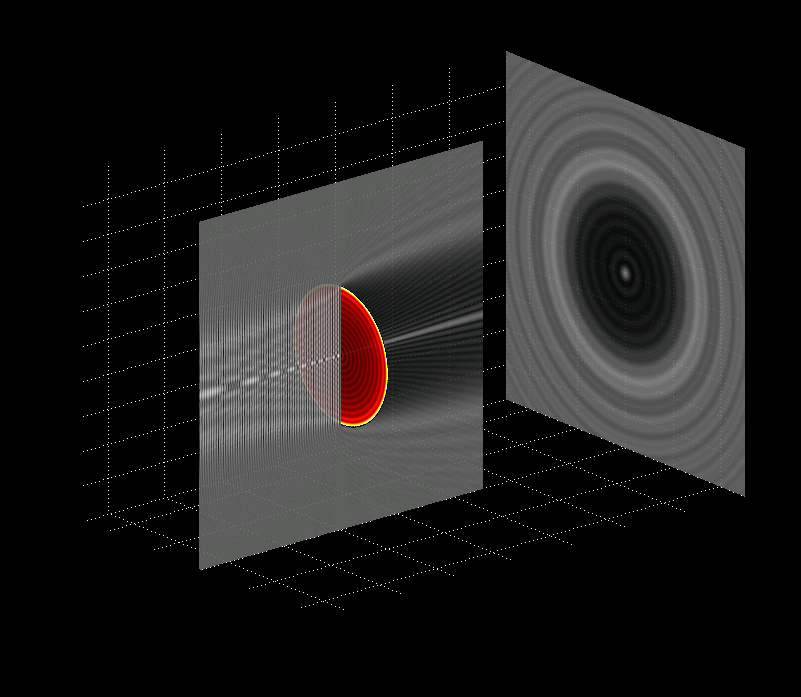
Figure 2: Diffraction by an infinitely thin disc: solution to the Neumann problem for a disc of diameter $24\lambda$ under normal incidence. The famous Poisson spot is clearly visible at the center of the shadow area; see also Figure 12. The coloring on the disc represents the values of the surface unknown $\psi$.

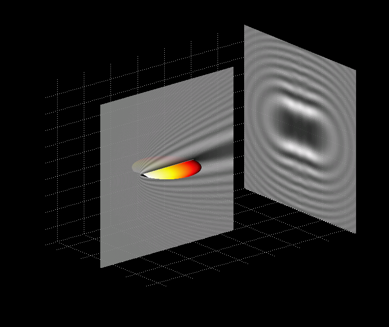
Figure 3: Diffraction by an infinitely thin disc: solution to the Dirichlet problem for a disc of diameter $24\lambda$ under incidence parallel to the disc. The coloring on the disc represents the values of the surface unknown $\phi$.

5 Canonical singular-integral decomposition of the operator $\mathbf{S}_{\omega}$

In view of equation (20), we express the weighted single-layer operator $\mathbf{S}_{\omega}$,

$$\mathbf{S}_{\omega}[\varphi](\mathbf{r})=\int_{\Gamma}G_{k}(\mathbf{r},\mathbf{r}^{\prime})\frac{\varphi(\mathbf{r}^{\prime})}{\omega(\mathbf{r}^{\prime})}dS^{\prime},$$ (25)

in the form

$$\mathbf{S}_{\omega}=\sum\limits_{q=1}^{Q_{1}}\mathcal{S}_{1}^{q}+\sum\limits_{q=1}^{Q_{2}}\mathcal{S}_{2}^{q},$$ (26)

where

$$\mathcal{S}^{q}_{j}[\varphi](\mathbf{r})=\int_{\mathcal{H}_{j}^{q}}G_{k}(\mathbf{r}_{j}^{q}(u,v),\mathbf{r})\frac{\varphi\left(\mathbf{r}^{q}_{j}(u,v)\right)}{\omega\left(\mathbf{r}^{q}_{j}(u,v)\right)}J^{q}_{j}(u,v)W^{q}_{j}(\mathbf{r}^{q}_{j}(u,v))dudv,\quad j=1,2.$$ (27)

In Sections 5.1 and 5.2 the integrals (27) are expressed in terms of canonical integrals of various types.

5.1 Interior patch decomposition

For an interior patch $\mathcal{P}^{q}_{1}$ and for a point $\mathbf{r}\in\Gamma\setminus\mathcal{P}^{q}_{1}$, the integrand in (27) is smooth and compactly supported within the domain of integration $\mathcal{H}^{q}_{1}$—since the weight $\omega(\mathbf{r})$ is smooth and nonzero away from the edge, and since the POU function $W^{q}_{1}$ vanishes outside $\mathcal{H}^{q}_{1}$—and, thus, the integral (27) gives rise to our first canonical integral type:

$$\begin{split}&\mbox{Canonical Integral of Type I}\\ \mathcal{I}^{q,reg}_{1}[\phi_{1}]=\int_{\mathcal{H}_{1}^{q}}\phi_{1}&(u,v)dudv\quad,\quad\phi_{1}\in\mathcal{D}_{1}^{q}\;,\end{split}$$ (28)

see Remark 1. For a point $\mathbf{r}\in\mathcal{P}^{q}_{1}$, $\mathbf{r}=\mathbf{r}^{q}_{1}(u_{0},v_{0})$ for some $(u_{0},v_{0})\in\mathcal{H}^{q}_{1}$, on the other hand, the integrand of (27) with $j=1$ has an integrable singularity at the point $(u_{0},v_{0})$ (cf. equation (4)). Following [9] we express the kernel as a sum of a localized singular part, and a smooth remainder, $G_{k}=G_{k}^{sing}+G_{k}^{reg}$, where

$$G_{k}^{sing}=\eta_{\mathbf{r}}G_{k}^{re},\quad G_{k}^{reg}=(1-\eta_{\mathbf{r}})G_{k}^{re}+iG_{k}^{im}.$$ (29)

Here, $G_{k}^{\textit{re}}(\mathbf{r},\mathbf{r}^{\prime})=\frac{\cos(k|\mathbf{r}-\mathbf{r}^{\prime}|)}{|\mathbf{r}-\mathbf{r}^{\prime}|}$ and $G_{k}^{im}(\mathbf{r},\mathbf{r}^{\prime})=\frac{\sin(k|\mathbf{r}-\mathbf{r}^{\prime}|)}{|\mathbf{r}-\mathbf{r}^{\prime}|}$ denote the real and imaginary parts of the kernel $G_{k}(\mathbf{r},\mathbf{r}^{\prime})$, respectively, and $\eta_{\mathbf{r}}$ is a smooth function which vanishes outside a neighborhood of the point $\mathbf{r}$. As in the previous reference, the collection of all pairs $(\eta_{\mathbf{r}},1-\eta_{\mathbf{r}})$ for $\mathbf{r}\in\Gamma$ is called a floating partition of unity. The integral that arises as $G_{k}$ is replaced in (27) by $G_{k}^{reg}$, has a smooth integrand which is compactly supported within $\mathcal{H}_{1}^{q}$; clearly, this is an integral of canonical type I. The integral obtained by substituting $G_{k}$ by $G^{sing}_{k}$, on the other hand, gives rise to our second canonical type

$$\begin{split}&\mbox{Canonical Integral of Type II}\\ \mathcal{I}^{q,sing}_{1}[\phi_{1}](u_{0},v_{0})=\int_{\mathcal{H}_{1}^{q}}&\frac{\phi_{1}(u,v)}{|\mathbf{R}|}dudv,\quad\phi_{1}\in\mathcal{D}_{1}^{q}\end{split}$$ (30)

where for the sake of conciseness, we have set $\mathbf{R}=\mathbf{r}^{q}_{1}(u_{0},v_{0})-\mathbf{r}_{1}^{q}(u,v)$ and where the point $(u_{0},v_{0})$ belongs to $\mathcal{H}^{q}_{1}$.

5.2 Edge-patch decomposition 

The edge singularity on an edge patch $\mathcal{P}^{q}_{2}$ is characterized in terms of the asymptotic form (12). In what follows we assume, as we may, that on each edge patch,the weight $\omega$ is given by an expression of the form

$$\omega(\mathbf{r}^{q}_{2}(u,v))=\omega_{2}^{q}(u,v)\sqrt{v},$$ (31)

where the function $\omega_{2}^{q}(u,v)$ is smooth up to the edge and it does not vanish anywhere along the edge. It follows that for an edge patch $\mathcal{P}^{q}_{2}$ and for a point $\mathbf{r}\in\Gamma\setminus\mathcal{P}^{q}_{2}$, the operator $\mathcal{S}_{2}^{q}$ defined in equation (27) for $j=2$ takes the form of an integral of our third canonical type:

$$\begin{split}&\mbox{Canonical Integral of Type III}\\ \mathcal{I}^{q,reg}_{2}[\phi_{2}](u_{0},v_{0})=\int_{\mathcal{H}_{2}^{q}}&\phi_{2}(u,v)\frac{dudv}{\sqrt{v}},\quad\phi_{2}\in\mathcal{D}^{q}_{2}.\end{split}$$ (32)

Finally, for an edge patch $\mathcal{P}^{q}_{2}$ and for a point $\mathbf{r}\in\mathcal{P}^{q}_{2}$ we once again use the floating partition of unity to decompose the Green function as a sum of a singular and a regular term. The regular term results in a canonical integral of Type III, and the singular term gives rise to our fourth canonical type:

$$\begin{split}&\mbox{Canonical Integral of Type IV}\\ \mathcal{I}^{q,sing}_{2}[\phi_{2}]=\int_{\mathcal{H}_{2}^{q}}&\frac{\phi_{2}(u,v)}{|\mathbf{R}|}\frac{dudv}{\sqrt{v}},\quad\phi_{2}\in\mathcal{D}_{2}^{q}\end{split}$$ (33)

where $\mathbf{R}=\mathbf{r}^{q}_{2}(u_{0},v_{0})-\mathbf{r}^{q}_{2}(u,v)$.

6 Canonical decomposition of the operator $\mathbf{N}_{\omega}$

In view of equations (6) and (13) the operator $\mathbf{N}_{\omega}$ is given by the point-wise limit

$$\mathbf{N}_{\omega}[\psi](\mathbf{r})\equiv\lim\limits_{z\rightarrow 0}\frac{\partial}{\partial\textbf{n}_{\mathbf{r}}}\int_{\Gamma}\frac{\partial G_{k}(\mathbf{r},\mathbf{r}^{\prime}+z\textbf{n}_{\mathbf{r}^{\prime}})}{\partial\textbf{n}_{\mathbf{r}}^{\prime}}\psi(\mathbf{r}^{\prime})\omega(\mathbf{r}^{\prime})dS^{\prime},\textbf{ }\quad\mathbf{r}\in\Gamma.$$ (34)

Following the open-arc derivation [15, 19, 12] we obtain an adequate expression for this “hypersingular operator” by taking advantage of the following lemma.

Lemma 1.

The operator $\mathbf{N}_{\omega}$ can be expressed in the form

$$\mathbf{N}_{\omega}=\mathbf{N}_{\omega}^{g}+\mathbf{N}_{\omega}^{pv}\mathcal{T}_{\omega}$$ (35)

where, denoting the surface gradient with respect to $\mathbf{r}^{\prime}$ by $\nabla^{s}_{\mathbf{r}^{\prime}}$ and letting $[\,\cdot\,,\cdot\,]$ denote the vector product, the operators $\mathbf{N}_{\omega}^{g}$, $\mathbf{N}_{\omega}^{pv}$ and $\mathcal{T}_{\omega}$ are given by

$$\mathbf{N}_{\omega}^{g}[\psi](\mathbf{r})=k^{2}\int_{\Gamma}G_{k}(\mathbf{r},\mathbf{r}^{\prime})\psi(\mathbf{r}^{\prime})\omega(\mathbf{r}^{\prime})\textbf{n}_{\mathbf{r}^{\prime}}.\textbf{n}_{\mathbf{r}}dS^{\prime},$$ (36)

$$\mathcal{T}_{\omega}[\psi](\mathbf{r}^{\prime})=\omega^{2}(\mathbf{r}^{\prime})\nabla^{s}_{\mathbf{r}^{\prime}}[\psi](\mathbf{r}^{\prime})+\frac{\psi(\mathbf{r}^{\prime})}{2}\nabla^{s}_{\mathbf{r}^{\prime}}[\omega^{2}](\mathbf{r}^{\prime}),\quad\mbox{and}$$ (37)

$$\mathbf{N}_{\omega}^{pv}[\mathbf{T}](\mathbf{r})=p.v.\int_{\Gamma}\big{[}\nabla_{\mathbf{r}}G_{k}(\mathbf{r},\mathbf{r}^{\prime}),\left[\textbf{n}_{\mathbf{r}^{\prime}},\mathbf{T}(\mathbf{r}^{\prime})\right]\big{]}\cdot\textbf{n}_{\mathbf{r}}\frac{dS^{\prime}}{\omega(\mathbf{r}^{\prime})}.$$ (38)

Proof.

See Appendix A. ∎

As shown in Sections 6.1 through 6.3, we may evaluate $\mathbf{N}_{\omega}$ by relying on Lemma 1 and using quadratures for various types of canonical integrals.

6.1 Canonical decomposition of the operator $\mathbf{N}^{g}_{\omega}$ (equation (36))

Calling $\psi_{2}=\psi\omega^{2}$ we re-express (36) in the form

$$\mathbf{N}_{\omega}^{g}[\psi](\mathbf{r})=k^{2}\int_{\Gamma}G_{k}(\mathbf{r},\mathbf{r}^{\prime})\frac{\left(\psi_{2}(\mathbf{r}^{\prime})\textbf{n}_{\mathbf{r}^{\prime}}.\textbf{n}_{\mathbf{r}}\right)}{\omega(\mathbf{r}^{\prime})}dS^{\prime}.$$ (39)

Since $\omega^{2}(\mathbf{r})$ is a smooth function of $\mathbf{r}$ throughout $\Gamma$, a construction similar to the one used for (25) yields a decomposition of the operator $\mathbf{N}_{\omega}^{s}$ in terms of canonical integrals of types I-IV; see Section 5.

6.2 Canonical decomposition of the operator $\mathcal{T}_{\omega}$ (equation (37))

Making use once again of the POU introduced in Section 4.2, we obtain the decomposition

$$\nabla^{s}_{\mathbf{r}}[\psi](\mathbf{r})=\sum_{q=1}^{Q_{1}}\nabla^{s}_{\mathbf{r}}[\psi W_{1}^{q}](\mathbf{r})+\sum_{q=1}^{Q_{2}}\nabla^{s}_{\mathbf{r}}[\psi W_{2}^{q}](\mathbf{r}),$$

of the surface gradient. The evaluation of the $q$-th term in each one of these sums requires the calculation of partial derivatives of the form

$$\frac{\partial\phi_{1}(u,v)}{\partial u}\quad,\quad\frac{\partial\phi_{1}(u,v)}{\partial v}\;,$$ (40)

$$\frac{\partial\phi_{2}(u,v)}{\partial u}\quad\mbox{and}\quad\frac{\partial\phi_{2}(u,v)}{\partial v}$$ (41)

for functions $\phi_{1}\in\mathcal{D}_{1}^{q}$ and $\phi_{2}\in\mathcal{D}_{2}^{q}$. These partial derivatives can be evaluated efficiently and with high-order accuracy by means of the differentiation methods introduced in Sections 8 and 9 below. In view of equation (37), use of such high-order rules enables high-order evaluation of the operator $\mathcal{T}_{\omega}[\psi](\mathbf{r})$.

6.3 Canonical decomposition of the operator $\mathbf{N}^{pv}_{\omega}$ (equation (38))

It is easy to check that, for a smooth field $\mathbf{T}$, $\mathbf{N}^{pv}_{\omega}[\mathbf{T}]$ can be evaluated as a linear combination of functions of the form $\mathbf{D}^{\mathbf{V}_{\ell}}_{\omega}[\phi_{\ell}]$, where $\mathbf{V}_{\ell}$ is a vector quantity that varies with $\mathbf{r}$ but is independent of $\mathbf{r}^{\prime}$, where the operator $\mathbf{D}^{\mathbf{V}}_{\omega}$ is defined by

$$\mathbf{D}^{\mathbf{V}}_{\omega}[\psi](\mathbf{r})=\mbox{p.v.}\int_{\Gamma}\left\{\nabla_{\mathbf{r}}G_{k}(\mathbf{r},\mathbf{r}^{\prime})\cdot\mathbf{V}\right\}\frac{\psi(\mathbf{r}^{\prime})}{\omega(\mathbf{r}^{\prime})}dS^{\prime},$$ (42)

and where $\phi_{\ell}$ are smooth functions. Applying the decomposition (20) to the operator defined in equation (42) yields

$$\mathbf{D}^{\mathbf{V}}_{\omega}[\psi]=\sum\limits_{q=1}^{Q_{1}}\mathbf{D}_{1}^{\mathbf{V},q}[\psi](\mathbf{r})+\sum\limits_{q=1}^{Q_{2}}\mathbf{D}_{2}^{\mathbf{V},q}[\psi](\mathbf{r}),$$ (43)

where

$$\mathbf{D}_{j}^{\mathbf{V},q}[\psi](\mathbf{r})=\mbox{p.v.}\int_{\mathcal{H}^{q}_{j}}\left\{\nabla_{\mathbf{r}}G_{k}(\mathbf{r},\mathbf{r}^{q}_{j}(u,v))\cdot\mathbf{V}\right\}\frac{\psi(\mathbf{r}^{q}_{j}(u,v))}{\omega(\mathbf{r}^{q}_{j}(u,v))}W_{j}^{q}(\mathbf{r}^{q}_{j}(u,v))J^{q}_{j}(u,v)dudv.$$ (44)

We can express the operator $\mathbf{D}_{j}^{\mathbf{V},q}$ as the sum of a hypersingular operator and a weakly singular operator whose respective kernels are defined by the split

$$\nabla_{\mathbf{r}}G_{k}(\mathbf{r},\mathbf{r}^{\prime})\cdot\mathbf{V}=G_{k}^{pv}+G_{k}^{ws},\quad{}G_{k}^{pv}=-\frac{(\mathbf{r}-\mathbf{r}^{\prime})\cdot\mathbf{V}}{|\mathbf{r}-\mathbf{r}^{\prime}|^{3}},$$ (45)

where the residual kernel $G_{k}^{\textit{ws}}$ equals a sum of functions which are either smooth or weakly singular with singularity $\frac{1}{|\mathbf{r}-\mathbf{r}^{\prime}|}$. Using the partition-of-unity split embodied in equation (20), the operator with kernel $G_{k}^{\textit{ws}}$ can be expressed in terms of integrals of canonical types I-IV. The hypersingular operator with kernel $G^{pv}_{k}$ on the other hand gives rise to our fifth and sixth canonical types:

$$\begin{split}&\mbox{Canonical Integral of Type V}\\ \mathcal{I}_{1}^{q,pv}[\phi_{1}](u_{0},v_{0})=\mbox{p.v.}\int_{\mathcal{H}_{1}^{q}}&\frac{\mathbf{R}\cdot\mathbf{V}}{|\mathbf{R}|^{3}}\phi_{1}(u,v)dudv.\end{split}$$ (46)

$$\begin{split}&\mbox{Canonical Integral of Type VI}\\ \mathcal{I}_{2}^{q,pv}[\phi_{2}](u_{0},v_{0})=\mbox{p.v.}\int_{\mathcal{H}_{2}^{q}}&\frac{\mathbf{R}\cdot\mathbf{V}}{|\mathbf{R}|^{3}}\phi_{2}(u,v)\frac{dudv}{\sqrt{v}}.\end{split}$$ (47)

7 Canonical decomposition of the composite operator $\mathbf{N}_{\omega}\mathbf{S}_{\omega}$

While the action of the composite operator $\mathbf{N}_{\omega}\mathbf{S}_{\omega}$ on a function $\phi$ can be evaluated by producing first $\psi=\mathbf{S}_{\omega}[\phi]$ and then evaluating $\mathbf{N}_{\omega}[\psi]$, both of which can be obtained by the methods described in the previous sections, we have found it advantageous in practice to proceed differently, on the basis of the expression (35); see Remark 5 for more details. Using the decomposition (35), we first evaluate the term $\mathbf{N}^{g}_{\omega}\mathbf{S}_{\omega}[\phi]$ by means of a direct composition: we compute $\mathbf{S}_{\omega}[\phi]$ and then apply $\mathbf{N}^{g}_{\omega}$ to the result using the decompositions put forth in Sections 5 and 6.1 respectively. To evaluate the second term $\mathbf{N}^{pv}_{\omega}\mathbf{S}_{\omega}[\phi]$, on the other hand, we first evaluate the quantity $\mathcal{T}_{\omega}\mathbf{S}_{\omega}[\phi]$ by expressing the surface gradient of $\mathbf{S}_{\omega}[\phi]$ required by equation (37) as

$$\nabla^{s}_{\mathbf{r}}S_{\omega}[\phi](\mathbf{r})=p.v.\int_{\Gamma}\nabla^{s}_{\mathbf{r}}G_{k}(\mathbf{r},\mathbf{r}^{\prime})\frac{\phi(\mathbf{r}^{\prime})}{\omega(\mathbf{r}^{\prime})}dS^{\prime}=\sum_{\ell=1,2}\mathbf{D}_{\omega}^{\tau_{\ell}(\mathbf{r})}[\phi](\mathbf{r}),$$ (48)

where $\tau_{1}(\mathbf{r})$ and $\tau_{2}(\mathbf{r})$ denote two orthogonal tangent vectors to $\Gamma$ at the point $\mathbf{r}$ which vary smoothly with $\mathbf{r}$; the corresponding surface gradient of $\omega^{2}$ can be obtained by direct differentiation of a closed form expression, if available, or by means of the differentiation methods put forth in this paper. The terms in the sum on the right-hand side of (48) are of the form given in equation (42) with $\mathbf{V}=\tau_{\ell}(\mathbf{r})$ ($\ell=1,2$), and thus can be expressed in terms of the canonical integrals of type I-VI, as outlined in Section 6.3.

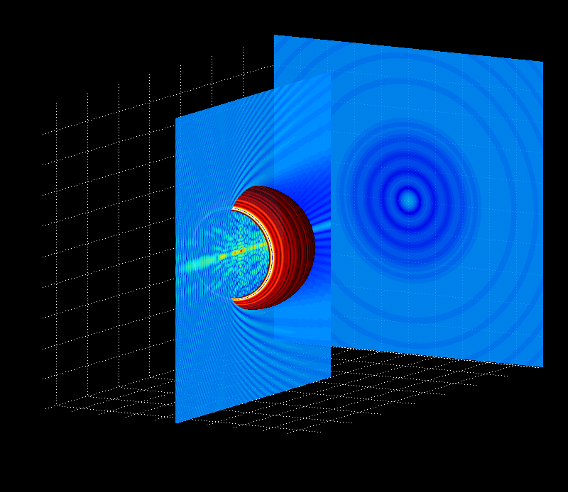
Figure 4: Neumann problem on a spherical cavity of diameter $18\lambda$. The coloring on the spherical wall represents the values of the surface unknown $\psi$.

.

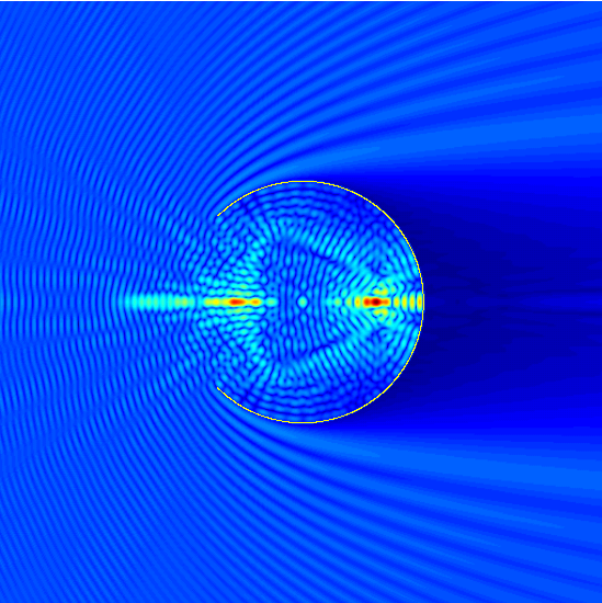
Figure 5: Total Field inside a spherical cavity of diameter $18\lambda$, Dirichlet Problem.

.

8 High-order evaluation of interior-patch operators

In this section we describe our algorithms for evaluation of the interior-patch operators introduced in the previous sections, namely the integral operators of type I, II and V and the differentiation operator (40). To do this, and in accordance with Section 4.2, we assume that the nodes $(u^{q,1}_{\ell},v^{q,1}_{m})$ ($u^{q,1}_{\ell}=u^{q,1}_{0}+\ell h^{q,1}_{u}$, $v^{q,1}_{m}=v^{q,1}_{0}+mh^{q,1}_{v}$, $\ell=1,\dots L^{1}_{q}$, $m=1\dots M^{1}_{q}$), discretize a rectangle that contains $\mathcal{H}^{q}_{1}$.

8.1 Type I Integral (Regular)

We evaluate the canonical Type I integral defined in equation (28) by means of a simple trapezoidal sum over the grid: as noted in [9] the periodicity ($\phi_{1}$ is compactly supported) and smoothness of the integrand gives rise to super-algebraic convergence in this case.

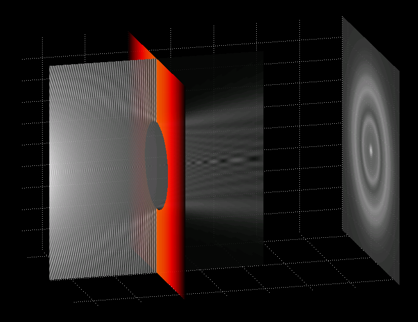
Figure 6: Diffraction by a circular aperture: solution to the Neumann problem for an aperture of diameter $24\lambda$ under point source illumination. The source, which is not visible here, is located to the left of the displayed area. The coloring on the plane is introduced for visual quality, and it does not represent any physical quantity.

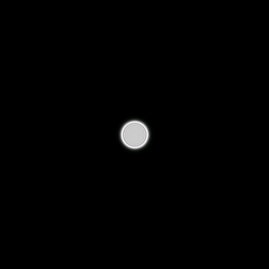
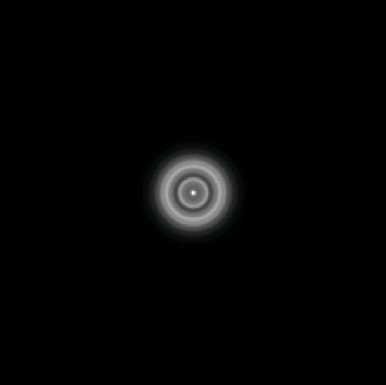
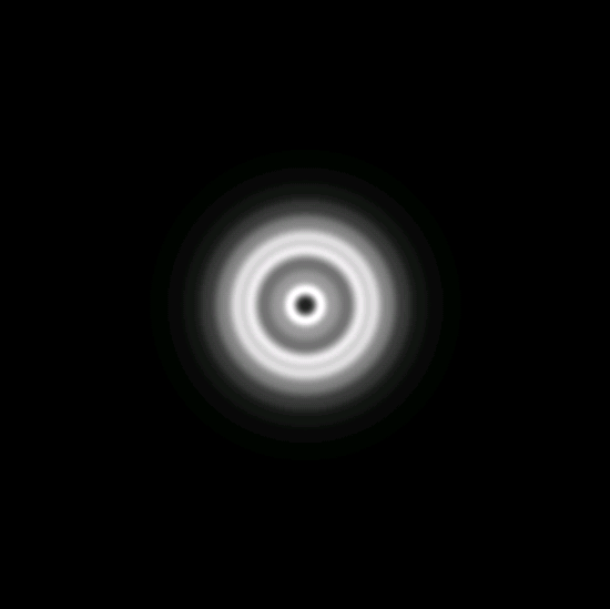
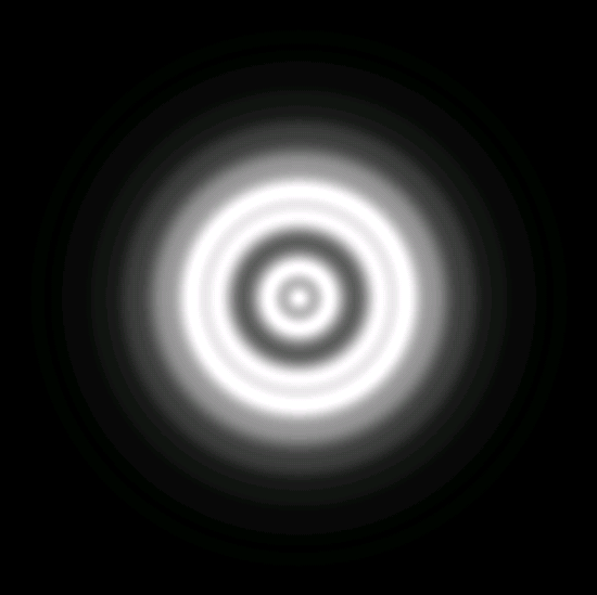
Figure 7: Field diffracted by the circular aperture configuration depicted in Figure 6. From top left to bottom right, depiction of the diffracted field at observation screens located at distances of $6\lambda$, $60\lambda$, $120\lambda$ and $240\lambda$ behind the punctured plane. A dark-spot (the Poisson shadow) can be observed at the center of the illuminated area in the third-to-left image.

.

8.2 Partial Derivatives

In view of the smoothness and periodicity of the function $\phi_{1}$, a standard two-dimensional FFT-based interpolation scheme based on the evenly spaced grid values $\phi^{\ell,m}_{1}$ yields spectrally convergent approximations of the function $\phi_{1}(u,v)$ and its derivatives; our algorithm thus evaluates the derivatives required in equation (40) by performing a direct term by term differentiation of the resulting Fourier representation.

8.3 Type II Integral (Singular)

In order to resolve the singular integrand in equation (30) we utilize the polar change of variables introduced in [9]. Defining $u(\rho,\theta)=u_{0}+\rho\cos\theta$ and $v(\rho,\theta)=v_{0}+\rho\sin\theta$, we obtain

$$\mathcal{I}_{1}^{q,sing}[\phi_{1}](u_{0},v_{0})=\int_{0}^{\pi}I^{q}_{\rho,1}[\phi_{1}](u_{0},v_{0},\theta)d\theta$$ (49)

with

$$I^{q}_{\rho,1}[\phi_{1}](u_{0},v_{0},\theta)=\int_{-\infty}^{\infty}\phi^{\rho}_{1}(\rho,\theta)|\frac{|\rho|}{R}d\rho,$$ (50)

where

$$R=|\mathbf{r}^{q}_{1}(u_{0},v_{0})-\mathbf{r}^{q}_{1}\left(u(\rho,\theta),v(\rho,\theta)\right)|,$$ (51)

and where

$$\phi^{\rho}_{1}(\rho,\theta)=\phi_{1}(u_{0}+\rho\cos\theta,v_{0}+\rho\sin\theta)$$ (52)

is a smooth function of $\rho$ and $\theta$ which vanishes for sufficiently large values of $\rho$. Since, as noted in [9], the ratio $\frac{|\rho|}{R}$ is a smooth function of $\rho$, the integral $I^{q}_{\rho,1}[\phi_{1}](\theta,u_{0},v_{0})$ defined in (50) can be computed accurately via the trapezoidal rule with respect to $\rho$ for any value of $\theta$. Similarly, applying the trapezoidal rule in the $\theta$ variable gives rise to high-order convergence of the integral (49), in view of the $\pi$-periodicity of the integrand.

Remark 2.

Our application of the trapezoidal rule for evaluation of $I_{\rho,1}^{q}(\theta,u_{0},v_{0})$ requires use of equidistant samples in the $\rho$ variable, which for most values of $\theta$, do not correspond to any of the original grid nodes $(u^{q,1}_{\ell},v^{q,1}_{m})$. To address this issue our solver relies on the FFT/cubic-spline interpolation technique presented in [9, Section 3], which allows for fast and efficient evaluation of the required equidistant $\rho$ samples.

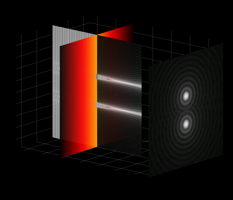
Figure 8: Simulation of Young’s experiment: diffraction by two circular apertures in a sound-hard plane (Neumann boundary conditions); the apertures are 24 wavelengths in diameter. The coloring on the plane, which is introduced for visual quality, does not represent any physical quantity.

8.4 Type V Integral (Principal Value)

An application of the polar change of variables mentioned in Section 8.3 to the principal-value Type V integral (46) results in the expression

$$\mathcal{I}^{q,pv}_{1}[\phi_{1}](u_{0},v_{0})=\int_{0}^{\pi}I^{q,pv}_{\rho,1}[\phi_{1}](u_{0},v_{0},\theta)d\theta,$$ (53)

where $I^{q,pv}_{\rho,1}[\phi_{1}](u_{0},v_{0},\theta)$ is given by the principal value integral

$$I^{q,pv}_{\rho,1}[\phi_{1}](u_{0},v_{0},\theta)=p.v.\int_{-\infty}^{\infty}\frac{|\rho|\mathbf{R}\cdot\mathbf{V}}{R^{3}}\phi^{\rho}_{1}(\rho,\theta)d\rho.$$ (54)

Here the function $\phi^{\rho}_{1}(\rho,\theta)$ is defined by equation (52) and we have set $\mathbf{R}=\mathbf{r}^{q}_{1}(u_{0},v_{0})-\mathbf{r}^{q}_{1}\left(u(\rho,\theta),v(\rho,\theta)\right)$. Equations (53) and (54) form the basis of our algorithm for evaluation of Type V integrals.

Since both $\frac{|\rho|^{3}}{R^{3}}$ and $\frac{\mathbf{R}\cdot\mathbf{V}}{\rho}$ are smooth functions of $\rho$ and $\theta$, it is useful to consider the expression

$$I^{q,pv}_{\rho,1}(u_{0}^{q},v_{0}^{q},\theta)=p.v.\int_{-\infty}^{\infty}\frac{|\rho|^{3}}{R^{3}}\frac{\mathbf{R}\cdot\mathbf{V}}{\rho}\frac{\phi^{\rho}_{1}(\rho,\theta)}{\rho}d\rho,$$ (55)

for the integral (54). This is a 1-dimensional principal value integral of the form

$$I=\mbox{p.v.}\int_{-\infty}^{\infty}\frac{v(x)}{x}dx,$$ (56)

where $v$ is a compactly supported smooth function. Our algorithm proceeds by evaluating this principal value integral by means of a trapezoidal rule algorithm with integration nodes centered symmetrically around $x=0$—which, as shown in [26], yields spectral accuracy for smooth and periodic functions. In detail, letting $x_{i}=({i+\frac{1}{2}})/{M}$, after appropriate scaling into the interval $[-1,1]$, our quadrature for the integral (56) is given by

$$\mbox{p.v.}\int_{-1}^{1}\frac{v(x)}{x}dx\sim\frac{1}{M}\sum_{i=-M}^{M-1}\frac{v(x_{i})}{x_{i}}.$$ (57)

This expression provides spectrally accuracy as long as $v$ is a smooth function of periodicity $2$. Our Type-V integration algorithm is completed by trapezoidal integration in the $\theta$ variable to produce the integral (53) with spectral accuracy.

Remark 3.

Application of the trapezoidal rule (57) to compute the integral (55) requires evenly spaced samples in the $\rho$ variable, which, in addition, must also be symmetrically centered around $\rho=0$. To obtain such samples our algorithm proceeds in two steps: 1) It uses the one-dimensional FFT/spline interpolation method presented in [9, Section 3] to produce evenly spaced samples of the integrand in the $\rho$ variable, and 2) It applies an FFT-based shift (see Remark 4) to produce interpolated samples centered around $\rho=0$. In view of the periodicity and smoothness of the function $v$, this procedure is highly accurate, and it is, in fact significantly faster and less memory intensive than the full two-dimensional spline-table construction presented in [26]—since it only requires storage of one-dimensional tables.

Remark 4.

Given point values $v(x_{i})$ of a smooth and periodic function $v$ on an equispaced grid $x_{i}=x_{0}+ih$, samples of $v$ on a new shifted grid $x_{i}^{*}=x_{i}+\delta$ can be obtained efficiently and with spectral accuracy through use of FFTs. The algorithm proceeds as follows: 1) Evaluation of the FFT of the data set $v(x_{i})$ to produce Fourier coefficients of $v(x)$, 2) Multiplication of each Fourier coefficient by an appropriate exponential, to produce the Fourier coefficients of the shifted function $v(x+\delta)$, and 3) Evaluation of the inverse FFT of the coefficients produced per point 2).

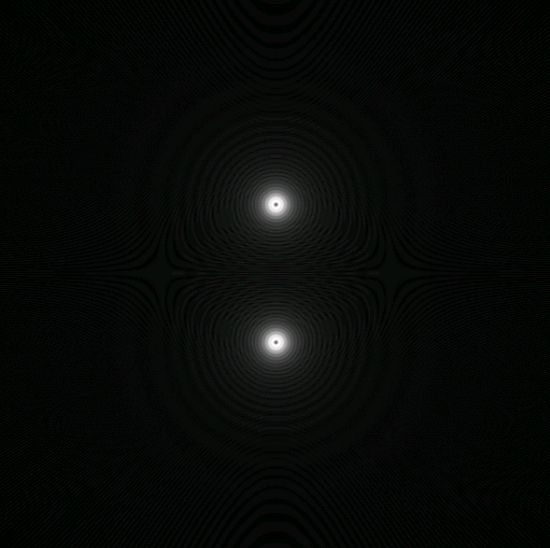
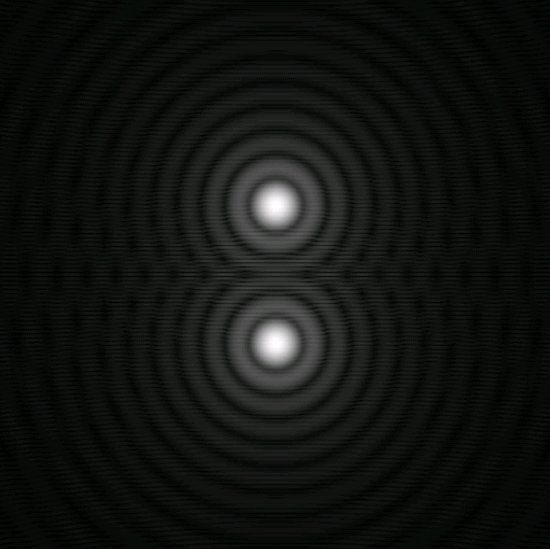
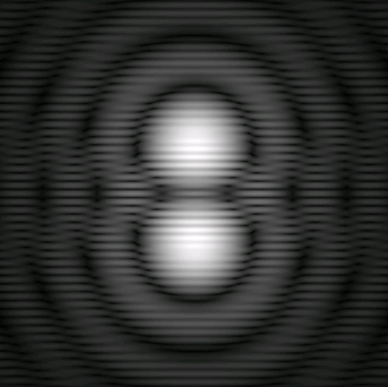
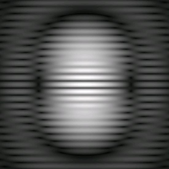
Figure 9: Field diffracted by the two-hole configuration depicted in Figure 8. From left to right, depiction of the diffracted field at observation screens located at distances of $72\lambda$, $576\lambda$, $1728\lambda$ and $3456\lambda$ behind the punctured plane. A dark-spot can be viewed again at the center of the illuminated circles in the left-most image by adequately enlarging the image.

.

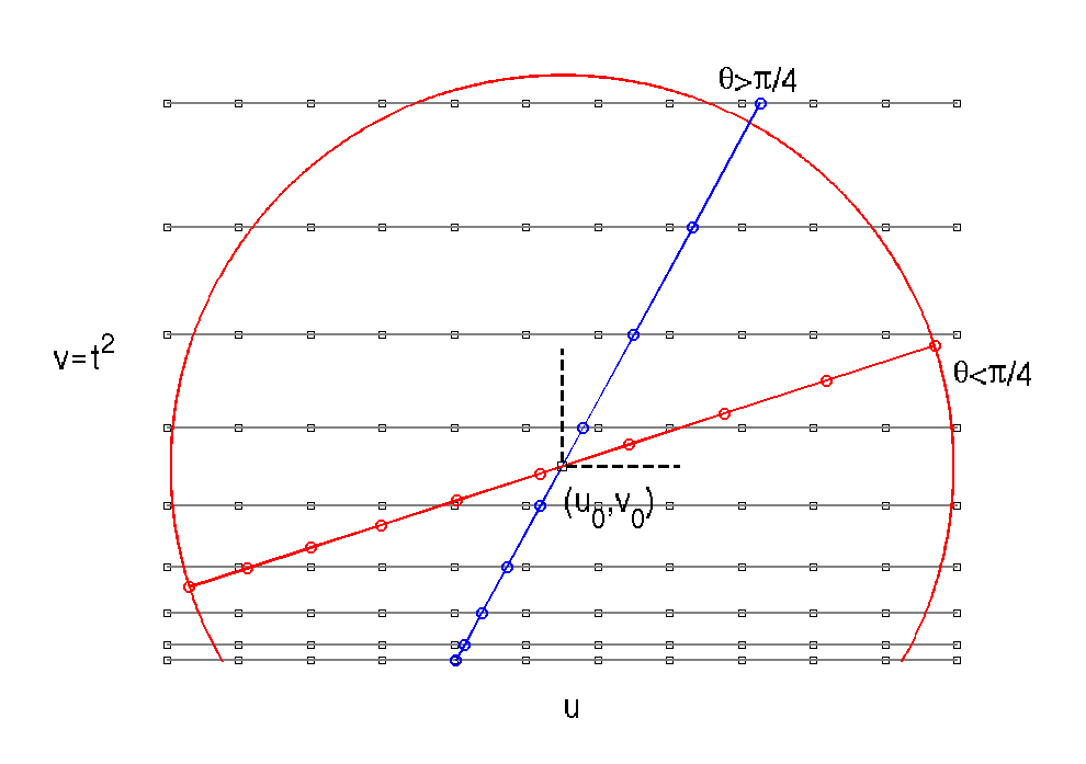
Figure 10: Polar changes of variables around a point close to the edge: quadratic sampling in the $v$ variable, requiring off-grid interpolations for grazing angles.

9 High-order evaluation of edge-patch operators

In this section we describe our algorithms for evaluation of the edge-patch operators, namely the integral operators of type III, IV and VI and the differentiation operator (41). To do this, and in accordance with Section 4.2, we select a tensor product grid $(u^{q,2}_{\ell},v^{q,2}_{m})$ quadratically refined in $v$, which, using spatial mesh-sizes $h^{q,2}_{u}$ and $h^{q,2}_{t}$ in the $u$ and $t$ variables, is given by

$$\left\{\begin{array}[]{cc}u^{q,2}_{\ell}=u^{q,2}_{0}+\ell h^{q,2}_{u},&\ell=1,\dots L^{2}_{q}\\ v^{q,2}_{m}=\left((\frac{1}{2}+m)h^{q,2}_{t}\right)^{2},&m=1\dots M^{2}_{q}.\end{array}\right.$$ (58)

This grid is assumed to discretize a rectangle that contains $\mathcal{H}^{q}_{2}$; in view of the assumptions made on this set (Section 4.2) and the form of the discretization $(u^{q,2}_{\ell},v^{q,2}_{m})$ we see that, while the edge $v=0$ is not itself sampled by this discretization, a parallel line to it, at a distance of $(h^{q,2}_{t}/2)^{2}$ in $(u,v)$ space, is.

9.1 Type III Integral (Regular)

For any smooth function $g$ defined over the interval $[0,1]$ which vanishes identically with all its derivatives at $x=1$, the function $g(t^{2})$ can clearly be extended as a smooth and periodic function of period 2. It follows immediately from the identity

$$\int_{0}^{1}\frac{g(x)}{\sqrt{x}}dx=\int_{-1}^{1}g(t^{2})dt=2\int_{0}^{1}g(t^{2})dt$$ (59)

that the trapezoidal rule approximation

$$\int_{0}^{1}\frac{g(x)}{\sqrt{x}}dx\sim\frac{2}{M}\sum\limits_{m=1}^{M}g\left(t_{m}^{2}\right),\quad t_{m}=\frac{2m+1}{2M},i=0,\dots,M-1$$ (60)

gives rise to super-algebraic convergence. Since the patch discretization $(u^{q,2}_{\ell},v_{m}^{q,2})$ can be expressed in the form $v_{m}^{q,2}=(t_{m}^{q,2})^{2}$, where $t_{m}^{q,2}=(\frac{1}{2}+m)h_{t}^{q,2}$, a two-dimensional trapezoidal rule using this mesh in the set $\mathcal{H}_{2}^{q}$ is super-algebraically convergent.

9.2 Partial Derivatives

In view of the smoothness and periodicity of the function $\phi_{2}(u,t^{2})$, a two-dimensional interpolation scheme based on use of FFTs along the $u$ variable and FCTs (Fast Cosine Transform) along the $t$ variable yields spectrally convergent approximations of the function $\phi_{2}(u,t^{2})$ and its derivatives. Our algorithm thus evaluates the derivatives required in equation (41) by performing a direct term by term differentiation of the resulting Fourier representations together with the expression

$$\frac{\partial\phi_{2}(u,t^{2})}{\partial v}=\frac{1}{2t}\frac{\partial}{\partial t}\left[\phi_{2}(u,t^{2})\right].$$ (61)

Remark 5.

In view of the presence of the $t=\sqrt{v}$ denominator on the right-hand side of equation (61), evaluation of partial derivatives of the function $\phi_{2}(u,v)$ with respect to $v$ on the basis of a term by term differentiation of cosine expansion of the function $\phi_{2}(u,t^{2})$, while yielding spectrally accurate results, is less accurate near the edge than away from the edge—in close analogy with the well-known relative loss of accuracy around end points in Chebyshev-based numerical differentiation. This is why our algorithm was designed to evaluate the composite operator $\mathbf{N}_{\omega}\mathbf{S}_{\omega}$ by first producing the combination $\mathcal{T}_{\omega}\mathbf{S}_{\omega}$ via the rules derived for $D_{\omega}^{\mathbf{T}}$ as explained in Section 7, thus avoiding numerical differentiation. Unfortunately, in the evaluation of the operator $\mathbf{N}_{\omega}$ (which is necessary e.g. for solution of equation equation (15)), direct computation of derivatives and associated accuracy loss does not seem to be avoidable.

9.3 Type IV Integral (Singular)

As in Section 8.3, we utilize a polar change of variables to resolve the Green’s function singularity in the canonical type defined in equation (33), thus obtaining the expression

$$\mathcal{I}_{2}^{q,sing}[\phi_{2}](u_{0},v_{0})=\int_{0}^{\pi}\left(\int_{-\frac{v_{0}}{\sin\theta}}^{\infty}H(u_{0},v_{0},\rho,\theta)\frac{d\rho}{\sqrt{v_{0}+\rho\sin\theta}}\right)d\theta,$$ (62)

where the integrand $H(u_{0},v_{0},\rho,\theta)=\phi_{2}(u_{0}+\rho\cos\theta,v_{0}+\rho\sin\theta)\frac{|\rho|}{R}$ is a smooth function of $\rho$ and $\theta$, which vanishes for $\rho$ larger than a certain constant $\rho_{0}$. While the square-root singularity in the inner-integral can clearly be resolved to high-order by applying an appropriate quadratic change of variable, the outer integrand in $\theta$ is not a uniformly smooth function: as detailed in Appendix B, it develops a boundary-layer as $v_{0}$ approaches $0$. The analysis presented in Appendix B suggests a simple and efficient method for high-order resolution of this boundary layer—thus leading to accurate evaluation of the integral (62). This methodology, which is an integral part of our solver, is described in what follows.

The aforementioned boundary-layer integration method is based on use of the change of variables $t=\sqrt{v_{0}+\rho\sin\theta}$. With this change of variables equation (62) becomes

$$\mathcal{I}_{2}^{q,sing}[\phi_{2}](u_{0},v_{0})=\int_{0}^{\pi}I_{\rho,2}^{q}[\phi_{2}](u_{0},v_{0},\theta)d\theta,$$ (63)

$$I_{\rho,2}^{q}[\phi_{2}](u_{0},v_{0},\theta)=\int_{0}^{\infty}H(u_{0},v_{0},\frac{t^{2}-v_{0}}{\sin\theta},\theta)dt.$$ (64)

The integral (64) is evaluated with high-order accuracy by means of a trapezoidal rule in the $t$ variable, for any $0<\theta<\pi$. In order to capture the boundary-layer in the outer-integral in (63), our algorithm relies on an additional changes of variables $\theta=\alpha^{2}$ and $\theta=\pi-\alpha^{2}$, which lead to the expression

$$\int_{0}^{\pi}I^{q}_{\rho,2}[\phi_{2}](u_{0},v_{0},\theta)d\theta=\int_{0}^{\sqrt{\frac{\pi}{2}}}\left(I^{q}_{\rho,2}[\phi_{2}](u_{0},v_{0},\alpha^{2})-I^{q}_{\rho,2}[\phi_{2}](u_{0},v_{0},\pi-\alpha^{2})\right)\alpha d\alpha.$$ (65)

In view of the analysis presented in Appendix B, the boundary layer is confined to the interval $[0,\alpha^{*}(v_{0})]$, where $\alpha^{*}(v_{0})=(\frac{v_{0}}{d})^{\frac{1}{3}}$, and we therefore decompose the $\alpha$-integral in the form

$$\int_{0}^{\sqrt{\frac{\pi}{2}}}\dots d\alpha=\int_{0}^{\alpha^{*}(v_{0})}\dots d\alpha+\int_{\alpha^{*}(v_{0})}^{\sqrt{\frac{\pi}{2}}}\dots d\alpha.$$ (66)

For a given error tolerance, our algorithm proceeds by applying Chebyshev integration rules to both integrals in (66), using for the second integral a number of integration points that does not depend on $v_{0}$, and using for the first integral a number of integration points that grows slowly as $v_{0}$ tends to zero. In practice, we have found that a mild logarithmic growth in the number of integration points suffices to give consistently accurate results. In view of such slow required growth, and for the sake of simplicity, the number of integration points used for evaluation of the first integral in (66) was taken to be independent of $v_{0}$ and sufficiently large to meet prescribed error tolerances; we estimate that a minimal additional computing time results from this practice in all of the examples considered in this paper.

Remark 6.

In order to apply the trapezoidal rule (60) for evaluation the integral of (64) we distinguish two cases, as illustrated in Figure 10. For $\frac{\pi}{4}\leq\theta\leq\frac{3\pi}{4}$ we use the sampling in $t$ provided by intersections with the original grid underlying $\mathcal{P}^{q}_{2}$: the 1-dimensional cubic-spline interpolation method introduced in section 8.3 can be used to efficiently interpolate the function $H(\frac{t^{2}-v_{0}}{\sin\theta},\theta)$ at the needed integration points. For $0\leq\theta\leq\frac{\pi}{4}$ and $\frac{3\pi}{4}\leq\theta\leq\pi$, on the other hand, the $t$-sampling provided by the intersections with the original grid is too coarse. In this case, we resort to a full two-dimensional interpolation of the density $\phi_{2}$ (see Remark 7) to interpolate to a mesh in the $t$ variable which, away from $t=0$ has roughly the same sampling density as that in the overall patch discretization. In practice a fixed number of discretization points is used to discretize all of the $t$ integrals considered in the present remark.

Remark 7.

The two-dimensional interpolation method for smooth functions $\phi_{2}(u,v)$, which is mentioned in Remark 6, proceeds by first performing a two-dimensional Fourier expansion of the function $\phi_{2}(u,t^{2})$, by means of FFTs along the $u$ variable and FCTs along the $t=\sqrt{v}$ variable, followed zero-padding by a factor $P$ (in practice we use $P=6$). This procedure results in a spectral approximation of $\phi_{2}$ (and, by term-by-term differentiation, of its derivatives as well) on a highly resolved two-dimensional grid. The final interpolation scheme is obtained by building bi-cubic spline interpolations based on function values and derivatives on each square of the refined grid. [22, p. 195].

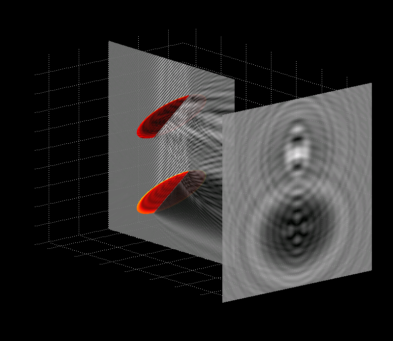
Figure 11: Multiple scattering examples: Neumann problem on two parallel discs $24\lambda$ in diameter, illuminated at a $45$ degree angle. The coloring on the discs represents the values of the surface unknown $\psi$.

9.4 Type VI Integral (Principal Value)

Our algorithm evaluates the principal-value edge-patch Type VI canonical integral $\mathcal{I}^{q,pv}_{2}$ in a manner similar to that used for Type IV treated in Section 9.3: introducing the local polar change of variables around the point $\mathbf{r}$ we obtain

$$\mathcal{I}^{q,pv}_{2}[\phi_{2}](u_{0},v_{0})=\int_{0}^{\pi}\left(p.v.\int_{\frac{-v_{0}}{\sin\theta}}^{\infty}\frac{H^{T}(u_{0},v_{0},\rho,\theta)}{\rho}\frac{d\rho}{\sqrt{v_{0}+\rho\sin\theta}}\right)d\theta,$$ (67)

where

$$H^{T}(u_{0},v_{0},\rho,\theta)=\phi_{2}(u_{0}+\rho\cos\theta,v_{0}+\rho\sin\theta)\frac{|\rho|^{3}}{R^{3}}\frac{\mathbf{R}.\mathbf{T}}{\rho}$$ (68)

is again, a smooth function of $\rho$ and $\theta$ which vanishes identically for $\rho>\rho_{0}$. Resorting to the quadratic change of variables $t=\sqrt{v_{0}+\rho\sin\theta}$ we obtain

$$\mathcal{I}^{q,pv}_{2}[\phi_{2}](u_{0},v_{0})=\int_{0}^{\pi}I^{q,pv}_{\rho,2}[\phi_{2}](u_{0},v_{0},\theta)d\theta.$$ (69)

where the radial integral

$$I^{q,pv}_{\rho,2}[\phi_{2}](u_{0},v_{0},\theta)=p.v.\int_{0}^{\infty}H^{T}(u_{0},v_{0},\frac{t^{2}-t_{0}^{2}}{\sin\theta},\theta)\frac{dt}{t^{2}-t_{0}^{2}},\quad t_{0}=\sqrt{v_{0}}$$ (70)

can be expressed in the form

$$I^{q,pv}_{\rho,2}=\mbox{p.v.}\int_{0}^{\infty}\frac{v(t^{2})}{t^{2}-t_{0}^{2}}dt\quad,\quad\mbox{where $v(t)$ is smooth for $t\geq 0$ and vanishes for $t$ large enough}.$$ (71)

Simple algebra then yields

$$I^{q,pv}_{\rho,2}=\mbox{p.v.}\int_{0}^{\infty}v(t^{2})\left\{\frac{1}{t-t_{0}}-\frac{1}{t+t_{0}}\right\}dt=\mbox{p.v.}\int_{-\infty}^{\infty}\frac{v(t^{2})}{t-t_{0}}dt;$$ (72)

clearly, the right hand side integral in equation (72) can be evaluated with high-order accuracy by means of the trapezoidal rule (57).

Using this algorithm for evaluation of the integral (70) for any fixed value of $\theta$ our algorithm for evaluation of the $\theta$ integral (69), and thus (67), is completed, as in Section 9.3, by relying on (a) The quadratic change of variable $\theta=\alpha^{2}$ and (b) The boundary-layer split (66).

10 Parameter Selection

A number of parameters are implicit in the algorithm laid out in Section 4, including parameters that relate to the overall surface patching and discretization strategies described in Section 4.2 as well as parameters that arise in the polar integration rules introduced in Sections 8.3, 8.4, 9.3 and 9.4. Clearly, the values of such parameters have an impact on both, accuracy for a given discretization density, as well as computing time for a given accuracy tolerance. A degree of experimentation is necessary to produce an adequate selection of such parameters for a given problem. Without entering a full description of the choices inherent in our own implementations, in what follows we provide an indication of the strategies we have used to select two types of parameters, namely, (a) The width of the edge patches (see Figure 1), and (b) The number of discretization points used in both the radial and angular directions for each polar integration problem for which the corresponding floating partition of unity does not vanish at the open edge, as illustrated in Figure 10. Similar (but simpler) considerations apply to other parameters, such as width of floating partitions of unity, extents of overlap between patches, etc.

With respect to point (a) above we note that, for scattering solutions to be obtained with a fixed accuracy tolerance, the discretization densities must be increased as frequencies are increased, and, thus, the width of the edge patches can be decreased accordingly—in such a way that the number of discretization points in the $v$ direction for each one of the edge patches is kept constant. This strategy is crucial for efficiency, since the edge patches require use of the two-dimensional interpolation method mentioned in Remark 7, which is significantly more costly than the corresponding one-dimensional interpolation method used in the interior patches. Use of constant number of $v$-discretization points within shrinking edge patches for increasing frequencies thus enables fixed-accuracy evaluation of edge-patch integrals with an overall computing cost that is not dominated by the edge-patch two-dimensional interpolation procedure.

Concerning point (b) above, in turn, as mentioned in Remark 6, we make use of a fixed number of equispaced integration points in the scaled radial variable $t$ (see equation (63)) for all values of the angular variable $\theta$. In practice, we select the number of $t$-integration points to equal the maximum value $N_{t}$ of the numbers $N_{u}$ and $N_{v}$ of points in the $u$-$v$ discretization mesh that are contained in the $\theta=0$ and $\theta=\pi/2$ lines, respectively, and which lie within the support of the corresponding floating POU. In order to preserve the wavelength sampling in the angular integral (63), finally, the two integrals on the right-hand-side of equation (66) are evaluated on the basis of the Clenshaw-Curtis quadrature rule [22] using an $\alpha$ discretization mesh containing $\frac{\pi}{2}N_{t}$ points—since the length of half a circumference equals $\frac{\pi}{2}$ times its diameter.

11 Numerical Results

In this section, we present results obtained by means of a C++ implementation of the algorithm outlined in Section 4.1, incorporating the canonical operator decompositions introduced in Sections 5 through 7 for the operators $\mathbf{S}_{\omega}$, $\mathbf{N}_{\omega}$ and $\mathbf{N}_{\omega}\mathbf{S}_{\omega}$, together with the high-order integration rules put forth in Sections 8 and 9 and the iterative linear algebra solver GMRES. Errors reported were evaluated through comparisons with highly-resolved numerical solutions. Computation times correspond to single-processor runs (on a 2.67GHz Intel core), without use of the acceleration methods or parallelization. As mentioned in Section 4.4, application of the acceleration method [9] in the present context does not present difficulties; such extension will be considered in forthcoming work.

$N$	Dir($\mathbf{S}_{\omega}$)	Dir($\mathbf{N}_{\omega}\mathbf{S}_{\omega}$)	Neu($\mathbf{N}_{\omega}$)	Neu($\mathbf{N}_{\omega}\mathbf{S}_{\omega}$)
$16\times 16+2\times 24\times 16$	$2.4\times 10^{-4}$	$2.5\times 10^{-4}$	$5.0\times 10^{-4}$	$2.6\times 10^{-4}$
$32\times 32+2\times 48\times 32$	$4.8\times 10^{-6}$	$4.8\times 10^{-6}$	$5.3\times 10^{-6}$	$5.2\times 10^{-6}$
$64\times 64+2\times 98\times 64$	$4.7\times 10^{-8}$	$9.7\times 10^{-8}$	$4.9\times 10^{-8}$	$5.1\times 10^{-8}$

Table 1: Scattering by a disc of diameter $3\lambda$, similar to the corresponding $24\lambda$ simulation depicted in Figure 2. Maximum errors in the acoustic field on the square projection plate shown in the figure. This table demonstrates spectral convergence for all the formulations considered: doubling the discretization density results in orders-of-magnitude decreases in the numerical error. (The notation $Q_{1}\times m_{1}\times n_{1}+Q_{2}\times m_{2}\times n_{2}$ indicates that a number $Q_{1}$ of patches containing $m_{1}\times n_{1}$ discretization points together with a number $Q_{2}$ of patches containing $m_{2}\times n_{2}$ discretization points were used for the corresponding numerical solution.)

		Dir($\mathbf{S}_{\omega}$)			Dir($\mathbf{N}_{\omega}\mathbf{S}_{\omega}$)
Disc Size	Unknowns	It.	Time	$\epsilon_{r}$	It.	Time	$\epsilon_{r}$
$3\lambda$	$4096$	$6$	$58\mbox{s}$	$1.0\times 10^{-4}$	6	$5\mbox{m}20\mbox{s}$	$1.4\times 10^{-4}$
$6\lambda$	$10240$	$9$	$3\mbox{m}5\mbox{s}$	$8.2\times 10^{-5}$	6	$11\mbox{m}14\mbox{s}$	$5.4\times 10^{-5}$
$12\lambda$	$28672$	$13$	$15\mbox{m}21\mbox{s}$	$1.2\times 10^{-4}$	7	$36\mbox{m}31\mbox{s}$	$3.7\times 10^{-4}$
$24\lambda$	$90112$	$18$	$2\mbox{h}30\mbox{m}$	$2.8\times 10^{-4}$	7	$3\mbox{h}41\mbox{m}$	$4.1\times 10^{-4}$
		Neu($\mathbf{N}_{\omega}$)			Neu($\mathbf{N}_{\omega}\mathbf{S}_{\omega}$)
Disc Size	Unknowns	It.	Time	$\epsilon_{r}$	It.	Time	$\epsilon_{r}$
$3\lambda$	$4096$	$16$	$9\mbox{m}21\mbox{s}$	$1.3\times 10^{-4}$	6	$5\mbox{m}50\mbox{s}$	$1.3\times 10^{-4}$
$6\lambda$	$10240$	$28$	$36\mbox{m}31\mbox{s}$	$2.\times 10^{-4}$	6	$11\mbox{m}36\mbox{s}$	$5.8\times 10^{-5}$
$12\lambda$	$28672$	$49$	$2\mbox{h}43\mbox{m}$	$1.7\times 10^{-4}$	7	$37\mbox{m}04\mbox{s}$	$5.2\times 10^{-4}$
$24\lambda$	$90112$	$80$	$21\mbox{h}10\mbox{m}$	$1.9\times 10^{-4}$	7	$3\mbox{h}51\mbox{m}$	$6.1\times 10^{-4}$

Table 2: Iteration numbers and computing times for the problem of scattering by a disc at normal incidence. Top: Dirichlet problem. Bottom: Neumann problem. In each case, use of the second-kind combined operator $\mathbf{N}_{\omega}\mathbf{S}_{\omega}$ gives rise to significantly smaller iteration numbers than the corresponding first kind formulation. In the case of the Neumann problem, the reduction in iteration numbers results in substantially improved computing times. Note: all reported computing times correspond to non-accelerated single-processor runs. Dramatic reductions in computing times would result from use of the acceleration method [9]—see e.g. the recent contribution [8] for the closed-surface case.

11.1 Spectral convergence

We demonstrate the spectral properties of our algorithm through an example concerning a canonical geometry, namely, the unit disc

$$x^{2}+y^{2}\leq 1,\quad z=0.$$ (73)

For this surface we utilize three coordinate patches (see Figure 1), including a large central patch given by equations $\left\{x(u,v)=u,\quad y(u,v)=v,\quad z(u,v)=0\right\}$, and two edge patches parametrized by the equations $\left\{x(u,v)=(1-v)\cos u,\quad y(u,v)=(1-v)\sin u,\quad z(u,v)=0\right\}$ for values of $u$ and $v$ in adequately chosen intervals. The two edge-patches overlap as illustrated in Figure 1, and their width is defined by the range of the $v$ variable, which, in accordance with Section 10, is reduced as the frequency increases. With reference to equation (12), the integral weight is set to $\omega=\sqrt{1-x^{2}-y^{2}}$.

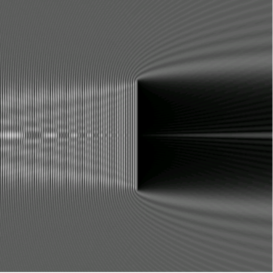
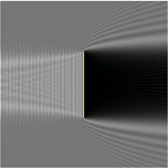
Figure 12: Poisson-spot phenomenon. Left: cross-sectional view on a of the diffraction pattern produced by a disc $24\lambda$ in diameter in three dimensional space (Dirichlet problem, normal incidence). Right: Diffraction by an arc of length $24\lambda$ in two dimensional space (Dirichlet problem, normal incidence). Note that only in the three-dimensional case does a “Poisson cone” and corresponding “Poisson spot” develop in the shadow region.

The sound-soft (Dirichlet) problem can be solved by means of either the first-kind equation (14), or the second-kind equation (16) which, in what follows, are called Dir($\mathbf{S}_{\omega}$) and Dir($\mathbf{N}_{\omega}\mathbf{S}_{\omega}$), respectively. The sound-hard (Neumann) problem, similarly, can be tackled by means of either the first-kind equation (15) or the second-kind equation (17); we call these equations Neu($\mathbf{N}_{\omega}$) and Neu($\mathbf{N}_{\omega}\mathbf{N}_{\omega}$), respectively. Table 1 demonstrates the high-order convergence of the solutions produced by our implementations for each one of these equations on a disc of diameter $3\lambda$; clearly errors decrease by orders of magnitude as a result of a mere doubling of the discretization density.

		Dir$(\mathbf{S}_{\omega})$			Dir$(\mathbf{N}_{\omega}\mathbf{S}_{\omega})$
Spherical Cavity Size	Unknowns	It.	Time	$\epsilon_{r}$	It.	Time	$\epsilon_{r}$
$3\lambda$	$9344$	$17$	$7\mbox{m}16\mbox{s}$	$1.8\times 10^{-4}$	13	$1\mbox{h}18\mbox{m}$	$4.5\times 10^{-4}$
$9\lambda$	$84096$	$39$	$4\mbox{h}06\mbox{m}$	$2.1\times 10^{-4}$	24	$13\mbox{h}20\mbox{m}$	$2.9\times 10^{-4}$
$18\lambda$	$336384$	$65$	$57\mbox{h}48\mbox{m}$	$4.0\times 10^{-4}$	43	$124\mbox{h}$	$1.4\times 10^{-4}$
		Neu$(\mathbf{N}_{\omega})$			Neu$(\mathbf{N}_{\omega}\mathbf{S}_{\omega})$
Spherical Cavity Size	Unknowns	It.	Time	$\epsilon_{r}$	It.	Time	$\epsilon_{r}$
$3\lambda$	$9344$	$57$	1h24m	$1.2\times 10^{-4}$	13	$1\mbox{h}20\mbox{m}$	$8.8\times 10^{-4}$
$9\lambda$	$84096$	$243$	52h14m	$2.\times 10^{-4}$	24	$13\mbox{h}21\mbox{m}$	$5.6\times 10^{-4}$
$18\lambda$	$336384$	$>600$	-	-	43	$124\mbox{h}$	$3.1\times 10^{-4}$

Table 3: Iteration numbers and computing times for the problem of scattering by the spherical cavity defined by equation (74) and depicted in Figures 4 and 5. Top: Dirichlet problem. Bottom: Neumann problem. Reductions in numbers of iterations and computing times occur as detailed in the caption of Table 2, but, owing to the rich multiple scattering phenomena that arise within the cavity, the iteration numbers are significantly higher, in all cavity cases, than those required for the corresponding disc problems.

11.2 Solver performance under various integral formulations

In this section we demonstrate the performance of the open-surface solvers based on use of the operators Dir($\mathbf{S}_{\omega}$) and Dir($\mathbf{N}_{\omega}\mathbf{S}_{\omega}$) for the Dirichlet problem, as well as the operators Neu($\mathbf{N}_{\omega}$) and Neu($\mathbf{N}_{\omega}\mathbf{S}_{\omega}$) for the Neumann problem. We base our demonstrations on two open surfaces: a disc and a spherical cavity defined by

$$x^{2}+y^{2}+z^{2}=1,\quad z>\cos(\theta_{0}),$$ (74)

where $\theta_{0}$ denotes the cavity aperture. For the examples discussed here we set $\theta_{0}=\frac{3\pi}{4}$, and we made use of the weight function $\omega=\sqrt{z-z_{0}}$ where $z_{0}=\cos(\theta_{0})$.

For both geometries, computational times and accuracies at increasingly large frequencies are reported in Tables 2 and 3. In all tables the acronym It. denotes the number of iterations required to achieve a relative error (in a screen placed at some distance from the diffracting surface) equal to “$\epsilon_{r}$” (relative the the maximum field value on the screen), and “Time” denotes the total time required by the solver to evaluate the solution. As can be seen from these tables, the equation Neu($\mathbf{N}_{\omega}$) requires very large number of iterations for the higher frequencies. The computing times required by the low-iteration equation Neu($\mathbf{N}_{\omega}\mathbf{S}_{\omega}$) are thus significantly lower than those required by Neu($\mathbf{N}_{\omega}$). The situation is reversed for the Dirichlet problem: although the equation Dir($\mathbf{N}_{\omega}\mathbf{S}_{\omega}$) requires fewer iterations than Dir($\mathbf{S}_{\omega}$), the total computational cost of the low-iteration equation is significantly higher in this case—since the application of the operator in Dir($\mathbf{S}_{\omega}$), which, fortunately, suffices for the solution of the Dirichlet problem, is substantially less expensive than the application of the operator in Dir($\mathbf{N}_{\omega}\mathbf{S}_{\omega}$). As it happens, at high-frequency, the bulk of the computational time used by our solver is spent on interior-patch work: application of the acceleration method of [9] (see also [8]) would therefore reduce dramatically overall computing times for high-frequency problems.

Figures 2 and 3 display three dimensional renderings of patterns of diffraction by the disc under normal incidence with Neumann boundary condition, and under horizontal incidence with Dirichlet boundary condition. Corresponding images for the spherical-cavity problem are presented in Figures 4 and 5; note the interesting patterns of multiple-scattering and caustics that arise in the cavity interior.

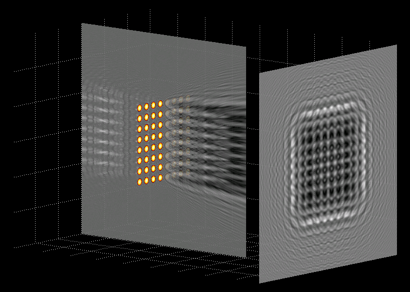
Figure 13: Dirichlet problem on an array of $8\times 8$ discs of diameter $6\lambda$. (Overall diameter: 96.6$\lambda$; 192 patches used.) The coloring on the discs represent the values of the surface unknown $\varphi$.

11.3 Miscellaneous examples

This section presents a variety of results produced by the open-surface solver introduced in this paper, including demonstration of well known effects such as the Poisson spot, and applications in classical contexts such as that provided by the Young experiment.

11.3.1 Poisson spot

As mentioned in the Introduction, the experimental observation of a bright area in the shadow of the disc, the famous Poisson spot, provided one of the earliest confirmations of the wave-theory models of light. The Poisson spot is clearly visible in the diffraction patterns presented in Figure 2 and the left portion of Figure 12. The left portion of Figure 12 displays a slice of the total field around the disc along the $x-z$ plane, which gives a better view of the Poisson-spot phenomenon: the “Poisson cone” is clearly visible in this figure. Interestingly, this phenomenon does not occur in the two-dimensional case. This is demonstrated in the image presented on the right portion of Figure 12: the two-dimensional diffraction pattern arising from the flat unit strip (which was obtained by the solver presented in [10]) gives rise to a dark dark shadow area which does not contain a diffraction spot.

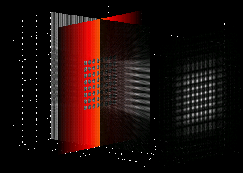
Figure 14: Neumann problem for an array of $8\times 8$ circular apertures of diameter $6\lambda$. The diffracted field depicted in this figure was produced by means of Babinet’s principle from the diffraction pattern displayed in Figure 13. As in Figure 6, the coloring on the plane is introduced for visual quality, and does not represent any physical quantity.

11.4 Babinet’s principle, apertures and Young’s experiment

For a flat open surface $\Gamma$ contained in a plane $\Pi$ one may consider the corresponding problem of diffraction by the complement $\Gamma^{c}=\Pi\setminus\Gamma$ of $\Gamma$ within $\Pi$. As is well known, the diffraction pattern resulting from $\Gamma^{c}$ can be computed easily, by means of the Babinet principle (see Appendix C and, in particular, equation (93)), from a corresponding diffraction pattern associated with the surface $\Gamma$. (For ease of reference, a derivation of the Babinet principle for scalar waves is presented in Appendix C.) In what follows we present three applications of the Babinet principle, namely, the diffraction by a circular aperture, the Young phenomenon, and diffraction across an array of apertures (in Section 11.4.1).

As our first application of Babinet’s principle, in Figure 6 we present the field diffracted by a circular aperture which is $24\lambda$ in diameter. The incident field for this image was taken to be a point source located at the point $(0,0,-10)$, outside the region displayed on the figure. In Figure 7, we display the total field on screens located behind the aperture at varying distance from the punctured plane. Interestingly, under some configurations a dark spot appears in the center of the bright area, in full accordance with Arago’s prediction that a ’Poisson shadow’ must exist. As our second application of Babinet’s principle, in Figure 8 we present the field diffracted by a pair of nearby circular holes in an otherwise perfectly sound-hard plane, under normal plane-wave incidence: this is a setup of the classical Young experiment. This diffraction pattern was produced, by means of Babinet’s principle, from a corresponding solution of a Dirichlet problem for two coplanar discs in space. As in Young’s experiment, interference fringes arise: these can be seen clearly on the right-most image in Figure 9. Again, sharp dark spots at the center of the circular illuminated areas can be seen in the leftmost image in Figure 9.

11.4.1 Arrays of scatterers/apertures

Geometries consisting of a number of disjoint open-surface scattering bodies can be treated easily by the solver introduced in this paper—since the decomposition in patches inherent in equation (19) is not restricted to sets of patches representing a connected surface. The solution for the two-disc diffraction problem presented in the previous section, for example, was obtained in this manner. In what follows we provide a few additional test cases involving composites of open surfaces.

Figure 11 presents the solution of a problem of scattering by two parallel discs illuminated at an angle of $\frac{\pi}{4}$, with Neumann boundary conditions. The beam reflected by the bottom disc, which can clearly be traced onto the upper disc, gives rise to a bright area in the projection screen behind that disc. Two final examples concern an array of 64 discs and the corresponding array of 64 circular apertures on a plane—where each disc is $6\lambda$ in diameter and the discs are separated by $3\lambda$ spacings, for a total array diameter of $96.6\lambda$. The corresponding diffracted fields are presented in Figures 13 and 14. The solution of the Dirichlet problem for the 64 disc array was obtained in $23$ GMRES iterations on a $192$ patch geometry representation.

12 Conclusions

We have introduced a new set of integral equations and associated high-order numerical algorithms for the solution of scalar problems of diffraction by open surfaces. The new open-surface solvers are the first ones in the literature that produce high-order solutions in reduced number of GMRES iterations for general (smooth) open surfaces and arbitrary frequencies. The second-kind formulation Neu($\mathbf{N}_{\omega}\mathbf{S}_{\omega}$) is highly beneficial in the context of the Neumann problem, as it requires computing times that are orders-of-magnitude shorter than those required by the alternative hypersingular formulation N($\mathbf{N}_{\omega}$). Such gains do not occur for the Dirichlet problem: the proposed solver produces high-order solutions to Dir($\mathbf{S}_{\omega}$) in very short computational times, and the gains in iteration numbers that result from use of the formulation Dir($\mathbf{N}_{\omega}\mathbf{S}_{\omega}$) do not suffice to compensate for the significantly higher cost required for evaluation of the operator $\mathbf{N}_{\omega}$. With appropriate parallelization and acceleration, fast and accurate solutions should be achievable by these algorithms for very large structures, thus providing a robust numerical workbench for the solution of classical diffraction problems by open surfaces.

Acknowledgments. The authors gratefully acknowledge support from AFOSR, NSF, JPL and the Betty and Gordon Moore Foundation.

Appendix A Expression of the operator $\mathbf{N}_{\omega}$ in terms of tangential derivatives

In this section, we provide a proof of Lemma 1.

Proof.

It suffices to show that the operators on the left- and right-hand sides of equation (35) coincide when applied to any smooth function $\psi$ defined on $\Gamma$. Following the derivation in [12] for the closed-surface case, we define the weighted double layer operator

$$\mathbf{D}_{\omega}[\psi](\mathbf{r})=\int_{\Gamma}\frac{\partial G_{k}(\mathbf{r},\mathbf{r}^{\prime})}{\partial\mathbf{n}_{\mathbf{r}}^{\prime}}\psi(\mathbf{r}^{\prime})\omega(\mathbf{r}^{\prime})dS^{\prime},$$ (75)

and we evaluate the limit of its gradient as $\mathbf{r}$ tends to $\Gamma$. For $\mathbf{r}$ outside $\Gamma$, (75) can be expressed in the form

$$\mathbf{D}_{\omega}[\psi](\mathbf{r})=-\mbox{div}\int_{\Gamma}G_{k}(\mathbf{r},\mathbf{r}^{\prime})\psi(\mathbf{r}^{\prime})\omega(\mathbf{r}^{\prime})\textbf{n}_{\mathbf{r}^{\prime}}dS^{\prime}.$$ (76)

Thus, using the identity

$$\mbox{curl curl}A=-\Delta A+\nabla\mbox{div }A,$$

we obtain

$$\begin{split}\nabla\mathbf{D}_{\omega}[\psi](\mathbf{r})=k^{2}\int_{\Gamma}G_{k}(\mathbf{r},\mathbf{r}^{\prime})\psi(\mathbf{r}^{\prime})\omega(\mathbf{r}^{\prime})\textbf{n}_{\mathbf{r}^{\prime}}dS^{\prime}\\ -\mbox{curl curl}\int_{\Gamma}G_{k}(\mathbf{r},\mathbf{r}^{\prime})\psi(\mathbf{r}^{\prime})\mathbf{n}_{\mathbf{r}^{\prime}}dS^{\prime}.\end{split}$$ (77)

But, for $\mathbf{r}$ outside $\Gamma$ we have

$$\begin{split}\mbox{curl}\int_{\Gamma}G_{k}(\mathbf{r},\mathbf{r}^{\prime})\psi(\mathbf{r}^{\prime})\textbf{n}_{\mathbf{r}^{\prime}}dS^{\prime}=\\ \int_{\Gamma}\left[\textbf{n}_{\mathbf{r}^{\prime}},\psi(\mathbf{r}^{\prime})\omega(\mathbf{r}^{\prime})\nabla^{s}_{\mathbf{r}^{\prime}}G_{k}(\mathbf{r},\mathbf{r}^{\prime})\right]dS^{\prime},\end{split}$$ (78)

where $[\,\cdot\,,\cdot\,]$ and $\nabla^{s}$ denote the vector product and surface gradient operator, respectively. Integrating by parts the surface gradient (see e.g. [12, eq. (2.2)]) and noting that the boundary terms vanish in view of the presence of the weight $\omega$, we obtain

$$\begin{split}\mbox{curl}\int_{\Gamma}G_{k}(\mathbf{r},\mathbf{r}^{\prime})\psi(\mathbf{r}^{\prime})\textbf{n}_{\mathbf{r}^{\prime}}dS^{\prime}=\\ -\int_{\Gamma}G_{k}(\mathbf{r},\mathbf{r}^{\prime})\left[\textbf{n}_{\mathbf{r}^{\prime}},\nabla^{s}\left(\psi(\mathbf{r}^{\prime})\omega(\mathbf{r}^{\prime})\right)\right]dS^{\prime}.\end{split}$$ (79)

In the limit as $\mathbf{r}$ tends to an interior point in $\Gamma$ we therefore obtain the expression

$$\begin{split}\nabla\mathbf{D}_{\omega}[\psi](\mathbf{r})=k^{2}\int_{\Gamma}G_{k}(\mathbf{r},\mathbf{r}^{\prime})\psi(\mathbf{r}^{\prime})\omega(\mathbf{r}^{\prime})\textbf{n}_{\mathbf{r}^{\prime}}dS^{\prime}\\ +\mbox{p.v.}\int_{\Gamma}\left[\nabla_{\mathbf{r}}G_{k}(\mathbf{r},\mathbf{r}^{\prime}),\left[\textbf{n}_{\mathbf{r}^{\prime}},\nabla^{s}\left(\psi(\mathbf{r}^{\prime})\omega(\mathbf{r}^{\prime})\right)\right]\right]dS^{\prime}\quad\quad(\mathbf{r}\in\Gamma),\end{split}$$ (80)

in terms of a principal value integral, for the surface values of the gradient of the double layer operator $\mathbf{D}_{\omega}$. Taking the scalar product with $\textbf{n}_{\mathbf{r}}$ on both sides of (80) now yields the desired result: equation (35).

∎

Appendix B Boundary-layer character of the inner integral in equation (62)

In order to demonstrate the difficulties inherent in the numerical evaluation of the outer integral in equation (62) we consider the integration problem

$$\int_{0}^{\pi}\tilde{I}_{\rho}(v_{0},\rho_{0},\theta)d\theta,$$ (81)

in which the $(u_{0},v_{0})$-dependent inner integral in (62) is substituted by the $v_{0}$-dependent integral

$$\tilde{I}_{\rho}(v_{0},\rho_{0},\theta)=\int_{-\frac{v_{0}}{\sin\theta}}^{\infty}\tilde{H}_{\rho_{0}}(\rho,\theta)\frac{d\rho}{\sqrt{v_{0}+\rho\sin\theta}}\quad,\quad 0\leq\theta\leq\pi.$$ (82)

Here

$$\tilde{H}_{\rho_{0}}(\rho,\theta)=\left\{\begin{array}[]{ll}1,&|\rho|<\rho_{0}\\ 0,&|\rho|\geq\rho_{0},\end{array}\right.$$ (83)

so that, in the present example, $\rho_{0}$ is the polar-integration radius. (The inner integral in (62) varies smoothly with $u_{0}$, and, thus, the $u_{0}$ dependence does not need to be built into the present analogy.) The integral $\tilde{I}_{\rho}(v_{0},\rho_{0},\theta)$ is given by

$$\tilde{I}_{\rho}(v_{0},\rho_{0},\theta)=\left\{\begin{array}[]{ll}\frac{2\rho_{0}}{\sqrt{v_{0}+\rho_{0}\sin\theta}+\sqrt{v_{0}-\rho_{0}\sin\theta}}&\quad\mbox{if}\quad\sin\theta\leq\frac{v_{0}}{\rho_{0}}\\ &\\ 2\frac{\sqrt{\frac{v_{0}}{\sin\theta}+\rho_{0}}}{\sqrt{\sin\theta}}&\quad\mbox{if}\quad\sin\theta>\frac{v_{0}}{\rho_{0}}.\end{array}\right.$$ (84)

Clearly, as $v_{0}$ tends to zero, $\tilde{I}(v_{0},\rho_{0},\theta)$ becomes increasingly singular (as demonstrated in the left portion of Figure 15): in view of the last equation on the right hand side of (84), we have

$$\lim_{v_{0}\rightarrow 0}\tilde{I}_{\rho}(v_{0},\rho_{0},\theta)=\left(\frac{1}{\sqrt{\sin\theta}}\right).$$ (85)

To treat the singularity in (85) we introduce quadratic changes of variables in the $\theta$ integration in equation (81)—of the form $\theta=\alpha^{2}$ in the interval $[0,\frac{\Pi}{2}]$ and $\theta=\Pi-\alpha^{2}$ in the interval $[\frac{\pi}{2},\pi]$). As a result of these operations we obtain bounded integrands: for example, the integrand resulting from the first of these changes of variables is $\tilde{J}(v_{0},\rho_{0},\alpha)=\alpha\tilde{I}(v_{0},\rho_{0},\alpha^{2})$, which is a bounded function of $\alpha$. This integrand is depicted on the right portion of Figure 15; clearly $\tilde{J}(v_{0},\rho_{0},\alpha)$ develops a boundary layer as $v_{0}$ tends to zero.

The two changes of variables mentioned above result in integrals over the domain $[0,\sqrt{\frac{\pi}{2}}]$), and in both cases boundary layers result at and around $\alpha=0$. To resolve these boundary layers we decompose the integration interval into two sub-intervals, namely $[0,\alpha^{*}(v_{0},\rho_{0})]$ and $[\alpha^{*}(v_{0},\rho_{0}),\sqrt{\frac{\pi}{2}}]$. Here, for a given value of $v_{0}$, the point $\alpha^{*}(v_{0},\rho_{0})$ is chosen to lie to right of the coordinate for which the peak occurs in the right portion of Figure 15, in such a way that the slope of the function $\tilde{J}(v_{0},\rho_{0},\alpha)$ as a function of $\alpha$ at $\alpha=\alpha^{*}(v_{0},\rho_{0})$ remains constant as $v_{0}$ approaches zero—with a slope that equals a certain user-prescribed constant value. In practice we have found that the integral to the right of the point $\alpha=\alpha^{*}(v_{0},\rho_{0})$ can be performed, with fixed accuracy, by means of a number of discretization points that grows very slowly as $v_{0}\to 0$. (In our implementations we typically use a number of discretization points to evaluate this integral that remains constant for all required small values of $v_{0}$.) The evaluation of the integral on the left of the point $\alpha=\alpha^{*}(v_{0},\rho_{0})$ with fixed accuracy requires a number of discretization points that does grow somewhat faster, as $v_{0}\to 0$, than the one on the right, but, we have found in practice that the latter integral can be obtained with fixed accuracy by means of a number of discretization points that grows only logarithmically with $v_{0}$ as $v_{0}\to 0$.

To obtain an approximate expression for $\alpha^{*}(v_{0},\rho_{0})$ we note that, since

$$\tilde{J}(v_{0},\rho_{0},\alpha)=\alpha\frac{\sqrt{v_{0}+\rho_{0}\sin\alpha^{2}}}{\sin\alpha^{2}}\quad\mbox{for}\quad\quad\alpha>\sqrt{\arcsin(\frac{v_{0}}{\rho_{0}})},$$ (86)

for $\alpha\ll 1$ and for sufficiently small values of $v_{0}$ (such that the inequality constraint in (86) is satisfied) we have $\alpha^{2}~{}\sim\sin\alpha^{2}$, and thus letting $\eta=\frac{v_{0}}{\rho_{0}}$,

$$\tilde{J}(v_{0},\rho_{0},\alpha)\sim\sqrt{\rho_{0}}f_{n}(\alpha)\quad\mbox{where}\quad f_{\eta}(\alpha)=\frac{\sqrt{\eta+\alpha^{2}}}{\alpha}.$$ (87)

It follows that, for a given constant $C>0$, the fixed-slope point $\alpha_{\eta}$ for which $f_{\eta}^{\prime}\left(\alpha_{\eta}\right)=-C$ is approximately given as a root of the equation

$$-\frac{\eta}{\alpha_{\eta}^{2}\sqrt{\eta+\alpha_{\eta}^{2}}}=-C,\quad\mbox{or equivalently},\quad\frac{\alpha_{\eta}^{4}}{\eta}+\frac{\alpha_{\eta}^{6}}{\eta^{2}}-\frac{1}{C^{2}}=0.$$ (88)

Clearly, thus, an approximation of the quantity $\alpha_{\eta}^{2}$ can be obtained, in closed form, as a root of a certain polynomial of degree three. A Taylor expansion of the resulting root as a function of $\eta$ around $\eta=0$ shows that

$$\alpha_{\eta}=O\left(\eta^{\frac{1}{3}}\right)\quad\mbox{as}\quad\eta\rightarrow 0,$$ (89)

and, since $\eta=\frac{v_{0}}{\rho_{0}}$, it follows that the constant slope point $\alpha^{*}(v_{0},\rho_{0})$ is given, for each constant $\rho_{0}$, by

$$\alpha^{*}(v_{0},\rho_{0})\sim v_{0}^{\frac{1}{3}}\quad\mbox{as}\quad v_{0}\rightarrow 0.$$ (90)

.

Since the function $H=H(u_{0},v_{0},\rho,\theta)$ in equation (62) is modulated by a smooth windowing function that is akin to the “discontinuous window function” $\tilde{H}_{\rho_{0}}$ in equation (84), it is reasonable to expect that the inner $\rho$-integral in (62) gives rise to a $\alpha$-integrand which develops a similarly behaved, albeit smoother, boundary-layer. We illustrate this in Figure 16 (the left portion of which should be compared to the right portion of Figure 15), which displays the function

$$J(v_{0},\rho_{0},\alpha)=\alpha\int_{-\frac{v_{0}}{\sin\alpha^{2}}}^{\infty}H(v_{0},\rho,\alpha^{2})\frac{\rho_{0}\rho}{\sqrt{v_{0}+\rho_{0}\sin\alpha^{2}}},$$ (91)

where

$$H_{\rho_{0}}(\rho,\theta)=W(\frac{\rho}{\rho_{0}}),\quad W(\rho)=\left\{\begin{array}[]{ll}e^{-\frac{1}{1-\rho^{2}}},&\rho<1\\ 0,&\rho\geq 1.\end{array}\right.$$ (92)

It follows that the $\theta$-integration strategy outlined above in this section for the function $\tilde{I}$ (based on the change of variables $\theta=\alpha^{2}$ and partitioning of integration intervals at the point $\alpha=\alpha^{*}$) applies to the integrand given by the inner integral in equation (62): this strategy is incorporated as part of our algorithm, and is thus demonstrated in the numerical examples presented in Section 11.

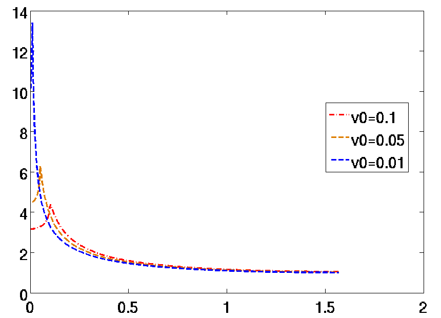
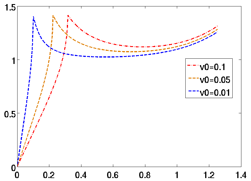
Figure 15: Left: boundary layer for $\tilde{I}(v_{0},\rho_{0},\theta)$ on the interval $[0,\frac{\pi}{2}]$. Right: quadratic regularization $\tilde{J}(v_{0},\rho_{0},\alpha)=\alpha\tilde{I}(v_{0},\rho_{0},\alpha^{2})$, where $\alpha\in[0,\sqrt{\frac{\pi}{2}}]$.

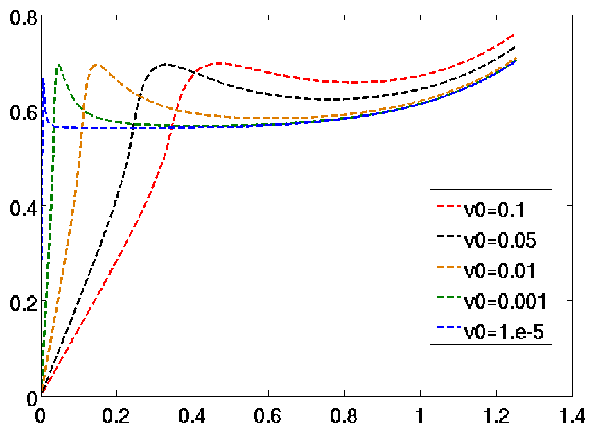
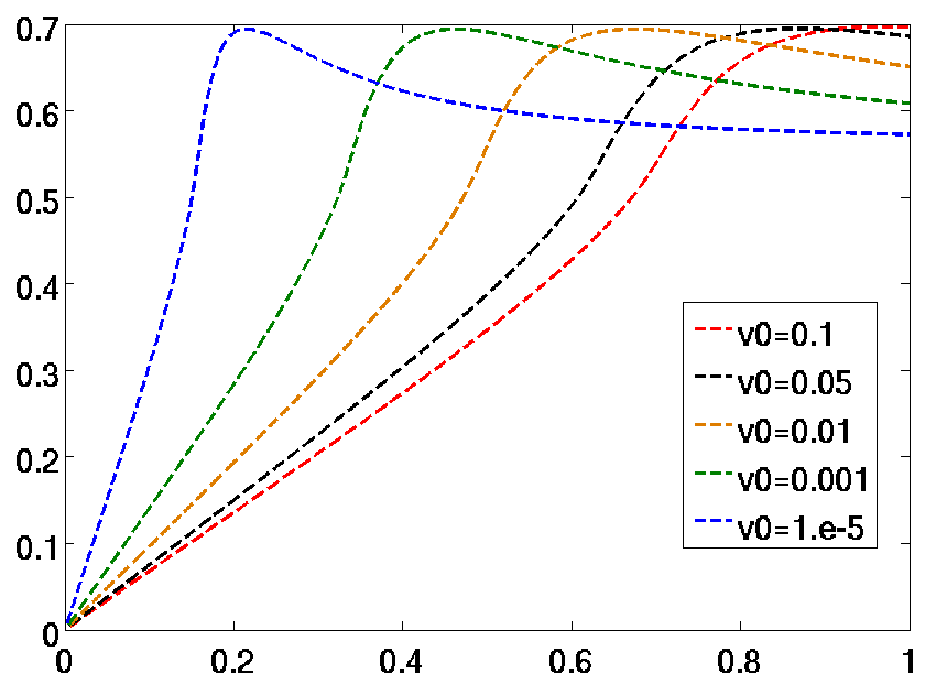
Figure 16: Left: numerical values of $J(v_{0},\rho_{0},\alpha)$ for the smooth function $H_{\rho_{0}}(\rho,\theta)$ given in equation (92). Right: normalized view on the interval $[0,\alpha^{*}(v_{0})]$ for various values of $v_{0}$.

Appendix C Babinet Principle for Acoustic Problems

As mentioned in Section 11.4, for ease of reference, in this appendix we present a derivation of the Babinet principle for scalar waves; see also [7]. Let $\Gamma$ be an open (bounded) flat screen which lies in the $z=0$ plane, and let $u^{i}$ and $u^{s}_{\Gamma}$ denote the incident wave (with sources contained in the semi-space $z<0$), and the corresponding field scattered by $\Gamma$ under the Dirichlet boundary condition given by equation (1) with $f=-u^{i}_{|_{\Gamma}}$. The corresponding total field is denoted as $u^{T}_{\Gamma}=u^{i}+u^{s}_{\Gamma}$.

Calling $\Gamma^{c}$ the complement of $\Gamma$ in the $z=0$ plane, let $v^{s}_{\Gamma^{c}}$ denote the field scattered by $\Gamma^{c}$ under Neumann boundary conditions, and let $v^{T}_{\Gamma^{c}}$ denote the corresponding total field. We now establish the Babinet principle that relates the Dirichlet-screen problem to the Neumann aperture problem, namely

$$u^{T}_{\Gamma}+v^{T}_{\Gamma^{c}}=u^{i}\quad\mbox{for}\quad z>0,$$ (93)

with an associated formula, given below, for $z<0$. The corresponding Babinet principle relating the Neumann-Screen problem to the Dirichlet-aperture problem follows similarly.

In the Dirichlet-screen/Neumann-aperture problem the total field $v^{T}_{\Gamma^{c}}$ satisfies $v^{T}_{\Gamma^{c}}=u^{i}$ on $\Gamma$—since $v^{T}_{\Gamma^{c}}=u^{i}+v^{s}_{\Gamma^{c}}$, and since $v^{s}_{\Gamma^{c}}$ is an odd function of $z$ (as it equals a double-layer potential with source density on $\Gamma^{c}$). Thus, defining $w(x,y,z)=v^{T}_{\Gamma^{c}}(x,y,z)$ for $z>0$, and $w(x,y,z)=v^{T}_{\Gamma^{c}}(x,y,-z)$ for $z<0$, we see that $w$ satisfies the following properties

• The boundary values of $w$ on $\Gamma$ satisfy $w_{|_{\Gamma}}=u^{i}_{|_{\Gamma}}$;

• $w$ is a radiative solution in $\mathbb{R}^{3}$ (since $v^{T}_{\Gamma^{c}}$ is radiating behind the screen)

• $w$ is continuous across $\Gamma^{c}$ (by definition) and its normal derivative across $\Gamma^{c}$ is continuous (since $v^{T}_{\Gamma^{c}}$ satisfies homogeneous Neumann boundary conditions on $\Gamma^{c}$).

It follows that $w=-u^{s}_{\Gamma}$ (by uniqueness of solution to the Dirichlet problem on $\Gamma$) and, therefore, that $v^{T}_{\Gamma^{c}}=-u^{s}_{\Gamma}$ for $z>0$ or, in other words, that $v^{s}_{\Gamma^{c}}=-u^{s}_{\Gamma}-u^{i}$ for $z>0$—and thus equation (93) follows. Since, as stated above, $v^{s}_{\Gamma^{c}}$ is an odd function, its values in the region $z<0$ follow by symmetry.

References

- [1] X. Antoine, A. Bendali, and M. Darbas. Analytic preconditioners for the boundary integral solution of the scattering of acoustic waves by open surfaces. J. Comput. Acoust., 13(3):477–498, 2005.
- [2] I. Babuška and S. Sauter. Is the pollution effect of the FEM avoidable for the Helmholtz equation considering high wave numbers? SIAM Rev., 42(3):451–484, 2000. Reprint of SIAM J. Numer. Anal. 34 (1997), no. 6, 2392–2423 [ MR1480387 (99b:65135)].
- [3] H. A. Bethe. Theory of diffraction by small holes. Phys. Rev. (2), 66:163–182, 1944.
- [4] E. Bleszynski, M. Bleszynski, and T. Jaroszewicz. AIM: Adaptive integral method for solving large-scale electromagnetic scattering and radiation problems. Radio Sci., 31(5):1225–1251, 1996.
- [5] M. Born and E. Wolf. Principles of Optics. Cambridge University Press, seventh edition, 2002.
- [6] C. J. Bouwkamp. On Bethe’s theory of diffraction by small holes. Philips Research Rep., 5:321–332, 1950.
- [7] C. J. Bouwkamp. Diffraction theory. Reports on Progress in Physics, 17:35–100, 1954.
- [8] O. P. Bruno, T. Elling, and Turc C. Regularized integral equations and fast high-order solvers for sound-hard acoustic scattering problems. Int. J. Numer. Meth. Engng., In press, 2012.
- [9] O. P. Bruno and L. Kunyansky. A fast, high-order algorithm for the solution of surface scattering problems: basic implementation, tests, and applications. J. Comput. Phys., 169(1):80–110, 2001.
- [10] O. P. Bruno and S. Lintner. Second-kind integral solvers for TE and TM problems of diffraction by open arcs. Submitted, made available at arxiv.
- [11] S. H. Christiansen and J.-C. Nédélec. Preconditioners for the boundary element method in acoustics. In Mathematical and numerical aspects of wave propagation (Santiago de Compostela, 2000), pages 776–781. SIAM, Philadelphia, PA, 2000.
- [12] D. Colton and R. Kress. Integral Equation Methods in Scattering Theory. John Wiley & Sons, 1983.
- [13] D. Colton and R. Kress. Inverse Acoustic and Electromagnetic Scattering Theory. Springer, 1997.
- [14] L. Jameson. High order schemes for resolving waves: Number of points per wavelength. J. Sci. Comput., 15(4):417–433, 2000.
- [15] S. Lintner and O. P. Bruno. A generalized Calderón formula for open-arc diffraction problems: theoretical considerations. Submitted, available at http://arxiv.org/abs/1204.3699.
- [16] R. Duduchava M. Costabel, M. Dauge. Asymptotics without logarithmic terms for crack problems. Communications in PDE, pages 869–926, 2003.
- [17] A.-W. Maue. Zur Formulierung eines allgemeinen Beugungsproblems durch eine Integralgleichung. Z. Physik, 126:601–618, 1949.
- [18] J. Meixner. Die Kantenbedingung in der Theorie der Beugung elektromagnetischer Wellen an vollkommen leitenden ebenen Schirmen. Ann. Physik (6), 6:2–9, 1949.
- [19] L. Mönch. On the numerical solution of the direct scattering problem for an open sound-hard arc. J. Comput. Appl. Math., 71(2):343–356, 1996.
- [20] JC. Nédélec. Acoustic and electromagnetic equations, volume 144 of Applied Mathematical Sciences. Springer-Verlag, New York, 2001.
- [21] A. Ya. Povzner and I. V. Suharevskiĭ. Integral equations of the second kind in problems of diffraction by an infinitely thin screen. Soviet Physics. Dokl., 4:798–801, 1960.
- [22] W. H. Press, Teukolsky S., W. Vetterling, and B. Flannery. Numerical Recipes in C. Cambridge University Press, 1992. Second Edition.
- [23] V. Rokhlin. Diagonal forms of translation operators for the Helmholtz equation in three dimensions. Appl. Comput. Harmon. Anal., 1(1):82–93, 1993.
- [24] Y. Saad and M. H. Schultz. GMRES: a generalized minimal residual algorithm for solving nonsymmetric linear systems. SIAM J. Sci. Statist. Comput., 7(3):856–869, 1986.
- [25] E. Stephan. Boundary integral equations for screen problems in . Integral Equations Operator Theory, 10(2):236–257, 1987.
- [26] L. Ying, G. Biros, and D. Zorin. A high-order 3D boundary integral equation solver for elliptic PDEs in smooth domains. J. Comput. Phys., 219(1):247–275, 2006.