Stability and convergence analysis of discretizations of the Black–Scholes PDE with the linear boundary condition

Abstract

In this paper we consider the stability and convergence of numerical discretizations of the Black–Scholes partial differential equation (PDE) when complemented with the popular linear boundary condition. This condition states that the second derivative of the option value vanishes when the underlying asset price gets large and is often applied in the actual numerical solution of PDEs in finance. To our knowledge, the only theoretical stability result in the literature up to now pertinent to the linear boundary condition has been obtained by Windcliff, Forsyth & Vetzal [14] who showed that for a common discretization a necessary eigenvalue condition for stability holds. In this paper, we shall present sufficient conditions for stability and convergence when the linear boundary condition is employed. We deal with finite difference discretizations in the spatial (asset) variable and a subsequent implicit discretization in time. As a main result we prove that even though the maximum norm of $e^{tM}$ ($t\geq 0$) can grow with the dimension of the semidiscrete matrix $M$, this generally does not impair the convergence behavior of the numerical discretizations. Our theoretical results are illustrated by ample numerical experiments.

1 Introduction

A popular assumption in the valuation of financial options via the numerical solution of partial differential equations (PDEs) is the so-called linear boundary condition, see, for example, [1, 10, 13, 14]. The linear boundary condition states that the second derivative of the option value with respect to the underlying asset price vanishes if the asset price gets large. This condition represents a linear behavior of the option value for large asset prices, which can be seen to hold for a wide variety of financial options. In spite of its broad use in practice, only few rigorous results have been derived in the literature up to now on the stability and convergence of numerical discretizations if the linear boundary condition is applied. As it turns out, in the finite difference (FD) approach a natural treatment of the linear boundary condition leads to a downwind  discretization of the advection term at the relevant grid point; the details of which are given below in this section. Consequently, in the actual numerical solution one might expect instability, or at least an adverse effect on the convergence behavior. It appears, however, that this is not observed in practice. To our knowledge, the only theoretical stability analysis in the literature up to now pertinent to the linear boundary condition has been performed by Windcliff, Forsyth & Vetzal [14]. These authors proved that for a common discretization of the Black–Scholes PDE a necessary  eigenvalue condition for stability holds. The objective of the present paper is to arrive at useful sufficient conditions for stability and convergence of discretizations when the linear boundary condition is employed. As far as we are aware, such conditions are lacking in the current literature, but they are clearly of much interest.

Consider the Black–Scholes PDE

$$\frac{\partial u}{\partial t}(s,t)=\tfrac{1}{2}\sigma^{2}s^{2}\frac{\partial^{2}u}{\partial s^{2}}(s,t)+rs\frac{\partial u}{\partial s}(s,t)-ru(s,t)\quad(s>0,~{}0<t\leq T),$$ (1.1)

where $r>0$ and $\sigma\geq 0$ are given real constants that denote the risk-neutral interest rate and the volatility, respectively, and $T>0$ is the given maturity time of the option. The exact solution $u(s,t)$ represents the fair value of an option if the underlying asset price equals $s$ at time $T-t$.

For the numerical solution, one restricts in practice the $s$-domain to a boun-ded set $[0,S]$ with fixed $S>0$ chosen sufficiently large. The PDE (1.1) is complemented with initial and boundary conditions. In this paper, we consider at $s=S$ the linear boundary condition

$$u_{ss}(S,t)=0\quad(0<t\leq T).$$ (1.2)

At the lower boundary $s=0$ a standard Dirichlet condition is taken, which depends on the particular option. The initial condition is given by the payoff of the option.

FD discretization of the initial-boundary value problem for (1.1) on a general (non-uniform) grid $0=s_{0}<s_{1}<s_{2}<\ldots<s_{m+1}<s_{m+2}=S$, with mesh widths $h_{j}=s_{j}-s_{j-1}$, leads to an initial value problem for a system of ordinary differential equations (ODEs),

$$U^{\prime}(t)=MU(t)+b(t)\quad(0<t\leq T),\quad U(0)=U_{0}\,.$$ (1.3)

Here $M$ denotes a given real $(m+2)\times(m+2)$–matrix and $U_{0}$ and $b(t)$, for $0\leq t\leq T$, are given real $(m+2)$–vectors. The vector $U_{0}$ is directly given by the payoff function and $b$ depends on the Dirichlet condition at $s=0$. In this paper we shall deal with matrices $M$ of the form

$$M = \left(\begin{array}[]{c|c}A&B\\ \hline\cr&C\end{array}\right)$$ (1.6)

$$= \left(\begin{array}[]{ccccc|cc}\alpha_{1}&\gamma_{1}&&&&&\\ \beta_{2}&\alpha_{2}&\gamma_{2}&&&&\\ &\ddots&\ddots&\ddots&&&\\ &&\beta_{m-1}&\alpha_{m-1}&\gamma_{m-1}&&\\ &&&\beta_{m}&\alpha_{m}&\gamma_{m}&\\ \hline\cr&&&&&-\frac{rS\phantom{\hat{T}}}{h_{m+2}}&\frac{rs_{m+1}}{h_{m+2}}\\ &&&&&-\frac{rS\phantom{\hat{T}}}{h_{m+2}}&\frac{rs_{m+1}}{h_{m+2}}\end{array}\right)$$ (1.14)

where $\alpha_{j}$, $\beta_{j}$, $\gamma_{j}$ denote given real numbers. The $2\times 2$–matrix $C$ represents a natural discretization of the linear boundary condition (1.2). It is determined by the following approximations at the grid points $s_{m+1}$ and $s_{m+2}=S$:

$$u_{s}(s_{m+1},t)\approx\frac{u(s_{m+2},t)-u(s_{m+1},t)}{h_{m+2}}\,,&u_{ss}(s_{m+1},t)\approx 0\,,\\ u_{s}(s_{m+2},t)\approx\frac{u(s_{m+2},t)-u(s_{m+1},t)}{h_{m+2}}\,,u_{ss}(s_{m+2},t)=0\,.$$ (1.15)

As $r$ in (1.1) is positive, the approximation of $u_{s}$ forms an upwind scheme at $s_{m+1}$, but the same approximation constitutes a downwind scheme at $s_{m+2}$. The latter approximation can be regarded as obtained from the second-order central scheme for advection at $s_{m+2}$ with virtual point $s_{m+3}:=s_{m+2}+h_{m+2}$ and then replacing $u(s_{m+3},t)$ by $2u(s_{m+2},t)-u(s_{m+1},t)$ in view of the linear boundary condition. The discretization (1.15b) at $s_{m+2}$ is identical to the one considered in [14]. The discretization (1.15a) at $s_{m+1}$, on the other hand, appears to be new. In particular, we approximate $u_{ss}$ by zero at this point instead of using the standard second-order central scheme for diffusion. The choice (1.15) yields a partial decoupling between the FD solution at the grid points $s_{m+1},s_{m+2}$ and that at $s_{1},s_{2},\ldots,s_{m}$. Concerning the discretization on $[s_{1},s_{m}]$ we make no assumptions yet, except that at each relevant grid point $s_{j}$ the stencil belongs to $\{s_{j-1},s_{j},s_{j+1}\}$ – hence the structure of the matrices $A$ and $B$ in (1.6).

The discretization (1.15) of the linear boundary condition (1.2) might be interpreted as a Dirichlet-type condition, since the relevant subsystem of ODEs involving the matrix $C$ is easily solved exactly (cf. (2.3) below). We emphasize, however, that the objective of this paper concerns comparing the numerical solution to the exact solution of the Black–Scholes PDE with the linear boundary condition (1.2) at the upper boundary $s=S$, and not  with a Dirichlet condition. As it turns out, the analysis in the present situation, of (1.2), encounters a variety of additional difficulties.

Our analysis commences with an investigation of the stability of the FD discretization (1.3), (1.6). This pertains to the derivation of rigorous bounds on the norm of the matrix exponential $e^{tM}$. We shall deal here with the maximum norm. By $|\cdot|_{\infty}$ and $\|\cdot\|_{\infty}$ we denote the maximum norm of real vectors and matrices, respectively. An important tool is the logarithmic maximum norm, which is defined for any square matrix $X$ by

$$\mu_{\infty}[X]=\lim_{t\downarrow 0}\frac{||I+tX||_{\infty}-1}{t}\,,$$

where $I$ is the identity matrix of the same size as $X$. Upon writing $X=(\xi_{ij})_{i,j=1}^{m}$ a convenient formula for the logarithmic maximum norm is

$$\mu_{\infty}[X]=\max_{1\leq i\leq m}\{\,\xi_{ii}+\sum_{j\neq i}|\xi_{ij}|\,\}.$$ (1.16)

A key property is given by the following theorem; see e.g. [3, 7, 9, 11].

Theorem 1.1

Let $\omega\in\mathbb{R}$. Then:   $\mu_{\infty}[X]\leq\omega~{}~{}\Longleftrightarrow~{}~{}||e^{tX}||_{\infty}\leq e^{t\omega}~{}(t\geq 0).$

We note that we previously used the logarithmic norm in analyzing the stability of discretizations of the Black–Scholes and Heston PDEs when provided with Dirichlet boundary conditions, see [5, 6, 12].

An outline of the rest of the paper is as follows.

In Section 2 we investigate the stability of general semidiscretizations (1.3), (1.6) of the Black–Scholes PDE with the linear boundary condition. We prove sharp upper and lower bounds for $||e^{tM}||_{\infty}$.

In Section 3 various well-known FD discretizations are considered. For each discretization a practical sufficient condition is obtained such that the stability result of Section 2 holds.

In Section 4 we derive a convergence estimate for general semidiscretizations (1.3), (1.6) of the Black–Scholes PDE with the linear boundary condition. In Section 2 it was found that $||e^{tM}||_{\infty}$ is essentially inversely proportional to the mesh width $h_{m+2}$. We prove however the positive result that this growth, as $h_{m+2}$ tends to zero, generally has no adverse effect on the convergence behavior.

In Section 5 extensive numerical experiments are presented regarding the stability and convergence results of Sections 2, 4.

In Section 6 we consider the discretization in time and prove stability and convergence results for the popular family of $\theta$-methods. These results can be regarded as analogues of those obtained for the semidiscretization.

In Section 7 conclusions and issues for future research are given.

2 A general stability theorem

In this section we consider general matrices $M$ of the form (1.6) and derive a useful inclusion for the maximum norm of $e^{tM}$ for $t\geq 0$. We start with three lemmas.

Lemma 2.1

It holds that

$$e^{tM}=\left(\begin{array}[]{c|c}e^{tA}&\int_{0}^{t}e^{(t-\tau)A}Be^{\tau C}d\tau\\ \hline\cr O&e^{tC^{\phantom{X}}}\end{array}\right).$$

Proof  Consider the system of ODEs

$$U^{\prime}(t)=MU(t)$$

with solution given by

$$U(t)=e^{tM}U(0).$$ (2.1)

Let the vector $U(t)$ be splitted into two parts,

$$U(t)=\left(\begin{array}[]{c}V(t)\\ W(t)\end{array}\right),$$

where $V(t)$ is an $m$–vector and $W(t)$ is a 2–vector. In view of (1.6) one has

$$\begin{cases}V^{\prime}(t)\,=AV(t)+BW(t),\\ W^{\prime}(t)=CW(t).\end{cases}$$

Thus $W(t)=e^{tC}W(0)$ and

$$V^{\prime}(\tau)-AV(\tau)=Be^{\tau C}W(0)$$

$$\Rightarrow\frac{d}{d\tau}\left(e^{-\tau A}V(\tau)\right)=e^{-\tau A}Be^{\tau C}W(0)$$

$$\Rightarrow e^{-tA}V(t)-V(0)=\int_{0}^{t}e^{-\tau A}Be^{\tau C}W(0)\,d\tau$$

$$\Rightarrow V(t)=e^{tA}V(0)+\int_{0}^{t}e^{(t-\tau)A}Be^{\tau C}\,d\tau\,\,W(0).$$

Comparing with (2.1), the result of the lemma is obtained.

$\Box$

The next lemma gives the maximum norm of $e^{tC}$.

Lemma 2.2

It holds that

$$||e^{tC}||_{\infty}=e^{-rt}+\left(1-e^{-rt}\right)\frac{2S}{h_{m+2}}\,.$$ (2.2)

Proof  The two eigenvalues of $C$ are $0$ and $-r$ with corresponding eigenvectors $(s_{m+1}~{}\,S)^{\rm T}$ and $(1~{}\,1)^{\rm T}$. Thus

$$e^{tC}=\left(\begin{array}[]{cc}s_{m+1}&1\\ S&1\end{array}\right)\left(\begin{array}[]{cc}1&0\\ 0&e^{-rt}\end{array}\right)\left(\begin{array}[]{cc}s_{m+1}&1\\ S&1\end{array}\right)^{-1}$$

which gives

$$e^{tC}=\frac{1}{h_{m+2}}\left(\begin{array}[]{cc}Se^{-rt}-s_{m+1}&s_{m+1}(1-e^{-rt})\\ S(e^{-rt}-1)&S-s_{m+1}e^{-rt}\end{array}\right).$$ (2.3)

Hence,

$$||e^{tC}||_{\infty}=\frac{\max\left\{|Se^{-rt}-s_{m+1}|+s_{m+1}(1-e^{-rt})\,,\,S(1-e^{-rt})+S-s_{m+1}e^{-rt}\right\}}{h_{m+2}}\,.$$

It is readily seen that

$$|Se^{-rt}-s_{m+1}|+s_{m+1}(1-e^{-rt})\leq S(1-e^{-rt})+S-s_{m+1}e^{-rt}.$$

Therefore,

$$||e^{tC}||_{\infty}=\frac{S(1-e^{-rt})+S-s_{m+1}e^{-rt}}{h_{m+2}}=e^{-rt}+\left(1-e^{-rt}\right)\frac{2S}{h_{m+2}}.$$

$\Box$

Lemma 2.2 shows that for any given $t,r,S>0$ the maximum norm of $e^{tC}$ is essentially inversely proportional to the mesh width $h_{m+2}$. The growth of $||e^{tC}||_{\infty}$ as $h_{m+2}$ decreases corresponds to the fact that at the grid point $s=S$ a downwind scheme is used for the advection term in the Black–Scholes PDE.

Let $e_{m}$ denote the $m$–dimensional unit vector $(0,\ldots,0,1)^{\rm T}$.

Lemma 2.3

If $A$ is invertible, $\mu_{\infty}[A]\leq 0$ and $\alpha_{m}+|\beta_{m}|<0$, then

$$|A^{-1}e_{m}|_{\infty}\leq\frac{1}{-\alpha_{m}-|\beta_{m}|}\,.$$

Proof  (i) Consider first $\mu_{\infty}[A]<0$. Define $v=A^{-1}e_{m}$, i.e., $Av=e_{m}$. Writing $v=(v_{1},v_{2},\ldots,v_{m})^{\rm T}$ this gives the system of equations

$$\begin{cases}\alpha_{1}v_{1}+\gamma_{1}v_{2}=0,&\\ \beta_{i}v_{i-1}+\alpha_{i}v_{i}+\gamma_{i}v_{i+1}=0&(2\leq i\leq m-1),\\ \beta_{m}v_{m-1}+\alpha_{m}v_{m}=1.&\end{cases}$$

We prove by induction that $|v_{1}|\leq|v_{2}|\leq\ldots\leq|v_{m}|$. In view of (1.16), the assumptions on $A$ imply that all $\alpha_{i}<0$ and $\alpha_{1}+|\gamma_{1}|<0$. Using this, yields

$$|v_{1}|=\left|\frac{\gamma_{1}}{\alpha_{1}}\right|\cdot|v_{2}|\leq|v_{2}|.$$

Next suppose $|v_{i-1}|\leq|v_{i}|$ for some $2\leq i\leq m-1$. We show that $|v_{i}|\leq|v_{i+1}|$. By (1.16) there holds $|\beta_{i}|+\alpha_{i}+|\gamma_{i}|<0$ and consequently

$$|\alpha_{i}|-|\beta_{i}|>0\quad{\rm and}\quad\frac{|\gamma_{i}|}{|\alpha_{i}|-|\beta_{i}|}<1.$$

We have

$$\beta_{i}v_{i-1}+\alpha_{i}v_{i}+\gamma_{i}v_{i+1}=0$$

$$\Rightarrow\quad |\alpha_{i}|\cdot|v_{i}|\leq|\beta_{i}|\cdot|v_{i-1}|+|\gamma_{i}|\cdot|v_{i+1}|$$

$$\Rightarrow\quad |\alpha_{i}|\cdot|v_{i}|\leq|\beta_{i}|\cdot|v_{i}|+|\gamma_{i}|\cdot|v_{i+1}|$$

$$\Rightarrow\quad |v_{i}|\leq\frac{|\gamma_{i}|}{|\alpha_{i}|-|\beta_{i}|}|v_{i+1}|$$

$$\Rightarrow\quad |v_{i}|\leq|v_{i+1}|.$$

This proves the induction step, and it follows that $|A^{-1}e_{m}|_{\infty}=|v|_{\infty}=|v_{m}|$. Subsequently,

$$\alpha_{m}v_{m}=1-\beta_{m}v_{m-1}$$

$$\Rightarrow\quad |\alpha_{m}|\cdot|v_{m}|\leq 1+|\beta_{m}|\cdot|v_{m-1}|$$

$$\Rightarrow\quad |\alpha_{m}|\cdot|v_{m}|\leq 1+|\beta_{m}|\cdot|v_{m}|$$

$$\Rightarrow\quad |v_{m}|\leq\frac{1}{|\alpha_{m}|-|\beta_{m}|}\,,$$

where it is used that $|\alpha_{m}|-|\beta_{m}|>0$. Since $|\alpha_{m}|=-\alpha_{m}$ the bound of the lemma is obtained.

(ii) Consider next $\mu_{\infty}[A]=0$. Define the matrix $A_{\varepsilon}=A-\varepsilon I$ with $\varepsilon>0$. There holds $\mu_{\infty}[A_{\varepsilon}]=-\varepsilon<0$ and thus we can apply the result from part (i):

$$|A_{\varepsilon}^{-1}e_{m}|_{\infty}\leq\frac{1}{-\alpha_{m}+\varepsilon-|\beta_{m}|}\,.$$

Taking the limit $\varepsilon\downarrow 0$ in this inequality completes the proof.

$\Box$

The following theorem is the first main result of this paper. It provides a tight inclusion of the maximum norm of $e^{tM}$ for matrices $M$ of the form (1.6) and reveals that this norm is essentially inversely proportional to $h_{m+2}$.

Theorem 2.4

If

$$rI+A{\rm~{}is~{}invertible},~{}~{}\mu_{\infty}[rI+A]\leq 0,~{}~{}r+\alpha_{m}+|\beta_{m}|+|\gamma_{m}|\leq 0,$$ (2.4)

then

$$e^{-rt}+\left(1-e^{-rt}\right)\frac{2S}{h_{m+2}}\,\leq\,||e^{tM}||_{\infty}\,\leq\,e^{-rt}+\left(1+3e^{-rt}\right)\frac{2S}{h_{m+2}}\,.$$ (2.5)

Proof  We employ the formula for $e^{tM}$ given by Lemma 2.1. First, it is clear that $||e^{tM}||_{\infty}\geq||e^{tC}||_{\infty}$ and by Lemma 2.2 the lower bound is directly obtained. To prove the stated upper bound, we consider the maximum norm of

$$\int_{0}^{t}e^{(t-\tau)A}Be^{\tau C}d\tau.$$

Using formula (2.3), it is readily shown that

$$Be^{\tau C}=\frac{\gamma_{m}}{h_{m+2}}\left[\begin{array}[]{cc}(Se^{-r\tau}-s_{m+1})e_{m}&(s_{m+1}-s_{m+1}e^{-r\tau})e_{m}\end{array}\right].$$ (2.6)

For any given real numbers $\phi_{0}$, $\phi_{1}$ consider the vector

$$f(\tau)=(\phi_{0}+\phi_{1}e^{-r\tau})e_{m}.$$

A straightforward computation yields

$$\int_{0}^{t}e^{(t-\tau)A}f(\tau)d\tau=\phi_{0}(e^{tA}-I)A^{-1}e_{m}+\phi_{1}(e^{tA}-e^{-rt}I)(rI+A)^{-1}e_{m}.$$

Note that $\mu_{\infty}[rI+A]\leq 0$ means $\mu_{\infty}[A]\leq-r$. In view of this and the assumptions of the theorem it holds that both $A$ and $rI+A$ are invertible and, by Theorem 1.1,

$$||e^{tA}||_{\infty}\leq e^{-rt}.$$ (2.7)

Consequently, we have the bound

$$|\int_{0}^{t}e^{(t-\tau)A}f(\tau)d\tau\,|_{\infty}\leq(1+e^{-rt})\cdot|\phi_{0}|\cdot|A^{-1}e_{m}|_{\infty}+2e^{-rt}\cdot|\phi_{1}|\cdot|(rI+A)^{-1}e_{m}|_{\infty}.$$

Now let $f(\tau)$ represent any column vector of $Be^{\tau C}$. It is clear from (2.6) that

$$|\phi_{0}|\leq|\gamma_{m}|\cdot\frac{S}{h_{m+2}}\quad{\rm and}\quad|\phi_{1}|\leq|\gamma_{m}|\cdot\frac{S}{h_{m+2}}\,.$$

If $\gamma_{m}=0$, then the result of the theorem is obvious; in fact $||e^{tM}||_{\infty}=||e^{tC}||_{\infty}$ in this case. Thus assume $\gamma_{m}\not=0$. Then $r+\alpha_{m}+|\beta_{m}|<0$ and application of Lemma 2.3 to both $A$ and $rI+A$ yields

$$|A^{-1}e_{m}|_{\infty}\leq\frac{1}{-\alpha_{m}-|\beta_{m}|}\quad{\rm and}\quad|(rI+A)^{-1}e_{m}|_{\infty}\leq\frac{1}{-r-\alpha_{m}-|\beta_{m}|}\,.$$

Since

$$\frac{|\gamma_{m}|}{-\alpha_{m}-|\beta_{m}|}\leq 1\quad{\rm and}\quad\frac{|\gamma_{m}|}{-r-\alpha_{m}-|\beta_{m}|}\leq 1.$$

it follows that

$$|\int_{0}^{t}e^{(t-\tau)A}f(\tau)d\tau\,|_{\infty}\leq(1+3e^{-rt})\cdot\frac{S}{h_{m+2}}\,.$$

Using that $Be^{\tau C}$ has two columns, we arrive at the bound

$$\|\int_{0}^{t}e^{(t-\tau)A}Be^{\tau C}d\tau\,\|_{\infty}\leq(1+3e^{-rt})\cdot\frac{2S}{h_{m+2}}\,.$$ (2.8)

Finally, in view of Lemma 2.1,

$$||e^{tM}||_{\infty}\leq\max\left\{||e^{tA}||_{\infty}+\|\int_{0}^{t}e^{(t-\tau)A}Be^{\tau C}d\tau\,\|_{\infty}~{},~{}||e^{tC}||_{\infty}\right\}.$$

By invoking (2.7), (2.8) and Lemma 2.2, the upper bound of the theorem is obtained.

$\Box$

In Section 3, applications of Theorem 2.4 to various actual FD discretizations of the Black–Scholes PDE with the linear boundary condition shall be discussed. In Section 4 the stability results from the present section shall effectively be used in the convergence analysis of FD discretizations.

Remark 2.5

A more direct way to arrive at a bound for $||e^{tM}||_{\infty}$ is by using the inequality

$$\|\int_{0}^{t}e^{(t-\tau)A}Be^{\tau C}d\tau\,\|_{\infty}\leq\int_{0}^{t}||e^{(t-\tau)A}||_{\infty}\cdot||B||_{\infty}\cdot||e^{\tau C}||_{\infty}\,d\tau\\$$

and then applying (2.2), (2.7) and calculating the obtained (simple) integral. However, this leads to an upper bound which is substantially less favorable than that of Theorem 2.4. The reason for this lies in the fact that it yields a factor $|\gamma_{m}|/h_{m+2}$ and in all actual applications the quantity $|\gamma_{m}|$ is itself inversely proportional to one or more mesh widths, cf. Section 3.

In subsequent applications of Theorem 2.4 the following lemma is useful.

Lemma 2.6

If $A$ satisfies the conditions

$$\left\{\begin{array}[]{ll}\beta_{j}\geq 0&(2\leq j\leq m),\\ \gamma_{j}>0&(1\leq j\leq m-1),\\ \alpha_{1}+\gamma_{1}\leq 0,&\hbox{}\\ \alpha_{j}+\beta_{j}+\gamma_{j}=0&(2\leq j\leq m-1),\\ \alpha_{m}+\beta_{m}<0,&\hbox{}\end{array}\right.$$

then $A$ is invertible and $\mu_{\infty}[A]=0$.

Proof  The conditions of the lemma directly imply, by (1.16), that $\mu_{\infty}[A]=0$. We next show that $A$ is invertible. Upon setting $\beta_{1}=-\alpha_{1}-\gamma_{1}\geq 0$ and $\gamma_{m}=-\alpha_{m}-\beta_{m}>0$ and using that $\alpha_{j}+\beta_{j}+\gamma_{j}\equiv 0$ we obtain

$$\left(\begin{array}[]{cccccc}\alpha_{1}&\gamma_{1}\\ \beta_{2}&\alpha_{2}&\gamma_{2}\\ &\ddots&\ddots&\ddots\\ &&\ddots&\ddots&\ddots\\ &&&\beta_{m-1}&\alpha_{m-1}&\gamma_{m-1}\\ &&&&\beta_{m}&\alpha_{m}\end{array}\right)\cdot\left(\begin{array}[]{cccccc}1\\ 1&1\\ \vdots&\vdots&\ddots\\ \vdots&\vdots&&\ddots\\ 1&1&\ldots&\ldots&1\end{array}\right)=$$

$$\left(\begin{array}[]{cccccc}-\beta_{1}&\gamma_{1}\\ &-\beta_{2}&\gamma_{2}\\ &&\ddots&\ddots\\ &&&\ddots&\ddots\\ &&&&-\beta_{m-1}&\gamma_{m-1}\\ \hline\cr-\gamma_{m}&-\gamma_{m}&\ldots&\ldots&-\gamma_{m}&\alpha_{m}\end{array}\right)=:P\,.$$

Next, modify the matrix $P$ by subtracting column 1 from columns $2,3,\ldots,m-1$. This leads to

$$\widetilde{P}=\left(\begin{array}[]{cccccc|c}-\beta_{1}&-\alpha_{1}&\beta_{1}&\beta_{1}&\ldots&\beta_{1}&\\ \hline\cr&-\beta_{2}&\gamma_{2}&&&&\\ &&-\beta_{3}&\gamma_{3}&&&\\ &&&\ddots&\ddots&&\\ &&&&-\beta_{m-2}&\gamma_{m-2}&\\ &&&&&-\beta_{m-1}&\gamma_{m-1}\\ \hline\cr-\gamma_{m}&&&&&&\alpha_{m}\end{array}\right).$$

Clearly, if $\widetilde{P}$ is invertible, then so is $A$. We prove that

$$x\in\mathbb{R}^{m}\,,\,\widetilde{P}x=0~{}\Longrightarrow~{}x=0.$$

Write $x=(x_{1},x_{2},\ldots,x_{m})^{\rm T}$. Then $\widetilde{P}x=0$ is equivalent to the system of equations

$$\begin{cases}-\beta_{1}x_{1}-\alpha_{1}x_{2}+\beta_{1}x_{3}+\beta_{1}x_{4}+\ldots+\beta_{1}x_{m-1}\phantom{+\gamma_{m-1}x_{m}}&=\,0\\ \phantom{-\beta_{1}x_{1}}-\beta_{2}x_{2}+\gamma_{2}x_{3}\phantom{+\beta_{1}x_{4}+\ldots+\beta_{1}x_{m-1}}&=\,0\\ \phantom{-\beta_{1}x_{1}-\alpha_{1}x_{2}}-\beta_{3}x_{3}+\gamma_{3}x_{4}\phantom{+\ldots+\beta_{1}x_{m-1}}&=\,0\\ \phantom{-\beta_{1}x_{1}-\alpha_{1})_{2}-\beta_{3}x_{3}+\gamma_{3}x_{4}}\quad\ddots&\quad\vdots\\ \phantom{-\beta_{1}x_{1}-\alpha_{1}x_{2}+\beta_{1}x_{3}+\beta_{1}x_{4}+\ddots}-\beta_{m-1}x_{m-1}+\gamma_{m-1}x_{m}&=\,0\\ -\gamma_{m}x_{1}\phantom{-\alpha_{1}x_{2}+\beta_{1}x_{3}+\beta_{1}x_{4}+\ldots-\beta_{m-1}x_{m-1}+}+\alpha_{m}x_{m}&=\,0.\end{cases}$$ (2.9)

We distinguish three cases.

(a) Assume $\beta_{j}\not=0$ whenever $1\leq j\leq m$. Then $\alpha_{j}<0$, $\beta_{j}>0$, $\gamma_{j}>0$ for all $j$. Starting with the last equation of (2.9) and moving upwards, one finds that

$$x_{m}=\frac{\gamma_{m}}{\alpha_{m}}\,x_{1}\,,\quad x_{j}=\left(\prod_{k=j}^{m-1}\frac{\gamma_{k}}{\beta_{k}}\right)\frac{\gamma_{m}}{\alpha_{m}}\,x_{1}\qquad(2\leq j\leq m-1).$$

Substituting this into the first equation of (2.9) yields

$$\left[-\beta_{1}-\alpha_{1}\left(\prod_{k=2}^{m-1}\frac{\gamma_{k}}{\beta_{k}}\right)\frac{\gamma_{m}}{\alpha_{m}}+\beta_{1}\sum_{j=3}^{m-1}\left(\prod_{k=j}^{m-1}\frac{\gamma_{k}}{\beta_{k}}\right)\frac{\gamma_{m}}{\alpha_{m}}\right]x_{1}=0.$$

It is easily seen that the coefficient of $x_{1}$ in the latter equation is nonzero. Thus $x_{1}=0$, and consequently $x=0$.

(b) Assume $\beta_{1}=0$. Since $\alpha_{1}$ and all $\gamma_{j}$ are nonzero, (2.9) directly yields that $x=0$.

(c) Assume $\beta_{j}=0$ for certain $2\leq j\leq m$. This induces a natural partitioning of the matrix $A$ where each diagonal block belongs to either case (a) or case (b) above. Using this, it readily follows that if $Ax=0$ then $x=0$.

$\Box$

Remark 2.7

Under the assumptions of Lemma 2.6 it holds that $-A$ is a so-called M-matrix. This follows, e.g., by using condition $({\rm M}_{37})$ in [2, Chapter 6].

3 Application of the general stability analysis

In the following we apply the general stability analysis of Section 2 to actual FD discretizations of the Black–Scholes PDE with the linear boundary condition. Pertinent to the advection term on $[s_{1},s_{m}]$ we consider three FD schemes:

$$u_{s}(s_{j},t)&\approx\frac{u(s_{j+1},t)-u(s_{j},t)}{h_{j+1}}\,,\\ u_{s}(s_{j},t)\approx\frac{u(s_{j+1},t)-u(s_{j-1},t)}{H_{j}}\,,\\ u_{s}(s_{j},t)\approx-\frac{h_{j+1}}{h_{j}H_{j}}u(s_{j-1},t)+\frac{h_{j+1}-h_{j}}{h_{j}h_{j+1}}u(s_{j},t)+\frac{h_{j}}{h_{j+1}H_{j}}u(s_{j+1},t).\qquad~{}~{}$$ (3.1)

The scheme (3.1a) has a first-order truncation error and is called the first-order forward scheme. The scheme (3.1b) possesses a second-order truncation error whenever the grid is smooth; for the scheme (3.1c) this holds for arbitrary grids. We refer to (3.1b) and (3.1c) as the central scheme A and the central scheme B, respectively. Notice that these two schemes are identical if the grid is uniform. For the diffusion term on $[s_{1},s_{m}]$ we use the standard central FD scheme

$$u_{ss}(s_{j},t)\approx\frac{2}{h_{j}H_{j}}u(s_{j-1},t)-\frac{2}{h_{j}h_{j+1}}u(s_{j},t)+\frac{2}{h_{j+1}H_{j}}u(s_{j+1},t)\,,$$ (3.2)

which possesses a second-order truncation error on smooth grids.

Based on (3.1), (3.2) we consider five well-known FD discretizations of the Black–Scholes PDE. These discretizations differ in the treatment of the advection term $rsu_{s}$ on the interval $[s_{1},s_{m}]$. The linear boundary condition is always discretized on $[s_{m+1},s_{m+2}]$ according to (1.15). For each semidiscretization, successive application of Lemma 2.6 (with $A$ replaced by $rI+A$) and Theorem 2.4 directly gives a condition on $r$, $\sigma$ and the grid such that the stability bound (2.5) holds.

1. Forward.  Using the first-order forward scheme gives for $1\leq j\leq m$,

   $$\begin{cases}\beta_{j}=\sigma^{2}\displaystyle\frac{s_{j}^{2}}{h_{j}H_{j}}\,,\\ \alpha_{j}=-r-r\displaystyle\frac{s_{j}}{h_{j+1}}-\sigma^{2}\displaystyle\frac{s_{j}^{2}}{h_{j}h_{j+1}}\,,\\ \gamma_{j}=r\displaystyle\frac{s_{j}}{h_{j+1}}+\sigma^{2}\frac{s_{j}^{2}}{h_{j+1}H_{j}}\,.\end{cases}$$ (3.3)

   The bound (2.5) holds for all $r>0$, $\sigma\geq 0$ and all grids.

2. Central A.  Using the central scheme A gives for $1\leq j\leq m$,

   $$\begin{cases}\beta_{j}=-r\displaystyle\frac{s_{j}}{H_{j}}+\sigma^{2}\displaystyle\frac{s_{j}^{2}}{h_{j}H_{j}}\,,\\ \alpha_{j}=-r-\sigma^{2}\displaystyle\frac{s_{j}^{2}}{h_{j}h_{j+1}}\,,\\ \gamma_{j}=r\displaystyle\frac{s_{j}}{H_{j}}+\sigma^{2}\displaystyle\frac{s_{j}^{2}}{h_{j+1}H_{j}}\,.\end{cases}$$ (3.4)

   The bound (2.5) holds if for all $1\leq j\leq m$:

   $$0<r\leq\frac{s_{j}}{h_{j}}\sigma^{2}.$$ (3.5)

3. Central B.  Using the central scheme B gives for $1\leq j\leq m$,

   $$\begin{cases}\beta_{j}=-r\displaystyle\frac{s_{j}h_{j+1}}{h_{j}H_{j}}+\sigma^{2}\displaystyle\frac{s_{j}^{2}}{h_{j}H_{j}}\,,\\ \alpha_{j}=-r+r\displaystyle\frac{s_{j}(h_{j+1}-h_{j})}{h_{j}h_{j+1}}-\sigma^{2}\displaystyle\frac{s_{j}^{2}}{h_{j}h_{j+1}}\,,\\ \gamma_{j}=r\displaystyle\frac{s_{j}h_{j}}{h_{j+1}H_{j}}+\sigma^{2}\displaystyle\frac{s_{j}^{2}}{h_{j+1}H_{j}}\,.\end{cases}$$ (3.6)

   The bound (2.5) holds if for all $1\leq j\leq m$:

   $$0<r\leq\frac{s_{j}}{h_{j+1}}\sigma^{2}.$$ (3.7)

4. Mixed A.  This scheme is defined as a suitable combination of Forward and Central A above. For each given $1\leq j\leq m$: if (3.5) is fulfilled, then define $\alpha_{j}$, $\beta_{j}$, $\gamma_{j}$ by (3.4); else by (3.3). This scheme has been considered e.g. in [14]. Clearly, the idea is to switch from the central scheme (3.4) to the forward scheme (3.3) in those grid points that would give rise to a strictly positive logarithmic maximum norm of $rI+A$. By construction, it follows that the bound (2.5) holds for all $r>0$, $\sigma\geq 0$ and all grids.

5. Mixed B.  This scheme is defined as a suitable combination of Forward and Central B above. For each given $1\leq j\leq m$: if (3.7) is fulfilled, then define $\alpha_{j}$, $\beta_{j}$, $\gamma_{j}$ by (3.6); else by (3.3). Again, it follows that the bound (2.5) holds for all $r>0$, $\sigma\geq 0$ and all grids.

4 A general convergence result

In this section we prove a convergence result for general semidiscretizations (1.3), (1.6) of the Black–Scholes PDE with the linear boundary condition. Let $U$ be the exact solution to (1.3), (1.6) and, for $0\leq t\leq T$, let $u_{h}(t)$ be the vector of the same size as $U(t)$ given by

$$u_{h}(t)=(u(s_{1},t),u(s_{2},t),\ldots,u(s_{m+2},t))^{\rm T}\,,$$

where $u$ is the exact solution to the initial-boundary value problem for the Black–Scholes PDE (1.1) on $0\leq s\leq S$ with linear boundary condition (1.2). Define the spatial discretization error

$$\varepsilon_{h}(t)=u_{h}(t)-U(t)$$

and the spatial truncation error

$$\delta_{h}(t)=u_{h}^{\prime}(t)-Mu_{h}(t)-b(t).$$

A standard approach to estimate spatial discretization errors is to combine an estimate for the spatial truncation errors with a stability bound, cf. e.g. [7]. However, a direct use of the bound on $||e^{tM}||_{\infty}$ from Theorem 2.4 does not lead to an optimal result. To obtain a useful result in the present situation where the linear boundary condition is employed, we consider a partitioning of the spatial truncation error vector into two parts, corresponding to the intervals $[s_{1},s_{m}]$ and $[s_{m+1},s_{m+2}]$:

$$\delta_{h}(t)=\left(\begin{array}[]{c}\delta_{h}^{L}(t)\vspace{0.1cm}\\ \delta_{h}^{R}(t)\\ \end{array}\right)\quad{\rm with}~{}~{}\delta_{h}^{L}(t)\in\mathbb{R}^{m}~{}~{}{\rm and}~{}~{}\delta_{h}^{R}(t)\in\mathbb{R}^{2}.$$

Using the individual stability bounds derived in Section 2, we have as a preliminary result

Lemma 4.1

Assume (2.4) holds. Then the spatial discretization error satisfies

$$|\varepsilon_{h}(t)|_{\infty}\leq t\cdot\max_{0\leq\vartheta\leq t}\left\{|\delta_{h}^{L}(\vartheta)|_{\infty}+\frac{8S}{h_{m+2}}\cdot|\delta_{h}^{R}(\vartheta)|_{\infty}\right\}\quad(t>0).$$

Proof  From

$$u_{h}^{\prime}(t) = Mu_{h}(t)+b(t)+\delta_{h}(t),$$

$$U^{\prime}(t) = MU(t)+b(t)$$

one has

$$\varepsilon_{h}^{\prime}(t)=M\varepsilon_{h}(t)+\delta_{h}(t)~{}~{}~{}~{}~{}~{}~{}~{}~{}$$

and, since $\varepsilon_{h}(0)=0$,

$$\varepsilon_{h}(t)=\int_{0}^{t}e^{(t-\vartheta)M}\delta_{h}(\vartheta)d\vartheta.$$

Lemma 2.1 yields

$$e^{(t-\vartheta)M}\delta_{h}(\vartheta)=\left(\begin{array}[]{c|c}e^{(t-\vartheta)A}&\int_{0}^{t-\vartheta}e^{(t-\vartheta-\tau)A}Be^{\tau C}d\tau\\ \hline\cr O&e^{{(t-\vartheta)C}^{\phantom{X}}}\end{array}\right)\left(\begin{array}[]{c}\delta_{h}^{L}(\vartheta)\vspace{0.1cm}\\ \delta_{h}^{R}(\vartheta)\end{array}\right).$$

By (2.7), (2.8) and Lemma 2.2 the following bounds hold whenever $0\leq\vartheta\leq t$ :

$$||e^{(t-\vartheta)A}||_{\infty} \leq 1,$$

$$||\int_{0}^{t-\vartheta}e^{(t-\vartheta-\tau)A}Be^{\tau C}d\tau||_{\infty} \leq \frac{8S}{h_{m+2}}\,,$$

$$||e^{(t-\vartheta)C}||_{\infty} \leq \frac{2S}{h_{m+2}}\,.$$

Hence

$$|e^{(t-\vartheta)M}\delta_{h}(\vartheta)|_{\infty}\leq|\delta_{h}^{L}(\vartheta)|_{\infty}+\frac{8S}{h_{m+2}}\cdot|\delta_{h}^{R}(\vartheta)|_{\infty}.$$

Together with the integral representation above, this gives the bound on the maximum norm of $\varepsilon_{h}(t)$.

$\Box$

The following theorem forms the second main result of this paper. It gives a useful convergence estimate for general semidiscretizations (1.3), (1.6) of the Black–Scholes PDE with linear boundary condition. Its proof is obtained by combining Lemma 4.1 with a bound for $\delta_{h}^{R}$.

Theorem 4.2

Let $h^{\ast}>0$ be given and assume that on $[S-h^{\ast},S]\times[0,T]$ the partial derivative $u_{sss}$ exists and is continuous. Define

$$\kappa=4\sigma^{2}S^{3}+6rS^{2}h^{\ast}~{}~{}{\it and}~{}~{}\eta(t)=\max\{|u_{sss}(\xi,t)|:S-h^{\ast}\leq\xi\leq S\}.$$ (4.1)

Assume (2.4) holds. Then the spatial discretization error satisfies

$$|\varepsilon_{h}(t)|_{\infty}\leq t\cdot\max_{0\leq\vartheta\leq t}\left\{|\delta_{h}^{L}(\vartheta)|_{\infty}+\kappa\eta(\vartheta)\right\}\quad{\it whenever}~{}0<h_{m+2}\leq h^{\ast},~{}0<t\leq T.$$

Proof Write $s=s_{m+1}$ and $h=h_{m+2}$. Pertinent to the point $s_{m+1}$ we have

$$\delta_{h,1}^{R}(t) = u_{t}(s,t)-rs\,\frac{u(S,t)-u(s,t)}{h}+ru(s,t)$$

$$= \tfrac{1}{2}\sigma^{2}s^{2}u_{ss}(s,t)+rs\,\left[u_{s}(s,t)-\frac{u(S,t)-u(s,t)}{h}\right].$$

By Taylor’s theorem and using $u_{ss}(S,t)=0$ there follows

$$u(s,t) = u(S,t)-hu_{s}(S,t)+E_{0}(h,t),$$

$$u_{s}(s,t) = u_{s}(S,t)+E_{1}(h,t),$$

$$u_{ss}(s,t) = E_{2}(h,t),$$

where

$$E_{0}(h,t)=-\tfrac{1}{6}h^{3}\,u_{sss}(\xi_{0},t)~{},~{}~{}E_{1}(h,t)=\tfrac{1}{2}h^{2}\,u_{sss}(\xi_{1},t)~{},~{}~{}E_{2}(h,t)=-h\,u_{sss}(\xi_{2},t)$$

with certain $\xi_{0},\xi_{1},\xi_{2}$ in $(s,S)$. Substitution into the above formula yields

$$\delta_{h,1}^{R}(t)=\tfrac{1}{2}\sigma^{2}s^{2}E_{2}(h,t)+rsE_{1}(h,t)+\frac{rs}{h}E_{0}(h,t),$$

which readily leads to the estimate

$$|\delta_{h,1}^{R}(t)|\leq\{\tfrac{1}{2}\sigma^{2}S^{2}+\tfrac{2}{3}rSh\}\eta(t)\cdot h.$$

Analogously, pertinent to the point $s_{m+2}$, there holds

$$\delta_{h,2}^{R}(t) = u_{t}(S,t)-rS\,\frac{u(S,t)-u(s,t)}{h}+ru(S,t)$$

$$= rS\,\left[u_{s}(S,t)-\frac{u(S,t)-u(s,t)}{h}\right]$$

$$= \frac{rS}{h}E_{0}(h,t)$$

and

$$|\delta_{h,2}^{R}(t)|\leq\tfrac{1}{6}rS\eta(t)\cdot h^{2}.$$

It thus follows that

$$|\delta_{h}^{R}(t)|_{\infty}\leq\{\tfrac{1}{2}\sigma^{2}S^{2}+\tfrac{2}{3}rSh^{\ast}\}\eta(t)\cdot h$$

and

$$\frac{8S}{h}\cdot|\delta_{h}^{R}(t)|_{\infty}\leq\kappa\eta(t).$$ (4.2)

Application of Lemma 4.1 then gives the desired estimate for $|\varepsilon_{h}(t)|_{\infty}$.

$\Box$

The estimate of Theorem 4.2 for the spatial discretization error consists of two contributions, corresponding to the two intervals $[s_{1},s_{m}]$ and $[s_{m+1},s_{m+2}]$. The first contribution is equal to the part of the spatial truncation error pertinent to $[s_{1},s_{m}]$. For any given FD discretization this can be estimated in a standard way by Taylor expansion. The second contribution is equal to $\kappa\eta(\vartheta)$ and depends on the partial derivative $u_{sss}$ of the exact option price near $s=S$. For a wide range of financial options it is plausible that this contribution can be made arbitrarily small upon taking the upper bound $S$ sufficiently large (in the case of European call and put options this is readily proved). Theorem 4.2 thus expresses the useful result that the contribution to spatial discretization error of the semidiscretized linear boundary condition is negligible, provided $S$ is sufficiently large. Key to the proof is that the stability bounds derived in Section 2 admit a growth of errors from the interval $[s_{m+1},s_{m+2}]$ that is at most inversely proportional to $h_{m+2}$ but this growth is precisely offset by the factor $h_{m+2}$ that arises in the part of the spatial truncation error pertinent to this interval.

We note that in Theorem 4.2 it is tacitly assumed that the initial function is smooth, which has been used for ease of the analysis, but is often not fulfilled in applications. The numerical experiments in the subsequent section deal with a nonsmooth initial function.

5 Numerical experiments

In this section the stability and convergence results of Sections 2, 4 are illustrated by numerical experiments. We consider the five FD discretizations of the Black–Scholes PDE formulated in Section 3 with the linear boundary condition discretized as given in Section 1. For each FD discretization, we also consider its analogue where the definition of $\alpha_{j}$, $\beta_{j}$, $\gamma_{j}$ for $1\leq j\leq m$ in Section 3 is extended to $j=m+1$. This corresponds to the approach by Windcliff, Forsyth & Vetzal [14] where in the penultimate grid point $s_{m+1}$ no modified discretization is applied related to the linear boundary condition. In the following we shall refer by LBC1 to the numerical treatment of the linear boundary condition as defined in Section 1 and by LBC2 to the treatment as considered in [14].

For the numerical experiments a typical smooth, non-uniform spatial grid is chosen. Let $E\in(0,S)$ and $c>0$ be given and fixed. Consider the continuous, strictly increasing function

$$\varphi(\xi)=E+c\cdot\sinh(\xi)\quad(a\leq\xi\leq b)$$

with $a=\sinh^{-1}(-E/c)$ and $b=\sinh^{-1}((S-E)/c)$. Let

$$\xi_{j}=a+j\cdot\Delta\xi\quad(0\leq j\leq m+2)~{}~{}~{}\textrm{with}~{}~{}\Delta\xi=\frac{b-a}{m+2}.$$

Then a non-uniform grid $0=s_{0}<s_{1}<\ldots<s_{m+1}<s_{m+2}=S$ is defined by the transformation

$$s_{j}=\varphi(\xi_{j})\quad(0\leq j\leq m+2).$$

The parameter $E$ can be viewed as the exercise price of a vanilla option and $c$ determines the fraction of grid points $s_{j}$ that lie in the neighborhood of $E$,

$$h_{j}\approx c\cdot\Delta\xi\quad\textrm{whenever}~{}~{}s_{j}\approx E.$$

The grid is smooth in the sense that there exist real constants $c_{0}$, $c_{1}$, $c_{2}>0$ (independent of $j$ and $m$) such that the mesh widths $h_{j}$ satisfy

$$c_{0}\cdot\Delta\xi\leq h_{j}\leq c_{1}\cdot\Delta\xi\quad\textrm{and}\quad|h_{j+1}-h_{j}|\leq c_{2}\cdot(\Delta\xi)^{2}.$$

The above type of grid is often used in financial applications, cf. e.g. [5, 10]. We (arbitrarily) set $E=100$, $c=E/5$, $S=400$.

5.1 Stability experiments

First, the stability of the ten FD discretizations discussed above is numerically investigated. For each FD discretization we consider the maximum of $||e^{tM}||_{\infty}$ over $t\geq 0$ for the dimensions $m=50,100,\ldots,1000$. We employed the Matlab function expm to evaluate the matrix exponential and computed the values of $||e^{tM}||_{\infty}$ for $t=0,1,\ldots,100$; this was found to give a reliable estimate for the maximum over all $t\geq 0$. For the experiments three pairs $r,\sigma$ have been chosen. Figure 1 displays the obtained results. On the top row $r=0.1$ and $\sigma=0.3$; on the middle row $r=0.3$ and $\sigma=0.1$; on the bottom row $r=0.2$ and $\sigma=0$. The left column represents the LBC1 treatment of the linear boundary condition and the right column represents the LBC2 treatment. Note that the scales on the vertical axes vary.

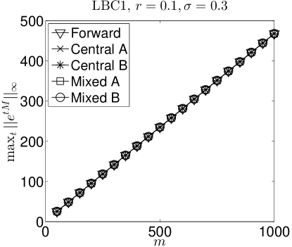
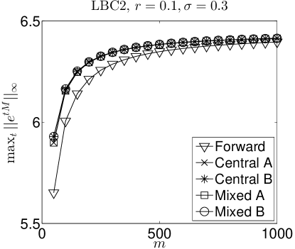
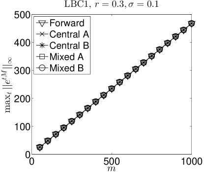
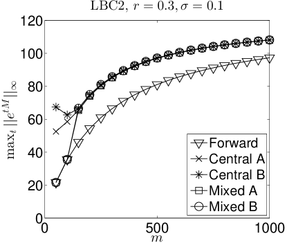
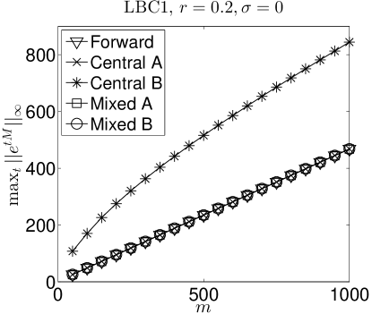
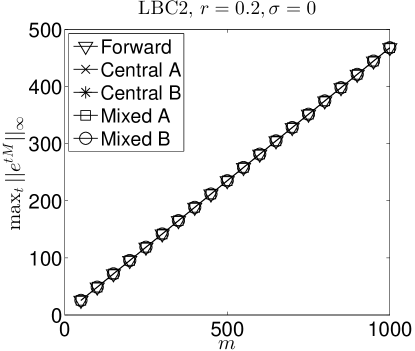
Figure 1: Plot of $\max\{||e^{tM}||_{\infty}:t=0,1,\ldots,100\}$ vs. $m=50,100,\ldots,1000$. On the top row $r=0.1$ and $\sigma=0.3$; on the middle row $r=0.3$ and $\sigma=0.1$; on the bottom row $r=0.2$ and $\sigma=0$. The left column concerns the LBC1 discretization of the linear boundary condition; the right column concerns the LBC2 discretization. In all cases $E=100$ and $S=400$. Notice the different scales on the vertical axes.

If $r=0.1$ and $\sigma=0.3$, then the Mixed A and B discretizations are identical to Central A and B, respectively; in this case the conditions (3.5), (3.7) always hold. On the other hand, if $r=0.2$ and $\sigma=0$, then Mixed A and B both reduce to the Forward discretization; in this case (3.5), (3.7) never hold. Finally, if $r=0.3$ and $\sigma=0.1$, then Mixed A and B form an actual mix of Forward with Central A and B, respectively.

Considering the left column of Figure 1, a main observation is that the results for the Forward and the Mixed A and B discretizations with the LBC1 treatment agree with the stability bound (2.5) given by Theorem 2.4. Indeed, for all $r$, $\sigma$ pairs the maximum of $||e^{tM}||_{\infty}$ over $t$ is found to be directly proportional to $m$, and moreover,

$$\max_{t\geq 0}||e^{tM}||_{\infty}\approx\frac{2S}{h_{m+2}}\,.$$ (5.1)

If $r=0.1$ and $\sigma=0.3$, then the results for Central A and B with LBC1 clearly also agree with (2.5), as these discretizations coincide with Mixed A and B. We do not have a theoretical stability result for the central discretizations for the other two $r$, $\sigma$ pairs, but it is interesting that the estimate (5.1) is also observed in the left column for Central A and B if $r=0.3$ and $\sigma=0.1$, and for Central A if $r=0.2$ and $\sigma=0$. Although (5.1) is not found for Central B in the latter case, the maximum of $||e^{tM}||_{\infty}$ over $t$ still appears to be at most directly proportional to $m$.

Considering the right column of Figure 1, we observe in the top and middle rows that for all five FD discretizations with the LBC2 treatment there appears to be an upper bound on $||e^{tM}||_{\infty}$ that is uniform both in $t$ and the dimension $m$. This upper bound is small in the top row and larger in the middle row. It appears to increase if the ratio $\sigma^{2}/r$ decreases. In the limit case of $\sigma=0$, displayed in the bottom row, one obtains again linear growth with $m$ for the Forward and Mixed A and B discretizations with LBC2. In fact, it is readily seen that these three discretizations then all reduce to Forward with LBC1. We notice that similar observations as here concerning LBC2 were made in [14].

If $\sigma=0$, then the results for the Central A and B discretizations with LBC2 are not displayed in the figure. For each considered dimension $m$, the obtained maximum of $||e^{tM}||_{\infty}$ is very large in this case. For example, if $m=100$, then the maximum values (over $t=0,1,\ldots,100$) for Central A and B are equal to $2.5\times 10^{3}$ and $1.5\times 10^{5}$, respectively, and if $m=200$, then they are equal to $9.8\times 10^{3}$ and $5.8\times 10^{5}$. In fact, there appears to be growth with $m^{2}$.

When $\sigma$ is not small, then comparing the results in the left and right columns of Figure 1 one may be inclined to prefer the LBC2 treatment over LBC1: for both $r$, $\sigma$ pairs with nonzero $\sigma$ one observes, for each given FD discretization, that the maximum of $||e^{tM}||_{\infty}$ is more favorable for LBC2 compared to LBC1. However, considering the actual convergence behavior of the FD discretizations, we find no essential difference between the two treatments, as is illustrated next.

5.2 Convergence experiments

Here we numerically examine the convergence behavior of the ten FD discretizations of the Black–Scholes PDE with linear boundary condition discussed above. For the experiments we consider a European call option with exercise price $E$, so that

$$u(s,0)=\max(0,s-E)\quad(s\geq 0),~{}~{}~{}u(0,t)=0\quad(0\leq t\leq T),$$

and set $E=100$, $T=5$, $S=2000$. In the experiments we compute the maximum norm of the spatial discretization errors

$$e_{h}(T)=u_{h}(T)-U(T)$$

for a sequence of values $m$ with $10^{2}\leq m\leq 10^{4}$. Here $u_{h}$ denotes the restriction to the spatial grid of the exact call option price function, given by the Black–Scholes formula. The semidiscrete solution vector $U(T)$ to (1.3), (1.6) is approximated, with sufficiently high accuracy, by applying the Crank–Nicolson method using $N=10^{4}$ time steps. In view of the nonsmooth initial condition, two initial (damping) substeps are taken with the implicit Euler method. This approach is often referred to as Rannacher time stepping.

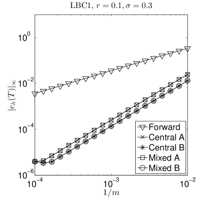
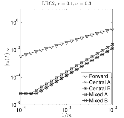
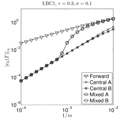
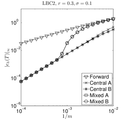
Figure 2: Plot of $|e_{h}(T)|_{\infty}$ vs. $1/m$  for values $10^{2}\leq m\leq 10^{4}$ equally spaced on a logarithmic scale. On the top row $r=0.1$ and $\sigma=0.3$; on the bottom row $r=0.3$ and $\sigma=0.1$. The left column concerns the LBC1 discretization of the linear boundary condition; the right column concerns the LBC2 discretization. In all cases $E=100$, $T=5$, $S=2000$.

The results are displayed in Figure 2. On the first row $r=0.1$, $\sigma=0.3$ and on the second row $r=0.3$, $\sigma=0.1$. The left column represents the LBC1 treatment of the linear boundary condition and the right column represents the LBC2 treatment.

As a first observation it is clear that LBC1 and LBC2 almost always lead to the same spatial discretization error in the experiments.

If $r=0.1$ and $\sigma=0.3$, then the Mixed A and B discretizations are identical to Central A and B, respectively. For these four discretizations we find, by least-squares approximation in the region $m\leq 5000$, an order of convergence equal to 2.0. Once $m$ gets larger than 5000, then the (fixed) error due to the linear boundary condition dominates. The Forward discretization has an observed order of convergence equal to 1.0.

If $r=0.3$ and $\sigma=0.1$ the observed orders of convergence are 0.9 for Forward, 2.0 for Central A and 1.9 for Central B. The Mixed A and B discretizations are in this case an actual mix of Forward with Central A and B, respectively. Table 1 gives for each $m$ under consideration the fraction of grid points where the Forward discretization is used. Clearly, for small $m$ this fraction is large and Mixed A and B show spatial discretization errors similar to those for Forward, whereas for large $m$ this fraction is small and Mixed A and B show errors similar to those for the Central A and B discretizations. A rigorous analysis of this correlation will be left for future research.

$m$	Fraction Mixed A	Fraction Mixed B
100	57.0%	58.0%
129	47.3%	48.8%
167	34.1%	36.5%
215	9.8%	11.2%
278	7.9%	7.6%
359	6.4%	6.4%
464	5.2%	5.2%
599	4.2%	4.2%
774	3.4%	3.4%
1000	2.7%	2.7%
1292	2.1%	2.1%
1668	1.7%	1.7%
2154	1.3%	1.3%
2783	1.0%	1.0%
3594	0.8%	0.8%
4642	0.6%	0.6%
5995	0.5%	0.5%
7743	0.4%	0.4%
10000	0.3%	0.3%

Table 1: Fraction of grid points where the Forward discretization is used in Mixed A and Mixed B vs. $m$  in the case of $r=0.3$, $\sigma=0.1$ and LBC1.

6 Time discretization

In this section we study the time discretization of the semidiscrete system (1.3), (1.6) by the well-known family of $\theta$-methods, which includes the popular Crank–Nicolson method (trapezoidal rule) and implicit Euler method as special cases. As noted in Section 1, the subsystem of ODEs involving the matrix $C$ could be solved exactly, but it is more interesting and useful, both from a theoretical and practical point of view, to consider the time discretization of the semidiscrete system (1.3), (1.6) as a whole.

Let parameter $\theta\in[\tfrac{1}{2},1]$ be given and fixed. Let step size $\Delta t=T/N$ with integer $N\geq 1$ be given and define $t_{n}=n\,\Delta t$, $b_{n}=b(t_{n})$ for $n=0,1,2,\ldots,N$. The $\theta$-method generates, in a successive way, for $n=1,2,\ldots,N$ an approximation $U_{n}$ to $U(t_{n})$ by

$$U_{n}=U_{n-1}+(1-\theta)\,\Delta t\,(MU_{n-1}+b_{n-1})+\theta\,\Delta t\,(MU_{n}+b_{n}).$$

The choices $\theta=\frac{1}{2}$ and $\theta=1$ yield, respectively, the Crank–Nicolson method and implicit Euler method. The above recurrence relation can be written as

$$U_{n}=\varphi(\Delta t\,M)U_{n-1}+(I-\theta\Delta t\,M)^{-1}[(1-\theta)\,\Delta t\,b_{n-1}+\theta\,\Delta t\,b_{n}],$$ (6.1)

where $\varphi$ is the so-called stability function of the method, given by

$$\varphi(z)=\frac{1+(1-\theta)z}{1-\theta z}\quad({\rm for}~{}z\in\mathbb{C}),$$

and

$$\varphi(X)=(I-\theta X)^{-1}(I+(1-\theta)X)=(I+(1-\theta)X)(I-\theta X)^{-1}$$

for square matrices $X$ such that $I-\theta X$ is invertible.

We first study the stability of the fully discrete process (6.1). The subsequent two lemmas can be viewed as analogues of Lemmas 2.1, 2.2 for the semidiscrete system.

Lemma 6.1

For $1\leq n\leq N$ there holds

$$\varphi(\Delta t\,M)^{n}=\left(\begin{array}[]{c|c}\varphi(\Delta t\,A)^{n}&Y_{n}\\ \hline\cr O&\varphi(\Delta t\,C)^{n}\end{array}\right)$$

where

$$Y_{1}&=(I-\theta\Delta t\,A)^{-1}\Delta t\,B(I-\theta\Delta t\,C)^{-1},\\ Y_{n}=\sum_{j=0}^{n-1}\,\varphi(\Delta t\,A)^{n-j-1}\,Y_{1}\,\varphi(\Delta t\,C)^{j}.$$ (6.2)

Proof  The formula is readily obtained by induction to $n$ and noting that

$$(I-\theta\Delta t\,M)^{-1}=\left(\begin{array}[]{c|c}(I-\theta\Delta t\,A)^{-1}&\theta\,Y_{1}\\ \hline\cr O&(I-\theta\Delta t\,C)^{-1}\end{array}\right).$$ (6.3)

$\Box$

Lemma 6.2

For $1\leq n\leq N$ there holds

$$||\varphi(\Delta t\,C)^{n}||_{\infty}=x^{n}+\left(1-x^{n}\right)\frac{2S}{h_{m+2}}\quad{\it with}~{}~{}x=\varphi(-r\Delta t).$$

Proof With the eigendecomposition of $C$ it is easily verified that

$$\varphi(\Delta t\,C)^{n}=\frac{1}{h_{m+2}}\left(\begin{array}[]{cc}Sx^{n}-s_{m+1}&s_{m+1}(1-x^{n})\\ S(x^{n}-1)&S-s_{m+1}x^{n}\end{array}\right)$$

and the rest of the proof is similar to that of Lemma 2.2, using $|x|\leq 1$.

$\Box$

Concerning the discretization on the spatial domain $[s_{1},s_{m}]$ we shall assume in the following that there exists a real constant $K$, independent of the dimension $m$ and number of time steps $n$, such that

$$||\varphi(\Delta t\,A)^{n}||_{\infty}\leq K\quad{\rm whenever}~{}~{}\Delta t=T/N,~{}0\leq n\leq N,~{}N\geq 1.$$ (6.4)

In the literature much attention has been paid to establishing (6.4), under a variety of conditions on the matrix $A$. For the implicit Euler method ($\theta=1$) the neat result is well-known that (6.4) is fulfilled with $K=1$ whenever $\mu_{\infty}[A]\leq 0$, cf. e.g. [4, 8]. Hence, this is guaranteed under the condition (2.4). For all other time discretization methods, however, the available results in the literature implying (6.4) with a constant $K$ independent of $m$ and $n$ require, to the best of our knowledge, stronger conditions on $A$. Notably, conditions on the resolvent, the numerical range and pseudospectra have been extensively investigated in the literature, cf. e.g. [9, 11]. Some of these results appear to be useful in our current application, but a verification of the pertinent conditions on $A$ is highly non-trivial. As our main interest in this paper lies in studying (the implications of) the discretized linear boundary condition on $[s_{m+1},s_{m+2}]$, which corresponds to the matrices $B$ and $C$, we shall leave the analysis of (6.4) when $\tfrac{1}{2}\leq\theta<1$ for future research.

The next theorem can be regarded as a discrete analogue to Theorem 2.4.

Theorem 6.3

If  (2.4) and (6.4) then for $1\leq n\leq N$,

$$x^{n}+\left(1-x^{n}\right)\frac{2S}{h_{m+2}}\,\leq\,||\varphi(\Delta t\,M)^{n}||_{\infty}\,\leq\,K+\frac{4(K+1)S}{h_{m+2}}$$

with $x=\varphi(-r\Delta t)$.

Proof  For any integer $j\geq 0$, let the rational function $\psi_{j}$ be defined by

$$\psi_{j}(z)=\frac{\varphi(z)^{j}}{1-\theta z}\quad(z\in\mathbb{C}).$$

Consider the formula for $\varphi(\Delta t\,M)^{n}$ given by Lemma 6.1. The lower bound on its maximum norm is clear by Lemma 6.2. To prove the upper bound, write

$$Y_{n} = \sum_{j=0}^{n-1}\,\varphi(\Delta t\,A)^{n-j-1}\,(I-\theta\Delta t\,A)^{-1}\Delta t\,B\,(I-\theta\Delta t\,C)^{-1}\varphi(\Delta t\,C)^{j}$$

$$= \sum_{j=0}^{n-1}\,\varphi(\Delta t\,A)^{n-j-1}\,(I-\theta\Delta t\,A)^{-1}\Delta t\,B\,\psi_{j}(\Delta t\,C).$$

It holds that

$$B\,\psi_{j}(\Delta t\,C)=\frac{\gamma_{m}}{h_{m+2}}\left[\begin{array}[]{cc}(Sx_{j}-s_{m+1})e_{m}&(s_{m+1}-s_{m+1}x_{j})e_{m}\end{array}\right]$$ (6.5)

where $x_{j}=\psi_{j}(-r\Delta t)\in[-1,1]$. Both columns of this matrix are of the form

$$f_{j}=(\phi_{0}+\phi_{1}x_{j})e_{m}$$

with real numbers $\phi_{0}$, $\phi_{1}$ independent of $j$.

We have

$$\Delta t\,\sum_{j=0}^{n-1}\,\varphi(\Delta t\,A)^{n-j-1}\,(I-\theta\Delta t\,A)^{-1}$$

$$=\Delta t\,\sum_{k=0}^{n-1}\,\varphi(\Delta t\,A)^{k}\,(I-\theta\Delta t\,A)^{-1}$$

$$=\Delta t\,(\varphi(\Delta t\,A)^{n}-I)(\varphi(\Delta t\,A)-I)^{-1}(I-\theta\Delta t\,A)^{-1}$$

$$=\Delta t\,(\varphi(\Delta t\,A)^{n}-I)(I+(1-\theta)\Delta t\,A-I+\theta\Delta t\,A)^{-1}$$

$$=(\varphi(\Delta t\,A)^{n}-I)A^{-1}.$$

By similar algebraic manipulations, there follows

$$\Delta t\,\sum_{j=0}^{n-1}\,\varphi(\Delta t\,A)^{n-j-1}\,(I-\theta\Delta t\,A)^{-1}x_{j}$$

$$=(\varphi(\Delta t\,A)^{n}-\varphi(-r\Delta t)^{n}I)(rI+A)^{-1}.$$

Consequently,

$$\Delta t\,\sum_{j=0}^{n-1}\,\varphi(\Delta t\,A)^{n-j-1}\,(I-\theta\Delta t\,A)^{-1}f_{j}$$ (6.6)

$$=\phi_{0}\,(\varphi(\Delta t\,A)^{n}-I)A^{-1}e_{m}+\phi_{1}\,(\varphi(\Delta t\,A)^{n}-\varphi(-r\Delta t)^{n}I)(rI+A)^{-1}e_{m}.$$

Continuing from here along the same lines as in the proof of Theorem 2.4, and using the condition (6.4), we arrive at

$$||Y_{n}||_{\infty}\leq\frac{4(K+1)S}{h_{m+2}}\,.$$

Together with Lemma 6.2, the stated upper bound on $||\varphi(\Delta t\,M)^{n}||_{\infty}$ now directly follows.

$\Box$

In the subsequent convergence analysis of the process (6.1), the matrix

$$\psi_{n}(\Delta t\,M)=\varphi(\Delta t\,M)^{n}(I-\theta\Delta t\,M)^{-1}$$

arises. By Lemma 6.1 and formula (6.3),

$$\psi_{n}(\Delta t\,M)=\left(\begin{array}[]{c|c}\psi_{n}(\Delta t\,A)&\theta\,\varphi(\Delta t\,A)^{n}\,Y_{1}+Y_{n}\,(I-\theta\Delta t\,C)^{-1}\\ \hline\cr O&\psi_{n}(\Delta t\,C)\end{array}\right).$$

For the analysis below we need upper bounds on the maximum norms of the constituent submatrices. Putting $Y_{0}=O$, there holds

Lemma 6.4

If  (2.4) and (6.4) then for $0\leq n\leq N-1$,

$$||\psi_{n}(\Delta t\,A)||_{\infty}&\leq K\,,\phantom{\frac{4S}{h_{m+2}}}\\ ||\psi_{n}(\Delta t\,C)||_{\infty}\leq\frac{4S}{h_{m+2}}\,,\\ ||\varphi(\Delta t\,A)^{n}\,Y_{1}||_{\infty}\leq\frac{4KS}{h_{m+2}}\,,\\ ||Y_{n}\,(I-\theta\Delta t\,C)^{-1}||_{\infty}\leq\frac{4(K+1)S}{h_{m+2}}\,.$$ (6.7)

Proof The bound (6.7a) follows directly from (6.4) and the fact that (2.4) implies $||(I-\theta\Delta t\,A)^{-1}||_{\infty}\leq 1$. The bound (6.7b) is obtained using the same arguments as in the proof of Lemma 6.2. In order to prove (6.7c) we note that

$$(I-\theta\Delta t\,A)^{-1}=(\varphi(\Delta t\,A)-I)(\Delta t\,A)^{-1}$$

and using this gives

$$\varphi(\Delta t\,A)^{n}\,Y_{1}=(\varphi(\Delta t\,A)^{n+1}-\varphi(\Delta t\,A)^{n})\,A^{-1}B\,(I-\theta\Delta t\,C)^{-1}.$$ (6.8)

By (6.5) with $j=0$,

$$B\,(I-\theta\Delta t\,C)^{-1}=\frac{\gamma_{m}}{h_{m+2}}\left[\begin{array}[]{cc}(Sx_{0}-s_{m+1})e_{m}&(s_{m+1}-s_{m+1}x_{0})e_{m}\end{array}\right]$$

where $x_{0}=(1+\theta\,r\Delta t)^{-1}\in(0,1)$. If $f_{0}$ represents any of the two columns of this matrix, then by a same argument as in the proof of Theorem 2.4 there follows

$$|A^{-1}f_{0}|_{\infty}\leq\frac{S}{h_{m+2}}\,.$$

Consequently,

$$||(\varphi(\Delta t\,A)^{n+1}-\varphi(\Delta t\,A)^{n})\,A^{-1}B\,(I-\theta\Delta t\,C)^{-1}||_{\infty}\leq 2K\cdot 2\cdot\frac{S}{h_{m+2}}=\frac{4KS}{h_{m+2}}\,.$$

The proof of the bound (6.7d) is identical to that for $||Y_{n}||_{\infty}$ given above, except that $\psi_{j}(z)$ needs to be replaced by $\psi_{j}(z)/(1-\theta z)$.

$\Box$

To prove the convergence result for the time discretization process (6.1), we also need the following result.

Lemma 6.5

Assume (2.4) and (6.4) hold. Let $g:[0,S]\rightarrow\mathbb{R}$ be any given continuously differentiable function and

$$w=\left(\begin{array}[]{c}g(s_{m+1})\\ g(s_{m+2})\\ \end{array}\right)\in\mathbb{R}^{2}.$$

Then there exists $\xi\in(s_{m+1},s_{m+2})$ such that for all $0\leq n\leq N-1$:

$$|\psi_{n}(\Delta t\,C)\,w|_{\infty}&\leq|g(S)|+2S|g^{\prime}(\xi)|,\\ \\ |\varphi(\Delta t\,A)^{n}\,Y_{1}\,w|_{\infty}\leq 2K(|g(S)|+S|g^{\prime}(\xi)|),\\ \\ |Y_{n}\,(I-\theta\Delta t\,C)^{-1}\,w|_{\infty}\leq(K+1)(|g(S)|+2S|g^{\prime}(\xi)|).$$ (6.9)

Proof Write $s=s_{m+1}$ and $h=h_{m+2}$. Let $\xi\in(s,S)$ be such that

$$g(s)=g(S)-hg^{\prime}(\xi).$$

Then the vector $w$ can be written as

$$w=g(S)\left(\begin{array}[]{c}1\\ 1\\ \end{array}\right)-hg^{\prime}(\xi)\left(\begin{array}[]{c}1\\ 0\\ \end{array}\right).$$

For any rational function $\psi$ with $\psi(0)=1$ there holds

$$\psi(\Delta t\,C)=\frac{1}{h}\left(\begin{array}[]{cc}Sx-s&s(1-x)\\ S(x-1)&S-sx\end{array}\right)$$

where $x=\psi(-r\Delta t)$. Application of this matrix to $w$, in the above form, readily yields

$$\psi(\Delta t\,C)w=\left(\begin{array}[]{c}g(S)x-g^{\prime}(\xi)(Sx-s)\\ g(S)x-g^{\prime}(\xi)(Sx-S)\\ \end{array}\right).$$

Observe the important fact that there is no factor $1/h$ present here.

(a) The bound (6.9a) is obtained upon taking $\psi=\psi_{n}$ and using $|x|\leq 1$.

(b) By formula (6.8),

$$|\varphi(\Delta t\,A)^{n}\,Y_{1}\,w|_{\infty}\leq 2K\cdot|A^{-1}B\,(I-\theta\Delta t\,C)^{-1}\,w|_{\infty}.$$

Considering $\psi(z)=\psi_{0}(z)=(1-\theta z)^{-1}$ yields

$$A^{-1}B\,(I-\theta\Delta t\,C)^{-1}\,w=(g(S)x-g^{\prime}(\xi)(Sx-s))\,\gamma_{m}\,A^{-1}e_{m}$$

with $x=(1+\theta\,r\Delta t)^{-1}$. As in the proof of Theorem 2.4 we have $|\gamma_{m}\,A^{-1}e_{m}|_{\infty}\leq 1$ and, together with $0<x<1$, there follows

$$|A^{-1}B\,(I-\theta\Delta t\,C)^{-1}\,w|_{\infty}\leq|g(S)|+S|g^{\prime}(\xi)|,$$

which completes the proof of (6.9b).

(c) By formula (6.2),

$$Y_{n}(I-\theta\Delta t\,C)^{-1}\,w=\sum_{j=0}^{n-1}\,\varphi(\Delta t\,A)^{n-j-1}\,(I-\theta\Delta t\,A)^{-1}\Delta t\,B\,{\widetilde{\psi}}_{j}(\Delta t\,C)w$$

with ${\widetilde{\psi}}_{j}(z)=\psi_{j}(z)/(1-\theta z)$. Taking $\psi={\widetilde{\psi}}_{j}$ in the above general formula, we get

$$B\,{\widetilde{\psi}}_{j}(\Delta t\,C)w=(\phi_{0}+\phi_{1}{\widetilde{x}}_{j})e_{m},$$

where

$${\widetilde{x}}_{j}={\widetilde{\psi}}_{j}(-r\Delta t)~{}~{},~{}~{}\phi_{0}=\gamma_{m}\,g^{\prime}(\xi)s~{}~{},~{}~{}\phi_{1}=\gamma_{m}\,(g(S)-g^{\prime}(\xi)S).$$

It is convenient to set $x_{j}=\psi_{j}(-r\Delta t)$ and ${\widetilde{\phi}}_{1}=\phi_{1}/(1+\theta\,r\Delta t)$. Then $\phi_{1}{\widetilde{x}}_{j}={\widetilde{\phi}}_{1}x_{j}$ and formula (6.6) directly gives

$$Y_{n}(I-\theta\Delta t\,C)^{-1}\,w$$

$$=\Delta t\,\sum_{j=0}^{n-1}\,\varphi(\Delta t\,A)^{n-j-1}\,(I-\theta\Delta t\,A)^{-1}(\phi_{0}+\phi_{1}{\widetilde{x}}_{j})e_{m}$$

$$=\phi_{0}\,(\varphi(\Delta t\,A)^{n}-I)A^{-1}e_{m}+{\widetilde{\phi}}_{1}\,(\varphi(\Delta t\,A)^{n}-\varphi(-r\Delta t)^{n}I)(rI+A)^{-1}e_{m}.$$

Using that $|\gamma_{m}\,A^{-1}e_{m}|_{\infty}\leq 1$ and $|\gamma_{m}\,(rI+A)^{-1}e_{m}|_{\infty}\leq 1$ yields

$$|Y_{n}\,(I-\theta\Delta t\,C)^{-1}\,w|_{\infty} \leq (K+1)(|g^{\prime}(\xi)|S+|g(S)-g^{\prime}(\xi)S|)$$

$$\leq (K+1)(|g(S)|+2S|g^{\prime}(\xi)|),$$

which proves the bound (6.9c).

$\Box$

As in Section 4, let the vector $u_{h}(t)$ be given by

$$u_{h}(t)=(u(s_{1},t),u(s_{2},t),\ldots,u(s_{m+2},t))^{\rm T}\,,$$

where $u$ is the exact solution to the initial-boundary value problem for the Black–Scholes PDE (1.1) on $0\leq s\leq S$ with linear boundary condition (1.2). The following theorem provides a useful estimate for the space-time discretization error, defined by

$${\widehat{\varepsilon}}_{n}=u_{h}(t_{n})-U_{n}\quad(0\leq n\leq N).$$

It essentially states that the estimate for the spatial discretization error from Theorem 4.2 remains valid after time discretization up to a  $c\cdot(\Delta t)^{p}$ term, where $p$ denotes the classical order of consistency of the $\theta$-method and $c$ is a constant independent of the spatial grid and the time step.

Theorem 6.6

Let $p=1$ if  $\tfrac{1}{2}<\theta\leq 1$ and $p=2$ if  $\theta=\tfrac{1}{2}$. Assume that all partial derivatives of $u$ of orders $\leq p+2$ exist and are continuous on $[0,S]\times[0,T]$. Let $h^{\ast}>0$ be given and let $\kappa$, $\eta$ be defined by (4.1). Assume (2.4) and (6.4) hold. Then there exists a real constant $c$ (depending only on $u$, $S$, $\theta$ and $K$) such that

$$|{\widehat{\varepsilon}}_{n}|_{\infty}\leq t_{n}\cdot\left\{K\cdot\max_{0\leq\vartheta\leq t_{n}}|\delta_{h}^{L}(\vartheta)|_{\infty}+(K+\tfrac{1}{2})\kappa\cdot\max_{0\leq\vartheta\leq t_{n}}\eta(\vartheta)+c\cdot(\Delta t)^{p}\right\}$$

whenever  $0<h_{m+2}\leq h^{\ast}$, $\Delta t=T/N$, $1\leq n\leq N$, $N\geq 1$.

Proof Let the local space-time error ${\widehat{\delta}}_{n}$ in the $n$-th step of (6.1) be defined by

$$u_{h}(t_{n})=\varphi(\Delta t\,M)u_{h}(t_{n-1})+(I-\theta\Delta t\,M)^{-1}[(1-\theta)\,\Delta t\,b_{n-1}+\theta\,\Delta t\,b_{n}]+{\widehat{\delta}}_{n}.$$

Subtracting (6.1) from this yields

$${\widehat{\varepsilon}}_{n}=\varphi(\Delta t\,M){\widehat{\varepsilon}}_{n-1}+{\widehat{\delta}}_{n}=\ldots=\sum_{j=1}^{n}\varphi(\Delta t\,M)^{n-j}\,{\widehat{\delta}}_{j}.$$ (6.10)

With the spatial truncation error

$$\delta_{h}(t)=\left(\begin{array}[]{c}\delta_{h}^{L}(t)\vspace{0.1cm}\\ \delta_{h}^{R}(t)\\ \end{array}\right)$$

as defined in Section 4, one can express $b(t)$ as

$$b(t)=u_{h}^{\prime}(t)-Mu_{h}(t)-\delta_{h}(t).$$

Inserting this into the definition of ${\widehat{\delta}}_{j}$ it readily follows that

$${\widehat{\delta}}_{j}&=(I-\theta\Delta t\,M)^{-1}[(1-\theta)\,\Delta t\,\delta_{h}(t_{j-1})+\theta\,\Delta t\,\delta_{h}(t_{j})]+\\ (I-\theta\Delta t\,M)^{-1}[u_{h}(t_{j})-u_{h}(t_{j-1})-(1-\theta)\,\Delta t\,u_{h}^{\prime}(t_{j-1})-\theta\,\Delta t\,u_{h}^{\prime}(t_{j})].$$ (6.11)

The above formula for ${\widehat{\delta}}_{j}$ consists of two terms, corresponding to the truncation error in space and the truncation error in time. In view of (6.10), we shall study $\varphi(\Delta t\,M)^{n-j}\,{\widehat{\delta}}_{j}$.

Concerning the first term, the bounds for the submatrices of $\psi_{n-j}(\Delta t\,M)=\varphi(\Delta t\,M)^{n-j}\,(I-\theta\Delta t\,M)^{-1}$ given by Lemma 6.4 directly lead to

$$|\psi_{n-j}(\Delta t\,M)\,[(1-\theta)\,\Delta t\,\delta_{h}(t_{j-1})+\theta\,\Delta t\,\delta_{h}(t_{j})]\,|_{\infty}~{}\leq$$

$$\Delta t\cdot\left\{K\cdot\max_{l=j-1,j}|\delta_{h}^{L}(t_{l})|_{\infty}+\frac{4(2K+1)S}{h_{m+2}}\cdot\max_{l=j-1,j}|\delta_{h}^{R}(t_{l})|_{\infty}\right\}.$$

Invoking the estimate (4.2) for $\delta_{h}^{R}$ this gives

$$|\psi_{n-j}(\Delta t\,M)\,[(1-\theta)\,\Delta t\,\delta_{h}(t_{j-1})+\theta\,\Delta t\,\delta_{h}(t_{j})]\,|_{\infty}~{}\leq$$

$$\Delta t\cdot\left\{K\cdot\max_{l=j-1,j}|\delta_{h}^{L}(t_{l})|_{\infty}+{\widehat{\kappa}}\cdot\max_{l=j-1,j}|\eta(t_{l})|_{\infty}\right\},$$

where ${\widehat{\kappa}}=(K+\tfrac{1}{2})\kappa$.

Concerning the second term, for the function $g:[0,S]\rightarrow\mathbb{R}$ defined by

$$g(s)=u(s,t_{j})-u(s,t_{j-1})-(1-\theta)\,\Delta t\,u_{t}(s,t_{j-1})-\theta\,\Delta t\,u_{t}(s,t_{j})$$

standard Taylor expansion shows that

$$|g(s)|\leq c_{0}(\Delta t)^{p+1}~{}~{},~{}~{}|g^{\prime}(s)|\leq c_{1}(\Delta t)^{p+1}\quad(0\leq s\leq S)$$

with

$$p=1~{},~{}~{}c_{0}=\tfrac{3}{2}||u_{tt}||_{\infty}~{},~{}~{}~{}~{}c_{1}=\tfrac{3}{2}||u_{stt}||_{\infty}\quad~{}~{}({\rm if~{}}\tfrac{1}{2}<\theta\leq 1),$$

$$p=2~{},~{}~{}c_{0}=\tfrac{5}{12}||u_{ttt}||_{\infty}~{},~{}~{}c_{1}=\tfrac{5}{12}||u_{sttt}||_{\infty}\quad({\rm if~{}}\theta=\tfrac{1}{2}),$$

where $||\cdot||_{\infty}$ designates the maximum norm of a real function on $[0,S]\times[0,T]$. Using now Lemma 6.5 and the partitioning

$$u_{h}(t)=\left(\begin{array}[]{c}v_{h}(t)\vspace{0.1cm}\\ w_{h}(t)\\ \end{array}\right)\quad{\rm with}~{}~{}v_{h}(t)\in\mathbb{R}^{m}~{}~{}{\rm and}~{}~{}w_{h}(t)\in\mathbb{R}^{2},$$

it follows that

$$|\psi_{n-j}(\Delta t\,M)\,[u_{h}(t_{j})-u_{h}(t_{j-1})-(1-\theta)\,\Delta t\,u_{h}^{\prime}(t_{j-1})-\theta\,\Delta t\,u_{h}^{\prime}(t_{j})]|_{\infty}\leq c\,(\Delta t)^{p+1}$$

with

$$c=(4K+1)c_{0}+(4K+2)Sc_{1}.$$

Combining the above bounds, we are led to

$$|{\widehat{\varepsilon}}_{n}|_{\infty} \leq \sum_{j=1}^{n}|\varphi(\Delta t\,M)^{n-j}\,{\widehat{\delta}}_{j}|_{\infty}$$

$$\leq \sum_{j=1}^{n}\Delta t\cdot\left\{K\cdot\max_{l=j-1,j}|\delta_{h}^{L}(t_{l})|_{\infty}+{\widehat{\kappa}}\cdot\max_{l=j-1,j}|\eta(t_{l})|_{\infty}+c\,(\Delta t)^{p}\right\}$$

$$\leq t_{n}\cdot\left\{K\cdot\max_{0\leq\vartheta\leq t_{n}}|\delta_{h}^{L}(\vartheta)|_{\infty}+{\widehat{\kappa}}\cdot\max_{0\leq\vartheta\leq t_{n}}\eta(\vartheta)+c\,(\Delta t)^{p}\right\}.$$

$\Box$

7 Conclusions

In this paper we have analyzed the stability and convergence of discretizations, both in space and time, of the Black–Scholes PDE when it is provided with the linear boundary condition. This condition states that the second derivative of the option value vanishes when the underlying asset price gets large. For the space discretization we considered finite difference schemes and for the time discretization the well-known family of $\theta$-methods. Concerning stability, we derived tight inclusions for the maximum norm of $e^{tM}$ and $\varphi(\Delta t\,M)^{n}$ where the matrix $M$ represents the semidiscretized Black–Scholes PDE operator, $\varphi$ denotes the stability function of the $\theta$-method, time $t\geq 0$, step size $\Delta t>0$ and integer $n\geq 0$. The obtained inclusions reveal that these norms can grow essentially directly proportional to the dimension of the matrix $M$, i.e., the number of spatial grid points. We subsequently proved the positive result that this growth has in general no adverse effect on the convergence behavior of the discretizations.

In future research, in addition to the issues already mentioned previously, we wish to extend the analysis to the discretization of the linear boundary condition that was considered by Windcliff, Forsyth & Vetzal [14]. Also we aim at studying more advanced, multi-dimensional PDEs in finance, such as the Heston PDE, as well as other discretizations in space and time.