Components of multifractality in the Central England Temperature anomaly series

Abstract

We study the multifractal nature of the Central England Temperature (CET) anomaly, a time series that spans more than 200 years. The data are analyzed in two ways: as a single set and by using a sliding window of 11 years. In both cases, we quantify the width of the multifractal spectrum as well as its components, which are defined by the deviations from the Gaussian distribution and the dependence between measurements. The results of the first approach show that the key contribution to the multifractal structure comes from the dynamical dependencies, mainly weak ones, followed by a residual contribution of the deviations from the Gaussian. The sliding window approach indicates that the peaks in the evolution of the non-Gaussian contribution occur almost at the same dates associated with climate changes that were determined in previous works using component analysis methods. Moreover, the strong non-Gaussian contribution from the 1960s onwards is in agreement with global results recently presented.

The finding of self-similar and self-affine traits, namely with multiple scaling exponents, is presently as frequent as the verification of scale-dependence was in the early 20th century. The identification of scale-invariant properties has been crucial to the accurate interpretation and modeling of a long list of problems whereon climate and its dynamics rank high. Despite being frequently studied, there is still much debate on the validity of this concept in order to characterize the behavior of a time series as well as the importance of each ingredient yielding scale invariance, namely dynamical dependencies and non-Gaussianity. Moreover, the nonstationarity of most of the signals and the time-dependence of each contribution to the scale-invariance properties have been systematically overlooked, particularly in the case of the temperature anomaly in climatic time series.

I Introduction

The interest of the scientific community in systems exhibiting self-similarity, i.e., the property whereby a system is (approximately) equal to a part of itself, has increased ever since Mandelbrot introduced the concept of fractality mandelbrot . In fact, aiming at analyzing the existence of scale-invariant behavior, fractals have been applied to such diverse fields as physiology and economics. Generically, scale invariance (or self-similarity) can be characterized by a sole fractal (or Haussdorf) dimension or a spectrum of locally dependent exponents, the so-called multifractal spectrum mfbooks1 ; mfbooks2 ; mfbooks3 . Considering an abstract observable, $\mathcal{O}$, scale invariance (self-similarity) features can be mathematically written as,

$$f\left(\left\{\lambda\,\mathcal{O}^{z}\right\}\right)=\lambda^{\alpha\left(z\right)}\,f\left(\left\{\mathcal{O}\right\}\right),$$ (1)

so that when $\alpha(z)$ is constant for all $z$, the system has a single scale invariant behavior. In the case of a time series, the multifractal concept is prominently self-affine, i.e, it has different scaling properties in the ordinate ($\mathcal{O}$) and abscissa (time) directions.

In the fields of climate science and geophysics, fractality and scale invariance are popular concepts as well. Moreover, the (multi-)fractal nature of meteorological times series and its connection to the widely discussed issue of climatic change has been explored in several studies including instrumental kurnaz ; alvarez and paleoclimaticmf_dfa_appl3 ; bodri ; karimova temperature records and precipitation datavalencia ; rubalcaba . However, the large majority of the surveys on self-similarity in climate data have only been devoted to the analysis of memory effects dyer ; bain ; lovejoy ; matyas ; pelletier in the form of linear dependencies, i.e, dependencies detected when the Pearson correlation function is computed. In that case, the existence of memory in the data is quantified by the power spectrum exponent $\beta$, which is related to a single value of $\alpha$ and that coincides with the Hurst exponent $H$. The value of $\alpha$ relates to the power spectrum exponent $\beta$ via the Wiener-Khinchin relation and the fractal dimension, $D$ reading $D=2-H$. When $\alpha(z)$ is not constant, it is possible to go beyond standard memory effects and explore a wider range of statistical and dynamical properties.

In this manuscript we shed light on the multi-self-similar nature of a well-known long meteorological time series: the anomaly of the Central England Temperature (CET), which is the longest instrumental daily data set available on this subject. The temperature anomaly is the difference between an element of the time series and its long-term average, i.e. the deviation of the daily temperature from its annual cycle. Specifically, our work seeks to provide quantitative answers to the following questions: i) To what extent does the CET anomaly series show real multifractality? ii) What is the weight of each contributing mechanism to the multifractality we measure? ii) Does the relative weight of these contributions change in time? If so, how and why do these changes occur? How much has been the relative magnitude of the changes? Does this dynamics have to do with climate change?

The present manuscript is organized as follows: in Sec. II we provide a thorough description of the data analyzed and the methods we employed; in Sec. III we present our results concerning the proposed questions, and in Sec. IV we discuss the results and present some conclusions we are able to draw from our analysis.

II Data and Methods

II.1 The Central England Temperature time series

The Central England Temperature (CET) is the longest instrumental time series, starting in 1772. Owing to its large span, it can be used to perform comparisons between the pre-industrial era, during which the emission of greenhouse gases was low, and contemporary times. That feature hints at nonstationary (trending) behaviour of the CET series, a trait that has been addressed in several prior worksharvey ; hannachi ; kwon ; tzhang ; xzhang ; franzke .

The CET corresponds to a daily average of measured temperatures at different climate stations close to the triangle defined by the English towns of Bristol, Lancashire and London manley1953 ; manley1974 ; parker1992 ; parker2005 (see Fig. 1).

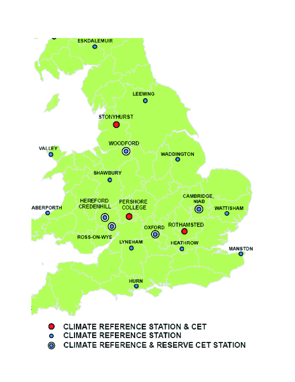
Figure 1: Excerpt of Great Britain’s map with climate stations locations according to the legend shown in the figure. $\copyright$ Crown 2009, the Met Office (Reproduced with permission.)

The first compilation of a monthly series was presented by Manley manley1953 ; manley1974 covering the years from 1659 to 1973. Afterwards, these data were updated to 1991 when Parker et al. (1992) calculated the daily series. Taking urban warming into account, the same data have been adjusted by 0.1-0.3 Celsius degrees since 1974. From January 1878 until November 2004, the data were recorded by the Met Office using the stations of Rothamsted, Peershore College and Ringway and from the latter date onwards the station of Stonyhurst replaced Ringway. At the same time, revised urban warming and bias adjustments have been introduced in the data registered at Stonyhurst station.

The construction of the CET time series is a five-step procedure. In the two first steps, the daily maximum and minimum temperatures (or the temperature at specific hours) are averaged for specific station and the values from the stations are combined. In the remaining stages, adjustments related to monthly average, variance and urban warming are performed, resulting in a homogeneous times series, as confirmed by previous studies parker2005 ; jones . Further details about each step are described in Parker and Horton (2005)parker2005 , Section 3. The meticulous work in constructing and validating the CET series ensure both the reliability the accuracy of the datajones87 ; zorita .

In the present work, we analyze the daily temperature anomalies, which are the differences between the daily temperatures and the climatological annual cycle of temperature, which is defined, for each day, as the sum of the temperatures of this day carried out over all the years available, divided by its number. The data used in this work have been obtained from KNMI (The Royal Netherlands Meteorological Institute) Climate Explorer website http://climexp.knmi.nl/. The annual moving average of the CET anomaly time series is presented in Fig. 2.

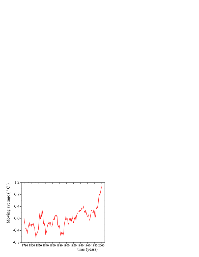
Figure 2: Daily temperature anomaly averaged over a $11$-year sliding window (step size of one year) for the Central England Temperature (CET) time series.

In performing this study, we follow a twofold approach: first, we analyze the overall self-similar characteristics of the CET anomaly and then we focus on the nonstationarities of the time series. In both cases we employ the same quantitative tools. Specifically, in the latter approach we scan the daily time series, from $1772$ to $2007$, using a $11$-year sliding window. Each window starts on the $1st$ January of year $i$ and ends on the $31st$ December of the year $i+10$, resulting in window of $11\times 365$ points. If $N$ is the number of years in the series, there will be $N-10$ ($=226$) windows, the centers of which are located at the year $i+5$, resulting in a step size of one year. We have chosen to use $11$-years sliding windows because: a) it contains more than $4000$ data points in each window, which is enough for a sufficiently accurate estimation of a multifractal spectrum serrano ; b) it produces a sufficient number of windows for an appropriate assessment of the evolution of the scaling properties of the system (the larger the windows, the smaller their number); c) it does not affect our spectra and thus our results since no time scale multiple of $11-$years was found in the spectrum analysis; d) in using overlapping instead of nonoverlapping windows we are able to detect significant changes that otherwise would have passed unnoticed.

II.2 Methods

II.2.1 Multifractal detrended fluctuation analysis - MF-DFA

Methods of scaling analysis, such as the Detrended Fluctuation Analysis (DFA) have already been used in other climate studies kurnaz . Particularly, this method has been employed in the study of the evolution of the Hurst exponent of temperature time series alvarez . The DFA quantifies the relation between the variance of the accumulated sum of the signal and the size of the interval considered in the sum. Before computing the variance as a function of this time interval a detrending procedure, which seeks to remove pre-existing nonstationarities, is applied to the signal. The DFA equally weighs large and small deviations and is thus unable to provide any information about the influence of their magnitudes. The method can be modified to check whether there exists an unequal contribution of large and small variations in the scaling behavior of a time series. This generalization is called multifractal detrended fluctuation analysis (MF-DFA) mf-dfa .

The MF-DFA is one of the most applied methods to determine the multi-scaling features of a time series mf-dfa-appl1 ; mf-dfa-appl2 ; mf_dfa_appl3 ; mf-dfa-appl4 ; canberra ; zhou-chem ; zhou-fin . We have opted to apply the MF-DFA rather than employ the Wavelet Transform Modulus Maxima (WTMM) wavelet because the WTMM is prone to introduce artificial multifractality in a higher degree polacos . Additionally, MF-DFA gives better results for short signals polacos .

Considering a time series $\left\{x\left(i\right)\right\}$ ($x$ represents the temperature anomaly in our case) composed of $N$ elements, the MF-DFA consists of the following steps:

• Determine the profile $Y\left(i\right)$ of the cumulative deviation of the elements from the mean

  $$Y\left(i\right)=\sum_{l=1}^{i}\left[x\left(l\right)-\left\langle x\right\rangle\right],$$ (2)

  where $\left\langle\ldots\right\rangle$ represents the average over elements and $i=1,...,N$.

• Divide the new profile $Y\left(i\right)$ into $N_{s}\equiv\mathrm{int}\left(\frac{N}{s}\right)$ nonoverlapping intervals of equal size $s$.

• Compute the trend of each interval by a least-squares adjustment method, and from that the variance for each segment $\nu=1,\ldots,N_{s}$.

  $$F^{2}\left(\nu,s\right)=\frac{1}{s}\sum_{l=1}^{s}\left\{Y\left[\left(\nu-1\right)\,s+l\right]-y_{\nu}\left(l\right)\right\}^{2},$$ (3)

  where $y_{\nu}\left(l\right)$ represents a $p^{th}$-order fitting polynomial in the segment $\nu$. The value of $p$ might be relevant to the results. For the CET anomaly time series we used polynomials of $2^{nd}$-order, because using higher order polynomials does not significantly affect the multifractal spectrum.

• Determine the fluctuation function of order $z$, $F_{z}\left(s\right)$ given by

  $$F_{z}\left(s\right)\equiv\left\{\frac{1}{N_{s}}\sum_{\nu=1}^{N_{s}}\left[F^{2}\left(\nu,s\right)\right]^{z/2}\right\}^{1/z},\qquad\forall_{z\neq 0},$$ (4)

  and

  $$F_{z}\left(s\right)\equiv\exp\left\{\frac{1}{2N_{s}}\sum_{\nu=1}^{N_{s}}\ln\left[F^{2}\left(\nu,s\right)\right]\right\},\qquad z=0.$$ (5)

  Owing to the fact that the number of points $N$ is not generally a multiple of the scale $s$, the procedure described in the previous item may be also performed on the series with the order of the nonoverlapping segments reversed. In this case, the sum in the fluctuation function (Eqs. 4 and 5) will have twice the number of terms and must be divided by two.

  Equation  (4) presents the basic difference between the DFA and the MF-DFA methods. In the DFA method $z$ has only one value ($z=2$), while in the MF-DFA $z$ can have any real value. Negative values of $z$ decrease the influence of large values of $F^{2}(s)$ on the fluctuation function, whereas positive values of $z$ decrease the influence of small values. The behavior of $F_{z}(s)$ for different values of $z$ reveals the impact of the different scales present in the data.

• Assess the scaling behavior of $F_{z}\left(s\right)$ in $\log-\log$ plots of $F_{z}\left(s\right)$ versus $s$ for each value of z. If the series $\left\{x\left(i\right)\right\}$ shows multiscaling features then,

  $$F_{z}\left(s\right)\sim s^{h\left(z\right)}.$$ (6)

When the exponent $h(z)$ is negative or close to zero (which is not the case in our results), some of equations described in this section must be slightly modified mf-dfa .

If $z<0$, small fluctuations generally lead to large values of $h(z)$, whereas large fluctuations are described by small values of $h(z)$. If $z>0$, the opposite is true.

It is possible to connect the scaling exponent $h(z)$ in Eq. (6), to the scaling exponent $\tau(z)$ of the the partition function in the standard multifractal formalism feder . For multifractal measures this function scales with the size $s$ of the interval as

$$Z_{z}\left(s\right)\sim s^{\tau\left(z\right)}.$$ (7)

Since that the fluctuation function $F_{z}\left(s\right)$ is related to the partition function $Z_{z}\left(s\right)$ by mf-dfa :

$$Z_{z}\left(s\right)\sim s^{-1}\left[F_{z}\left(s\right)\right]^{z},$$ (8)

then, according to Eqs. (7) and (8) we have,

$$\tau\left(z\right)=z\,h\left(z\right)-1.$$ (9)

The Legendre transform of this equation yields,

$$f\left(\alpha\right)=z\,\alpha-\tau\left(z\right),$$ (10)

where is $\alpha$ is exponent mentioned in the Introduction (Eq. 1) and $f(\alpha)$ is the dimension of the subset of the data that is characterized by $\alpha$. mf-dfa

Finally, we can relate the exponent $h\left(z\right)$ to the exponent $\alpha$ by

$$\alpha=h\left(z\right)+z\frac{dh\left(z\right)}{dz},$$ (11)

and

$$f\left(\alpha\right)=z\,\left[\alpha-h\left(z\right)\right]+1.$$ (12)

For $z=2$, $h\left(2\right)\equiv H$ corresponds to the Hurst exponent customarily determined by methods such as the original $R/S$ ratio or the original DFA dfa ; hurst with $H=(\beta+1)/2$, where $\beta$ is the power spectrum exponent we mentioned in the Introduction. Complementary, $z=0$ give us the support dimension of the self-affine structure. In the case of a monofractal, $h\left(z\right)$ is independent of $z$. This implies homogeneity in the scaling behavior and thus Eq. (9) reduces to $\tau\left(z\right)=z\,H-1$. Explicitly, there are only different values of $h\left(z\right)$ if large and small fluctuations scale differently. Lastly, we must stress we are not using the term fractal in absolutely formal way. In fact, although in some cases $h(z)$ matches the box-counting dimension, this exponent generally does not verify all the properties of the Hausdorff-Besicovitch dimension of a signal. For further details on this subject the reader is pointed to Ref. feder, .

II.2.2 Components of multifractality

There are two ingredients that introduce multifractality in a time series: deviations from a scale dependent distribution and dependence between the measurements that compose the time series. These factors are traditionally assumed as independent and thus the total multifractality usually stems from the superposition of both. This means we can attribute a certain value $h_{\mathrm{NG}}(z)$ to the non-Gaussianity and the difference $h(z)-h_{\mathrm{NG}}(z)$ to the dependence between measurements note1 However, we must remember that this is not entirely true. For instance, processes with time-dependent standard deviation such as ARCH-like  proposals (the so-called heteroscedastic models), the two elements of multifractality are strongly dependent because the non-Gaussianity of the time series originates from the existence of dependencies between elements that are linearly dependent in the local variance (or squared volatility in financial jargon), tough the variable is itself uncorrelated archmodels . When the dependence in the volatility is set to zero, the outcome is a Gaussian series and the two contributions to multifractality are one and the same. From Eqs. (9)-(12), we can see that a straightforward way of assessing the existence of multifractal features is to compute the difference, $\Delta\alpha$, between the minimum and the maximum values of the spectrum $f(\alpha)$. If the series is a mono-fractal we have $\Delta\alpha=0$, or else we should be able to separate the contributions due to non-Gaussianity, $\Delta\alpha_{\mathrm{NG}}$, and to the linear, $\Delta\alpha_{\mathrm{LD}}$, and the nonlinear dependencies, $\Delta\alpha_{\mathrm{NL}}$, so that,

$$\Delta\alpha=\Delta\alpha_{\mathrm{NG}}+\Delta\alpha_{\mathrm{LD}}+\Delta\alpha_{\mathrm{NL}}.$$ (13)

It is often assumed that linearities do not contribute to the multifractal width because they are traditionally related to a single scale of dependence. However, previous results on financial data jef-csf ; zhou-fin have shown that these linear/weak dependencies do modify the MF-DFA spectrum. Therefore, we shall not omit its contribution a priori. Let us consider that the time series $\left\{x\left(i\right)\right\}$ has a non-Gaussian distribution and dependence between elements. In performing an appropriate shuffling process, we are defining a new series with the same probability density function as the original signal, but for which there is no dependence between the elements, because the memory was totally destroyed. As proven in Ref. mf-dfa, , when we analyze the multifractal spectrum of the shuffled surrogate, it will differ from the mono-fractal behavior, $\Delta\alpha=\Delta\alpha_{\mathrm{(shuf)}}\neq 0$, only due to the non-Gaussianity of the probability density function and thus,

$$\Delta\alpha_{\mathrm{NG}}=\Delta\alpha^{\mathrm{eff}}_{\mathrm{(shuf)}},$$ (14)

where $\Delta\alpha^{\mathrm{eff}}$ is the effective $\Delta\alpha$ that will be defined in the next paragraph. On the other hand, we can apply a procedure of phase randomization in which we Fourier transform the series in the frequency domain $\omega$ and replace the phases with uniformly distributed random values up to the first half of the transformed series (excluding the phases of $\omega=-\pi,0$) and complete the surrogate series we use their conjugate values in the remaining of the series. Afterwards, we Inverse Fourier transform the surrogate. The final result is a time series in which the previously existing deviations from the Gaussian has been destroyed (see an example in Fig. 3). Nonetheless, we can verify that the power spectrum of the surrogate is the same as the original series, because we simply changed the phases of the Fourier Transform of the time series whilst preserving its absolutes values. Since the power spectrum describes the linear dependencies (or correlations), when we evaluate the multifractality of the new series, $\Delta\alpha_{\mathrm{(rand)}}$, the only contribution originates in the linearities of the system,

$$\Delta\alpha_{\mathrm{LD}}=\Delta\alpha_{\mathrm{(rand)}}^{\mathrm{eff}}.$$ (15)

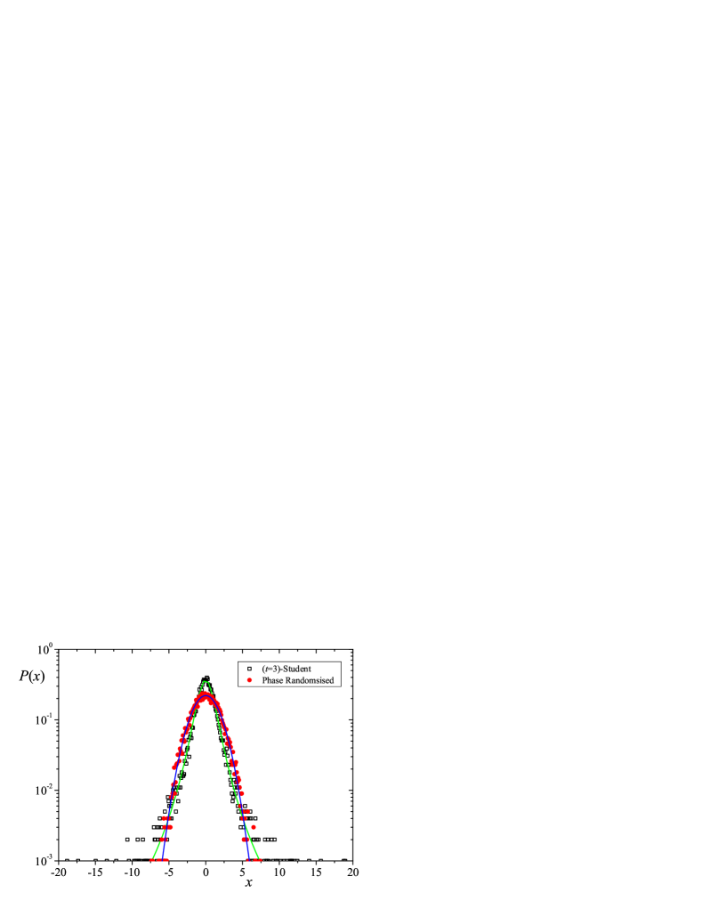
Figure 3: (Color online) The $(\square)$ symbols were obtained from a series of $10^{4}$ elements following a ($t=3)$-Student distribution (or a $(q=3/2)$-Gaussian with $\sigma^{2}=3$) which was shuffled in order to remove any possible dependence between the variables due to the pseudo-random generator gentle and the $(\bullet)$ symbols represent the Gaussian of the surrogate time series that is obtained by the phase randomization procedure.

When we analyze the multifractal nature of a series that was both shuffled and phase randomized (or vice-versa) we are expected to get $\Delta\alpha_{\mathrm{(shuf\&rand)}}=0$. However, in practice, $\Delta\alpha_{\mathrm{(shuf\&rand)}}\neq 0$. These values different from zero (considering the error bars) are important as they can be used to check the effect of the error introduced by the finiteness of the time series and the method. This allows us to define the effective $\Delta\alpha^{\mathrm{eff}}$ as,

$$\Delta\alpha^{\mathrm{eff}}_{(\ldots)}=\Delta\alpha_{(\dots)}-\Delta\alpha_{\mathrm{(shuf\&rand)}},$$ (16)

for the original, shuffled and random phase time series.

In addition, we assess the joint contributions of the non-Gaussianity and the nonlinearities proceeding in the following way: instead of randomizing the phases of the Fourier Transform ${\tilde{x}(\omega)}$, we preserve them and assign a constant value to the absolute value of $\tilde{x}(\omega)$ keeping in mind that $|\tilde{x}(\omega)|=|\tilde{x}(-\omega)|.$ Acting in this way, we define a new surrogate of the noise with a constant power spectrum, which is typical of a white noise, and with the remaining dynamical features equal to the original signal because of the preservation of the phase. After Inverse Fourier transforming, we compute the multifractal width $\Delta\alpha_{\mathrm{PP}}$, the effective value of which is to be compared with the sum of $\Delta\alpha_{\mathrm{NG}}$ and $\Delta\alpha_{\mathrm{NL}}$.

In spite of the fact that the effect of time dependencies in the multifractality is already taken into consideration in the MF-DFA procedure (D stands for detrended), it is worth mentioning that in order to apply the Wiener-Khinchin relation the series must be stationary or at least close to it. With the purpose to overcome the problem of the nonstationarity of the time series for a proper evaluation of $S(\omega)$, which is only necessary to generate the surrogate series, we have applied a high-pass filter  highpass to remover eventual nonstationarities (frequencies lower than $1/N$). Moreover, we have also used the Burg algorithm  burg1 ; burg2 for estimating $S(\omega)$ since it is very difficult to distinguish noise from information in the standard FFT spectrum. Nevertheless, we can still ask the following question: what are the actual advantages of a multifractal study? Simple systems are traditionally characterized by the existence of a typical scale that implies an exponential dependence of quantities such as distribution, correlation and relaxation. For more complex systems, which are governed by nonlinear mechanisms, the existence of a typical scale is replaced with scale invariance relations that are depicted by power laws as that of Eq. (1). Therefore, when the system is “weakly” complex the data are described by a single exponent and the multifractal width vanishes. On the other hand, when the system is complex altogether, we have a series of power-law exponents defining the system and thus the multifractal width is different from zero. In other words, the larger $\Delta\alpha$, the more complex the system.

III Results

III.1 Overall results

In this sub-section, we first analyze the time series as a single set. The scaling law (Eq. 6) is verified in the range $s=27$ to approximately $s=16000$ days. The results of the multifractal analysis of the CET anomaly time series and its various surrogates described in the previous section are depicted in Fig. 4. For all the curves we verify the fat-fractal nature of the series as the maximum of $f(\alpha)$ is equal to 1. In extrapolating the values $\alpha_{\mathrm{min}}$ and $\alpha_{\mathrm{max}}$ at which the $f(\alpha)$ curve intersects the $\alpha$ axis, we determined for the original time series that $\Delta\alpha=0.38$. For the shuffled plus randomized surrogate we obtained $\Delta\alpha_{(\mathrm{shuf\&rand)}}=0.16$ yielding an effective width $\Delta\alpha^{\mathrm{eff}}=0.22$. Concerning the remaining surrogates we got the following effective values $\Delta\alpha_{(\mathrm{shuf)}}^{\mathrm{eff}}=\Delta\alpha_{\mathrm{NG}}=0.02$, $\Delta\alpha_{(\mathrm{rand)}}^{\mathrm{eff}}=\Delta\alpha_{\mathrm{LD}}=0.14$ and $\Delta\alpha_{\mathrm{NL}}=0.06$. On the other hand, the computation of the multifractal width of the phase-preserved surrogate yielded $\Delta\alpha_{(\mathrm{PP)}}=0.06$. Taking into account the error ($\pm 0.01$ in our analyses) the relation,

$$\Delta\alpha_{\mathrm{PP}}\simeq\Delta\alpha_{\mathrm{NL}}+\Delta\alpha_{\mathrm{NG}},$$ (17)

is verified.

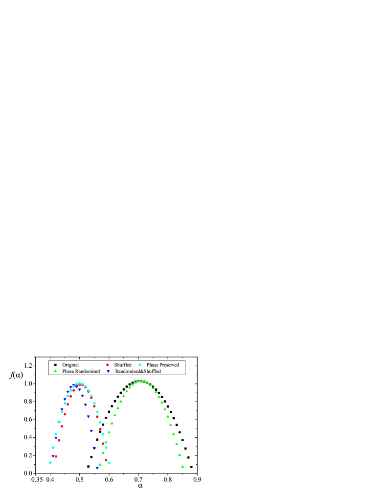
Figure 4: (Color online) Multifractal spectrum $f(\alpha)$ vs $\alpha$ for the original CET anomaly and for the surrogates generated by shuffling, phase randomizing, shuffling plus phase randomizing and phase preservation.

The small contribution of the non-Gaussianity to the overall multifractal width is easily understandable allowing for the quasi-Gaussian form of the CET anomaly probability density function.

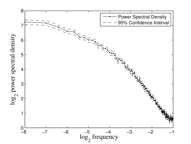
Figure 5: (Color online) Power spectrum $S(\omega)$ vs $\omega$ for the CET anomaly obtained using the Burg algorithm. burg1 ; burg2 The dashed lines represent the error margins ( 5 % of the power spectrum value).

These results, particularly the influence of the linear correlations can be double-checked. Explicitly, we can define a new surrogate which retains the power spectrum $S\left(\omega\right)$ (shown in Fig. 5) of the CET anomaly but whose elements have a Normal distribution and only exhibit linear dependencies between them. This is achieved by first generating a series composed of a sequence independent and identically normally distributed random variables that is, then, Fourier transformed. The amplitude of each element in the set $\left\{\tilde{x}\left(\omega\right)\right\}$ is modified by multiplying it by $\sqrt{S\left(\omega\right)}$. Thereafter, we apply the inverse Fourier transform. The results of this procedure are depicted in Fig. 6, which shows an effective width $\Delta\alpha_{(\mathrm{fourier)}}^{\mathrm{eff}}=0.15$, completely compatible with the result $\Delta\alpha_{\mathrm{LD}}$ presented before.

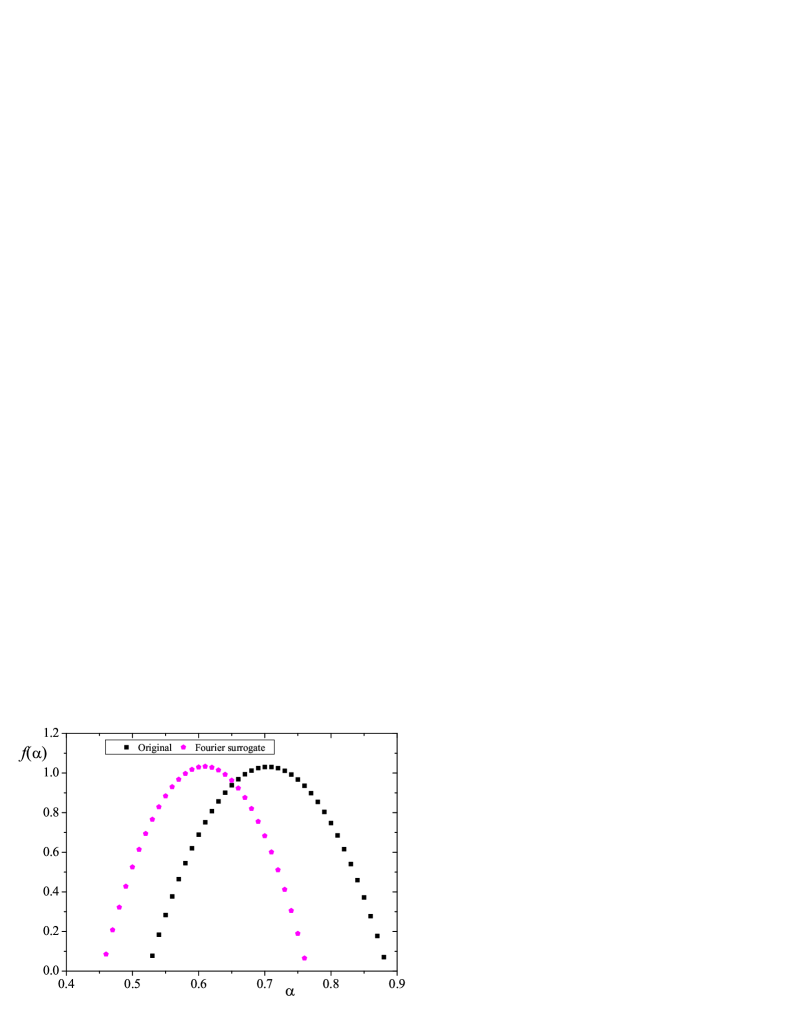
Figure 6: (Color online) Multifractal spectrum $f(\alpha)$ vs $\alpha$ for the original CET anomaly and for the surrogate in which the power spectrum is kept. In spite of being shifted one another, it is visible that the width of both spectra is are very similar. Moreover, the multifractal width $\Delta\alpha_{(\mathrm{Fourier)}}$ lies within $\Delta\alpha_{(\mathrm{rand)}}$.

III.2 Time dependence of the components of multifractality

We now present the results obtained with 11-year sliding windows which allow us to describe the dynamical features of multifractalitity in the CET anomaly. The multifractal spectrum has been fitted in range $16-1024$ days. Fig. 7 shows how the multifractality has changed in time. This multifractal dynamics can be fine-tuned by obtaining the effective multifractal width $\Delta\alpha^{\mathrm{eff}}$. The results of this refining are striking. On average, the effective multifractality represents just about $50\%$ of the width obtained from the original CET anomaly time series in Fig. 7. Concerning the elements of multifractality, we can use Eq. (14) and Eq. (15). Analyzing the contribution of non-Gaussianity (Fig. 8), $\Delta\alpha_{NG}$, we see that only $33$ out of the $226$ values of $\Delta\alpha^{\mathrm{eff}}_{(shuf)}$ are actually different from zero and consequently from a single-structure nature. This implies an average contribution of merely 3%, which once again is in accordance with the quasi-Gaussian nature of the time series. The contribution linear dependencies, $\Delta\alpha_{LD}$, which is obtained when we convert our series into a Gaussian series by means of the phase randomization procedure, is of 59% (Fig. 8). Adding the two contributions we do not get 100 %. This implies that the multifractality introduced by nonlinearities corresponds to an average of 38% (Fig. 9).

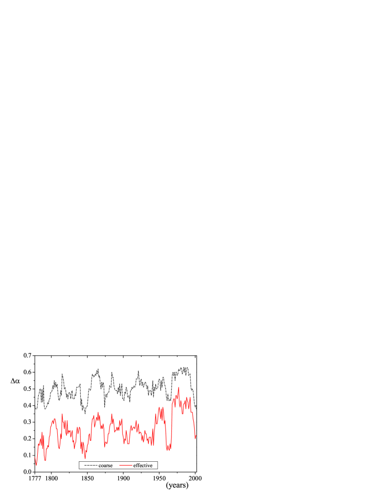
Figure 7: (Color online) Multifractal width $\Delta\alpha$ of the Central England temperature anomaly between 1777 and 2002, coarse and effective. The $\Delta\alpha^{eff}$ is obtained after removing finite size effects and systematic algorithmic error, by subtracting from the original $\Delta\alpha$, the value of $\Delta\alpha_{(shuf\&rand)}$ as described in Eq. (16). Each curve follows the legend in the figure.

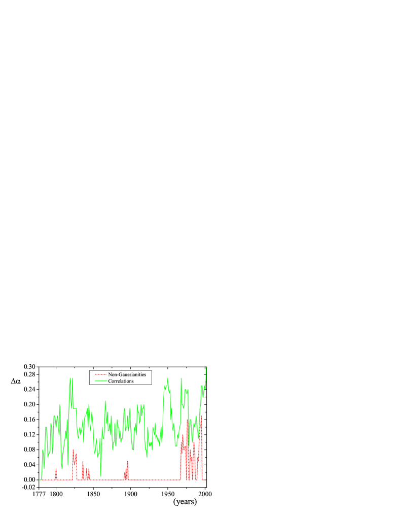
Figure 8: (Color online) non-Gaussian and linear dependence (correlations) contributions to the effective multifractal width $\Delta\alpha^{\mathrm{eff}}$ of the Central England temperature anomaly between $1777$ and $2002$. Each curve follows the legend in the figure. The non-Gaussian character is related to the width of the multifractal spectrum of the shuffled time series, while the linear dependence is related to the width of the multifractal spectrum of the randomized time series. All the calculations have been performed using the effective $\Delta\alpha$ given by Eq. (16).

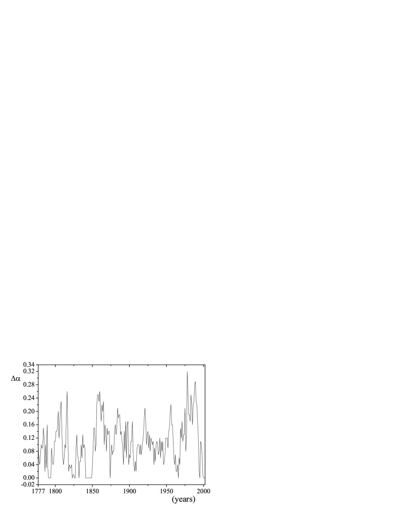
Figure 9: (Color online) Nonlinear dependence contribution to the effective multifractal width $\Delta\alpha^{\mathrm{eff}}$ of the Central England temperature anomaly between 1777 and 2002. This contribution is measured by the width of the $f(\alpha)$ curve of the surrogate time series with the same Fourier spectrum of the original one, but without linear dependence. All the calculations have been performed using the effective $\Delta\alpha$ given by Eq. (16).

III.3 Detecting changes in climate

The results we have presented in the previous sub-section can be compared with the results published by Berkes et al. royal . Using on Functional Data Analysis (FDA), Berkes et al. pointed out a set of statistically significant climate changes in the years of 1780, 1815, 1926 and 2007. Using a different method that the same authors named MDA, the climate changes occurred in 1780, 1808, 1850, 1926, 1992 and 2007. Our results, show changes in the non-Gaussianity around 1800, followed by the flurried periods 1820-1829, 1834-1845, 1891-1897 and a last and standing disturbed period from 1966 on (Fig. 8). Although Berkes et al.royal analyzed climate variations by measuring quantities different from the multifractal characteristics determined here, changes in the dynamics of a given observable can be identified using very different quantities the variations of which are related to the dynamics of this observable. Therefore, it is legitimate to consider this concurrence indicative of the robustness of past changes in the leading dynamical mechanism of the temperature anomaly. Although we could not observe any change in 1926 or thereabouts in Fig. 8, we noticed that there is a sharp peak close to this date in Fig. 9. It is worth emphasizing that Berkes et al. royal to their methods, especially the latest one, as a “mere modeling assumption that is useful in identifying patterns of change in mean temperature curves”. Furthermore, we perceive that the broader and larger nonlinear and non-Gaussian contributions to overall multifractality start in the mid 1960s and persist until the late 1990s. A pattern of successive positive values in the annual average of the CET anomaly was reported by Parker et al. (1992) in this period parker1992 and encloses a global change of phase that is well-documented in the climate literature ipcc . Last but not least, we have observed that the peaks verified in the $\Delta\alpha_{\mathrm{NG}}$ (Fig. 8) concur with the emergence of kurtosis excess when statistical moments are surveyed aguasdelindoia . Recently, results by Hansen et al.hansen in a global climate change study using a standard statistical approach indicated that the temperature anomaly in the last decades exhibits non-Gaussian distributions. Motivated by the time dependence of the scaling properties of the CET anomaly, we analyzed the spectra $\alpha_{\mathrm{min}}$ and $\alpha_{\mathrm{max}}$ (effective values) (Fig. 10). The maxima in the amplitude of both spectra agree with decadal oscillations. Namely, we found for $\alpha_{\mathrm{min}}$ maxima at $16^{-1}$ and $32^{-1}$ year^-1 and for $\alpha_{\mathrm{max}}$ maxima at $17^{-1}$, $34^{-1}$ year^-1 with the former having an extra peak at $55^{-1}$ year^-1. These decadal oscillations are not present when the width $\Delta\alpha$ is analyzed. One reason for that stems from the fact that both $\alpha_{\mathrm{max}}$ and $\alpha_{\mathrm{min}}$ show very close peaks in the spectrum and thus when the difference between them is considered the peaks are not perceived, which is similar to what occurs with two co-evolving quantities.

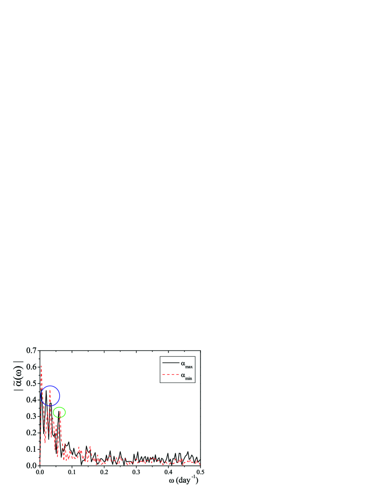
Figure 10: (Color online) Amplitude of Fourier transform ($\tilde{\alpha}(\omega)$) of the maximum and the minimum values of $\alpha(t)$, against frequency. The circles identify the local maxima described in the text.

IV Final remarks and outlook

In this manuscript we studied the multifractal features of the CET anomaly. This was carried out by considering the entire time series and by scanning the time series with 11-year sliding windows. Our results show that the main component of the multifractal structure of this time series is due to the linear dependencies in the dynamics, followed by nonlinear dependencies and with a residual contribution of the deviations from the Gaussianity. Nonetheless, when we analyzed how the multifractality of the CET anomaly changes in time, we verified that until 1950 the non-Gaussian contribution appears in dates that are very close to the dates associated with climate changes, as presented in a previous study using Functional Data Analysis royal . From the 1960s onwards the contribution of the non-Gaussianity becomes significant for most of the time, a result that matches a recent finding of temperature anomalies significantly beyond the $3\,\sigma$ criterion that characterizes the invalidity of the Gaussian hansen .

Finally, although the scope of the present work concerns the quantitative description of the multifractal properties of the CET anomaly, our analysis can have direct implications in modeling as well. Our results indicate that the temperature variability modeling must take into account the multifractal nature of the temperature time series, and also the contribution of each ingredient for the multifractality. A tentative dynamical scenario is that wherein we resort to the statistical mechanics relation between temperature and standard deviation, i.e., the temperature is proportional to the standard deviation, and consider a model inspired in cascade models of the latter quantity for turbulent fluids such as those introduced in Refs. meneveau, ; castaing, ; arneodo, . Instead of considering a cascade process in the standard deviation of the quantity under analysis, we reinterpret those models considering a cascade process for the average value of the observable, which in this case is the temperature anomaly. In this approach, the average value over a certain scale $\ell$ comes from the multiplicative process,

$$\mu_{\ell}\left(t\right)=\prod\limits_{i=0}^{n-1}f\left(i\rightarrow i+1\right)\,\mu_{L},$$ (18)

with $\mu_{L}$ representing the average over a reference period $L$, e.g. $L=11$ years, and $f$ representing the fraction of measure (average) passing from a earlier generation (time scale) to the subsequent. In this case, the greater $i$, the smaller $\ell$, i.e., $i=0$ corresponds to $\ell=L$ and $\ell=n$ yields the scale of the temperature anomaly we are intend to describe. Consequently, the temperature anomaly, $\xi$, would be equal to,

$$\xi_{\ell}\left(t\right)=\varepsilon\left(t\right)+\mu_{\ell}\left(t\right),$$ (19)

where $\varepsilon$ represents a Gaussian independent and identically distributed noise with zero average and appropriate standard deviation. A skew distribution of $\mu_{L}$ will lead to a skew distribution of $\xi$ as well. Concomitantly, in order to represent the slight kurtosis we can consider a further contribution, $\zeta$, coming from a multiplicative noise process,

$$\zeta\left(t\right)=\eta\left(t\right)\,\sigma\left(t\right)\,h\left(t\right),$$ (20)

with $\sigma\left(t\right)$ being a function of past values of $\xi$ and $\zeta$ in a heteroscedastic way (see for details garch, ; andersen, ) and $\eta$ another Gaussian noise not correlated with $\varepsilon$. The $\zeta$ contribution is modulated by a step function $h\left(t\right)=\Theta\left[t-\left(\Upsilon-\Delta\Upsilon\right)\right]\Theta\left[\Upsilon+\Delta\Upsilon-t\right]$ where the center of the intervals come from a shot noise following a frequency related to Fig. (10), i.e., a random process that has nonzero values at an average rate, $\lambda$, which belong to the Poisson class of stochastic processes. Mathematically, the probability of having a contribution from $\zeta$ arising from a perturbation centered at time $\Upsilon$ is given by,

$$p\left(\Upsilon\right)\varpropto\sum\nolimits_{i}\delta\left(\Upsilon-\Upsilon_{i}\right)\,,$$ (21)

and the total temperature anomaly will thus correspond to the sum of $\xi_{\ell}\left(t\right)$ and $\zeta\left(t\right)$.

Alternative models can be presented, namely for mimicking the fluctuations of the temperature anomaly instead of the temperature itself. It is simple to find one quantity after the other bearing in mind their relation and statistical properties as in happens in other problems such as fluid turbulence and price dynamics in financial markets.

One the other hand, still in the context of the empirical analysis, the present study can be further expanded into the statistical and dynamical analysis of yearly $\Delta\alpha$ fluctuations, especially its probability density function and the existence of a mixture dynamical regimes by the application of nonparametric testing dks .

IV.0.1 Acknowledgements

We would like to thank the Met Office for kindly providing us with the map in Fig. 1. AMG has received funding from CNPq (Brazilian National Council for Scientific and Technological Development), and from the EU Seventh Framework Programme (FP7/2007-2013) under Grant Agreement nr 212492 (CLARIS LPB. A Europe-South America Network for Climate Change Assessment and Impact Studies in La Plata Basin). JdS acknowledges CNPq, PETROBRAS$/$FUNPAR-UFPR, Setor de Ciências Exatas - UFPR and Setor de Ciências da Terra - UFPR for support and S. H. S. Schwab, F. Mancini, F. J. F. Ferreira, are also thanked for valuable helping and encouragement. SMDQ thanks the LABAP laboratory of Universidade Federal do Paraná for the warm hospitality during his visits to the institution sponsored by CNPq and PETROBRAS$/$FUNPAR-UFPR and the European Commission through the Marie Curie Actions FP7-PEOPLE-2009-IEF (contract nr 250589).

References

- (1) Mandelbrot BB (1982), The Fractal Geometry of Nature. W. H. Freeman and Co., New York.
- (2) Mandelbrot BB (1999) Multifractals and 1/ Noise. Springer, New York.
- (3) Schertzer D. and Lovejoy S. (eds.) (1991) Scaling, Fractals and nonlinear Variability in Geophysics. Kluwer, Boston.
- (4) Falconer K (1990) Fractal Geometry: Mathematical Foundations and Applications. Wiley, New York.
- (5) Kurnaz ML (2004) Detrended fluctuation analysis as a statistical tool to monitor the climate. J. Stat. Mech. P07009
- (6) Alvarez-Ramirez J, Alvarez J, Dagdug L, Rodriguez E, Carlos Echeverria J (2008) Long-term memory dynamics of continental and oceanic monthly temperatures in the recent 125 years. Physica A: Statistical Mechanics and its Applications 387(14):3629-3640.
- (7) Ashkenazy Y, Baker DR, Gildor H, Havlin S (2003) Nonlinearity and multifractality of climate change in the past 420,000 years. Geophys Res Lett 30:2146.
- (8) Bodri L and Cermak V (2005) Multifractal analysis of temperature time series: data from boreholes in Kamchatka. Fractals 13 299.
- (9) Karimova L, Kuandykov Y, Makarenko N, Novak MM and Helama S (2007) Fractal and topological dynamics for the analysis of paleoclimatic records. Physica A 373 737.
- (10) Oñate Rubalcaba JJ (1997) Fractal analysis of climatic data: Annual precipitation records in Spain. Theoretical and Applied Climatology 56 83.
- (11) Valencia JL, Saa Requejo A, Gascó JM and Tarquis AM (2010) A universal multifractal description applied to precipitation patterns of the Ebro River Basin, Spain. Clim. Res. 44 17.
- (12) Dyer TGJ (1976) An analysis of Manley’s central England temperature data: I. Q.J.R. Meteorol. Soc. 102(434), 871 888.
- (13) Bain WC (1976) The power spectrum of temperatures in central England. Q.J.R. Meteorol. Soc. 102(432), 464 466.
- (14) Lovejoy S and Schertzer D (1986) Scale invariance in climatological temperatures and the spectral plateau. Annales Geophys. 4B, 401-410.
- (15) Matyasovszky I (1989) Further results of the analysis of central England temperature data. Theoretical and Applied Climatology. 39(3), 126-136
- (16) Pelletier JD (1998) The power spectral density of atmospheric temperature from time scales of 10 to 10?6 yr. Earth and Planetary Science Letters. 158 157 164
- (17) Harvey DI Mills TC 2003 Modelling Trends in Central England Temperatures. Journal of Forecasting 22:35-47.
- (18) Hannachi A 2006 Quantifying changes and their uncertainties in probability distribution of climate variables using robust statistics. Climate Dynamics 27(2-3):301-317.
- (19) Kwon H-H,Lall U, Khalil AF (2007) Stochastic simulation model for nonstationary time series using an autoregressive wavelet decomposition: Applications to rainfall and temperature. Water Resources Research 43:W05407.
- (20) Zhang T Wu WB 2011 Testing parametric assumptions of trends of a nonstationary time series. Biometrika 98(3):599-614.
- (21) Zhang X and Shao X 2011 Testing the structural stability of temporally dependent functional observations and application to climate projections. Electronic Journal of Statistics 5:1765-1796.
- (22) Franzke C 2012 Nonlinear Trends, Long-Range Dependence, and Climate Noise Properties of Surface Temperature. J. Climate 25:4172-4183.
- (23) Manley G (1953) The mean temperature of central England, 1698-1952. Quarterly Journal of the Royal Meteorological Society 79(340):242-261.
- (24) Manley G (1974) Central England temperatures: monthly means 1659 to 1973. Quarterly Journal of the Royal Meteorological Society 100(425): 389-405.
- (25) Parker DE, Legg TP, Folland CK (1992) A new daily Central England Temperature series 1772-1991. Int. J. Clim. 12:317.
- (26) Parker DE, Horton EB (2005) Uncertainties in central England temperature 1878-2003 and some improvements to the maximum and minimum series. Int. J. Climatology 25:1173-1188.
- (27) Probert-Jones JR (1984) On the homogeneity of the annual temperature of central England since 1659. International Journal of Climatology 4 241.
- (28) Jones DE 1987 Daily Central England Temperature: recently constructed series. Weather 42(5) 130-133.
- (29) Zorita E Moberg A Leijonhufvud L Wilson R Brázdil R Dobrovolný P Luterbacher J Böhm R Pfister C Riemann D Glaser R Söderberg J González-Rouco F 2010 European temperature records of the past five centuries based on documentaryinstrumental information compared to climate simulations. Climatic Change 101:143-168.
- (30) Serrano E and Figliola A (2009), Wavelet Leaders: A new method to estimate the multifractal singularity spectra. Physica A, 388 2793-2805.
- (31) Kantelhardt JW, Zschiegner SA, Koscielny-Bunde E, Havlin S, Bunde A, and Stanley HE (2002) Multifractal detrended fluctuation analysis of nonstationary times series. Physica A 316:87-114.
- (32) Ivanov PCh, Amaral LAN, Goldberger AL, Havlin S, Rosenblum MG, Stanley HG, Struzik ZR (1991) From 1/f noise to multifractal cascades in heartbeat dynamics. Chaos 11:641-652.
- (33) Matia K, Ashkenazy Y, Stanley HE (2003) Multifractal properties of price fluctuations of stocks and commodities. Europhys Lett 61:422-428.
- (34) Telesca L, Lapenna V, Macchiato M (2005) Multifractal fluctuations in earthquake-related geoelectrical signals. New J Phys 7:214.
- (35) Duarte Queirós SM, Moyano LG, de Souza S, Tsallis C (2007) A nonextensive approach to the dynamics of financial observables. Eur Phys JB 55:161-167.
- (36) Niu M-R, Zhou W-X, Yan Z-Y, Guo Q-H, Liang Q-F, Wang F-C, Yu Z-H (2008) Multifractal detrended fluctuation analysis of combustion flames in four-burner impinging entrained-flow gasifier. Chem Eng J 143:230.
- (37) Zhou W-X (2009) The components of empirical multifractality in financial returns. EPL 88:28004; Zhou W-X (2012) Finite-size effect and the components of multifractality in financial volatility. Chaos, Solitons & Fractals 45:147
- (38) Ausloos M (2012) Generalized Hurst exponent and multifractal function of original and translated texts mapped into frequency and length time series. Phys. Rev. E 86 031108
- (39) Muzy JF, Bacry E, Arneodo A. (1991) Wavelets and multifractal formalism for singular signals: Application to turbulence data. Phys. Rev. Lett. 1991;67:3515-3518.
- (40) Oświȩcimka P, Kwapień J, Drożdż S (2006) Wavelet versus detrended fluctuation analysis of multifractal structures. Phys Rev E 74:016103.
- (41) Feder J (1988) Fractals. Plenum, New York.
- (42) Peng C-K, Buldyrev SV, Havlin S, Simons M, Stanley HE, Goldberger AL (1994) Mosaic organization of DNA nucleotides. Phys Rev E 49:1685-1689.
- (43) Hurst HE (1951) Long-term storage capacity of reservoirs. Trans Am Soc Civ Eng 116:770-808.
- (44) Throughout the text we employ the term non-Gaussian in the broad sense, i.e., we use it to refer to a distribution that does not have a defined scale as the Gaussian and which is a established terminology for the absence of scale.
- (45) Gourieroux C and Montfort (1996) A Statistics and Econometric Models. Cambridge: Cambridge University Press.
- (46) de Souza S and Duarte Queirós SM (2007) Effective multifractal features of high-frequency price fluctuations time series and l-variability diagrams. Chaos, Solitons & Fractals 42:2512?2521
- (47) Gentle JE (1995) Random Number Generation and Monte Carlo Methods, 2nd ed. Wiley, New York.
- (48) Paarmann LD (2001) Design and Analysis of Analog Filters - A Signal Processing Perspective. Kluwer, Dordrecht.
- (49) Marple SL (1987) Digital Spectral Analysis. Prentice-Hall, Englewood Cliffs - NJ.
- (50) Stoica P and Moses RL (1997) Introduction to Spectral Analysis. Prentice-Hall, Englewood Cliffs - NJ.
- (51) Berkes I, Gabrys R, Horváth L, Kokoszka P (2009) Detecting changes in the mean of functional observations. Journal of the Royal Statistical Society B 71:927-946.
- (52) IPCC 2007 Climate Change 2007 - The Physical Science Basis Contribution of Working Group I to the Fourth Assessment Report of the IPCC. http://www.ipcc.ch
- (53) de Souza J, Duarte Queirós SM and Grimm AM (2008) Time dependence of the multifractal spectrum and other statistical properties of the Central England Temperature time series. XXXI Enconto Nacional de Física da Matéria Condensada. Águas de Lindóia, Brazil.
- (54) J. Hansen, M. Sato and R. Reudy, Proc. Nat. Acad. Sci. USA, DOI:10.1073/pnas.1205276109 (2012)
- (55) Meneveau C and Sreenivasan KR (1987) Simple multifractal cascade model for fully developed turbulence. Phys. Rev. Lett. 59, 1424.
- (56) Castaing B, Gagne Y and Hopfinger EJ (1990) Velocity probability density functions of high Reynolds number turbulence. Physica D 46 177.
- (57) Arneodo A, Muzy JF and Roux SG (1997) Experimental analysis of self-similarity and random cascade processes: application to fully developed turbulence data. J. Phys. II France 7 363.
- (58) Queirós SMD and Tsallis C (2005) On the connection between financial processes with stochatic volatility and nonextensive statistical mechanics. Eur. Phys. J. B S49 139.
- (59) Andersen TG, Bollerslev T, Diebold FX (2010) Parametric and nonparametric volatility measurement. In: Aït-Sahalia Y, ed. Handbook of Financial Econometrics, volume 1, tools and techniques. Elsevier, Amsterdam.
- (60) Camargo S, Duarte Queirós SM, Anteneodo C (2011) Nonparametric testing of nonstationary time series. Phys. Rev. E 84, 046702