The role of the lattice structure in determining the magnon-mediated interactions between charge carriers doped into a magnetically ordered background

Abstract

We use two recently proposed methods to calculate exactly the spectrum of two spin-${1\over 2}$ charge carriers moving in a ferromagnetic background, at zero temperature, for three types of models. By comparing the low-energy states in both the one-carrier and the two-carrier sectors, we analyze whether complex models with multiple sublattices can be accurately described by simpler Hamiltonians, such as one-band models. We find that while this is possible in the one-particle sector, the magnon-mediated interactions which are key to properly describe the two-carrier states of the complex model are not reproduced by the simpler models. We argue that this is true not just for ferromagnetic, but also for antiferromagnetic backgrounds. Our results question the ability of simple one-band models to accurately describe the low-energy physics of cuprate layers.

I Introduction

Many materials under current study, such as cuprates, manganites, pnictides, irridates, etc., have complicated structures with several types of atoms in the basis. Including orbitals for all these atoms in a model Hamiltonian would make it impossibly difficult to solve, besides introducing unreasonably many parameters.

Thus, the first major challenge in studying such materials is to understand what is the minimal model Hamiltonian that properly captures their low-energy properties. (The second major challenge, of course, is to figure how to solve it). Some steps in this process are fairly straightforward. For instance, many of these materials have layered structures, and there are many indications that the interesting physics is hosted by certain layers which are common to all compounds in the family. It is therefore an easy decision to start by modeling one such layer – for example, a CuO₂ layer for cuprates.

Even though this is a significant simplification, the proper minimal model to describe the low-energy properties of one layer is still not obvious. To continue with the CuO₂ example, one could write a model that includes the $3d_{x^{2}-y^{2}}$ orbitals for Cu, which are known to be half-filled in the undoped parent compound, plus the appropriate $2p_{x/y}$ O orbitals. These are filled in the undoped parent compounds, but the cuprates are charge transfer insulatorsZSA and these are the orbitals expected to host the holes introduced by doping. This approach leads to the three-band model of Emery,E3b although for later convenience we prefer to label it here as a two-sublattice model: one for the Cu sites, effectively hosting spins-${1\over 2}$ if double occupancy is forbidden, and one for the O sites, hosting the holes (the charge carriers).

A simpler option is a one-band Hubbard model which describes effective states located on one lattice (at the Cu sites, for CuO₂ layers), or its even simpler counterpart, the $t$-$J$ model, which additionally discards all doubly occupied states and describes carriers in a spin background. Even these simplest possible interacting Hamiltonians, which depend on only one dimensionless parameter ($U/t$ or $J/t$, respectively) are still far from completely understood in the strongly correlated limit, despite a tremendous amount of effort.hub

It is the difficulty to solve such correlated Hamiltonians that explains the drive to simplify the models that we study to the utmost possible. However, it is reasonable to expect that as more and more details are discarded, there is a point beyond which the model no longer contains the physics that we aim to study. Are the Hubbard or $t$-$J$ models already past this point, as far as cuprates are concerned, or do they still contain the low-energy physics of the more complex Emery model?

An affirmative answer to the latter question was given by Zhang and Rice,ZR who also clarified the nature of the states appearing in these one-band models, namely the Zhang-Rice singlets (ZRS). We review their arguments in some detail below; for now it suffices to say that the ZRS is a composite object involving a doping hole occupying a certain linear combination of O orbitals, and which is locked in a singlet with a hole (spin) at a Cu site.

Zhang and Rice’s work on the equivalence between the low-energy properties of the Emery and $t$-$J$ models is based on arguments limited to the one-carrier (one doping hole) sector. Its validity is still not fully settled because of the lack of exact results for these Hamiltonians. Accurate analytical approximations are not available, while conclusions based on numerical work are hampered by the restriction to rather small clusters. Recent results for clusters with 32 CuO₂ unit cells suggest that at least in parts of the Brillouin zone (BZ), the quantum numbers and symmetries of the lowest eigenstate of the Emery model are different from those of its $t$-$J$ counterpart, although the energy dispersion is rather similar.Bayo1

While efforts to understand if the ZRS offers a good description of the quasiparticle are on-going, it is important to note that even if this is proven true, it would still not settle the question whether one-band models give a proper description of the low-energy properties of weakly doped CuO₂ layers. This is because a model Hamiltonian must describe properly not only individual quasiparticles, but also their interactions. This is especially important in cuprates where high-temperature superconductivity appears upon doping. Much of the community believes the pairing to be mediated through magnon exchange,magnons although phonon-mediated pairingphonons and even combined mechanismsitalians are also favored. Clearly, the model Hamiltonian must describe properly the magnon-mediated interactions before one can decide if they are sufficient to facilitate pairing and superconductivity at these rather high temperatures, or whether coupling to additional bosons, e.g. phonons, needs to be considered.

To settle this issue, one must compare the low-energy properties of the two models in the two-carrier sector; the single-carrier sector has no information about interactions. For the Emery and $t$-$J$ models, such a comparison is even more difficult, since finite size effects become more important as the number of holes increases. Recent efforts in this direction were rather inconclusive.Bayo2

Although the discussion so far was focused on cuprates, similar questions appear for other materials. Is it reasonable to ignoreman the ligand O and use models for manganites which only involve Mn $3d$ orbitals? Do the As ions play any rolepnic in the low-energy physics of pnictides? These and many other similar questions have, as a common denominator, the issue of whether one has to use complex models with different ions on different sublattices to properly describe such materials, or whether it suffices to use one-lattice models, possibly based on some composite states which effectively account for the role played by other ions, such as the ligands.

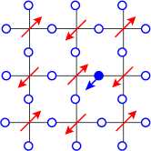
Figure 1: (Color online) Sketch of a CuO₂ plane. If double occupancy is forbidden, each Cu site has a hole in a $3d_{x^{2}-y^{2}}$ orbital, behaving like a spin-${1\over 2}$ (red arrows). Upon doping, the O $2p_{x/y}$ orbitals (empty blue dots) accommodate the doping holes (filled blue dots, with arrows indicating the spins).

Here we focus on one class of such questions, for materials where the parent compound has long range magnetic order and is a charge-transfer insulator. (A short version of this work was published in Ref. old, ). Our conclusions are based on results for the one- and two-carrier sectors for a background that has ferromagnetic (FM) order. This is much simpler than an antiferromagnetic (AFM) background and allows us to find exact solutions, so that we are certain that differences between results are due to the models themselves. We find that the simpler one-lattice models do not properly describe magnon-mediated interactions between carriers, and identify the simple reasons for this. Moreover, we argue that these conclusions are relevant for AFM backgrounds as well. We believe that our results offer strong arguments that the one-band Hubbard and $t-J$ models are inappropriate to describe cuprate layers.

The work is organized as follows. In Section II we briefly review the ZRS arguments. In Section III we introduce our models, which mirror the steps in the ZRS derivation, but for a FM background. Section IV summarizes the formalism (details are presented in various Appendixes). The results are in Section V, and Section VI contains a detailed discussion and our conclusions.

II Brief review of the ZRS

The Emery model for a CuO₂ plane, sketched in Fig. 1, includes explicitly both the Cu and the O sublattices, with their $3d_{x^{2}-y^{2}}$ and $2p_{x/y}$ orbitals, respectively. The goal is to try to reduce it to a one-lattice model, built on effective states located at the Cu sites.

Since the doping hole occupies O $2p$ orbitals, the first step to remove the O sublattice is to make linear combinations of the four O orbitals neighboring one Cu, which are thus centered at the Cu sites $i$. These are described by the $P_{i,\sigma}^{(S,A)}$ operators in Eq. (5) of Ref. E3b, . Because of phase coherence, the “S” combination where the O orbitals have ${x^{2}-y^{2}}$ symmetry is the low-energy state, and from now on we restrict the discussion to it.

The $P_{i,\sigma}^{(S)}$ states are not orthogonal since neighbor Cu share an O ligand, [Eq. (6) of Ref. E3b, ]. To fix this, Zhang and Rice first define their Fourier transforms $P_{\mathbf{k},\sigma}={1\over\sqrt{N_{S}}}\beta_{\mathbf{k}}\sum_{i}e^{-i\mathbf{k}\mathbf{R}_{i}}P^{(S)}_{i,\sigma}$, where the normalization factor $\beta_{\mathbf{k}}=1/\sqrt{1-{1\over 2}(\cos k_{x}+\cos k_{y})}$ is due to the non-orthogonality of the $P^{(S)}_{i,\sigma}$ [Eqs. (8) and (9) of Ref. E3b, ]. It is problematic that $\beta_{\mathbf{k}}$ diverges near the center of the BZ, but ignoring this fact one can Fourier transform back to real space to obtain the operators $\phi_{i,\sigma}={1\over\sqrt{N_{S}}}\sum_{i}e^{i\mathbf{k}\mathbf{R}_{i}}P_{{\mathbf{k}}\sigma}$. These are now properly normalized and describe “effective Cu orbitals”, although they are in fact rather complicated linear combinations of O orbitals. The next step is to note that exchange favors locking a doping hole occupying such an orbital in a singlet with the hole (spin) located on the central Cu. This results in the ZRS described by the operators $\psi_{i}={1\over\sqrt{2}}\left(\phi_{i\uparrow}d_{i\downarrow}-\phi_{i\downarrow}d_{i\uparrow}\right)$, see Eq. (10) of Ref. E3b, . Zhang and Rice then argue that if double occupancy is forbidden, a $t$-$J$ Hamiltonian based on these ZRS captures the low-energy states of the Emery model.

III Models

In an effort to mirror these steps in going from the Emery to the $t$-$J$ model, we study three cases sketched in Fig. 2. For the sake of simplicity we restrict ourselves to one dimension (1D). Generalizations to higher dimensions are straightforward, but as explained below, they do not lead to qualitative changes.

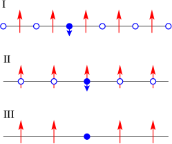
Figure 2: (Clor online) Sketches of the three models. Models I and model II have two bands. One (empty circles) hosts charge carriers introduced by doping (filled circle with arrow for the carrier spin) and the other one hosts lattice spins (red arrows). In model I the carriers propagate on a different sublattice than the one hosting the spins, while in model II, they are on the same lattice. Model III has only one band which hosts both spins (arrows) and ZRS-like objects (filled circle).

Case I is the “parent” two-sublattice, two-band model. One sublattice hosts the lattice spins, of quantum number $S$, while the other hosts the charge carriers. This is the 1D counterpart of the Emery model for the 2D CuO₂ layers if double occupancy is forbidden (apart from the FM order, of course). Model II is a one-lattice, two-band model. One should roughly think of these on-site carrier orbitals as the analogs of the $\phi_{i,\sigma}$ in the ZRS derivation. Finally, model III is an even simpler one-band model, the equivalent of the $t$-$J$ model obtained after locking doping holes in singlets with lattice spins. These parallels will be made more clear in the Results section.

In all these models lattice spins interact ferromagnetically with their nearest neighbors:

$$\mathcal{H}_{S}=-J\sum_{i}(\vec{S}_{i}\vec{S}_{i+1}-S^{2}),$$ (1)

where $\vec{S}_{i}$ is the operator for the spin at site $R_{i}=ia$, and $a=1$ is the lattice constant. Its ground-state is $|{\rm FM}\rangle=|+S,+S,\dots+S\rangle$ and has zero energy. For reasons detailed below, the excited states of interest will be the one-magnon states $S_{q}^{-}|{\rm FM}\rangle=\frac{1}{\sqrt{2SN}}\sum_{i}e^{iqR_{i}}S_{i}^{-}|{\rm FM}\rangle$ with energy $\Omega_{q}=4JS\sin^{2}\left(\frac{q}{2}\right)$. The raising and lowering operators $S_{i}^{\pm}=S_{i}^{x}\pm iS_{i}^{y}$ correspond to creation $(-)$ and annihilation $(+)$ operators for magnons, respectively. If we rewrite $\mathcal{H}_{S}=\mathcal{H}_{S}^{z}+\mathcal{H}_{S}^{x,y}$, where $\mathcal{H}_{S}^{z}=-J\sum_{i}(S_{i}^{z}S_{i+1}^{z}-S^{2})$ and $\mathcal{H}_{S}^{x,y}=-\frac{J}{2}\sum_{i}\left(S_{i}^{+}S_{i+1}^{-}+S_{i}^{-}S_{i+1}^{+}\right)$, it is clear that $\mathcal{H}_{S}^{x,y}$ describes magnon hopping.

In models I and II, the second band hosts spin-$\frac{1}{2}$ charge carriers (electrons or holes) introduced by doping. For model II these carriers propagate on the same lattice as the spins. For model I, they move on a different sublattice which is interlaced with the spin sublattice (see Fig. 2). For both models the carriers are described by a Hubbard Hamiltonian $\mathcal{H}_{C}=\hat{T}+\hat{U}$, where:

$$\hat{T}=-t\sum_{i,\sigma}(c_{i+\delta+1,\sigma}^{\dagger}c_{i+\delta,\sigma}+\text{H.c.}),$$ (2)

$$\hat{U}=U\sum_{i}n_{i+\delta,\uparrow}n_{i+\delta,\downarrow},$$ (3)

and $\delta=\frac{1}{2}$ for model I, $\delta=0$ for model II. Here, $c_{i+\delta,\sigma}^{\dagger}$ is the creation operator for a carrier with spin $\sigma$ at site $i+\delta$, and $n_{i+\delta,\sigma}=c_{i+\delta,\sigma}^{\dagger}c_{i+\delta,\sigma}$ is the occupation number operator. The hopping $\hat{T}$ is diagonalized by the states $c_{k,\sigma}^{\dagger}=\frac{1}{\sqrt{N}}\sum_{i}e^{ikR_{i+\delta}}c_{i+\delta,\sigma}^{\dagger}$, where $N$ is the number of unit cells. The resulting free carrier dispersion is $\epsilon(k)=-2t\cos(k)$, where $k\in(-\pi,\pi]$ is in the BZ.

The exchange between the carriers’ spins and the lattice spins takes the simplest form:

$$\mathcal{H}_{ex}^{(I)}=J_{0}\sum_{i}\vec{s}_{i+\frac{1}{2}}(\vec{S}_{i}+\vec{S}_{i+1})$$

for model I, while for model II:

$$\mathcal{H}_{ex}^{(II)}=J_{0}\sum_{i}\vec{s}_{i}\vec{S}_{i}.$$

Here, $\vec{s}_{i+\delta}=\sum_{\alpha,\beta}c_{i+\delta,\alpha}^{\dagger}\frac{\vec{\sigma}_{\alpha,\beta}}{2}c_{i+\delta,\beta}$ is the spin operator for carriers at site $i+\delta$, and $\vec{\sigma}$ are Pauli matrices. In the following we choose $J_{0}>0$ to be AFM, as appropriate for a CuO₂-like situation. This also has the advantage that it favors an infinitely lived low-energy quasiparticle, as detailed below. However, our solution works for FM exchange, $J_{0}<0$, as well. If we write $\mathcal{H}_{ex}^{(I,II)}=\mathcal{H}_{ex;z}^{(I,II)}+\mathcal{H}_{ex;x,y}^{(I,II)}$, with, e.g., $\mathcal{H}_{ex;z}^{(II)}=J_{0}\sum_{i}s_{i}^{z}S_{i}^{z}$ and $\mathcal{H}_{ex;x,y}^{(II)}=\frac{J_{0}}{2}\sum_{i}\left[s_{i}^{+}S_{i}^{-}+s_{i}^{-}S_{i}^{+}\right]$, etc., the latter term describes spin-flip processes in which a charge carrier either absorbs or emits a magnon.

While in this work we take the total Hamiltonians for cases I and II to be $\mathcal{H}_{I,II}=\mathcal{H}_{C}+\mathcal{H}_{S}+\mathcal{H}_{ex}^{(I,II)}$, it is important to note that if the no double-occupancy restriction is imposed properly, there are additional terms arising in the two-sublattice analog of the Emery model.Bayo1 ; Bayo2 ; others For example, exchange between lattice spins is blocked on bonds where carriers reside. Since this is of order $J$, which will be chosen as the smallest energy scale in the problem, its effects may not be that important. More substantial is the appearance of a “spin-swap” term, which describes carrier hopping while its spin is exchanged with that of the lattice spin past which it hops. This term has an energy scale comparable to $J_{0}$, as expected since they both come from second-order processes in the $t_{pd}$ hopping.Bayo2 ; others Since $J_{0}$ is a large energy scale, the effect of ignoring this term may be substantial. Such terms can be easily handled by our exact solution,FM but we do not include them here so as to keep models I and II as similar as possible. This allows us to conclude that qualitative differences between their results are due to the different lattice structures, whereas if such additional terms were present in one but not the other model, this would no longer be clear. Note that these additional terms were ignored by Zhang and Rice as well.

The one-band model III is described by a $t$-$J$ model, where the spin-spin exchange ${\cal H}_{S}$ of Eq. (1) is supplemented by “hole” hopping (where the “hole” is a charged singlet, not a regular fermionic charge carrier). Because all lattice spins are up, this is completely equivalent with a Hubbard Hamiltonian; double occupancy is automatically prevented here by Pauli’s principle.

Models I and II have three energy scales: $t$, $J$ and $J_{0}$. We will assume throughout that $J\ll t,J_{0}$. This is physically reasonable since this super-exchange arises from 4th order processes in the $t_{pd}$ hopping, whereas $J_{0}$ and $t$ (which is similar to the spin-swap term but without exchange of the spins) are second order in $t_{pd}$. Of course, $t$ could also include a direct $t_{pp}$ contribution. Which of the latter two is larger depends on the interplay between the Hubbard repulsion on each of the two sublattices ($U_{d}$ and $U_{p}$, in cuprate language) and the charge transfer energy ($\Delta$). In model III, the $J_{0}$ energy scale has been integrated out. It stabilizes the low-energy nature of the ZRS-like object but it does not influence its dynamics, hence only the $t$ and $J$ energy scales remain.

Finally, note that all these Hamiltonians are invariant to translations and commute with the $z$-component of the total spin $S_{\text{tot}}^{z}=\sum_{i}(S_{i}^{z}+s_{i+\delta}^{z})$. This has important consequences for the structure of their eigenstates, as described next.

IV Formalism

Before we can understand what interactions arise between quasiparticles, we need to first understand the quasiparticles themselves. This is achieved in the single carrier sector. We review the solution for this first, and then move on to the two-carrier sector.

IV.1 Single charge carrier sector

Since the FM background breaks spin rotational symmetry, we need to treat separately the cases with the charge carrier injected with spin up and spin down.

The former case is solved trivially at $T=0$. Due to the restriction to the $S_{\text{tot}}^{z}=NS+\frac{1}{2}$ subspace, no spin-flips are possible. The state $c^{\dagger}_{k,\uparrow}|{\rm FM}\rangle$ is therefore an eigenstate of ${\cal H}_{I,II}$, with energy $E_{k,\uparrow}=\epsilon(k)+\gamma J_{0}S$, with $\gamma=1$ for model I and $\gamma=\frac{1}{2}$ for model II. Model III cannot differentiate between an undoped system and a system doped with spin-up carriers, and is therefore unable to describe the physics of this case.

The $T=0$ solution for a single spin-down charge carrier in model II has been known for a long time,Shastry and has recently been generalized to two-sublattice models like model I. FM An exact solution can be obtained for the Green’s function:

$$G_{\downarrow}(k,\omega)=\langle{\rm FM}|c_{k,\downarrow}\hat{G}(\omega)c_{k,\downarrow}^{\dagger}|{\rm FM}\rangle,$$ (4)

where $\hat{G}(\omega)=[\omega-\mathcal{H}+i\eta]^{-1}$ is the resolvent for $\mathcal{H}$, $\hbar=1$ and $\eta$ is an infinitesimally small positive number which enforces the retardation condition. Physically, it corresponds to the introduction of a finite lifetime $\sim 1/\eta$. Using a Lehmann representation:

$$G_{\downarrow}(k,\omega)=\sum_{n}\frac{\langle{\rm FM}|c_{k,\downarrow}|\psi_{n}\rangle\langle\psi_{n}|c_{k,\downarrow}^{\dagger}|{\rm FM}\rangle}{\omega-\epsilon_{n}+i\eta},$$ (5)

we find that $G_{\downarrow}(k,\omega)$ has poles at the eigenenergies $\epsilon_{n}$ in the one-carrier, $S_{\text{tot}}^{z}=NS-\frac{1}{2}$ subspace: $\mathcal{H}|\psi_{n}\rangle=\epsilon_{n}|\psi_{n}\rangle$. The weights at these poles are the overlaps between eigenstates $|\psi_{n}\rangle$ and free-particle states $c_{k,\downarrow}^{\dagger}|{\rm FM}\rangle$.

The way to calculate $G_{\downarrow}(k,\omega)$ is well established.Shastry ; FM One uses the Dyson identity:

$$\hat{G}(\omega)=\hat{G}_{0}(\omega)+\hat{G}(\omega)\hat{V}\hat{G}_{0}(\omega),$$ (6)

where $\hat{G}_{0}(\omega)$ is the resolvent for $\mathcal{H}_{0}=\hat{T}+\mathcal{H}_{S}^{z}$ and $\hat{V}=\mathcal{H}-\mathcal{H}_{0}$. The spin-flip part of the carrier-spin exchange, $\mathcal{H}_{ex;x,y}^{(I,II)}$, mixes the state $c_{k,\downarrow}^{\dagger}|{\rm FM}\rangle$, of energy $E_{k,\downarrow}=\epsilon(k)-\gamma J_{0}S$, with the continuum of one-magnon states $c_{k-q,\uparrow}^{\dagger}S_{q}^{-}|{\rm FM}\rangle$, of energy $E_{k-q,\uparrow}+\Omega_{q}$. Due to the restriction to the $NS-\frac{1}{2}$ subspace, the excitation of more than one magnon is not allowed. The resulting two coupled equations of motion (EOM) can be easily solved analytically (for more details see Refs. Shastry, ; FM, ).

For model III, the solution in this subspace is trivial: a “hole” propagates freely with energy $\epsilon(k)$.

IV.2 Two charge carriers sector

Here, there are three distinct cases: (i) both carriers are injected with spin up, $S_{\text{tot}}^{z}=NS+1$; (ii) carriers are injected with opposite spins, $S_{\text{tot}}^{z}=NS$; and (iii) both carriers are injected with spin-down, $S_{\text{tot}}^{z}=NS-1$.

Case (i) is trivial at $T=0$, since no spin-flip processes are possible, and therefore there is no magnon-mediated interaction. (The Hubbard repulsion has no effect, either, since both carriers have spin-up). The eigenstates are simply $c_{k,\uparrow}^{\dagger}c_{k^{\prime},\uparrow}^{\dagger}|{\rm FM}\rangle$ with energy $E_{k,\uparrow}+E_{k^{\prime},\uparrow}$.

The $T=0$ solution for case (ii) is discussed in detail next. We present two methods to obtain this solution, one based on a $k$-space formulation and one based on a real-space formulation. The former is exemplified for model II while the latter is exemplified for model I, however both models can and have been solved with both methods. For model III we run into the same problem as before: since this model cannot distinguish between lattice-spins and doped spin-up carriers, we cannot consider this case for it.

Case (iii) turns out to be less interesting for our purposes. It is briefly discussed at the end of Section V.

IV.2.1 k-space solution for model II in the two-carrier, $S_{\text{tot}}^{z}=NS$ sector

This solution is rather similar to that for $G_{\downarrow}(k,\omega)$. We start by defining the following Green’s functions:

$$G(k,q,q^{\prime},\omega)=\langle k,q^{\prime}|\hat{G}(\omega)|k,q\rangle,$$ (7)

where $|k,q\rangle=c_{\frac{k}{2}+q,\uparrow}^{\dagger}c_{\frac{k}{2}-q,\downarrow}^{\dagger}|{\rm FM}\rangle$ is a two-carrier state with total momentum $k$ and $S_{\text{tot}}^{z}=NS$. While the total momentum $k$ is conserved, $q$ is subject to change due to on-site Hubbard scattering and to magnon-mediated interactions. The latter describe the emission of a magnon by the spin-down carrier and its subsequent absorption by the spin-up carrier. As a result, the two carriers exchange their spins, besides exchanging some momentum.

In order to construct the EOM for $G(k,q,q^{\prime},\omega)$ we split the Hamiltonian into two parts, $\mathcal{H}=\mathcal{H}_{0}+\hat{V}$ where $\mathcal{H}_{0}=\hat{T}+\mathcal{H}_{S}^{z}$, and repeatedly use Dyson’s identity, Eq. (6). After using it once we obtain:

$$G(k,q,q^{\prime},\omega)=\left\{\delta_{q,q^{\prime}}+\frac{U}{N}\sum_{Q}G(k,Q,q^{\prime},\omega)\right.$$

$$\left.+\frac{J_{0}}{2N}\sum_{p}F(k,q,q^{\prime},p,\omega)\right\}G_{0}({\scriptstyle\frac{k}{2}+q},{\scriptstyle\frac{k}{2}-q},\omega).$$ (8)

Here $G_{0}(k,k^{\prime},\omega)=[\omega-\epsilon(k)-\epsilon(k^{\prime})+i\eta]^{-1}$ is the propagator for two non-interacting carriers, and $F(k,q,q^{\prime},p,\omega)=\sum_{i}e^{ipR_{i}}\langle k,q^{\prime}|\hat{G}(\omega)c_{\frac{k}{2}+q,\uparrow}^{\dagger}c_{\frac{k}{2}-q-p,\uparrow}^{\dagger}S_{p}^{-}|{\rm FM}\rangle$ is a generalized Green’s function related to states where both carriers have spin up and a magnon is present with momentum $p$. Such states appear when the spin-down carrier flips its spin to create a magnon. This process is mediated by $\mathcal{H}_{ex;x,y}^{(II)}$ and leaves $S_{\text{tot}}^{z}$ unchanged.

We now use Dyson’s equation again to obtain the EOM for $F(k,q,q^{\prime},p,\omega)$:

$$F(k,q,q^{\prime},p,\omega) =\left\{-\frac{J_{0}}{2N}\sum_{Q}\left[F(k,q,q^{\prime},Q,\omega)-F(k,-q-p,q^{\prime},Q,\omega)\right]+J_{0}S[G(k,q,q^{\prime},\omega)\right.$$

$$\left.\vphantom{\sum_{Q}}-G(k,-q-p,q^{\prime},\omega)]\right\}G_{0}({\scriptstyle\frac{k}{2}+q},{\scriptstyle\frac{k}{2}-q-p},\omega-\Omega_{p}-J_{0}S).$$ (9)

Note that we obtain only two coupled EOM, since the initial states are linked only to states with two spin-up carriers and one magnon. Furthermore, we do not need to know the full $F$ to solve for $G$, only its average $\frac{1}{N}\sum_{p}F(k,q,q^{\prime},p,\omega)$. We therefore need to express this average in terms of $G$ and $G_{0}$. This allows us to eliminate one of these equations by first rewriting Eq. (8) as $\frac{J_{0}}{2N}\sum_{Q}F(k,q,q^{\prime},Q,\omega)=-\delta_{q,q^{\prime}}+G(k,q,q^{\prime},\omega)G_{0}^{-1}({\scriptstyle\frac{k}{2}+q},{\scriptstyle\frac{k}{2}-q},\omega)-\frac{U}{N}\sum_{Q}G(k,Q,q^{\prime},\omega).$ Inserting this into Eq. (9), taking the sum over $p$ and then inserting the result into Eq. (8) we find:

$$G(k,q,q^{\prime},\omega) =\left\{\delta_{q,q^{\prime}}\left[1+\frac{J_{0}}{2}g(k,q,\omega)\right]+\frac{1}{N}\sum_{Q}G(k,Q,q^{\prime},\omega)\left[U+\frac{J_{0}}{2}\frac{G_{0}({\scriptstyle\frac{k}{2}+q},{\scriptstyle\frac{k}{2}+Q},\tilde{\Omega}_{q+Q})}{G_{0}({\scriptstyle\frac{k}{2}+Q},{\scriptstyle\frac{k}{2}-Q},\omega-J_{0}S)}\right]\right.$$

$$\left.\vphantom{\sum_{Q}}-\frac{J_{0}}{2N}G_{0}({\scriptstyle\frac{k}{2}+q},{\scriptstyle\frac{k}{2}+q^{\prime}},\tilde{\Omega}_{q+q^{\prime}})\right\}G_{0}\left({\scriptstyle\frac{k}{2}+q},{\scriptstyle\frac{k}{2}-q},{\scriptstyle\omega+\frac{J_{0}}{2}\frac{g(k,q,\omega)}{G_{0}({\scriptstyle\frac{k}{2}+q},{\scriptstyle\frac{k}{2}-q,\omega-J_{0}S})}}\right),$$ (10)

where we used the shorthand $\tilde{\Omega}_{q}\equiv\omega-\Omega_{q}-J_{0}S$, and $g(k,q,\omega)={1}/{N}\sum_{Q}G_{0}({\scriptstyle\frac{k}{2}+q},{\scriptstyle\frac{k}{2}+Q},\tilde{\Omega}_{q+Q})$ can be calculated numerically. To solve Eq. (10) we use the fact that for a chain with $N$ unit cells and periodic boundary conditions, the allowed momenta are discrete: $q_{i}=\frac{2\pi}{N}i$, $i=0,\dots,N-1$. Therefore, for any given values of $k$ and $q^{\prime}$, Eq. (10) is a $N$-dimensional system of linear equations associated with $q_{i}$, and we can use basic linear algebra algorithms to solve it numerically. Of course, one could have used the finite $N$ much sooner and written Eqs. (8) and (9) as two coupled linear systems of equations. However, by removing $F$ from Eqs. (8) and (9) to obtain Eq. (10), we reduced this to a system with $N$ unknowns. Otherwise, we would have to deal with an additional $N^{2}$ variables for $F$. This is possible but increases the computation time tremendously.

As already mentioned, model I can be solved similarly (for details, see the supplementary material of Ref. old, ). In both cases, results can be easily obtained for systems with $N\sim 10^{2}$, so finite-size effects can be avoided. However, note that for these $k$-space solutions, it is important that $N$ be not too large. The reason is that we are looking for bound states, and their overlap with the $|k,q\rangle$ extended states vanishes like $1/\sqrt{N}$, and therefore they become “invisible” in the thermodynamic limit. This problem is avoided in a real-space formulation, as discussed next.

IV.2.2 Real-space solution for model I in the two-carrier, $S_{\text{tot}}^{z}=NS$ sector

This solution is exemplified here for model I. It relies on a real-space formulation based on methods introduced in Ref. FewP, . A short discussion of this solution for model II is available in the supplementary material of Ref. old, .

Here we want to calculate the Green’s functions:

$$G(n,n^{\prime},k,\omega)=\langle k,n^{\prime}|\hat{G}(\omega)|k,n\rangle$$

where the states

$$|k,n\rangle=\sum_{i}\frac{e^{ik(R_{i+\frac{1}{2}}+\frac{n}{2})}}{\sqrt{N}}c_{i+\frac{1}{2},\uparrow}^{\dagger}c_{i+\frac{1}{2}+n,\downarrow}^{\dagger}|{\rm FM}\rangle$$ (11)

describe configurations with total momentum $k$, and where the carriers have different spins and are located $-\infty<n<\infty$ sites apart.

To generate their EOM, we again use Dyson’s identity, but now we choose $\mathcal{H}_{0}=\hat{U}+\mathcal{H}_{S}^{z}+\mathcal{H}_{ex;z}^{(I)}$ and $\hat{V}={\cal H}-{\cal H}_{0}$. The action of the spin-flip part ${\cal H}_{ex;x,y}^{(I)}$ of $\hat{V}$ links to the generalized Green’s functions:

$$G(n,m,n^{\prime},k,\omega)=\langle k,n^{\prime}|\hat{G}(\omega)|k,n,m\rangle$$

where

$$|k,n,m\rangle=\sum_{i}\frac{e^{ik(R_{i+\frac{1}{2}}+\frac{n}{2})}}{\sqrt{N}}c_{i+\frac{1}{2},\uparrow}^{\dagger}c_{i+\frac{1}{2}+n,\uparrow}^{\dagger}\frac{S_{i+m}^{-}}{\sqrt{2S}}|{\rm FM}\rangle.$$

These states describe configurations of total momentum $k$ which have both carriers with spin up and located $n\geq 1$ sites apart, plus a magnon located anywhere on its sublattice, $-\infty<m<\infty$. The conservation of $S_{\text{tot}}^{z}$ guarantees that states with two or more magnons cannot appear, so the EOM involve only these two types of Green’s functions. These equations are listed in Appendix A.

To solve this infinite system of coupled equations, we use two facts.FewP The first is that we can group these states and their corresponding Green’s functions in terms of an integer index $M$, defined as the distance between the two outermost particles. In other words $M=n$ for states $|k,n\rangle$, while for states $|k,n,m\rangle$:

$$M=\left\{\begin{array}[]{lr}n&,0\leq m\leq n\\ m&,n<m<\infty\\ n-m&,-\infty<m<0\end{array}\right..$$ (15)

The importance of this index lies in the fact that $\hat{V}$ only connects states for which $\Delta M=0,\pm 1$.note We can therefore group the $3M+1$ Green’s functions with the same value of $M$ into a vector $\mathbf{V}_{M}$, and rewrite the equations of motions in matrix form:FewP

$$\gamma_{M}\mathbf{V}_{M}=\alpha_{M}\mathbf{V}_{M-1}+\beta_{M}\mathbf{V}_{M+1},$$ (16)

where the sparse matrices $\gamma_{M}$, $\alpha_{M}$ and $\beta_{M}$ can be read off directly from the EOM, Eqs. (29)-(32).

To solve this matrix recurrence equation, we use the second useful observation, namely that since we are working with a finite lifetime $1/\eta$, the Green’s functions must vanish as $M\rightarrow\infty$.FewP As a result, the solution of Eq. (16) must have the form:

$$\mathbf{V}_{M}=\mathbf{A}_{M}\mathbf{V}_{M-1},$$ (17)

where the continued fraction matrices

$$\mathbf{A}_{M}=\left[\gamma_{M}-\beta_{M}\mathbf{A}_{M+1}\right]^{-1}\alpha_{M}$$ (18)

are calculated starting from a cutoff $M_{c}$ for which one sets $\mathbf{A}_{M_{c}+1}=0$. In practice $M_{c}$ is increased until convergence within the desired accuracy is reached. While this method is used here in 1D, it is important to mention that it works for higher dimensions, as well.FewP As an example, in Appendix B we illustrate how to use this formalism to calculate $G(0,0,k,\omega)$. Other Green’s functions are calculated similarly.

Of course, we could have used basis states with singlet or triplet-like symmetry, such as $|k,n\rangle_{\mp}\sim|k,n\rangle\mp|k,-n\rangle$, instead of $|k,n\rangle$ of Eq. (11), etc. The usefulness of these symmetric states lies in the fact that at $k=0$ the EOM do not mix the two different symmetries. This reduces the number of equations and therefore computation times, and furthermore allows one to identify whether a $k=0$ eigenstate is singlet or triplet-like. However, for any $k\neq 0$, the eigenstates do not have a well-defined symmetry, i.e. singlet and triplet-like configurations are mixed together by the EOM. As a result, if interested in the general solution, there is no advantage in working with symmetric basis states.

For completeness, we also mention that even at $k=0$, it is incorrect to think of these eigenstates as describing singlets or triplets of the charge carriers. This is because their spins are coupled to the FM background and cannot be disentangled from it. Even if the charge-carrier part of these states has singlet or triplet-like symmetry, the full wavefunction belongs to the $S^{z}_{tot}=NS$ Hilbert subspace and is, therefore, not a proper singlet or triplet. We continue to use the terms singlet-like or triplet-like in the following purely for convenience.

Lastly, another advantage of this real-space formulation is that it allows us to find easily variational solutions for the bound states (if any exist), and to understand their nature. This is discussed next.

IV.2.3 Variational solutions

The basic idea for the variational solutions (VS) is that if bound states exist, their wavefunctions decay exponentially with the distance $n$ between carriers. We should therefore obtain a reasonably accurate approximation for them if we neglect all terms in the EOM where the carriers are farther apart than a certain cutoff; this simplifies the calculation tremendously. The VS, however, do not predict correctly the continuum states where the carriers are not bound to each other. This is not a serious problem, because the location of such continua can be inferred from the one-carrier spectra.

We considered two examples of VS, with the carriers allowed up to 1 and up to 2 sites away from each other, respectively. In the following we refer to these as VS1 and VS2. As the simplest illustration, we discuss here VS1 for model I, in the triplet-like sector, and then briefly comment on the other cases.

A triplet-like state allowed in VS1 for model I is:

$$|k,1\rangle_{+}=\sum_{i}\frac{e^{ikR_{{i}}}}{\sqrt{N}}\frac{c_{{i}-{1\over 2},\uparrow}^{\dagger}c_{{i}+{1\over 2},\downarrow}^{\dagger}+c_{{i}-{1\over 2},\downarrow}^{\dagger}c_{{i}+{1\over 2},\uparrow}^{\dagger}}{\sqrt{2}}|{\rm{\rm FM}}\rangle.$$ (19)

Exchange couples it to the one-magnon state:

$$|k,1,1\rangle_{+}=\sum_{i}\frac{e^{ikR_{{i}}}}{\sqrt{N}}c_{{i}-{1\over 2},\uparrow}^{\dagger}c_{{i}+{1\over 2},\uparrow}^{\dagger}\frac{S_{i}^{-}}{\sqrt{2S}}|{\rm FM}\rangle$$ (20)

where the magnon is located directly between the two carriers. Of course, the magnon is free to move so this will further link to the states $|k,1,m\rangle_{+}=\sum_{i}\frac{e^{ikR_{{i}}}}{\sqrt{N}}c_{{i}-{1\over 2},\uparrow}^{\dagger}c_{{i}+{1\over 2},\uparrow}^{\dagger}\frac{S_{i+1-m}^{-}+S_{i-1+m}^{-}}{2\sqrt{S}}|{\rm FM}\rangle$ for any $m\leq 0$. Note that the basis state of Eq. (19) is also linked by spin-flip processes directly to $|k,1,m=0\rangle_{+}$.

The EOM for the Green’s functions associated with these (very few) basis states are listed and solved in Appendix C. They have 3 poles, i.e. 3 triplet-like bound states are predicted by this approximation. Their energies (for $J\rightarrow 0$, to simplify their expressions) are:

$$\omega_{1}^{+}=-\frac{1}{4}J_{0}\left(3-4S+\sqrt{1+16S^{2}}\right),$$ (21)

$$\omega_{2}^{+}=\frac{1}{4}J_{0}\left(-3+4S+\sqrt{1+16S^{2}}\right),$$ (22)

$$\omega_{3}^{+}=2J_{0}S.$$ (23)

As shown in the next section, the third pole falls inside a continuum, in other words it does not survive as a bound state if we relax the variational approximation. The other two, however, are outside the expected continua and indeed will be shown to give a reasonable approximation for the energies of the two triplet-like bound states predicted by the exact solutions for this model.

While this is a nice example of the usefulness of the VS, some care is needed. For example, VS1 predicts states with triplet-like symmetry for all $k$. This contradicts our previous statement that the exact solution only finds states with well defined symmetry at $k=0$. The reason for this is trivial: no carrier hopping is possible within the triplet-like sector of VS1, since there is no “on-site triplet”, and states with $n\geq 2$ are not allowed. (This also explains why the energies of Eqs. (21)-(23) do not depend on $t$ or $U$). This discrepancy is solved by VS2 where the EOM couple the singlet and triplet-like sectors for all $k\neq 0$, and indeed we find that the bound states have well-defined singlet/triplet-like symmetry only at $k=0$. This is true for both models I and II.

VS1 in the singlet sector works similarly, and also predicts 3 bound states for model I. Model II is predicted to have only one singlet-like bound state and no triplet-like bound states. This already suggests that their physics may be rather different. Finally, we note that for VS2 we also restricted the distance between the magnon and its closest carrier to be up to 2 sites. This is because the magnon propagation is controlled by $J$, which is the smallest energy scale. Further details and more VS results are available in Ref. Mirko, .

V Results

V.1 Single spin-down charge carrier

Since the case of a single spin-up carrier is trivial, with a single eigenstate of energy $E_{k\uparrow}$, here we discuss only the single spin-down carrier case. If the spin-flip processes were turned off, $\mathcal{H}_{ex;x,y}^{(I,II)}\rightarrow 0$, eigenstates with a total momentum $k$ and $S_{\text{tot}}^{z}=NS-{1\over 2}$ would either have the carrier with spin down and energy $E_{k\downarrow}$, or the carrier with spin up and energy $E_{k-q,\uparrow}$ while the remaining momentum and spin is carried by a magnon (spin wave) of energy $\Omega_{q}$. These latter states give rise to a continuum spanning the interval $\{E_{k-q,\uparrow}+\Omega_{q}\}_{q}$. Spin-flip processes hybridize the states in the continuum with the discrete spin-down carrier state. Of course, the continuum keeps its location, but the discrete state is pushed even lower (for $J_{0}>0$) and gives rise to a low-energy, infinitely lived quasiparticle: the spin polaron.

These general expectations are confirmed in Fig. 3, which shows contour plots of the density of states (DOS) $\rho_{\downarrow}(k,\omega)=-\frac{1}{\pi}\text{Im}G_{\downarrow}(k,\omega)$ for models I and II, for $J_{0}=5t$, $J=0.05t$, $S=\frac{1}{2}$. We only show the lower part of the continuum, which indeed begins at $\text{min}_{q}(E_{k-q,\uparrow}+\Omega_{q})$ (dashed green line), as expected. The low-energy states of both spectra are the discrete states associated with the spin-polarons. For $J_{0}<0$ these discrete states appear above the continuum, so in that situation the low-energy physics is described by incoherent continuum states.

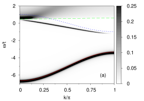
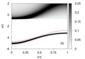
Figure 3: (Color online) Contour plot of the DOS $\rho_{\downarrow}(k,\omega)$ for (a) model I and (b) model II. The full red lines are the approximations given by Eq. (25) and (26) and the dashed green lines show the predicted onset of the continuum at $\text{min}_{q}(E_{k-q,\uparrow}+\Omega_{q})$. The dotted blue line in panel (a) shows the approximation of Eq. (27). Parameters are $J_{0}=5t$, $J=0.05t$, $S=\frac{1}{2}$ and $\eta=0.01t$ in (a), $\eta=0.02t$ in (b).

The nature of the spin-polaron can be understood by considering the limit $J_{0}\gg t,J$. We start with model II. The interaction $\mathcal{H}_{ex}^{(II)}$ is minimized by an on-site singlet between the carrier and its spin:

$$|s\rangle_{i}=\frac{1}{\sqrt{2S+1}}\left\{\sqrt{2S}c_{i,\downarrow}^{\dagger}-\frac{1}{\sqrt{2S}}c_{i,\uparrow}^{\dagger}S_{i}^{-}\right\}|{\rm FM}\rangle,$$ (24)

with eigenenergy $-\frac{J_{0}}{2}(S+1)$. Strictly speaking, this is a singlet only for $S={1\over 2}$, but we will use this term in the following. Hopping $\hat{T}$ lifts the degeneracy, and to first order in $t$ and $J$ the spin-polaron energy is given by:

$$E_{P}^{(II)}(k)=-\frac{J_{0}}{2}(S+1)+\frac{2S}{2S+1}\epsilon(k)+\frac{2JS}{2S+1}.$$ (25)

The spin-polaron state $|P_{II},k\rangle=\frac{1}{\sqrt{N}}\sum_{i}e^{ikR_{i}}$ $|s\rangle_{i}$ thus describes a singlet, or bound state between the carrier and a magnon at the same site, which propagates with an effective hopping amplitude $2St/(2S+1)<t$, suppressed because of magnon cloud overlap. The last term is the FM exchange energy lost in the magnon’s presence. The full (red) line in Fig. 3(b) shows this variational approximation, which is already quite accurate even for $J_{0}=5t$. In fact, Eq. (25) gives a reasonable approximation for the $k\approx 0$ part of the polaron dispersion down to $J_{0}\sim t$, showing that this picture of the polaron as a local singlet between the carrier and its spin is quite robust. What happens as $J_{0}$ decreases is that the polaron band moves closer to the continuum, and the $k\rightarrow\pi$ part of its dispersion “flattens out” below the continuum, in typical polaronic fashion (for more details, see Ref. FM, ).

Similar considerations apply to model I. Here, $\mathcal{H}_{ex}^{(I)}$ is minimized by the three-spin polaron (3SP):3SP

$$|3SP\rangle_{i+\frac{1}{2}}=\sqrt{4S\over 4S+1}\left\{c_{i+\frac{1}{2},\downarrow}^{\dagger}-c_{i+\frac{1}{2},\uparrow}^{\dagger}\frac{S_{i}^{-}+S_{i+1}^{-}}{4S}\right\}|{\rm FM}\rangle$$

with eigenenergy $-J_{0}(S+\frac{1}{2})$. It describes a bound state between the carrier and a magnon on either of the neighbor spin sites. Hopping lifts the degeneracy and, to first order in $t$ and $J$, the energy of the polaron eigenstate $|P_{I},k\rangle=\frac{1}{\sqrt{N}}\sum_{i}e^{ikR_{i+\frac{1}{2}}}|3SP\rangle_{i+\frac{1}{2}}$ is:

$$E_{P}^{(I)}(k)=-J_{0}\left(S+\frac{1}{2}\right)+\epsilon(k)\frac{4S+{1\over 2}}{4S+1}+\frac{JS}{4S+1}.$$ (26)

This expression is shown as a full (red) line in Fig. 3(a), and is in very good agreement with the exact dispersion already for $J_{0}=5t$. The agreement remains reasonable down to $J_{0}=t$ at $k\approx 0$, indicating that the description of this spin-polaron as a propagating 3SP is also robust.

For sufficiently large $J_{0}$ values, model I has a second discrete state below the continuum. This is based on an excited state of $\mathcal{H}_{ex}^{(I)}$. In the $J_{0}\gg t,J$ limit, it leads to $|P_{I}^{*},k\rangle=\frac{1}{\sqrt{4SN}}\sum_{i}e^{ikR_{i+\frac{1}{2}}}c_{i+\frac{1}{2},\uparrow}^{\dagger}(S_{i}^{-}-S_{i+1}^{-})|{\rm FM}\rangle$, with energy:

$$E_{P^{*}}^{(I)}(k)=\frac{J_{0}}{2}(2S-1)-\frac{1}{2}\epsilon(k)+JS.$$ (27)

The agreement between this approximation (thin blue line) and the exact result shown in Fig. 3(a) is rather poor, especially close to the continuum, but it improves with increasing $J_{0}$. More details on these additional states are discussed in Ref. FM, , in a 2D context.

To summarize the results so far, in the $S_{\text{tot}}^{z}=NS-{1\over 2}$, one-carrier sector, all three models have a low-energy, infinitely lived quasiparticle. The mapping from model II to model III is straightforward, since the polaron of model II has a singlet-like core, precisely like the “hole” of model III. Of course, a proper mapping requires some rescaling of the parameters: the “hole” hopping integral is different from that of the charge carrier itself. The discussion above identified the origin of this rescaling (polaron cloud overlap) and the expected renormalization.

At first sight, the polarons of model I and II seem to be quite different. However, we can rewrite

$$|P_{I},k\rangle=\sum_{i}\frac{e^{ikR_{i}}}{\sqrt{2N}}\left(\sqrt{2S}d_{k,i,\downarrow}^{\dagger}-\frac{1}{\sqrt{2S}}d_{k,i,\uparrow}^{\dagger}S_{i}^{-}\right)|{\rm FM}\rangle,$$

i.e. as a singlet between the carrier in an “on-site” orbital $d_{k,i,\sigma}^{\dagger}=\frac{1}{\sqrt{4S+1}}\left(e^{i\frac{k}{2}}c_{i+\frac{1}{2},\sigma}^{\dagger}+e^{-i\frac{k}{2}}c_{i-\frac{1}{2},\sigma}^{\dagger}\right)$, and its local spin. This is exactly like the polaron of model II if we replace $d_{k,i,\sigma}\rightarrow c_{i,\sigma}$.

These $d_{k,i,\sigma}$ operators are similar to the $P_{i,\sigma}^{(S)}$ operators in the Zhang-Rice approach: they are linear combinations of carrier orbitals at sites neighboring a spin-site, and they are not orthogonal to one another. The main difference is that our linear combinations have $k$-dependent phases. This allows us to avoid the need for a diverging normalization factor $\beta_{\bf k}$ in $|P_{I},k\rangle$, which then lead to the introduction of the much more complicated orbitals $\phi_{i\sigma}$ in the ZRS.ZR While the discussion here is for 1D, similar considerations hold in 2D.FM

What we found so far, then, is that all three models have the same low-energy physics in the non-trivial single-carrier sector: the low-energy state is an infinitely lived quasiparticle in all cases, with a polaron core similar to a ZRS. This suggests that we can indeed model the low-energy physics of the two-sublattice, two-band Hamiltonian with a much simpler $t$-$J$ model for “holes”, similar to Zhang and Rice’s mapping of the two-sublattice, three-band Emery model to a $t$-$J$ model for ZRS. The next question is whether this mapping also describes well the interactions between quasiparticles.

V.2 Two charge carriers in the $S^{z}_{\rm tot}=NS$ sector

As already mentioned, if both carriers have spin up ($S^{z}_{\rm tot}=NS+1$), there are no interactions between them. If both are injected with spin down ($S^{z}_{\rm tot}=NS-1$), the magnon-mediated interactions turn out to be weak or repulsive and there is no qualitative difference between the low-energy spectra of these models, as we discuss at the end of this section.

The interesting case is the $S^{z}_{\rm tot}=NS$ sector, i.e. when one carrier is injected with spin up and the other one with spin down. As we show now, here we can identify qualitative differences between models I and II (model III cannot be used here, since it does not distinguish between a spin-up carrier and a lattice spin).

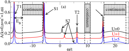
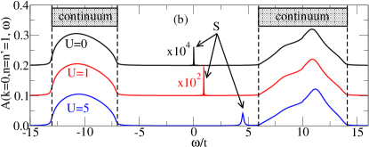
Figure 4: (Color online) Spectral function $A(k=0,n=n^{\prime}=1,\omega)$ for model I (a) and model II (b). Dashed lines mark the expected continuum boundaries. Discrete states, i.e. bipolarons, are labeled according to their symmetry, S for singlet-like and T for triplet-like. Parameters are $J_{0}=20t$, $J=0.05t$, $S=1/2$, $\eta=0.1t$ and $U/t=0,1,5$.

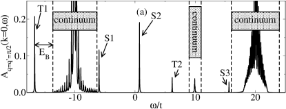
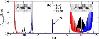
Figure 5: (Color online) (a) $A_{q=q^{\prime}=\frac{\pi}{2}}(k=0,\omega)$ for model I. Using $q=q^{\prime}=\frac{\pi}{2}$ ensures that states with both symmetries have non-vanishing weight. (b) $A_{q=q^{\prime}=0}(k,\omega)$ for model II and $k=0,\pi,2\pi$. Dashed lines mark the expected continuum boundaries. Discrete states, i.e. bipolarons, are labeled according to their symmetry, S for singlet-like and T for triplet-like. Parameters are $J_{0}/t=20$, $J/t=0.05$, $S=1/2$, $U/t=0$, $\eta/t=0.02$ and $N=60$ for (a), $N=50$ for (b).

$A(k=0,n=n^{\prime}=1,\omega)=-\frac{1}{\pi}\text{Im}G(n=n^{\prime}=1,k=0,\omega)$ obtained with the real-space solution for both models are shown in Fig. 4. Their counterparts $A_{q,q^{\prime}}(k=0,\omega)=-\frac{1}{\pi}\text{Im}G(k=0,q,q^{\prime},\omega)$, are shown in Fig. 5. Since both methods are exact, these spectral weights must have poles at exactly the same eigenenergies, however the weight at these poles differs since we are projecting on different types of states. In both cases spectra are displayed for $J_{0}/t=20$, $J/t=0.05$ and $S=\frac{1}{2}$. The value of $J_{0}$ was chosen so large intentionally in order to spread out the different features of the spectrum.

In the absence of interactions, the spectrum for two carriers equals the convolution of the corresponding one-particle spectra, which are known. This is why we expect to see a high energy continuum describing scattering states consisting of two spin-up carriers and a magnon, spanning energies $\{E_{q,\uparrow}+E_{q^{\prime},\uparrow}+\Omega_{k-q-q^{\prime}}\}_{q,q^{\prime}}$, arising from the convolution between the high-energy continuum in the spin-down carrier spectrum and the spin-up carrier eigenstate. Neglecting a small $J$ term, the edges of this continuum are at $\pm 4t+2\gamma J_{0}S$, i.e. $[16t,24t]$ for model I and $[6t,14t]$ for model II, for these parameters. These values are marked by the dashed vertical lines.

The real-space solution indeed shows a high-energy continuum for both models at precisely the expected locations. However, the k-space solution (Fig. 5(a)) has finite weight only in part of the continuum. The reason for this is that here we project on delocalized states where each carrier has a well defined momentum $\frac{k}{2}\pm q$. Depending on $k$ and $q$, sections of the continuum have vanishing overlap with these states. This is confirmed in Fig. 5(b), where $A_{q=q^{\prime}=0}(k,\omega)$ is shown for $k=0,\pi,2\pi$. Taken together, the three curves cover the full interval where the continuum is expected. Note that the spectrum for $k=2\pi$ is different from that for $k=0$, since for the former we project on states $c_{\pi,\uparrow}^{\dagger}c_{\pi,\downarrow}^{\dagger}|{\rm FM}\rangle$, whereas for the latter we project on $c_{0,\uparrow}^{\dagger}c_{0,\downarrow}^{\dagger}|{\rm FM}\rangle$.

The k-space solution also has oscillating weight inside the continua. This is a finite-size effect due to the relatively small value of $N=60$ unit cells, and can be fixed using a larger $N$. However, since here we project on delocalized states, an increase in $N$ results in a smaller weight for all bound states, as already discussed. Therefore, for our purposes it is not beneficial to use a larger $N$.

Next, the convolution of the polaron state and the spin-up state must result in a low-energy continuum $\{E_{P}^{(I,II)}(q)+E_{k-q,\uparrow}\}_{q}$. Using the asymptotic expressions from Eqs. (25) and (26) for the polaron energies and ignoring the small $J$ term, for $k=0$ the edges of this continuum are at $\pm 2t\left(1+\frac{4S+{1\over 2}}{4S+1}\right)-\frac{J_{0}}{2}$ for model I and at $\pm 2t\left(1+\frac{2S}{2S+1}\right)-\frac{J_{0}}{2}$ for model II, respectively. For the parameters of Figs. 4 and 5 this corresponds to $[-13.7t,-6.3t]$ and $[-13t,-7t]$, respectively. These values are marked by vertical dashed lines and are also in excellent agreement with the low-energy continua found by the exact solutions (similar considerations to those discussed above apply to the k-space solution).

For large values of $J_{0}/t$ the spin-down carrier spectrum of model I has the additional discrete state between the polaron band and the continuum (cf. Fig. 3). This should also give rise to a continuum $\{E_{P^{*}}^{(I)}(q)+E_{k-q,\uparrow}\}_{q}$, which corresponds to $[9t,11t]$ for these parameters. This continuum is absent in the real-space solution. This is not surprising because the asymptotic expression for $|P_{I}^{*},k\rangle$ has zero overlap with any state with a spin-up and a spin-down carrier like those used in the projection. In reality, there are small corrections to this asymptotic expression and indeed, the k-space solution shows a (restricted) continuum here, with a weight that is indeed orders of magnitude smaller than for the other two continua.

We conclude that there is excellent agreement between the continua displayed by the exact solutions, and those expected based on the convolutions of the corresponding one-carrier spectra; this is a good consistency check.

If there are sufficiently strong interactions between carriers so as to bind them in pairs, this should result in discrete states appearing in the spectrum outside these continua. The exact solutions show five such states for model I, and one for model II.

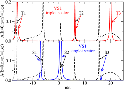
Figure 6: (Color online) Exact spectral weight $A(k=0,n=n^{\prime}=1,\omega)$ (dashed black line) and the corresponding VS1 predictions in the triplet-like (top panel, full red line) and singlet-like (bottom panel, full blue line), for model I. Parameters are $J_{0}/t=20,J/t=0.05,U/t=0,S=1/2,\eta/t=0.1$.

We have checked that these are indeed discrete states (as opposed to very narrow continua) by verifying that they are Lorentzians of width $\eta$.Mirko This finite width is responsible for the apparent overlaps of S1 and S3 with their nearby continua, but they become distinct features as $\eta\rightarrow 0$. The nature of these states is further confirmed in Fig. 6, where we compare the exact spectral weights to the predictions of VS1 for the triplet-like (top panel) and singlet-like (bottom panel) sectors. Eqs. (21)-(23) predict three peaks in the triplet-like sector. The lower two are in good agreement with two of the exact peaks; the third falls in the center of a continuum, and is therefore not indicative of a true bound-state. In the singlet-like sector, VS1 predicts three peaks as well. The lowest and highest of these happen to fall at the edge of continua. A more accurate approximation like VS2 shows that they are pushed just outside those continua, where indeed there are discrete states in the exact solution. The central peak also agrees well with a discrete peak in the exact solution. For model II, VS1 finds one singlet peak, in agreement with the peak appearing near $\omega\sim U$ in the exact solution.Mirko

Since the variational solutions include only states where the carriers are confined to be close to one another, the good agreement with the discrete states of the exact solutions validates the latters’ identification as bound states, i.e. bipolarons. Their triplet-like or singlet-like symmetry at $k=0$ is also in perfect agreement with what is inferred from the exact solution by looking at the relative phases of the $n=1$ and $n=-1$ Green’s functions, for example. As mentioned, at $k\neq 0$ these states no longer have a definite symmetry.

From the VS or from the dependence on $n$ of $G(n,n^{\prime},k,\omega)$ at energies $\omega$ close to one of these peaks, we can infer the underlying nature of these polarons. For example, the bound state of model II has most of its weight on the configuration where both carriers are on the same site, i.e. $|k=0,n=0\rangle$. This explains the small spectral weight for this state in Fig. 4(b), where we project on $|k=0,n=1\rangle$ states whose contribution is exponentially smaller, especially for smaller $U$. It also explains the strong dependence of its energy on $U$: having both carriers on the same site costs $U$. Finally, it also explains why the energy of this state hardly depends on $J_{0}$: the carriers form a singlet with each other when on the same site, and there is no exchange between this singlet and the lattice spins. As a result, this state of energy $\omega\sim U$ is always located above the low-energy spin-up carrier+polaron continuum, whose energy is $\sim-J_{0}/2$ lower because of exchange between carriers and spins. This state (which is very similar to S2 of model I) has a non-monotonic dispersion with $k$ in certain regions of the parameter space.Mirko However, it is rather uninteresting overall, since it is not bound by magnon-mediated interactions and, moreover, it is a high-energy state.

In contrast, model I has a triplet-like bipolaron (T1) as its low-energy eigenstate, in addition to four other higher energy bipolaron states. While we can analyze and understand the nature of all these higher-energy bipolarons, in the following we focus on the low-energy bound state which is of primary interest to us.

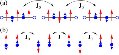
Figure 7: (Color online) (a) The three highest-weight configurations of the low-energy T1 bipolaron of model I, illustrating the magnon-mediated interaction that binds the carriers. There are matrix elements of order $J_{0}$ between these states, due to carrier-spin spin-flip processes. (b) A possible analogue in model II for the magnon-exchange process shown in (a). The central matrix element is now of order $J$. Symbols have the same meaning as in Fig. 2.

V.3 The low-energy bipolaron of model I

The three configurations with the highest-weight contributions to this bipolaron’s wavefunction are depicted in Fig. 7(a). They clearly illustrate the underlying mechanism responsible for binding the two carriers as being due to the back-and-forth exchange of a magnon, which is emitted by the spin-down carrier and then absorbed by the other, initially spin-up carrier. This process is facilitated by the fact that the carriers sit on adjacent sites and simultaneously interact with the lattice spin located between them. The triplet-like symmetry at $k=0$ is a consequence of the fact that the symmetric combination (bonding state) has the lowest energy, all the more so since it also avoids the cost of the on-site repulsion $U$. Indeed, Fig. 4(a) confirms that the energy of this state is independent of $U$.

In Fig. 7(b) we sketch what would be the analog in model II for this magnon-mediated interaction. Because here each carrier interacts only with its own spin, the magnon has to hop from one site to the other. This is a process controlled by $J$, which is the smallest energy scale. As such, it is not sufficient to bind the two carriers together, and indeed we find no such bound states in the low-energy spectrum of model II. Clearly, having carriers and spins on different sublattices greatly facilitates the magnon-mediated interactions in model I.

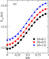
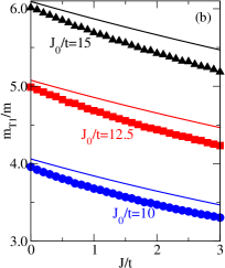
Figure 8: (Color online) (a) The dispersion of the low-energy T1 bipolaron of model I, for $J_{0}/t=15$ and $J/t=0.1,0.5,1$. (b) Bipolaron mass in units of the free carrier mass, $m_{T1}/m$, as a function of $J/t$ for $J_{0}/t=10,12.5,15$. Other parameters are $S=\frac{1}{2}$, $\eta/t=0.02$. Symbols are the exact results obtained with the real-space solution, while solid lines give a perturbative approximation discussed in the text.

The dispersion $E_{\text{T1}}(k)$ of this low-energy bipolaron is plotted in Fig. 8(a) for three values of $J$. Changing $J$ shifts the curves vertically, as expected since the FM exchange energy lost in the presence of the magnon is increased. However, the shape of these curves does not change much, confirming the fact that the binding and dynamics of the bipolaron are primarily controlled by $J_{0}$ and $t$. The dispersion is consistent with nearest-neighbor hopping, but with a renormalized effective mass.

The bipolaron mass expressed in terms of the free carrier mass is shown in Fig. 8(b) vs. $J/t$, for several values of $J_{0}/t$. These bipolarons are remarkably light, with $m_{T1}/m\approx 4$ for $J_{0}/t=10$ and further decreasing with decreasing $J_{0}$ and/or increasing $J$.

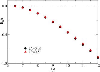
Figure 9: Bipolaron binding energy $E_{B}$ as a function of $J_{0}$ for two values of $J$. These exact values are for $S={1\over 2}$, and are independent of $U$. The bipolaron unbinds if $J_{0}/t<6.5t$.

To understand these trends, we used Rayleigh-Schrödinger perturbation theory to third order in $t$ and $J$.Sakurai Details are summarized in Appendix D. The results are shown by the full lines in Fig. 8, and are in reasonable agreement with the exact results. In particular, for $S={1\over 2}$ we find the bipolaron effective mass to be:

$$\frac{m_{\text{T1}}}{m}= \frac{0.406J_{0}^{2}/t}{J_{0}+0.570J}\approx 0.406\frac{J_{0}}{t}-0.231\frac{J}{t}.$$ (28)

The dependence on $J_{0}$ and $J$, which agrees with that displayed by the exact results, can be understood as follows. Consider moving the 3 configurations shown in Fig. 7(a) by one site to the right. For the left and the right configurations, this can be done simply with two consecutive hops of the two charge carriers. However, for the central configuration, hopping the first carrier to the right costs an energy of order $J_{0}$, since it leaves the vicinity of the magnon. Hopping the second carrier then leaves the magnon “behind”. This can be fixed either by absorbing the magnon first and thus switching to one of the other two configurations, or, for large enough $J$, the magnon has a high probability to hop on its own. Of course, in reality things are more complicated, but this analysis gives a rough idea why an increase in $J$ and/or decrease in $J_{0}$ makes the bipolaron more mobile.

So far, results have been shown for values of $J_{0}/t$ that are rather unphysically large. The final question to address is what happens for smaller values of $J_{0}/t$. The answer is provided in Fig. 9, where we plot the evolution of the bipolaron binding energy $E_{B}$ (measured with respect to the lower edge of the low-energy continuum, see Figs. 4(a) and 5(a)) with $J_{0}/t$. For negative values of $E_{B}$ the bipolaron is below the continuum and therefore stable, while $E_{B}\rightarrow 0$ means that the magnon-mediated interaction is no longer sufficient to bind the bipolaron and instead it dissociates into the continuum of states with a polaron plus a spin-up carrier.

Fig. 9 shows that the bipolaron is stable only for $J_{0}/t\gtrsim 6.5$, roughly independent of the value of $J$ and certainly independent of the value of $U$. This is consistent with the fact that $J_{0}$ controls the magnon-mediated interaction in model I, and that this interaction must be sufficiently large to compensate for the loss of kinetic energy in order to bind the carriers.

An in-depth analysis of the significance of these results is offered in the last section. Here we conclude by noting the extreme importance of the lattice structure to the low-energy physics in the two-carrier sector. Because in model I the two carriers can simultaneously interact with the same spin, the magnon-mediated exchange is very efficient and results in a strong effective attraction that can stabilize a bipolaron. In model II, a spin can interact at most with one carrier at a time. As a result, the magnon-mediated interaction is very weak and low-energy bipolarons do not form. The two models are no longer qualitatively similar in this two-carrier sector.

V.4 Two spin-down carriers

It is possible to obtain the exact $T=0$ solution in the two-carrier, $S^{z}_{\rm tot}=NS-1$ subspace with the real-space formalism. The only complication is that spin-flip processes link the two spin-down carrier states both to states with one magnon and one spin-up carrier, and to states with two magnons and both carriers with spin-up. Thus, we can now have up to four particles (carriers or magnons) in the system, but this can be handled by the formalism introduced in Ref. FewP, .

However, perturbational arguments described next show that it is always energetically unfavorable for a low-energy bipolaron to form in this sector. The lowest energy feature is, therefore, the two-polaron continuum whose location is already known to be $\{E_{P}^{(I,II)}(k-q)+E_{P}^{(I,II)}(q)\}_{q}$, and the full calculation becomes unnecessary. In model III, the situation is qualitatively similar since no interactions appear between two “holes”.

Consider model I in the limit $t\rightarrow 0,J\rightarrow 0$. If the two carriers are two or more sites apart then each forms a 3SP, and the total energy is $2E_{\text{P}}^{(I)}\rightarrow-J_{0}(2S+1)$. If the carriers are on neighboring sites, simultaneous interactions with the central spin change this energy to a value that is calculated easily by exact diagonalization. We findMirko that this energy is larger than $2E_{\text{P}}^{(I)}$ for any $S$ and $J_{0}$, in other words it is energetically favorable to keep the 3SP spatially apart. Thus, in model I the magnon-mediated interactions are repulsive in this spin-sector. In model II, these interactions are very weak because each charge carrier interacts only with its own spin/magnon. Turning on the hopping will further favor unbound polarons, since they are lighter and therefore can lower their kinetic energy more than a bipolaron.

This is why we do not expect low-energy bound states in any of these models, in this sector, so we do not consider it any further.

VI Summary and discussion

In this article we used exact, $T=0$ solutions for one and two carriers doped in a ferromagnetic background to compare the low-energy physics of three different models. The goal was to understand if the simpler models describe the same low-energy physics as the more complex one.

In the single-carrier sector this turned out to be the case: all three models have a low-energy polaron whose core can be thought of as a singlet between the carrier and a local spin. In the two-sublattice model I, a 3SP description is more appropriate but it can be reduced to a propagating singlet using a construction somewhat similar to the ZRS. Based on this, one could conclude that a simple one-band model provides an appropriate description for carriers in a FM background.

However, results from the two-carrier sector paint a different picture, especially when the carriers are injected with opposite spins. Here, for the two-sublattice model we find that the ability of both carriers to interact simultaneously with a common spin leads to an attractive, magnon-mediated interaction, of order $J_{0}$. Such an interaction is evidently not included in a $t$-$J$ model, where the $J_{0}$ energy scale was integrated out. In fact, for the FM background we cannot even use the $t$-$J$ model to describe this case, because “holes” only appear when doping with spin-down carriers, and there is no counterpart for a spin-up carrier. This is why here we studied the intermediate model II, where we know that a spin-down carrier can form its singlet-like “hole”, but we can also treat spin-up carriers. The fact that in model II only one carrier can interact with a given spin, however, leads to a very different mechanism for the magnon-mediated interaction. In particular, the strong attraction that appears in model I does not arise in model II.

Similar differences appear in the two spin-down sector. We argued that here each carrier forms its polaron and they move independently, so the “big picture” seems to be the same in all the models: none gives rise to a strong-enough magnon-mediated attraction to be able to bind the polarons. However, there are differences in details. As discussed in the last subsection, for model I here we expect a local repulsion between polarons, again controlled by $J_{0}$, due to the additional exchange cost when the two spin-down carriers are forced on neighboring sites and frustrate each other in forming their 3SP clouds. In contrast, in model II each spin-down carrier can form a singlet with its spin, and there is no difference if they are neighbors or not; hence, there is no counterpart to the magnon-mediated repulsion of model I. Model III, on the other hand, has only very weak interactions between its “holes”, due to the fact that if they are on neighbor sites they break fewer FM bonds then if they are farther apart. This very weak attraction is of order $J$ and describes completely different physics.

Since the magnon-mediated interactions that arise between carriers are very different in the three models, it is clear that they do not describe the same low-energy physics in cases with two or more carriers, even though their quasiparticles are similar in nature. We therefore conclude that the two-sublattice model cannot be replaced by simple one-lattice models, whether with one or with more bands, because these no longer allow two carriers to interact simultaneously with the same lattice spin and, as a result, completely change the nature of the magnon-mediated interactions.

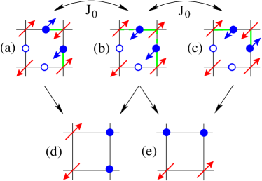
Figure 10: (Color online) (a), (b) and (c) depict two-hole configurations on a CuO₂ layer, connected to one another by spin-flip processes of order $J_{0}$. These are the 2D analogs of Fig. 7(a), and describe the main mechanism for magnon-mediated attraction between holes. (d) and (e) show their corresponding one-band configurations, obtained by locking the holes in ZRS with a neighbor Cu spin. The thick light green lines in (a), (b) and (c) show which hole can pair with which spin. For (b), there are two possible pairing options, indicated by full and dashed thick green lines, respectively.

While each new problem has to be considered carefully, we expect that this situation may be the rule rather than an exception. The reason is that the ZRS-like states on which the simpler models are built mix together charge and spin degrees of freedom. As such, it seems unlikely to us that the magnon-mediated interactions between carriers could be easily “mimicked” by simple effective interactions between these complex objects.

Even though all our exact results are for a FM background, we think that simple arguments show that these claims extend to AFM backgrounds. Consider, for instance the situation sketched in Fig. 10(a), with two neighboring holes on a CuO₂-like lattice. For simplicity, we assume that the Cu spins are well-described by Néel order on the length scale of interest here.

In the two-sublattice model, configuration (a) is connected through matrix elements of order $J_{0}$ to configurations (b) and (c). This is the 2D analog of the exchange of a magnon through the common lattice spin depicted in Fig. 7(a), i.e. precisely the process expected to be responsible for the magnon-mediated interactions between carriers. If we lock these holes into ZRS and map configuration (a) to a one-band model, we obtain the state of Fig. 10(d). Configuration (b) can map to the same one-band state (d), because it is part of the same ZRS as (a), but it can also map to configuration (e), depending on how we choose which hole pairs with which spins. Finally, configuration (c) maps to (e), as expected since it is part of the same ZRS as (b).

The problem is now obvious: the one-band $t$-$J$ model has no matrix element between states (d) and (e), never mind one of order $J_{0}$ (this energy scale has been removed from this model). As such, it clearly fails to describe the same physics as the two-sublattice model, since it grossly underestimates the strength of the magnon-mediated attraction between carriers. Instead of this back-and-forth exchange of the magnon that strongly favors configurations with neighbor carriers, the $t$-$J$ model only describes weak interactions of order $J$ between “holes” because of the number of AFM bonds broken as they move around and reshuffle the lattice spins; this is completely different physics. This example explains why we believe that simple one-band models cannot be expected to describe properly interactions between carriers.

Two possible ways to fix the problem can be envisioned. One is to add additional terms in the one-band Hamiltonians to generate the missing matrix elements. For example, states (d) and (e) in Fig. 10 could be connected by a term describing second-nearest neighbor hopping of a hole if there is a second hole in its vicinity. Similar “conditional” third nearest-neighbor hopping must also be included for configurations where the holes are on the same line. These terms would strongly favor pairing of the carriers, especially since they do not disturb the AFM background order. In fact, since $J_{0}$ is a large energy scale, this might explain the existence of rather mobile pre-formed pairs, which is one of the favorite scenarios to explain the pseudo-gap regime.

While this way to fix the one-band models is appealing, care is needed to make sure that all these additional matrix elements have the proper signs (i.e., like those arising in the more complex model); and also that the effects of other processes, such as the spin-swap termsBayo1 which we have not included in this model, are properly accounted for and “mimicked”. It should also be explored what, if any, are the consequences of the fact that multiple states in the one-band Hilbert space may correspond to a single state of the two-sublattice model, as shown in Fig. 10 for configurations (b), (d) and (e) (note that there is also a third one-band configuration corresponding to (b), with the ZRS diagonally opposite to each other).

The alternative is to study the proper two-sublattice models. They have larger Hilbert spaces, unfortunately, but at least they are certain to describe correctly the significant magnon-mediated attraction between carriers, which may well be responsible for most, if not all, the glue needed for superconductivity in cuprates.

Appendix A Details for the real-space solution for the two-carrier case

The EOM for model I are:

$$G(n,n^{\prime},k,\omega)= \frac{1}{\omega+i\eta}\left\{\vphantom{\sqrt{\frac{S}{2}}}\delta_{n,n^{\prime}}-2t\cos\frac{k}{2}\left[G(n+1,n^{\prime},k,\omega)+G(n-1,n^{\prime},k,\omega)\right]\right.$$ .

$$\left.+J_{0}\sqrt{\frac{S}{2}}\left[G(n,n,n^{\prime},k,\omega)+G(n,n+1,n^{\prime},k,\omega)\right]\right\}, \text{for}\ n>0,$$ (29)

$$G(n,n^{\prime},k,\omega)= \frac{1}{\omega+i\eta}\left\{\vphantom{\sqrt{\frac{S}{2}}}\delta_{n,n^{\prime}}-2t\cos\frac{k}{2}\left[G(n+1,n^{\prime},k,\omega)+G(n-1,n^{\prime},k,\omega)\right]\right.$$ .

$$\left.-J_{0}\sqrt{\frac{S}{2}}\left[G(-n,0,n^{\prime},k,\omega)+G(-n,1,n^{\prime},k,\omega)\right]\right\}, \text{for}\ n<0,$$ (30)

$$G(0,n^{\prime},k,\omega)= \frac{1}{\omega-U+i\eta}\left\{\vphantom{\sqrt{\frac{S}{2}}}\delta_{0,n^{\prime}}-2t\cos\frac{k}{2}\left[G(1,n^{\prime},k,\omega)+G(-1,n^{\prime},k,\omega)\right]\right\},$$ (31)

$$G(n,m,n^{\prime},k,\omega)= \frac{1}{\omega-2JS-\frac{J_{0}}{2}[4S-\delta_{m,0}-\delta_{m,1}-\delta_{m,n}-\delta_{m,n+1}]+i\eta}$$

$$\times\left\{-t\left[e^{-i\frac{k}{2}}(1-\delta_{n,1})G(n-1,m-1,n^{\prime},k,\omega)+e^{i\frac{k}{2}}G(n+1,m+1,n^{\prime},k,\omega)\right.\right.$$

$$\left.\left.\vphantom{e^{i\frac{k}{2}}}+e^{-i\frac{k}{2}}G(n+1,m,n^{\prime},k,\omega)+e^{i\frac{k}{2}}(1-\delta_{n,1})G(n-1,m,n^{\prime},k,\omega)\right]-JS\left[G(n,m+1,n^{\prime},k,\omega)\right.\right.$$

$$\left.\vphantom{e^{i\frac{k}{2}}}\left.+G(n,m-1,n^{\prime},k,\omega)\right]+J_{0}\sqrt{\frac{S}{2}}[(\delta_{m,n}+\delta_{m,n+1})G(n,n^{\prime},k,\omega)\right.$$

$$\left.\vphantom{e^{\frac{k}{2}}}-(\delta_{m,0}+\delta_{m,1})G(-n,n^{\prime},k,\omega)]\right\},\ \text{for}\ n\geq 1,\ -\infty<m<\infty.$$ (32)

Appendix B Solution for $G(0,0,k,\omega)$

We show here how to calculate $G(0,0,k,\omega)$. From Eq. (31) we see that $G(0,0,k,\omega)$ is linked only to $G(\pm 1,0,k,\omega)$. We can choose to order the vectors $\mathbf{V}_{M}$ in such a way that $G(1,0,k,\omega)=[\mathbf{A}_{1}]_{1,1}G(0,0,k,\omega)$ and $G(-1,0,k,\omega)=[\mathbf{A}_{1}]_{2,1}G(0,0,k,\omega)$. Inserting this into Eq. (31) we find:

$$G(0,0,k,\omega)=\frac{1}{\omega+i\eta-U+2t\cos\frac{k}{2}([\mathbf{A}_{1}]_{1,1}+[\mathbf{A}_{1}]_{2,1})},$$

where $\mathbf{A}_{1}$ is obtained from the recursive relation Eq. (18). Once $G(0,0,k,\omega)$ and therefore $\mathbf{V}_{0}$ is known, one can use the recursive relation Eq. (17) to find $\mathbf{V}_{M}=\mathbf{A}_{M}\dots\mathbf{A}_{1}\mathbf{V}_{0}$, and thus to generate all Green’s functions corresponding to values of $M>0$.

Appendix C Details for VS1 for model I, in the triplet-like sector

We introduce the shorthand notation:

$$a^{+}_{1}=_{+}\!\!\langle k,1|\hat{G}(\omega)|k,1\rangle_{+},$$ (33)

$$a^{+}_{1,1}=_{+}\!\!\langle k,1|\hat{G}(\omega)|k,1,1\rangle_{+},$$ (34)

$$a^{+}_{1,m}=_{+}\!\!\langle k,1|\hat{G}(\omega)|k,1,m\rangle_{+}\ \text{ for}\ m<1,$$ (35)

and using Eqs (29)-(32) we obtain the following EOM:

$$a^{+}_{1}=\frac{1+J_{0}\sqrt{\frac{S}{2}}(a^{+}_{1,0}+\sqrt{2}a^{+}_{1,1})}{\omega+i\eta},$$ (36)

$$a^{+}_{1,1}=\frac{J_{0}\sqrt{\frac{S}{2}}\sqrt{2}a^{+}_{1}-JS\sqrt{2}a^{+}_{1,0}}{\omega+i\eta-2JS-J_{0}(2S-1)},$$ (37)

$$a^{+}_{1,0}=\frac{J_{0}\sqrt{\frac{S}{2}}a^{+}_{1}-JS\sqrt{2}a^{+}_{1,1}-JSa^{+}_{1,-1}}{\omega+i\eta-2JS-J_{0}(2S-1/2)}.$$ (38)

$$a^{+}_{1,m}=\frac{-JSa^{+}_{1,m-1}-JSa^{+}_{1,m+1}}{\omega+i\eta-2JS-2J_{0}S},\ \text{for}\ m<0.$$ (39)

As appropriate for VS1, in writing the above equations we ignored all Green’s functions for basis states where the carrier-carrier distance $n\geq 2$.

The last of the above equations is a simple recurrence equation that can be solved with the ansatz $a^{+}_{1,m}(\omega)=z(\omega)a^{+}_{1,m+1}(\omega)$ (note that $m<0$). This ansatz makes use of the fact that $a_{m}^{+}(\omega)\xrightarrow{m\rightarrow-\infty}0$ and therefore requires $|z(\omega)|<1$. As previously discussed this is true because we are using a finite lifetime $1/\eta$.

Then, using $a^{\pm}_{1,-1}(\omega)=z(\omega)a^{\pm}_{1,0}(\omega)$ in Eq. (38) reduces the first 3 equations to a linear set with 3 unknowns, $a^{+}_{1},a^{+}_{1,1}$ and $a^{+}_{1,0}$. This can be solved analytically. The solution (for $J=0$, so as to keep it compact) is:

$$a^{+}_{1} =\left\{\omega+i\eta-J_{0}^{2}S\left[\frac{1}{\omega+i\eta+J_{0}(1-2S)}\right.\right.$$

$$\left.\left.+\frac{\frac{1}{2}}{\omega+i\eta+J_{0}(\frac{1}{2}-2S)}\right]\right\}^{-1}.$$ (40)

While an analytical solution is not possible in all cases, the significant reduction in the number of unknowns allows us to find very easily numerical solutions for the various VS, and therefore approximations for the energies of the bound states (if any exist).

Appendix D Effective mass of the bipolaron

The first order correction is obtained by diagonalizing $\mathcal{H}_{ex}^{(I)}$ in the subspace spanned by $|k,n=1\rangle+|k,n=-1\rangle,|k,n=1,m=1\rangle$ and $|k,n=1,m=0\rangle+|k,n=1,m=2\rangle$. Note that all of the above states have triplet-like symmetry and that this subspace is invariant under $\mathcal{H}_{ex}^{(I)}$ since this interaction cannot change the carrier-carrier distance. The lowest eigenvalue of $\mathcal{H}_{ex}^{(I)}$ in this subspace gives the zeroth order approximation for $E_{\text{T1}}$, while the first order correction in $t$ and $J$ is given by the matrix elements of $\hat{T}$ and $\mathcal{H}_{S}^{(I)}$ for the corresponding eigenvector. This results in:

$$E_{\text{T1}}^{(0)}(k)=-\frac{J_{0}}{4}\left(3-4S+\sqrt{1+16S^{2}}\right),$$

$$\Delta E_{\text{T1}}^{(1)}(k)=\frac{JS\left(2+\frac{5S\left(-1-4S+\sqrt{1+16S^{2}}\right)}{\sqrt{1+16S^{2}}}\right)}{1+3S}.$$

Note that (i) the first order correction in $t$ vanishes, since $\hat{T}$ changes the carrier-carrier distance and therefore leaves this subspace, and (ii) the zeroth order energy is identical to the VS1 result, see Eq. (21), as expected.

In order to obtain higher order corrections we need to include all the states that are linked to by $\hat{T}$ and $\mathcal{H}_{S}^{(I)}$ when starting from the configurations considered above. If need be, we also have to add whatever other configurations are necessary to ensure that the enlarged subspace is still invariant under $\mathcal{H}_{ex}^{(I)}$. This means that we need to include a total of seven additional states, some of which have singlet-like symmetry, since at finite $k$ mixing between the two symmetries occurs. However, for third order corrections one does not need to include the state where the carriers are on the same site and therefore we do not need to worry about $\hat{U}$. This may seem counterintuitive, since we are starting out with states where the carriers are on adjacent sites, i.e. $n=1$, and therefore one would expect a transition to $n=0$ to be a simple process. However, the state with $n=0$ only exists for singlet-like symmetry and since we start out with triplet-like states, the transition $n=1\rightarrow n=0$ only contributes corrections higher than third order.

For the sake of simplicity we only write here the results obtained for $S=\frac{1}{2}$:

$$\Delta E_{\text{T1}}^{(2)}(k)=-\frac{\left(275+119\sqrt{5}\right)J^{2}+40t^{2}\left(245+103\sqrt{5}+\left(205+97\sqrt{5}\right)\cos k\right)}{125\left(3+\sqrt{5}\right)^{2}J_{0}},$$ (41)

$$\Delta E_{\text{T1}}^{(3)}(k)=\frac{\left(-91+125\sqrt{5}\right)J^{3}+20Jt^{2}\left(-166+20\sqrt{5}+\left(-209+15\sqrt{5}\right)\cos k\right)}{1250J_{0}^{2}}.$$ (42)

Besides an overall shift, a dispersion proportional to $\cos(k)$ arises in the 2nd and 3rd order corrections. The effective bipolaron mass can now be extracted easily.

References

- (1) J. Zaanen, G. A. Sawatzky and J. W. Allen, Phys. Rev. Lett. 55, 418 (1985).
- (2) V. J. Emery, Phys. Rev. Lett. 58, 2794 (1987).
- (3) E. Dagotto, Rev. Mod. Phys. 66, 763 (1994); M. Ogata and H. Fukuyama, Rep. Prog. Phys. 71, 036501 (2008); P.A. Lee, Rep. Prog. Phys. 71, 012501 (2008).
- (4) F. C. Zhang and T. M. Rice, Phys. Rev. B 37, 3759 (1988).
- (5) B. Lau, M. Berciu, and G. A. Sawatzky, Phys. Rev. Lett. 106, 036401 (2011).
- (6) J. P. Carbotte, E. Schachinger and D. N. Basov, Nature 401, 354 (1999); M. Eschrig, Adv. Phys. 55, 47 (2006); T. Dahm, V. Hinkov, S. V. Borisenko, A. A. Kordyuk, V. Zabolotnyy, J. Fink, B. B chner, D. J. Scalapino, W. Hanke, and B. Keimer, Nature Phys. 5, 217 (2009); and references therein.
- (7) A. Lanzara, P. V. Bogdanov, X. J. Zhou, S. A. Kellar, D. L. Feng, E. D. Lu, T. Yoshida, H. Eisaki, A. Fujimori, K. Kishio, J.-I. Shimoyama, T. Noda, S. Uchida, Z. Hussain and Z.-X. Shen, Nature 412, 510 (2001); A. S. Alexandrov, C. Di Castro, I. Mazin, and D. Mihailovic, Adv. Condens. Matter Phys. 2010, 206012 (2010); C. Gadermaier, V. V. Kabanov, A. S. Alexandrov, L. Stojchevska, T. Mertelj, C. Manzoni, G. Cerullo, N. D. Zhigadlo, J. Karpinski, Y. Q. Cai, X. Yao, Y. Toda, M. Oda, S. Sugai, D. Mihailovic, arXiv:1205.4978, and references therein.
- (8) G. De Filippis, V. Cataudella, A. S. Mishchenko, and N. Nagaosa, Phys. Rev. Lett. 99, 146405 (2007); V. Cataudella, G. De Filippis, A. S. Mishchenko, and N. Nagaosa, Phys. Rev. Lett. 99, 226402 (2007); A. S. Mishchenko, N. Nagaosa, Z.-X. Shen, G. De Filippis, V. Cataudella, T. P. Devereaux, C. Bernhard, K. W. Kim, and J. Zaanen, Phys. Rev. Lett. 100, 166401 (2008); G. De Filippis, V. Cataudella, A. S. Mishchenko, C. A. Perroni, and N. Nagaosa, Phys. Rev. B 80, 195104 (2009).
- (9) B. Lau, M. Berciu, and G. A. Sawatzky, Phys. Rev. B 84, 165102 (2011).
- (10) T. Saitoh, A. Sekiyama, K. Kobayashi, T. Mizokawa, A. Fujimori, D. D. Sarma, Y. Takeda, and M. Takano, Phys. Rev. B 56, 8836 (1997).
- (11) G. A. Sawatzky, I. S. Elfimov, J. van den Brink, and J. Zaanen, EuroPhys. Lett. 86, 17006 (2009); M. Berciu, I. Elfimov, and G. A. Sawatzky, Phys. Rev. B 79, 214507 (2009).
- (12) M. Möller, G. A. Sawatzky and M. Berciu, Phys. Rev. Lett. 108, 216403 (2012).
- (13) J. Zaanen and A. M. Oles, Phys. Rev. B 37, 9423 (1988); D. M. Frenkel, R. J. Gooding, B. I. Shraiman and E. D. Siggia, Phys. Rev. B 41, 350 (1990).
- (14) M. Berciu and G. A. Sawatzky, Phys. Rev. B 79, 195116 (2009).
- (15) W. Nolting, Phys. Status Solidi B 96, 11 (1979); B. S. Shastry and D. C. Mattis, Phys. Rev. B 24, 5340 (1981); S. G. Ovchinnikov and L. Ye. Yakimov, Phys. Solid State 45, 1479 (2003).
- (16) M. Berciu, Phys. Rev. Lett. 107, 246403 (2011).
- (17) The reason is that consists of a hopping term for carriers (), a hopping term for magnons () and a term which creates or annihilates a magnon (), i.e. a transition between states of the type to and vice versa. The hopping terms change by if the particle that hops is located at the outside. If the hopping particle is located between the other two particles, then remains unchanged. The spin flipping term can lead to both transitions with and transitions with . The latter occur when the rightmost carrier has spin down and is flipped to create a magnon on the spin site to its right. Of course the reverse process is also possible, i.e. a magnon is annihilated and flips the spin of the carrier to its left.
- (18) Mirko Möller, Spin polarons and bipolarons on one-dimensional ferromagnetic lattices, M.Sc. Thesis, Freie Universität Berlin, 2012.
- (19) V. J. Emery and G. Reiter, Phys. Rev. B 38, 4547 (1988).
- (20) J. J. Sakurai, Modern Quantum Mechanics, (Addison-Wesley Publishing Company, 1994).