Statistical Mechanics of DNA unzipping under periodic force: Scaling behavior of hysteresis loop

Abstract

A simple model of DNA based on two interacting polymers has been used to study the unzipping of a double stranded DNA subjected to a periodic force. We propose a dynamical transition, where without changing the physiological condition, it is possible to bring DNA from the zipped/unzipped state to a new dynamic (hysteretic) state by varying the frequency of the applied force. Our studies reveal that the area of the hystersis loop grows with the same exponents as of the isotropic spin systems. These exponents are amenable to verification in the force spectroscopic experiments.

The mechanism involved in the separation of a double stranded DNA (dsDNA) into two single stranded DNA (ssDNA) is a prerequisite for understanding processes like replication and transcription. In vitro, opening of DNA is achieved either by increasing the temperature (85-90^∘C) termed as thermal melting or by changing the pH value of the solvent ($<3$ or $>9$) called DNA denaturation Wartel . However, such a drastic change in the physiological condition is not possible in living systems. The mechanism of opening of dsDNA in vivo is quite complex and is initiated by helicases, DNA and RNA polymerase, ssb proteins etc, which exert force of the order of pN and as a result DNA unwinds. It is now possible to unzip the two strands of a DNA using techniques like optical tweezers, atomic force microscopy, magnetic tweezers etc Bockelmann ; prentiss . Theoretical understanding of DNA unzipping is mostly based on equilibrium conditions bhat99 ; nelson ; Mukamel ; maren2k2 .

However, living systems are open systems and never at equilibrium. Understanding the separation of DNA in the equilibrium is one approach, but another route is to perform the analysis in a situation which closely resembles the living systems i.e. in non-equilibrium conditions. Moreover, helicases are ATP driven molecular motors. The periodic hydrolysis of ATP to ADP can generate a continuous push and pull kind of motion which spans a wide range of length and time scales. As a direct consequence of these chemo-mechanical cycles, biological machines act like a repetitive force generators, and it is believed that forces with periodic signatures are experienced by biomolecules in many physiological contexts. For instance, it has been postulated that DNA-B, a ring like hexameric helicase, pushes through the DNA like a wedge and produces unidirectional motion and strand separation dnab . Active rolling model and inchworm model are two mechanisms, which suggest that PcrA goes through cycle of pulling the ds part of the DNA and then moving on the ss part during ATP hydrolysis pcra . Williams and Jankowsy nphii showed that viral RNA helicase NPH-II hops cyclically from the ds to the ss part of DNA and back during the ATP hydrolysis cycle. Apart from these examples, there are several studies johnson ; basu ; Fili ; Szymczak , which suggest that the force acting on DNA (at the junction of the Y fork i.e. ssDNA and dsDNA) is periodic in nature rather than constant. Surprisingly, in most of the studies (experiments, theories and simulations), the applied force or loading rate is kept constant kumarphys , and hence the results provide a limited picture of the DNA opening. Application of periodic force would introduce new aspects, which are not possible in the steady force case.

In DNA unzipping, the equilibrium response of the reaction coordinate (extension ($y$)) to the constant force is well understood in terms of simple models amenable to statistical mechanics kumarphys ; marko ; kumar_prl . However, when a dsDNA is driven by an oscillatory force, $y$ will also oscillate and lag behind the force due to the relaxation delay. This relaxation delay induces hysteresis in the force-extension ($f-y$) curve, which has been recently observed in simulations and experiments mishra ; hatch ; kapri . The nature of hysteresis and its dependence on the amplitude ($F$) and frequency ($\nu$) of the applied force is well studied in the context of spin systems madan1 ; madan2 ; dd ; bkc . It is found that the area under the hysteresis loop $A_{loop}$ scales as $F^{\alpha}\nu^{\beta}$. The values of $\alpha$ and $\beta$ differ from system to system bkc . However, for DNA unzipping, the non-equilibrium response of $y$ to the oscillatory force remains elusive.

Figure 1: DNA in zipped and unzipped state. One end is fixed and the other end is subjected to a periodic force.

In this Letter, we show that under a certain physiological condition, a dsDNA remains in the steady and stable (zipped or open) state for an extended period of time. Furthermore, without any change in temperature ($T$) or pH of the solvent, by varying $\nu$ alone, a dsDNA may be brought from the time averaged open or zipped state to a new dynamic state (hysteretic), oscillating between the zipped and unzipped states, which is dynamical in origin and vanishes in the quasi static limit bkc . We evaluate the scaling exponents $\alpha$ and $\beta$ associated with $A_{loop}$, which are amenable to verification in the force spectroscopic experiments. We also show that using the work theorem ps11 , it is possible to extract the equilibrium $f-y$ curve from the non-equilibrium pathways.

We consider a simple model of DNA (Fig.1), where a string of beads (complementary nucleotides) corresponds to a single strand. The beads are connected by harmonic springs. The excluded volume and and base-pairing interactions are modeled by the Lennard Jones potential. It was recently shown that the model captures some of the essential properties of DNA and the equilibrium force-temperature diagram is in good agreement with the two state model in the entire range of the f and T mishra . In order to study the dynamical stability of DNA under the periodic force $f(t)$, we add an energy $-f(t)y(t)$ to the total energy of the system and perform Langevin Dynamics simulation to monitor the separation $y$ of the terminal base pairs sm ; arxiv . The random force $\Gamma$ sm ; arxiv , has also been super imposed on the periodic force to take account of stochastic fluctuations of the system. Here, one may fix $\nu$ and vary $F$ or keep $F$ constant and vary $\nu$. The value of $f$ increased to its maximum value $F$ in $m_{s}$ steps at interval $\Delta f(=0.01)$ and then it is taken to $0$ in the same way arxiv . Since we are interested in the non-equilibrium regime, we allow only $n$ LD time steps (much below the equilibrium time) in each increment of $\Delta f$. We keep sum of the time spent $\tau(=2nm_{s})$ in each force cycle constant to keep $\nu(=1/\tau)$ constant. In the following, we keep $T=0.1$ and $F>0.32$ text1 ; ru .

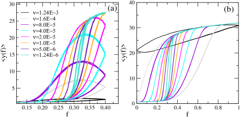
Figure 2: $\langle y\rangle$ of DNA as a function of the cyclic force of amplitudes (a) 0.4 and (b) 1.0 at different $\nu$. (a) At high $\nu$, DNA remains in the zipped state with a small hysteresis loop. As $\nu$ decreases, the system extends from the zipped state to the open state with a bigger loop. For $\nu\rightarrow 0$, the hysteresis loop vanishes and the system approaches to the equilibrium path. (b) DNA remains in the open state at high $\nu$ and approaches the equilibrium path from below as $\nu\rightarrow 0$.

In Fig.2, we plot the value of $y(f)$ (averaged over C =1000 cycles) with $f$ for different values of $\nu$. It is interesting to note that the average value of $y(f)$ for different initial conformations remains almost the same, showing that the system is in the steady state text2 . All plots show hysteresis. The area under the loop is the measure of the energy dissipated over a cycle and is defined as a dynamic order parameter bkc

$$A_{loop}=\oint y.df,$$ (1)

which depends upon $F$ and $\nu$. If $y(f)$ is less than $5$, we call the system to be in the zipped state, where as if $y(f)>5$, it is in the unzipped state arxiv . At high $\nu$, it is evident that for small $F$, dsDNA remains in the zipped state (Fig. 2a), whereas at high $F$, it is in the unzipped state (Fig. 2b), irrespective of initial conformations. Moreover, the path of $y(f)$ for the force 0 to $F$ is different from that of the path for $F$ to 0, which constitutes a hysteresis loop. A decrease in $\nu$ leads to a bigger path of the hysteresis loop sm . Depending on the amplitude, the system starts from the zipped conformation as shown in Fig. 2a (or open conformations shown in Fig. 2b) and then gradually approaches the open state (or the zipped state) and back to the initial state.

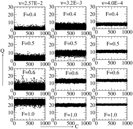
Figure 3: The time sequence of $Q$ for different $\nu$ and $F$.

One may note that even though $f$ decreases from $F$ to 0 (Fig. 2a), $y(f)$ increases and there is some lag, after which it decreases. Recall that the relaxation time is much higher compare to the time spent at each interval of $\Delta f$. Therefore, an increase in $y(f)$ with decreasing $f$ indicates that the system gets more time to relax. As a result $y(f)$ approaches a path, which is close to the equilibrium. Once the system gets enough time, the lag disappears. A similar lag is expected, when the system starts from the open state at high $\nu$. However, in this case as $\nu$ decreases, $y(f)$ decreases with increasing $f$ (Fig. 2b). In both cases , whether dsDNA starts from the zipped or open state, as $\nu\rightarrow 0$, the system approaches the equilibrium $f-y$ curve and $A_{loop}$ vanishes sm . Moreover, at high $\nu$, $A_{loop}$ also vanishes (Fig. 2a & 2b), but the system goes away from the equilibrium.

The other dynamic order parameter

$$Q=\frac{1}{\tau}\oint y(t)dt,$$ (2)

studied in the context of magnetic systems bkc , has recently been applied to obtain the the force-frequency diagram of DNA hairpin arxiv . In Fig. 3, we plot $Q$ with cycles for different $\nu$ and $F$. The distribution shows that the path remains in the zipped state or in the open state or in the dynamic (hysteretic) state, depending on $F$ and $\nu$. In contrast to the DNA hairpin, which shows the coexistence of different states, a dsDNA shows a continuous transition from the zipped state to the new dynamic state as the frequency decreases.

We now focus our study on the scaling of the area of the hysteresis loop. In Fig. 4a, we have plotted $A_{loop}$ as a function of $(F\nu)^{0.5}$. For low $\nu$, we observe that all plots for different $F$ collapse on a straight line. This gives the value of $\alpha=0.5=\beta$. At high $\nu$, depending on the amplitude, the system remains either in the zipped state (low $F$) or in the open state (high $F$). In contrast to the spin system, where the average applied field is zero over a cycle, in this case, the average applied force is finite over a cycle because the two states are asymmetric. In fact, at low $F$, we find that $A_{loop}$ scales as $\nu^{-1}(F-f_{c})^{2.0\pm 0.1}$, where $f_{c}$ is the equilibrium critical force at that temperature. The proposed scaling is consistent with the mean field values for a time dependent hysteretic response to periodic force in case of the isotropic spin dd and found to be independent of length rakesh .

In single-molecule experiments, measurements have been done at non-equilibrium conditions. It is possible to infer the equilibrium properties of the system from these data to have a better understanding of the system. In order to do so, generally measurements have been taken in the quasi static limit prentiss so that the techniques involved in thermodynamics can be employed. In recent years, there has been considerable work to extract equilibrium properties from the non-equilibrium data e.g. Jarzynski equality, which relates the free energy differences between two equilibrium states through non-equilibrium processes jarzynski . In another approach a dominant reaction pathway algorithm is developed to compute the most probable reaction pathways between two equilibrium states orland .

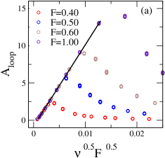
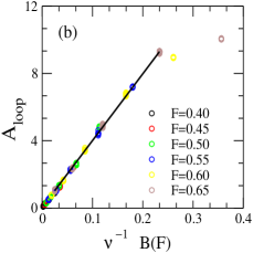
Figure 4: The scaling of the loop area of hysteresis ($A_{loop}$) with respect to $\nu^{0.5}F^{0.5}$ in the low frequency limit (a) and with respect to $\nu^{-1}B(F)$ in the high frequency limit. Here, $B(F)\sim(F-{f_{c}})^{2\pm 0.1}$ (b).

Here, we use the work theorem to derive the equilibrium path between the two states ps11 . Instead of repeating the force cycle $C$ times, we now randomly choose $C$ initial conformations, which belong to equilibrium conformations at that $T$ and $f$ (=0). We follow a similar protocol as described above to reach the final state (f=F) from the initial state (f=0). No attempt is made to achieve equilibrium during this process. The total work performed on the system going from the zipped state to open state (forward path) is $w_{m_{s}}=-{\Delta f}\sum_{i=1}^{m_{s}}y_{i}$. When the applied force decreases (backward path) from F to 0, we start with $C$ initial conformations, which belong to equilibrium conformations at that $T$ and $f$ (=F). The work done by the system from the open state to the zipped state can be written as $w_{1}={\Delta f}\sum_{i=m_{s}}^{1}y_{i}$. The equilibrium distance $y_{k}$ for the force $f_{k}$ for the forward path can be obtained by assigning the weight $exp(-\beta w_{k})$ to all forward $C$ paths ps11 at that instant $k$, which can be written as

$$y_{k}=\frac{\sum_{i}^{C}y_{k}exp(-\beta w_{k})}{\sum_{i}^{C}exp(-\beta w_{k})}.$$ (3)

Similarly, $y_{k}$ for the reverse path can also be obtained.

In Fig.5a, we have plotted the simple average of extension over many ($C=1000$) forward paths as well as backward paths ($n=10^{4}$ LD time steps). One can see the existence of hysteresis. In this figure, the solid line corresponds to the equilibrium path, which is the same, whether we start from the zipped or open conformation. We have used $2\times 10^{9}$ time steps out of which the first $5\times 10^{8}$ steps have not been taken in the averaging. The results are averaged over many trajectories, which are almost the same within the standard deviation. The weighted average of $y(f)$ for the forward and the backward paths obtained from Eq. 3 have also been depicted in this plot. One can see from these plots that the weighted average even for $n=10^{4}$ LD steps is quite close to the equilibrium value ($1.5\times 10^{9}$ LD steps). We further note that the weighted average of the backward path almost overlaps with the equilibrium path. This may be because of the fact that in a reverse path, two strands of DNA are in the open state and the system can access more configurational space. This gives the higher probability of choosing rare conformations, which have dominant contributions in Eq. 3. It may be noted that the underlying assumption behind the work theorem relies on the fact that the initial state of the system should be in the thermal equilibrium. Whereas for the scaling, the system needs not be in the equilibrium, but in the steady state. Moreover, scaling involves frequency, whereas the equilibrium path obtained from the work theorem is independent of frequency.

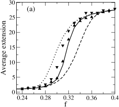
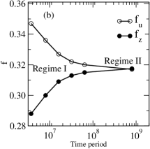
Figure 5: (a) The variation of the average extension as a function of force $f$. Dotted and dashed lines correspond to simple average of backward and forward paths, respectively. The weighted average of backward and forward paths are shown by up and down triangles, respectively. The solid line represents the equilibrium $f-y$ curve. (b) Simulated values of unzipping force ($f_{u}$) and rezipping force ($f_{z}$) as a function of time. Regime I corresponds to the non-equilibrium, where hysteresis has been seen hatch . Regime II corresponds to the equilibrium, where equilibrium response of DNA has been studied prentiss ; woodside .

In another study, Chattopadhyay and Marenduzzo chatto studied the dynamics of a polymer chain, whose ends are anchored. An oscillatory force was applied at the intermediate bead. They also observed hysteresis for the flexible polymer chain. However, they showed a crossover from a periodic limit cycle (hysteresis) to an aperiodic dynamics as the polymer gets stiffer. Since the unzipping experiments prentiss ; hatch usually are performed on a long chain (few Kbps) much greater than the persistence length of DNA, their model studies chatto also imply the existence of hysteresis under periodic force persistense .

Are the dynamic transition and the scaling proposed here observable in single molecule experiments? To answer this, in Fig. 5b, we show how the system approaches the equilibrium (regime II) from the non-equilibrium (regime I). This is in accordance with experiment followed by simulation hatch . For a two state model, time needed to cross the energy barrier $\Delta E(10-20k_{B}T)$ depending upon the length and sequence of DNA lies in between 4s to 15 min cocco . The equilibrium response of DNA unzipping (regime II) has been studied in experiments belong to this time scale prentiss ; woodside as we obtained in our simulation, but in ($\mu s$) range. There is a mismatch of the time scale because of the coarse grained description of the model. One of the possible ways to check the feasibility of the experiment from our simulation is to compare the ratio of time needed for the equilibrium (shown in Fig.2 by turquoise color) and the non-equilibrium regime (say black in Fig. 2). From our simulation, this ratio turns out to be $\sim$ 1000. If the experimental equilibrium time is 900 seconds prentiss then the lower limit of time is 900/1000 $\sim$ 1 second. Hence, by manipulating the amplitude and the frequency in the intermediate time scale (1s-15 minutes), it is possible to perform experiments where the dynamical transition may take place.

In conclusion, we have studied the response of a periodic force on DNA unzipping. We showed the existence of a dynamic transition, where by varying the frequency of the applied force, a dsDNA can go from the zipped/unzipped state to a new dynamic (hysteretic) state. The area of the hysteresis loop found to scale with the same exponents as of spin systems. The scaling exponents are found to be quite robust and independent of length rakesh and friction coefficient sm . We also showed that by using the work theorem, it is possible to extract the equilibrium properties of the system from the non-equilibrium data, which have potential application in single molecule force measurements. At this stage, additional theoretical and numerical investigations are needed to establish a connection between dynamical transition in the spin systems and a polymer under periodic force. Since, the role of hysteresis in biological processes remains unexplored territory, our work calls for further experiments on periodically driven DNA to explore such hitherto unknown dynamical phase transitions and related scaling.

We thank S. M. Bhattacharjee, Deepak Dhar, Sriram Ramaswamy and Madan Rao for many helpful discussions on the subject. We acknowledge the financial supports from the DST and CSIR, India. Generous computer supports from MPIPKS Dresden are gratefully acknowledged by authors.

Supplementary material
Here, we briefly describe the simulation details adopted in this study. The model includes a string of beads, each bead represents a base associated with sugar and phosphate groups. We consider a sequence in such a way that the first half of the chain is complementary to the other half. This gives the possibility of the formation of a dsdNA at low temperature km . The energy of the model system, we adopted, is defined as

$$E=\sum_{i=1}^{N-1}k(d_{i,i+1}-d_{0})^{2}+\sum_{i=1}^{N-2}\sum_{j>i+1}^{N}4(\frac{B}{d_{i,j}^{12}}-\frac{A_{ij}}{d_{i,j}^{6}}),$$ (4)

where $N(=32)$ is the number of beads. The distance between beads $d_{ij}$, is defined as $|\vec{r}_{i}-\vec{r}_{j}|$, where $\vec{r}_{i}$ and $\vec{r}_{j}$ denote the position of bead $i$ and $j$, respectively. In the Hamiltonian (Eq. 4), we use dimensionless distances and energy parameters. The harmonic (first) term with spring constant $k$ (=100) couples the adjacent beads along the chain. The remaining terms correspond to Lennard-Jones (LJ) potential.The first term of LJ potential takes care of the “excluded volume effect”, where we set $B=1$. We assign the base pairing interaction $A_{ij}=1$ for native contacts and 0 for non-native ones mishra . This choice corresponds to the Go model go . By native, we mean that the first base forms pair with the $N^{th}$ (last one) base only and second base with $(N-1)^{th}$ base and so on as shown in Fig.1. The parameter $d_{0}(=1.12)$ corresponds to the equilibrium distance in the harmonic potential, which is close to the equilibrium position of the average L-J potential. In the Hamiltonian (Eq. 4), we use dimensionless distances and energy parameters. We obtained the dynamics by using the following Langevin equation Allen ; Smith

$$m\frac{d^{2}r_{i}}{dt^{2}}=-{\zeta}\frac{dr_{i}}{dt}+F_{c}+\Gamma$$ (5)

where $m(=1)$ and $\zeta(=0.4)$ are the mass of a bead and friction coefficient, respectively. Here, $F_{c}$ is defined as $-\frac{dE}{dr}$ and the random force $\Gamma$ is a white noise Smith i.e., $<{\Gamma(t)\Gamma(t^{\prime})}>=2\zeta T\delta(t-t^{\prime})$. This keeps temperature constant throughout the simulation. The equation of motion is integrated using 6^th order predictor corrector algorithm with a time step $\delta t=0.025$ mishra .

Following relations may be used to convert dimensionless units to real units: $T=\frac{k_{B}T^{*}}{\epsilon}$, $t=(\frac{\epsilon}{m{\sigma}^{2}})^{1/2}t^{*}$, $r=\frac{r^{*}}{\sigma}$ Allen , where $T^{*}$, $t^{*}$, $r^{*}$ and $\epsilon$ are temperature, time, distance and energy in real units. $\sigma$ is the inter particle distance at which potential goes to zero. For example, if we set effective base pairing energy $\epsilon\sim 0.1$ eV, we get $T_{m}^{*}\approx 85$ ⁰C, which corresponds to $T_{m}=0.23$ in the reduced unit as reported in Ref mishra . It is consistent with the one obtained by OligoCalc Kibbe for the same sequence. Similarly, by setting the average molecular weight of each bead $\sim 308$ g/mol and $\sigma=5.17$ $\AA$, we get $t\approx 3.0$ $t^{*}$ ps. However, this conversion is not valid for the entire range of force and temperature arxiv .

I Dependence of loop area on the applied frequency and amplitude of force

The area under the loop is the measure of the energy dissipated over a cycle. At fixed $F$, as $\nu$ decreases, $A_{loop}$ increases (Fig. 6a). At some value of $\nu$, $A_{loop}$ is found to be maximum and then it approaches to zero. In Fig. 6b, we have depicted the plots of $A_{loop}$ with $F$ for different $\nu$. In this case also, $A_{loop}$ increases with $F$ and above a certain amplitude, it starts decreasing. However, one can observe here that $A_{loop}$ is the slow variant of $F$ and never approaches to zero for all $F$.

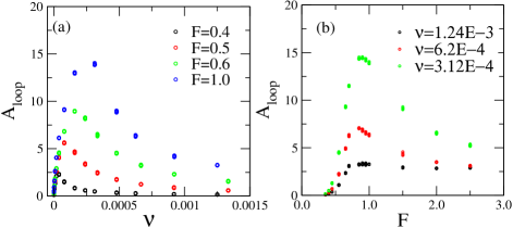
Figure 6: Variation of loop area $A_{loop}$ (a) with $\nu$ at different $F$, (b) with $F$ at different $\nu$.

II Dependence of scaling exponents on friction coefficient $\zeta$

We have checked our results for different values of $\zeta$. Here, we have shown results for 0.4 and 1.2. We found that the scaling exponents in high (Fig. 7) and low (Fig. 8) frequency regime, are independent of friction coefficient.

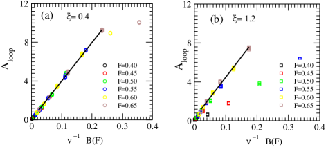
Figure 7: Loop area scales as $\nu^{-1}B(F)$ at high frequencies. Here, $B(F)\sim(F-f_{c})^{2\pm 0.1}$.

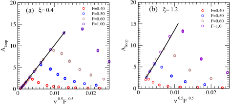
Figure 8: Loop area scales as $\nu^{0.5}F^{0.5}$ at low frequencies.

References

- (1) R. M. Wartell and A. S. Benight, Physics Reports 126, 67 (1985).
- (2) U. Bockelmann, B. Essevaz-Roulet, and F. Heslot, Phys. Rev. Lett. 79, 4489 (1997).
- (3) C. Danilowicz et al., Phys. Rev. Lett. 93, 078101 (2004).
- (4) S. M. Bhattacharjee, J. Phys. A 33, L423 (2000).
- (5) D. K. Lubensky and D. R. Nelson, Phys. Rev. Lett. 85, 1572 (2000).
- (6) Y. Kafri, D. Mukamel, and L. Peliti, Phys. Rev. Lett. 85, 4988 (2000).
- (7) D. Marenduzzo, S. M. Bhattacharjee, A. Maritan, E. Or- landini, and F. Seno, Phys. Rev. Lett. 88, 028102 (2002). 268, 319 (2007).
- (8) I. Donmez and S. S. Patel, Nucl. Acids Res. 34, 4216 (2006).
- (9) S. S. Velankar, P. Soultanas, M. S. Dillingham, H. S. Subramanya, and D. B. Wigley, Cell 97, 75 (1999).
- (10) M. E. Fairman-Williams and E. Jankowsky, J. Mol. Biol 415, 819 (2012).
- (11) D. S. Johnson et al Cell 129 1299 (2007).
- (12) A Basu, A J Schoeffler, J M Berger and Z Bryant Nat. Struc. & Mol. Bio. 19, 538 (2012).
- (13) N. Fili et al. NAR 38 4448 92010).
- (14) P Szymczak and H Janovjak, J. Mol.Biol. 390 443 (2009).
- (15) S. Kumar and M. S. Li, Phys. Rep. 486, 1 (2010).
- (16) J. F. Marko and E. Siggia, Macromolecules 28, 8759 (1995).
- (17) S. Kumar et al., Phys. Rev. Lett. 98, 128101 (2007).
- (18) G. Mishra, D. Giri, M. S. Li, and S. Kumar, J. Chem. Phys 135, 035102 (2011).
- (19) K. Hatch, C. Danilowicz, V. Coljee, and M. Prentiss, Phys. Rev E. 75, 051908 (2007).
- (20) R. Kapri, arXiv: 1201.3709 (2012).
- (21) M. Rao and R. Pandit, Phys. Rev. B 43, 3373 (1991).
- (22) M. Rao, H. R. Krishnamurthy, and R. Pandit, Phys. Rev. B 42, 856 (1990).
- (23) D. Dhar and P. Thomas, J. Phys. A 25, 4967 (1992).
- (24) B. K. Chakrabarti and M. Acharyya, Rev. Mod. Phys. 71, 847 (1999).
- (25) P. Sadhukhan and S. M. Bhattacharjee, J. Phys. A. 43, 245001 (2010).
- (26) See supplementary material for detail.
- (27) G. Mishra, P. Sadhukhan, S. M. Bhattacharjee, and S. Kumar, arxiv: 1204.2913 (2012).
- (28) For T = 0.1, critical force was found to be mishra .
- (29) Following relations may be used to convert dimensionless units to real units: , , Allen , where , , and are temperature, time, distance and energy in real units. is the inter particle distance at which potential goes to zero. For example, if we set effective base pairing energy eV, we get 0C, which corresponds to in the reduced unit as reported in Ref mishra . It is consistent with the one obtained by OligoCalc Kibbe for the same sequence. Similarly by setting, average molecular weight of each bead g/mol and , we get ps. However, this conversion does not work in the entire range of and arxiv .
- (30) M. P. Allen and D. J. Tildesley, Computer simulations of liquids (Oxford Science, 1987).
- (31) W. A. Kibbe, Nucl. Acids Res. 35, W43 (2007).
- (32) We have analyzed 80 conformations, but in Fig. 2, only 10 conformations are shown.
- (33) R. K. Mishra et al. to be published.
- (34) C. Jarzynski, Phys. Rev. Lett. 78, 2690 (1997).
- (35) P. Faccioli, A. Lonardi, and H. Orland, J. Chem. Phys. 133, 045104 (2010).
- (36) A. K. Chattopadhyay and D. Marenduzzo, Phys. Rev. Lett. 98, 088101 (2007).
- (37) Even in a realistic simulation which includes persistence length of dsDNA and ssDNA as well as helical structure in its description, one would expect hysteresis curve with no major change in the time scale (emerging from large energy gap) as reduction in entropy due to persistence length will be roughly compensated by the mobility DNA.
- (38) S. Cocco, Eur. Phys. J. E 10, 153 (2003).
- (39) M. T. Woodside et al., PNAS, 103, 6190 (2006).

References

- (1) S. Kumar and G. Mishra, Phys. Rev. E 78, 011907 (2008).
- (2) G. Mishra, D. Giri, M. S. Li, and S. Kumar, J. Chem. Phys 135, 035102 (2011).
- (3) N. Go and H. Abe, Biopolymers 20, 991 (1981).
- (4) M. P. Allen and D. J. Tildesley, Computer simulations of liquids (Oxford Science, 1987).
- (5) D. Frenkel and B. Smit, Understanding molecular simulation (Academic Press, London, 2002).
- (6) W. A. Kibbe, Nucl. Acids Res. 35, W43 (2007).
- (7) G. Mishra, P. Sadhukhan, S. M. Bhattacharjee, and S. Kumar, arxiv: 1204.2913 (2012).