Byzantine Consensus in Directed Graphs

Abstract

Consider a synchronous point-to-point network of $n$ nodes connected by directed links, wherein each node has a binary input. This paper proves a tight necessary and sufficient condition on the underlying communication topology for achieving Byzantine consensus among these nodes in the presence of up to $f$ Byzantine faults. We derive a necessary condition, and then we provide a constructive proof of sufficiency by presenting a Byzantine consensus algorithm for directed graphs that satisfy the necessary condition.

Prior work has developed analogous necessary and sufficient conditions for undirected graphs. It is known that, for undirected graphs, the following two conditions are together necessary and sufficient [8, 2, 6]: (i) $n\geq 3f+1$, and (ii) network connectivity greater than $2f$. However, these conditions are not adequate to completely characterize Byzantine consensus in directed graphs.

1 Introduction

In this work, we explore algorithms for achieving Byzantine consensus [9] in a synchronous point-to-point network in the presence of Byzantine faulty nodes. The network is modeled as a directed graph, i.e., the communication links between neighboring nodes are not necessarily bi-directional. Our work is motivated by the presence of directed links in wireless networks. However, we believe that the results here are of independent interest as well.

The Byzantine consensus problem [9] considers $n$ nodes, of which at most $f$ nodes may be faulty. The faulty nodes may deviate from the algorithm in arbitrary fashion. Each node has an input in $\{0,1\}$. A Byzantine consensus algorithm is correct if it satisfies the following three properties:

• Agreement: the output (i.e., decision) at all the fault-free nodes is identical.

• Validity: the output of every fault-free node equals the input of a fault-free node.

• Termination: every fault-free node eventually decides on an output.

In networks with undirected links (i.e., in undirected graphs), it is well-known that the following two conditions together are both necessary and sufficient for the existence of Byzantine consensus algorithms [8, 2, 6]: (i) $n\geq 3f+1$, and (ii) node connectivity greater than $2f$. The first condition, that is, $n\geq 3f+1$, is necessary for directed graphs as well. Under the second condition, each pair of nodes in the undirected graph can communicate reliably with each other. In particular, either a given pair of nodes is connected directly by an edge, or there are $2f+1$ node-disjoint paths between the pair of nodes. However, reliable communication between every pair of node is not necessary for achieving consensus in directed graphs. In Section 4.1, we address this statement in more details.

This paper presents tight necessary and sufficient conditions for Byzantine consensus in directed graphs. We provide a constructive proof of sufficiency by presenting a Byzantine consensus algorithm for directed graphs satisfying the necessary condition. The rest of the paper is organized as follows. Section 2 discusses the related work. Section 3 introduces our system model and some terminology used frequently in our presentation. The main result and the implications are presented in Section 4. The Byzantine consensus algorithm for directed graphs is described, and its correctness is also proved in Section 5. The paper summarizes in Section 6.

2 Related Work

Lamport, Shostak, and Pease addressed the Byzantine agreement problem in [9]. Subsequent work [8, 6] characterized the necessary and sufficient conditions under which the problem is solvable in undirected graphs. However, as noted above, these conditions are not adequate to fully characterize the directed graphs in which Byzantine consensus is feasible. In this work, we identify tight necessary and sufficient conditions for Byzantine consensus in directed graphs. The necessity proof presented in this paper is based on the state-machine approach, which was originally developed for conditions in undirected graphs [8, 6, 2]; however, due to the nature of directed links, our necessity proof is a non-trivial extension. The technique is also similar to the withholding mechanism, which was developed by Schmid, Weiss, and Keidar [12] to prove impossibility results and lower bounds for the number of nodes for synchronous consensus under transient link failures in fully-connected graphs; however, we do not assume the transient fault model as in [12], and thus, our argument is more straightforward.

In related work, Bansal et al. [3] identified tight conditions for achieving Byzantine consensus in undirected graphs using authentication. Bansal et al. discovered that all-pair reliable communication is not necessary to achieve consensus when using authentication. Our work differs from Bansal et al. in that our results apply in the absence of authentication or any other security primitives; also our results apply to directed graphs. We show that even in the absence of authentication all-pair reliable communication is not necessary for Byzantine consensus.

Several papers have also addressed communication between a single source-receiver pair. Dolev et al. [7] studied the problem of secure communication, which achieves both fault-tolerance and perfect secrecy between a single source-receiver pair in undirected graphs, in the presence of node and link failures. Desmedt and Wang considered the same problem in directed graphs [5]. In our work, we do not consider secrecy, and address the consensus problem rather than the single source-receiver pair problem. Shankar et al. [13] investigated reliable communication between a source-receiver pair in directed graphs allowing for an arbitrarily small error probability in the presence of a Byzantine failures. Our work addresses deterministically correct algorithms for consensus.

Our recent work [16, 14, 15] has considered a restricted class of iterative algorithms for achieving approximate Byzantine consensus in directed graphs, where fault-free nodes must agree on values that are approximately equal to each other using iterative algorithms with limited memory. The conditions developed in such prior work are not necessary when no such restrictions are imposed. Independently, LeBlanc et al. [11, 10], and Zhang and Sundaram [19, 18] have developed results for iterative algorithms for approximate consensus under a weaker fault model, where a faulty node must send identical messages to all the neighbors. In this work, we consider the problem of exact consensus (i.e., the outputs at fault-free nodes must be exactly identical), and we do not impose any restriction on the algorithms or faulty nodes.

Alchieri et al. [1] explored the problem of achieving exact consensus in unknown networks with Byzantine nodes, but the underlying communication graph is assumed to be fully-connected. In this work, the network is assumed to be known to all nodes, and may not be fully-connected.

3 System Model and Terminology

3.1 System Model

The system is assumed to be synchronous. The synchronous communication network consisting of $n$ nodes is modeled as a simple directed graph $G(\mathcal{V},\mathcal{E})$, where $\mathcal{V}$ is the set of $n$ nodes, and $\mathcal{E}$ is the set of directed edges between the nodes in $\mathcal{V}$. We assume that $n\geq 2$, since the consensus problem for $n=1$ is trivial. Node $i$ can transmit messages to another node $j$ if and only if the directed edge $(i,j)$ is in $\mathcal{E}$. Each node can send messages to itself as well; however, for convenience, we exclude self-loops from set $\mathcal{E}$. That is, $(i,i)\not\in\mathcal{E}$ for $i\in\mathcal{V}$. With a slight abuse of terminology, we will use the terms edge and link, and similarly the terms node and vertex, interchangeably.

All the communication links are reliable, FIFO (first-in first-out) and deliver each transmitted message exactly once. When node $i$ wants to send message M on link $(i,j)$ to node $j$, it puts the message M in a send buffer for link $(i,j)$. No further operations are needed at node $i$; the mechanisms for implementing reliable, FIFO and exactly-once semantics are transparent to the nodes. When a message is delivered on link ($i,j$), it becomes available to node $j$ in a receive buffer for link $(i,j)$. As stated earlier, the communication network is synchronous, and thus, each message sent on link ($i,j$) is delivered to node $j$ within a bounded interval of time.

Failure Model:

We consider the Byzantine failure model, with up to $f$ nodes becoming faulty. A faulty node may misbehave arbitrarily. Possible misbehavior includes sending incorrect and mismatching (or inconsistent) messages to different neighbors. The faulty nodes may potentially collaborate with each other. Moreover, the faulty nodes are assumed to have a complete knowledge of the execution of the algorithm, including the states of all the nodes, contents of messages the other nodes send to each other, the algorithm specification, and the network topology.

3.2 Terminology

We now describe terminology that is used frequently in our presentation. Upper case italic letters are used below to name subsets of ${\mathcal{V}}$, and lower case italic letters are used to name nodes in ${\mathcal{V}}$.

Incoming neighbors:

• Node $i$ is said to be an incoming neighbor of node $j$ if $(i,j)\in{\mathcal{E}}$.

• For set $B\subseteq{\mathcal{V}}$, node $i$ is said to be an incoming neighbor of set $B$ if $i\not\in B$, and there exists $j\in B$ such that $(i,j)\in{\mathcal{E}}$. Set $B$ is said to have $k$ incoming neighbors in set $A$ if set $A$ contains $k$ distinct incoming neighbors of $B$.

Directed paths:

All paths used in our discussion are directed paths.

• Paths from a node $i$ to another node $j$:

  • For a directed path from node $i$ to node $j$, node $i$ is said to be the “source node” for the path.

  • An “$(i,j)$-path” is a directed path from node $i$ to node $j$. An “$(i,j)$-path excluding $X$” is a directed path from node $i$ to node $j$ that does not contain any node from set $X$.

  • Two paths from node $i$ to node $j$ are said to be “disjoint” if the two paths only have nodes $i$ and $j$ in common, with all remaining nodes being distinct.

  • The phrase “$d$ disjoint $(i,j)$-paths” refers to $d$ pairwise disjoint paths from node $i$ to node $j$. The phrase “$d$ disjoint $(i,j)$-paths excluding $X$” refers to $d$ pairwise disjoint $(i,j)$-paths that do not contain any node from set $X$.

• Every node $i$ trivially has a path to itself. That is, for all $i\in{\mathcal{V}}$, an $(i,i)$-path excluding ${\mathcal{V}}-\{i\}$ exists.

• Paths from a set $S$ to node $j\not\in S$:

  • A path is said to be an “$(S,j)$-path” if it is an $(i,j)$-path for some $i\in S$. An “$(S,j)$-path excluding $X$” is a $(S,j)$-path that does not contain any node from set $X$.

  • Two $(S,j)$-paths are said to be “disjoint” if the two paths only have node $j$ in common, with all remaining nodes being distinct (including the source nodes on the paths).

  • The phrase “$d$ disjoint $(S,j)$-paths” refers to $d$ pairwise disjoint $(S,j)$-paths. The phrase “$d$ disjoint $(S,j)$-paths excluding $X$” refers to $d$ pairwise disjoint $(S,j)$-paths that do not contain any node from set $X$.

Graph Properties:

Definition 1

Given disjoint subsets $A,B,F$ of ${\mathcal{V}}$ such that $|F|\leq f$, set $A$ is said to propagate in ${\mathcal{V}}-F$ to set $B$ if either (i) $B=\emptyset$, or (ii) for each node $b\in B$, there exist at least $f+1$ disjoint $(A,b)$-paths excluding $F$.

We will denote the fact that set $A$ propagates in ${\mathcal{V}}-F$ to set $B$ by the notation

$$A\stackrel{{\scriptstyle{\mathcal{V}}-F}}{{\rightsquigarrow}}{B}$$

When it is not true that $A\stackrel{{\scriptstyle{\mathcal{V}}-F}}{{\rightsquigarrow}}{B}$, we will denote that fact by

$$A\stackrel{{\scriptstyle{\mathcal{V}}-F}}{{\not\rightsquigarrow}}{B}$$

For example, consider Figure 1 below when $f=2$ and $F=\{u_{1},u_{2}\},A=\{u_{3},u_{4},u_{5},u_{6},u_{7}\}$ and $B=\{w_{1},w_{2},w_{3},w_{4},w_{5},w_{6},w_{7}\}$, then $B\stackrel{{\scriptstyle{\mathcal{V}}-F}}{{\rightsquigarrow}}{A}$ and $A\stackrel{{\scriptstyle{\mathcal{V}}-F}}{{\not\rightsquigarrow}}{B}$.

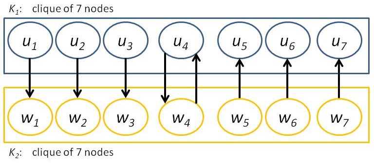
Figure 1: A network tolerating $2$ faults. Edges inside cliques $K_{1}$ and $K_{2}$ are not shown.

Definition 2

For $F\subset{\mathcal{V}}$, graph $G_{-F}$ is obtained by removing from $G({\mathcal{V}},{\mathcal{E}})$ all the nodes in $F$, and all the links incident on nodes in $F$.

Definition 3

A subgraph $S$ of $G$ is said to be strongly connected, if for all nodes $i,j$ in $S$, there exists an $(i,j)$-path in $G$.

4 Main Result

We now present the main result of this paper.

Theorem 1

Byzantine consensus is possible in $G(\mathcal{V},\mathcal{E})$ if and only if for any node partition $A,B,F$ of $\mathcal{V}$, where $A$ and $B$ are both non-empty, and $0\leq|F|\leq f$, either $A\stackrel{{\scriptstyle{\mathcal{V}}-F}}{{\rightsquigarrow}}{B}$ or $B\stackrel{{\scriptstyle{\mathcal{V}}-F}}{{\rightsquigarrow}}{A}$.

Proof:  Appendix A presents the proof of necessity of the condition in the theorem. In Appendix A, we first prove the necessity of an alternate form of the condition using the state-machine approach developed in prior work [8, 6, 2]. We then prove that the alternate necessary condition is equivalent to the condition stated in Theorem 1.

In Section 5, we present a constructive proof of sufficiency of the condition in the theorem. In particular, we present a Byzantine consensus algorithm and prove its correctness in all directed graphs that satisfy the condition stated in Theorem 1. $\Box$

4.1 Implications of the necessary and sufficient condition

Here, we discuss some interesting implications of Theorem 1.

• Lower bounds on number of nodes and incoming neighbors are identical to the case in undirected networks [8, 6, 2]:

  This observation is not surprising, since undirected graphs are a special case of directed graphs.

  Corollary 1

  Suppose that a correct Byzantine consensus algorithm exists for $G(\mathcal{V},\mathcal{E})$. Then, (i) $n\geq 3f+1$, and (ii) if $f>0$, then each node must have at least $2f+1$ incoming neighbors.

  Proof:  The proof is in Appendix C. $\Box$

• Reliable communication between all node pairs is not necessarily required:

  This observation is also not surprising, but nevertheless interesting (because, in undirected graphs, Byzantine consensus is feasible if and only if all node pairs can communicate with each other reliably). To illustrate the above observation, consider the simple example in Figure 2, with $f=1$. In Figure 2, nodes $v_{1},v_{2},v_{3},v_{4}$ have directed links to each other, forming a 4-node clique – the links inside the clique are not shown in the figure. Node $x$ does not have a directed link to any other node, but has links from the other 4 nodes. Yet, Byzantine consensus can be achieved easily by first reaching consensus within the 4-node clique, and then propagating the consensus value (for the 4-node consensus) to node $x$. Node $x$ can choose majority of the values received from the nodes in the 4-node clique as its own output. It should be easy to see that this algorithm works correctly for inputs in $\{0,1\}$ as required in the Byzantine consensus formulation considered in this work.

  

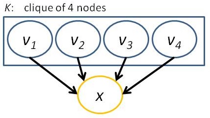
  Figure 2: A network tolerating $1$ fault. Edges inside clique $K$ are not shown.

• For a cut $(A,B)$ of the communication graph, there may not necessarily be $2f+1$ disjoint links in any one direction (i.e., from nodes in $A$ to nodes in $B$, or vice-versa):

  The above observation is surprising, since it suggests that reliable communication may not be feasible in either direction across a given cut in the communication graph. We illustrate this using the system in Figure 1 in Section 3, which contains two cliques $K_{1}$ and $K_{2}$, each containing 7 nodes. Within each clique, each node has a directed link to the other 6 nodes in that clique – these links are not shown in the figure. There are 8 directed links with one endpoint in clique $K_{1}$ and the other endpoint in clique $K_{2}$. We prove in Appendix B that Byzantine consensus can be achieved in this system with $f=2$. However, there are only 4 directed links from $K_{1}$ to $K_{2}$, and 4 directed links from $K_{2}$ to $K_{1}$. Thus, reliable communication is not guaranteed across the cut $(K_{1},K_{2})$ in either direction. Yet, Byzantine consensus is achievable using Algorithm BC. In Appendix B, we present a family of graphs, named 2-clique network, which satisfies the condition in Theorem 1. Figure 1 shown in Section 3 is the 2-clique network for $f=2$. Section 5 proves that Byzantine consensus is possible in all graphs that satisfy the necessary condition. Therefore, consensus is possible in the 2-clique network as well.

5 Sufficiency: Algorithm BC and Correctness Proof

In this section, we assume that graph $G({\mathcal{V}},{\mathcal{E}})$ satisfies the condition stated in Theorem 1, even if this is not stated explicitly again. We present Algorithm BC (Byzantine Consensus) and prove its correctness in all graphs that satisfy the condition in Theorem 1. This proves that the necessary condition is also sufficient. When $f=0$, all the nodes are fault-free, and as shown in Appendix E, the proof of sufficiency is trivial. In the rest of our discussion below, we will assume that $f>0$.

The proposed Algorithm BC is presented below. Each node $i$ maintains two state variables that are explicitly used in our algorithm: $v_{i}$ and $t_{i}$. Each node maintains other state as well (such as the routes to other nodes); however, we do not introduce additional notation for that for simplicity.

• Variable $v_{i}$: Initially, $v_{i}$ at any node $i$ is equal to the binary input at node $i$. During the execution of the algorithm, $v_{i}$ at node $i$ may be updated several times. Value $v_{i}$ at the end of the algorithm represents node $i$’s decision (or output) for Algorithm BC. The output at each node is either 0 or 1. At any time during the execution of the algorithm, the value $v_{i}$ at node $i$ is said to be valid, if it equals some fault-free node’s input. Initial value $v_{i}$ at a fault-free node $i$ is valid, because it equals its own input. Lemma 1 proved later in Section 5.4 implies that $v_{i}$ at a fault-free node $i$ always remains valid throughout the execution of Algorithm BC.

• Variable $t_{i}$: Variable $t_{i}$ at any node $i$ may take a value in $\{0,1,\perp\}$, where $\perp$ is distinguished from 0 and 1. Algorithm BC makes use of procedures Propagate and Equality that are described soon below. These procedures take $t_{i}$ as input, and possibly also modify $t_{i}$. Under some circumstances, as discussed later, state variable $v_{i}$ at node $i$ is set equal to $t_{i}$, in order to update $v_{i}$.

Algorithm BC consists of two loops, an OUTER loop, and an INNER loop. The OUTER loop is performed for each subset of nodes $F$, $|F|\leq f$. For each iteration of the OUTER loop, many iterations of the INNER loop are performed. The nodes in $F$ do not participate in any of these INNER loop iterations. For a chosen $F$, each iteration of the INNER loop is performed for a different partition of ${\mathcal{V}}-F$.

Since there are at most $f$ faults, one iteration of the OUTER loop has $F$ exactly equal to the set of faulty nodes. Denote the actual set of faulty nodes as $F^{*}$. Algorithm BC has two properties, as proved later:

• State $v_{i}$ of each fault-free node $i$ at the end of any particular INNER loop iteration equals the state of some fault-free node at the start of that INNER loop iteration. Thus, Algorithm BC ensures that the state $v_{i}$ of each fault-free node $i$ remains valid at all times.

• By the end of the OUTER loop iteration for $F=F^{*}$, all the fault-free nodes reach agreement.

The above two properties ensure that, when Algorithm BC terminates, the validity and agreement properties are both satisfied.

Each iteration of the INNER loop, for a given set $F$, considers a partition $A,B$ of the nodes in ${\mathcal{V}}-F$ such that $A\stackrel{{\scriptstyle{\mathcal{V}}-F}}{{\rightsquigarrow}}{B}$. Having chosen a partition $A,B$, intuitively speaking, the goal of the INNER loop iteration is for the nodes in set $A$ to attempt to influence the state of the nodes in the other partition. A suitable set $S\subseteq A\cup B$ is identified and agreed a priori using the known topology information. There are two possible cases. In Case 1 in Algorithm BC, $S\subseteq A$, and nodes in $S$ use procedure Equality (step (b) in the pseudo-code) to decide the value to propagate to nodes in ${\mathcal{V}}-F-S$ (step (c)). In Case 2, $S\subseteq A\cup B$, and nodes in $S$ first learn the states at nodes in $A$ using procedure Propagate (step (f)), and then use procedure Equality (step (g)) to decide the value to propagate to nodes in ${\mathcal{V}}-F-S$ (step (h)). These steps ensure that if $F=F^{*}$, and nodes in $A$ have the same $v$ value, then $S$ will propagate that value, and all nodes in ${\mathcal{V}}-F^{*}-S$ (Case 1: step (d)) or in ${\mathcal{V}}-F^{*}-(A\cap S)$ (Case 2: step (i)) will set $v$ value equal to the value propagated by $S$, and thus, the agreement is achieved. As proved later, in at least one INNER loop iteration with $F=F^{*}$, nodes in $A$ have the same $v$ value.

 

Algorithm BC

 

Comment: Note that Algorithm BC can be implemented distributedly if every node has prior knowledge of the topology. For the convenience of reader, the pseudo-code below is presented in a centralized fashion.

(OUTER LOOP)
For each $F\subset\mathcal{V}$, where $0\leq|F|\leq f$:

• (INNER LOOP)
  For each partition $A,B$ of ${\mathcal{V}}-F$ such that $A,B$ are non-empty, and $A\stackrel{{\scriptstyle{\mathcal{V}}-F}}{{\rightsquigarrow}}{B}$:

  STEP 1 of INNER loop:

  • Case 1: if $A\stackrel{{\scriptstyle{\mathcal{V}}-F}}{{\rightsquigarrow}}{B}$ and $B\stackrel{{\scriptstyle{\mathcal{V}}-F}}{{\not\rightsquigarrow}}{A}$:

    Choose a non-empty set $S\subseteq A$ such that $S\stackrel{{\scriptstyle{\mathcal{V}}-F}}{{\rightsquigarrow}}{{\mathcal{V}}-F-S}$, and $S$ is strongly connected in $G_{-F}$ ($G_{-F}$ is defined in Definition 2).

    • At each node $i\in S:~{}~{}~{}$ $t_{i}:=v_{i}$

    • Equality($S$)

    • Propagate($S,{\mathcal{V}}-F-S$)

    • At each node $j\in{\mathcal{V}}-F-S:~{}~{}~{}$ if $t_{j}\neq\perp$, then $v_{j}:=t_{j}$

  • Case 2: if $A\stackrel{{\scriptstyle{\mathcal{V}}-F}}{{\rightsquigarrow}}{B}$ and $B\stackrel{{\scriptstyle{\mathcal{V}}-F}}{{\rightsquigarrow}}{A}$:

    Choose a non-empty set $S\subseteq A\cup B$ such that $S\stackrel{{\scriptstyle{\mathcal{V}}-F}}{{\rightsquigarrow}}{{\mathcal{V}}-F-S}$, $S$ is strongly connected in $G_{-F}$, and $A\stackrel{{\scriptstyle{\mathcal{V}}-F}}{{\rightsquigarrow}}{(S-A)}$.

    • At each node $i\in A:~{}~{}~{}$ $t_{i}=v_{i}$

    • Propagate($A,S-A$)

    • Equality($S$)

    • Propagate($S,{\mathcal{V}}-F-S$)

    • At each node $j\in{\mathcal{V}}-F-(A\cap S):~{}~{}~{}$ if $t_{j}\neq\perp$, then $v_{j}:=t_{j}$

  STEP 2 of INNER loop:

  • Each node $k\in F$ receives $v_{j}$ from each $j\in N_{k}$, where $N_{k}$ is a set consisting of $f+1$ of $k$’s incoming neighbors in ${\mathcal{V}}-F$. If all the received values are identical, then $v_{k}$ is set equal to this identical value; else $v_{k}$ is unchanged.

 

5.1 Procedure Propagate($P,D$)

Propagate($P,D$) assumes that $P\subseteq{\mathcal{V}}-F$, $D\subseteq{\mathcal{V}}-F$, $P\cap D=\emptyset$ and $P\stackrel{{\scriptstyle{\mathcal{V}}-F}}{{\rightsquigarrow}}{D}$. Recall that set $F$ is the set chosen in each OUTER loop as specified by Algorithm BC.

  Propagate($P,D$)  

• Since $P\stackrel{{\scriptstyle{\mathcal{V}}-F}}{{\rightsquigarrow}}{D}$, for each $i\in D$, there exist at least $f+1$ disjoint ($P,i)$-paths that exclude $F$. The source node of each of these paths is in $P$. On each of $f+1$ such disjoint paths, the source node for that path, say $s$, sends $t_{s}$ to node $i$. Intermediate nodes on these paths forward received messages as necessary.

  When a node does not receive an expected message, the message content is assumed to be $\perp$.

• When any node $i\in D$ receives $f+1$ values along the $f+1$ disjoint paths above:
  if the $f+1$ values are all equal to 0, then $t_{i}:=0$; else if the $f+1$ values are all equal to 1, then $t_{i}:=1$; else $t_{i}:=\perp$. (Note that $:=$ denotes the assignment operator.)

For any node $j\not\in D$, $t_{j}$ is not modified during Propagate($P,D$). Also, for any node $k\in{\mathcal{V}}$, $v_{k}$ is not modified during Propagate($P,D$).

 

5.2 Procedure Equality($D$)

Equality($D$) assumes that $D\subseteq{\mathcal{V}}-F$, $D\neq\emptyset$, and for each pair of nodes $i,j\in D$, an $(i,j)$-path excluding $F$ exists, i.e., $D$ is strongly connected in $G_{-F}$ ($G_{-F}$ is defined in Definition 2).

  Equality($D$)  

• Each node $i\in D$ sends $t_{i}$ to all other nodes in $D$ along paths excluding $F$.

• Each node $j\in D$ thus receives messages from all nodes in $D$. Node $j$ checks whether values received from all the nodes in $D$ and its own $t_{j}$ are all equal, and also belong to $\{0,1\}$. If these conditions are not satisfied, then $t_{j}:=\perp$; otherwise $t_{j}$ is not modified.

For any node $k\not\in D$, $t_{k}$ is not modified in Equality($D$). Also, for any node $k\in{\mathcal{V}}$, $v_{k}$ is not modified in Equality($D$).

 

5.3 INNER Loop of Algorithm BC for $f>0$

Assume that $f>0$. For each $F$ chosen in the OUTER loop, the INNER loop of Algorithm BC examines each partition $A,B$ of ${\mathcal{V}}-F$ such that $A,B$ are both non-empty. From the condition in Theorem 1, we know that either $A\stackrel{{\scriptstyle{\mathcal{V}}-F}}{{\rightsquigarrow}}{B}$ or $B\stackrel{{\scriptstyle{\mathcal{V}}-F}}{{\rightsquigarrow}}{A}$. Therefore, with renaming of the sets we can ensure that $A\stackrel{{\scriptstyle{\mathcal{V}}-F}}{{\rightsquigarrow}}{B}$. Then, depending on the choice of $A,B,F$, two cases may occur: (Case 1) $A\stackrel{{\scriptstyle{\mathcal{V}}-F}}{{\rightsquigarrow}}{B}$ and $B\stackrel{{\scriptstyle{\mathcal{V}}-F}}{{\not\rightsquigarrow}}{A}$, and (Case 2) $A\stackrel{{\scriptstyle{\mathcal{V}}-F}}{{\rightsquigarrow}}{B}$ and $B\stackrel{{\scriptstyle{\mathcal{V}}-F}}{{\rightsquigarrow}}{A}$.

In Case 1 in the INNER loop of Algorithm BC, we need to find a non-empty set $S\subseteq A$ such that $S\stackrel{{\scriptstyle{\mathcal{V}}-F}}{{\rightsquigarrow}}{{\mathcal{V}}-F-S}$, and $S$ is strongly connected in $G_{-F}$ ($G_{-F}$ is defined in Definition 2). In Case 2, we need to find a non-empty set $S\subseteq A\cup B$ such that $S\stackrel{{\scriptstyle{\mathcal{V}}-F}}{{\rightsquigarrow}}{{\mathcal{V}}-F-S}$, $S$ is strongly connected in $G_{-F}$, and $A\stackrel{{\scriptstyle{\mathcal{V}}-F}}{{\rightsquigarrow}}{(S-A)}$. The following claim ensures that Algorithm BC can be executed correctly in $G$.

Claim 1

Suppose that $G({\mathcal{V}},{\mathcal{E}})$ satisfies the condition stated in Theorem 1. Then,

• The required set $S$ exists in both Case 1 and 2 of each INNER loop.

• Each node in set $F$ has enough incoming neighbors in ${\mathcal{V}}-F$ to perform step (j) of Algorithm BC with $f>0$.

Proof:  The proof of the first claim is proved in Appendix F.

Now, we prove the second claim. Consider nodes in set $F$. As shown in Corollary 1 in Section 4, when $f>0$, each node in ${\mathcal{V}}$ has at least $2f+1$ incoming neighbors. Since $|F|\leq f$, for each $k\in F$ there must exist at least $f+2$ incoming neighbors in ${\mathcal{V}}-F$. Thus, the desired set $N_{k}$ exists, satisfying the requirement in step (j) of Algorithm BC. $\Box$

5.4 Correctness of Algorithm BC for $f>0$

Recall that by assumption, $F^{*}$ is the actual set of faulty nodes in the network ($0\leq|F^{*}|\leq f$). Thus, the set of fault-free nodes is ${\mathcal{V}}-F^{*}$. When discussing a certain INNER loop iteration, we sometimes add superscripts start  and end  to $v_{i}$ for node $i$ to indicate whether we are referring to $v_{i}$ at the start, or at the end, of that INNER loop iteration, respectively. We first show that INNER loop preserves validity.

Lemma 1

For any given INNER loop iteration, for each fault-free node $j\in{\mathcal{V}}-F^{*}$, there exists a fault-free node $s\in{\mathcal{V}}-F^{*}$ such that $v_{j}^{\mbox{\it end}}=v_{s}^{\mbox{\it start}}$.

Proof:  To avoid cluttering the notation, for a set of nodes $X$, we use the phrase

a fault-free node $j\in X$

as being equivalent to

a fault-free node $j\in X-F^{*}$

because all the fault-free nodes in any set $X$ must also be in $X-F^{*}$.

Define set $Z$ as the set of values of $v_{i}$ at all fault-free $i\in{\mathcal{V}}$ at the start of the INNER loop iteration under consideration, i.e., $Z=\{v_{i}^{\mbox{\it start}}~{}|~{}i\in{\mathcal{V}}-F^{*}~{}\}$.

We first prove the claim in the lemma for the fault-free nodes in $\in{\mathcal{V}}-F$, and then for the fault-free nodes in $F$. Consider the following two cases in the INNER loop iteration.

• Case 1: $A\stackrel{{\scriptstyle{\mathcal{V}}-F}}{{\rightsquigarrow}}{B}$ and $B\stackrel{{\scriptstyle{\mathcal{V}}-F}}{{\not\rightsquigarrow}}{A}$:

  Observe that, in Case 1, $v_{i}$ remains unchanged for all fault-free $i\in S$. Thus, $v_{i}^{\mbox{\it end}}=v_{i}^{\mbox{\it start}}$ for $i\in S$, and hence, the claim of the lemma is trivially true for these nodes. We will now prove the claim for fault-free $j\in{\mathcal{V}}-F-S$.

  • step (a): Consider a fault-free node $i\in S$. At the end of step (a), $t_{i}$ is equal to $v_{i}^{\mbox{\it start}}$. Thus, $t_{i}\in Z$.

  • step (b): In step (b), step 2 of Equality($S$) either keeps $t_{i}$ unchanged at fault-free node $i\in S$ or modifies it to be $\perp$. Thus, now $t_{i}\in Z\cup\{\perp\}$.

  • step (c): Consider a fault-free node $j\in{\mathcal{V}}-F-S$. During Propagate($S,{\mathcal{V}}-F-S$), $j$ receives $f+1$ values along $f+1$ disjoint paths originating at nodes in $S$. Therefore, at least one of the $f+1$ values is received along a path that contains only fault-free nodes; suppose that the value received by node $j$ along this fault-free path is equal to $\alpha$. As observed above in step (b), $t_{i}$ at all fault-free nodes $i\in S$ is in $Z\cup\{\perp\}$. Thus, $\alpha\in Z\cup\{\perp\}$. Therefore, at fault-free node $j\in{\mathcal{V}}-F-S$, step 2 of Propagate($S,{\mathcal{V}}-F-S$) will result in $t_{j}\in\{\alpha,\perp\}\subseteq Z\cup\{\perp\}$.

  • step (d): Then it follows that, in step (d), at fault-free $j\in{\mathcal{V}}-F-S$, if $v_{j}$ is updated, then $v_{j}^{\mbox{\it end}}\in Z$. On the other hand, if $v_{j}$ is not updated, then $v_{j}^{\mbox{\it end}}=v_{j}^{\mbox{\it start}}\in Z$.

• Case 2: $A\stackrel{{\scriptstyle{\mathcal{V}}-F}}{{\rightsquigarrow}}{B}$ and $B\stackrel{{\scriptstyle{\mathcal{V}}-F}}{{\rightsquigarrow}}{A}$:

  Observe that, in Case 2, $v_{j}$ remains unchanged for all fault-free $j\in A\cap S$; thus $v_{j}^{\mbox{\it end}}=v_{j}^{\mbox{\it start}}$ for these nodes. Now, we prove the claim in the lemma for fault-free $j\in{\mathcal{V}}-F-(A\cap S)$.

  • step (e): For any fault-free node $i\in A$, at the end of step (e), $t_{i}\in Z$.

  • step (f): Consider a fault-free node $m\in S-A$. During Propagate($A,S-A$), $m$ receives $f+1$ values along $f+1$ disjoint paths originating at nodes in $A$. Therefore, at least one of the $f+1$ values is received along a path that contains only fault-free nodes; suppose that the value received by node $m$ along this fault-free path is equal to $\gamma\in Z$. Therefore, at node $m\in S-A$, Propagate($A,S-A$) will result in $t_{m}$ being set to a value in $\{\gamma,\perp\}\subseteq Z\cup\{\perp\}$. Now, for $m\in S\cap A$, $t_{m}$ is not modified in step (f), and therefore, for fault-free $m\in S\cap A$, $t_{m}\in Z$. Thus, we can conclude that, at the end of step (f), for all fault-free nodes $m\in S$, $t_{m}\in Z\cup\{\perp\}$.

  • step (g): In step (g), at each $m\in S$, Equality($S$) either keeps $t_{m}$ unchanged, or modifies it to be $\perp$. Thus, at the end of step (g), for all fault-free $m\in S$, $t_{m}$ remains in $Z\cup\{\perp\}$.

  • step (h): Consider a fault-free node $j\in{\mathcal{V}}-F-S$. During Propagate($S,{\mathcal{V}}-F-S$), $j$ receives $f+1$ values along $f+1$ disjoint paths originating at nodes in $S$. Therefore, at least one of the $f+1$ values is received along a path that contains only fault-free nodes; suppose that the value received by node $j$ along this fault-free path is equal to $\beta$. As observed above, after step (g), for each fault-free node $m\in S$, $t_{m}\in Z\cup\{\perp\}$. Therefore, $\beta\in Z\cup\{\perp\}$, and at node $j\in{\mathcal{V}}-F-S$, Propagate($S,{\mathcal{V}}-F-S$) will result in $t_{j}$ being set to a value in $\{\beta,\perp\}\subseteq Z\cup\{\perp\}$.

  • step (i): From the discussion of steps (g) and (h) above, it follows that, in step (i), if $v_{j}$ is updated at a fault-free $j\in{\mathcal{V}}-F-(S\cap A)$, then $v_{j}^{\mbox{\it end}}\in Z$; on the other hand, if $v_{j}$ is not modified, then $v_{j}^{\mbox{\it end}}=v_{j}^{\mbox{\it start}}\in Z$.

Now, consider a fault-free node $k\in F$. Step (j) uses set $N_{k}\subset{\mathcal{V}}-F$ such that $|N_{k}|=f+1$. As shown above, at the start of step (j), $v_{j}^{\mbox{\it end}}\in Z$ at all fault-free $j\in{\mathcal{V}}-F$. Since $|N_{k}|=f+1$, at least one of the nodes in $N_{k}$ is fault-free. Thus, of the $f+1$ values received by node $k$, at least one value must be in $Z$. It follows that if node $k$ changes $v_{k}$ in step (j), then the new value will also in $Z$; on the other hand, if node $k$ does not change $v_{k}$, then it remains equal to $v_{k}^{\mbox{\it start}}\in Z$. $\Box$

Lemma 2

Algorithm BC satisfies the validity property for Byzantine consensus.

Proof:  Recall that the state $v_{i}$ of a fault-free node $i$ is valid if it equals the input at a fault-free node. For each fault-free $i\in{\mathcal{V}}$, initially, $v_{i}$ is valid. Lemma 1 implies that after each INNER loop iteration, $v_{i}$ remains valid at each fault-free node $i$. Thus, when Algorithm BC terminates, $v_{i}$ at each fault-free node $i$ will satisfy the validity property for Byzantine consensus, as stated in Section 1. $\Box$

Lemma 3

Algorithm BC satisfies the termination property for Byzantine consensus.

Proof:  Recall that we are assuming a synchronous system, and the graph $G({\mathcal{V}},{\mathcal{E}})$ is finite. Thus, Algorithm BC performs a finite number of OUTER loop iterations, and a finite number of INNER loop iterations for each choice of $F$ in the OUTER loop, the number of iterations being a function of graph $G({\mathcal{V}},{\mathcal{E}})$. Hence, the termination property is satisfied. $\Box$

Lemma 4

Algorithm BC satisfies the agreement property for Byzantine consensus.

Proof Sketch: The complete proof is in Appendix G. Recall that $F^{*}$ denotes the actual set of faulty nodes in the network ($0\leq|F^{*}|\leq f$). Since the OUTER loop considers all possible $F\subset{\mathcal{V}}$ such that $|F|\leq f$, eventually, the OUTER loop will be performed with $F=F^{*}$. We will show that when OUTER loop is performed with $F=F^{*}$, agreement is achieved. After agreement is reached when $F=F^{*}$, Algorithm BC may perform the OUTER loop with other choices of set $F$. However, due to Lemma 1, the agreement among fault-free nodes is still preserved. (Also, due to Lemma 1, before the OUTER loop with $F=F^{*}$ is performed, $v_{i}$ at each fault-free node remains valid.)

Now, consider the OUTER loop with $F=F^{*}$. We will say that an INNER loop iteration with $F=F^{*}$ is “deciding” if one of the following conditions is true: (i) in Case 1 of the INNER loop iteration, after step (b) is performed, all the nodes in set $S$ have an identical value for variable $t$, or (ii) in Case 2 of the INNER loop iteration, after step (g) is performed, all the nodes in set $S$ have an identical value for variable $t$. As elaborated in Appendix G, when $F=F^{*}$, at least one of the INNER loop iterations must be a deciding iteration. Let us partition the INNER loop iterations when $F=F^{*}$ into three phases:

• Phase 1: INNER loop iterations before the first deciding iteration with $F=F^{*}$.

• Phase 2: The first deciding iteration with $F=F^{*}$.

• Phase 3: Remaining INNER loop iterations with $F=F^{*}$.

From the pseudo-code for Propagate and Equality, observe that when $F=F^{*}$, all paths used in the INNER loop iterations exclude $F=F^{*}$. That is, all these paths contain only fault-free nodes, since $F^{*}$ is the actual set of faulty nodes. In each INNER loop iteration in Phase 1, we can show that value $v_{i}$ for each fault-free node $i$ remains unchanged from previous INNER loop iteration. As elaborated in Appendix G, this together with fact that the value $v_{i}\in\{0,1\}$ for each fault-free node $i$, ensures that a deciding INNER loop iteration is eventually performed when $F=F^{*}$ (e.g., when set $A$ contains the fault-free nodes with $v$ value equal to $0$, and set $B$ contains the remaining fault-free nodes, or vice-versa). In Phase 2, Algorithm BC achieves agreement among fault-free nodes due to the fact that nodes in set $S$ reliably propagate an identical value to all the other nodes. Finally, in Phase 3, due to Lemma 1, agreement achieved in the previous phase is preserved. Therefore, at the end of the OUTER loop with $F=F^{*}$, agreement is achieved. $\Box$

Theorem 2

Algorithm BC satisfies the agreement, validity, and termination conditions.

Proof:  The theorem follows from Lemmas 2, 3 and 4. $\Box$

5.5 Application to Multi-Valued Consensus

Algorithm BC can be used to solve a particular version of multi-valued consensus with the following properties:

• Agreement: the output (i.e., decision) at all the fault-free nodes must be identical.

• Validity: If all fault-free nodes have the same input, then the output of every fault-free node equals its input.

• Termination: every fault-free node eventually decides on an output.

Under these conditions, if all the fault-free nodes do not have the same multi-valued input, then it is possible for the fault-free nodes to agree on a value that is not an input at any fault-free node. This multi-valued consensus problem for $L$-bit input values can be solved by executing $L$ instance of Algorithm BC, one instance for each bit of the input, on graphs that satisfy the condition stated in Theorem 1. The 1-bit output of each of the $L$ instances put together form the $L$-bit output of the multi-valued consensus problem. Correctness of this procedure follows from Theorem 2.

If the above validity condition for multi-valued consensus is made stronger, to require that the output value must be the multi-valued input of a fault-free node, then the condition in Theorem 1 is not sufficient for inputs that can take 3 or more distinct values.

6 Conclusion

For nodes with binary inputs, we present a tight necessary and sufficient condition for achieving Byzantine consensus in synchronous directed graphs. The condition is shown to be necessary using traditional state-machine approach [8, 6, 2]. Then, we provide a constructive proof of sufficiency by presenting a new Byzantine consensus algorithm for graphs satisfying the necessary condition. The algorithm can also be used to solve multi-valued consensus.

Two open problems are of further interest:

• Algorithm BC presented in Section 5 has exponential round complexity. The optimal round complexity for directed graphs is presently unknown.

• It is not known whether one can efficiently determine that a given graph satisfies the condition in Theorem 1 or not.

Appendices

Appendix A Necessity Proof of Theorem 1

This appendix presents the proof of necessity of the condition stated in Theorem 1. We first present an alternative form of the necessary condition, named Condition 1 below. We use the well-known state-machine approach [8, 6, 2] to show the necessity of Condition 1. Then, we prove that the condition stated in Theorem 1 is equivalent to Condition 1.

A.1 Necessary Condition 1

Necessary condition 1 is stated in Theorem 3 below. Its proof uses the familiar proof technique based on state machine approach. Although the proof of Theorem 3 is straightforward, we include it here for completeness. Readers may omit the proof of Theorem 3 in this section without lack of continuity.

We first define relations $\rightarrow$ and $\not\rightarrow$ that are used subsequently. These relations are defined for disjoint sets. Two sets are disjoint if their intersection is empty. For convenience of presentation, we adopt the convention that sets $A$ and $B$ are disjoint if either one of them is empty. More than two sets are disjoint if they are pairwise disjoint.

Definition 4

For disjoint sets of nodes $A$ and $B$, where $B$ is non-empty:

• $A\rightarrow B$ iff set $A$ contains at least $f+1$ distinct incoming neighbors of $B$.

  That is, $|~{}\{i~{}|~{}(i,j)\in{\mathcal{E}},~{}i\in A,~{}j\in B\}~{}|>f$.

• $A\not\rightarrow B$ iff $A\rightarrow B$ is not true.

The theorem below states Condition 1, and proves its necessity.

Theorem 3

Suppose that a correct Byzantine consensus algorithm exists for $G(\mathcal{V},\mathcal{E})$. For any partition $L,C,R,F$ of $\mathcal{V}$, such that both $L$ and $R$ are non-empty, and $|F|\leq f$, either $L\cup C\rightarrow R$, or $R\cup C\rightarrow L$.

We first describe the intuition behind the proof, followed by a formal proof. The proof is by contradiction.

Suppose that there exists a partition $L,C,R,F$ where $L,R$ are non-empty and $|F|\leq f$ such that $C\cup R\not\rightarrow L$, and $L\cup C\not\rightarrow R$. Assume that the nodes in $F$ are faulty, and the nodes in sets $L,C,R$ are fault-free. Note that fault-free nodes are not aware of the identity of the faulty nodes.

Consider the case when all the nodes in $L$ have input $m$, and all the nodes in $R\cup C$ have input $M$, where $m\neq M$. Suppose that the nodes in $F$ (if non-empty) behave to nodes in $L$ as if nodes in $R\cup C\cup F$ have input $m$, while behaving to nodes in $R$ as if nodes in $L\cup C\cup F$ have input $M$. This behavior by nodes in $F$ is possible, since the nodes in $F$ are all assumed to be faulty here.

Consider nodes in $L$. Let $N_{L}$ denote the set of incoming neighbors of $L$ in $R\cup C$. Since $R\cup C\not\rightarrow L$, $|N_{L}|\leq f$. Therefore, nodes in $L$ cannot distinguish between the following two scenarios: (i) all the nodes in $N_{L}$ (if non-empty) are faulty, rest of the nodes are fault-free, and all the fault-free nodes have input $m$, and (ii) all the nodes in $F$ (if non-empty) are faulty, rest of the nodes are fault-free, and fault-free nodes have input either $m$ or $M$. In the first scenario, for validity, the output at nodes in $L$ must be $m$. Therefore, in the second scenario as well, the output at the nodes in $L$ must be $m$. We can similarly show that the output at the nodes in $R$ must be $M$. Thus, if the condition in Theorem 3 is not satisfied, nodes in $L$ and $R$ can be forced to decide on distinct values, violating the agreement property. Now, we present the formal proof. Note that the formal proof relies on traditional state-machine approach [8, 2]. We include it here for completeness.

Proof of Theorem 3:

Proof:  The proof is by contradiction. Suppose that a correct Byzantine consensus algorithm, say ALGO, exists in $G({\mathcal{V}},{\mathcal{E}})$, and there exists a partition $F,L,C,R$ of ${\mathcal{V}}$ such that $C\cup R\not\rightarrow L$ and $L\cup C\not\rightarrow R$. Thus, $L$ has at most $f$ incoming neighbors in $R\cup C$, and $R$ has at most $f$ incoming neighbors in $L\cup C$. Let us define:

$$N_{L} = L R\cup C$$ set of incoming neighbors of in

$$N_{R} = R L\cup C$$ set of incoming neighbors of in

Then,

$$|N_{L}| \leq f$$ (1)

$$|N_{R}| \leq f$$ (2)

The behavior of each node $i\in{\mathcal{V}}$ when using ALGO can be modeled by a state machine that characterizes the behavior of each node $i\in{\mathcal{V}}$.

We construct a new network called ${\mathcal{N}}$, as illustrated in Figure 3. In ${\mathcal{N}}$, there are three copies of each node in $C$, and two copies of each node in $L\cup R\cup F$. In particular, C0 represents one copy of the nodes in $C$, C1 represents the second copy of the nodes in $C$, and C2 represents the third copy of the nodes in $C$. Similarly, R0 and R2 represent the two copies of the nodes in $R$, L0 and L1 represent the two copies of the nodes in $L$, and F1 and F2 represent the two copies of the nodes in $F$. Even though the figure shows just one vertex for C1, it represents all the nodes in $C$ (each node in $C$ has a counterpart in the nodes represented by C1). Same correspondence holds for other vertices in Figure 3.

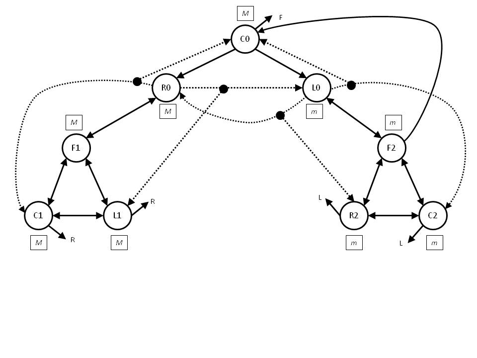
Figure 3: Network ${\mathcal{N}}$

The communication links in ${\mathcal{N}}$ are derived using the communication graph $G({\mathcal{V}},{\mathcal{E}})$. The figure shows solid edges and dotted edges, and also edges that do not terminate on one end. We describe all three types of edges below.

• Solid edges: If a node $i$ has a link to node $j$ in $G({\mathcal{V}},{\mathcal{E}})$, i.e., $(i,j)\in{\mathcal{E}}$, then each copy of node $j$ in ${\mathcal{N}}$ will have a link from one of the copies of node $i$ in ${\mathcal{N}}$. Exactly which copy of node $i$ has link to a copy of node $j$ is represented with the edges shown in Figure 3. For instance, the directed edge from vertex R0 to vertex F1 in Figure 3 indicates that, if for $r\in R$ and $k\in F$, link $(r,k)\in{\mathcal{E}}$, then there is a link in ${\mathcal{N}}$ from the copy of $r$ in R0 to the copy of $k$ in F1. Similarly, the directed edge from vertex F2 to vertex L0 in Figure 3 indicates that, if for $k\in F$ and $l\in L$, link $(k,l)\in{\mathcal{E}}$, then there is a link from the copy of $k$ in F2 to the copy of $l$ in L0. Other solid edges in Figure 3 represent other communication links in ${\mathcal{N}}$ similarly.

• Dotted edges: Dotted edges are defined similar to the solid edges, with the difference being that the dotted edges emulate a broadcast operation. Specifically, in certain cases, if link $(i,j)\in{\mathcal{E}}$, then one copy of node $i$ in ${\mathcal{N}}$ may have links to two copies of node $j$ in ${\mathcal{N}}$, with both copies of node $j$ receiving identical messages from the same copy of node $i$. This should be viewed as a “broadcast” operation that is being emulated unbeknownst to the nodes in ${\mathcal{N}}$. There are four such “broadcast edges” in the figure, shown as dotted edges. The broadcast edge from L0 to R0 and R2 indicates that if for $l\in L$ and $r\in R$, link $(l,r)\in{\mathcal{E}}$, then messages from the copy of node $l$ in L0 are broadcast to the copies of node $r$ in R0 and R2 both. Similarly, the broadcast edge from R0 to C0 and C1 indicates that if for $r\in R$ and $c\in C$, link $(r,c)\in{\mathcal{E}}$, then messages from the copy of node $r$ in R0 are broadcast to the copies of node $c$ in C0 and C1 both. There is also a broadcast edge from L0 to C0 and C2, and another broadcast edge from R0 to L0 and L1.

• “Hanging” edges: Five of the edges in Figure 3 do not terminate at any vertex. One such edge originates at each of the vertices C1, L1, R2, C2, and C0, and each such edge is labeled as R, L or F, as explained next. A hanging edge signifies that the corresponding transmissions are discarded silently without the knowledge of the sender. In particular, the hanging edge originating at L1 with label R indicates the following: if for $l\in L$ and $r\in R$, $(r,l)\in{\mathcal{E}}$, then transmissions by the copy of node $l$ in L1 to node $r$ are silently discarded without the knowledge of the copy of node $l$ in L1. Similarly, the hanging edge originating at C0 with label F indicates the following: if for $c\in C$ and $k\in F$, $(c,k)\in{\mathcal{E}}$, then transmissions by the copy of node $c$ in C0 to node $k$ are silently discarded without the knowledge of the copy of node $c$ in C0.

  It is possible to avoid using such “hanging” edges by introducing additional vertices in ${\mathcal{N}}$. We choose the above approach to make the representation more compact.

Whenever $(i,j)\in{\mathcal{E}}$, in network ${\mathcal{N}}$, each copy of node $j$ has an incoming edge from one copy of node $i$, as discussed above. The broadcast and hanging edges defined above are consistent with our communication model in Section 1. As noted there, each node, when sending a message, simply puts the message in the send buffer. Thus, it is possible for us to emulate hanging edges by discarding messages from the buffer, or broadcast edges by replicating the messages into two send buffers. (Nodes do not read messages in send buffers.)

Now, let us assign input of $m$ or $M$, where $m\neq M$, to each of the nodes in ${\mathcal{N}}$. The inputs are shown next to the vertices in small rectangles Figure 3. For instance, $M$ next to vertex C1 means that each node represented by C1 has input $M$ (recall that C1 represents one copy of each node in $C$). Similarly, $m$ next to vertex L0 means that each node represented by L0 has input $m$.

Let $\beta$ denote a particular execution of ALGO in ${\mathcal{N}}$ given the input specified above. Now, we identify three executions of ALGO in $G({\mathcal{V}},{\mathcal{E}})$ with a different set of nodes of size $\leq f$ behaving faulty. The behavior of the nodes is modeled by the corresponding nodes in ${\mathcal{N}}$.

• Execution $\alpha_{1}$:

  Consider an execution $\alpha_{1}$ of ALGO in $G({\mathcal{V}},{\mathcal{E}})$, where the incoming neighbors of nodes in $R$ that are in $L$ or $C$, i.e., nodes in $N_{R}$, are faulty, with the rest of the nodes being fault-free. In addition, all the fault-free nodes have inputs $M$. Now, we describe the behavior of each node.

  • The behavior of fault-free nodes in $R$, $F$, $C-N_{R}$ and $L-N_{R}$ is modeled by the corresponding nodes in R0, F1, C1, and L1 in ${\mathcal{N}}$. For example, nodes in $F$ send to their outgoing neighbors in $L$ the messages sent in $\beta$ by corresponding nodes in F1 to their outgoing neighbors in L1.

  • The behavior of the faulty nodes (i.e., nodes in $N_{R}$) is modeled by the behavior of the senders for the incoming links at the nodes in R0. In other words, faulty nodes are sending to their outgoing neighbors in $R$ the messages sent in $\beta$ by corresponding nodes in C0 or L0 to their outgoing neighbors in R0.

  Recall from (2) that $|N_{R}|\leq f$. Since ALGO is correct in $G({\mathcal{V}},{\mathcal{E}})$, the nodes in $R$ must agree on $M$, because all the fault-free nodes in network I have input $M$.

• Execution $\alpha_{2}$:

  Consider an execution $\alpha_{2}$ of ALGO in $G({\mathcal{V}},{\mathcal{E}})$, where the incoming neighbors of nodes in $L$ that are in $R$ or $C$, i.e., nodes in $N_{L}$, are faulty, with the rest of the nodes being fault-free. In addition, all the fault-free nodes have inputs $m$. Now, we describe the behavior of each node.

  • The behavior of fault-free nodes in $R-N_{L}$, $F$, $C-N_{L}$, and $L$ is modeled by the corresponding nodes in R2, F2, C2, and L0 in ${\mathcal{N}}$. For example, nodes in $F$ send to their outgoing neighbors in $R$ the messages sent in $\beta$ by corresponding nodes in F2 to their outgoing neighbors in R2.

  • The behavior of the faulty nodes (i.e., nodes in $N_{L}$) is modeled by the behavior of the senders for the incoming links at the nodes in L0. In other words, faulty nodes are sending to their outgoing neighbors in $L$ the messages sent in $\beta$ by corresponding nodes in C0 or R0 to their outgoing neighbors in L0.

  Recall from (1) that $|N_{L}|\leq f$. Since ALGO is correct in $G({\mathcal{V}},{\mathcal{E}})$, the nodes in $L$ must agree on $m$, because all the fault-free nodes in network II have input $m$.

• Execution $\alpha_{3}$:

  Consider an execution $\alpha_{3}$ of ALGO in $G({\mathcal{V}},{\mathcal{E}})$, where the nodes in F are faulty, with the rest of the nodes being fault-free. In addition, nodes in $R\cup C$ have inputs $M$, and the nodes in $L$ have inputs $m$. Now, we describe the behavior of each node.

  • The behavior of fault-free nodes in $R$, $C$ and $L$ is modeled by the corresponding nodes in R0, C0, and L0 in ${\mathcal{N}}$. For example, nodes in $R$ are sending to their outgoing neighbors in $L$ the messages sent in $\beta$ by corresponding nodes in R0 to their outgoing neighbors in L0.

  • The behavior of the faulty nodes (i.e., nodes in $F$) is modeled by the nodes in F1 and F2. In particular, faulty nodes in $F$ send to their outgoing neighbors in $R$ the messages sent in $\beta$ by corresponding nodes in F1 to their outgoing neighbors in R0. Similarly the faulty nodes in $F$ send to their outgoing neighbors in $L$ the messages sent in $\beta$ by corresponding nodes in F2 to their outgoing neighbors in L0.

  Then we make the following two observations regarding $\alpha_{3}$:

  • Nodes in $R$ must decide $M$ in $\alpha_{3}$ because, by construction, nodes in $R$ cannot distinguish between $\alpha_{1}$ and $\alpha_{3}$. Recall that nodes in $R$ decide on $M$ in $\alpha_{1}$.

  • Nodes in $L$ must decide $m$. because by construction, nodes in $L$ cannot distinguish between $\alpha_{2}$ and $\alpha_{3}$. Recall that nodes in $L$ decide on $m$ in $\alpha_{2}$.

  Thus, in $\alpha_{3}$, the fault-free nodes in $R$ and $L$ decide on different values, even though $|F|\leq f$. This violates the agreement condition, contradicting the assumption that ALGO is correct in $G({\mathcal{V}},{\mathcal{E}})$.

$\Box$

A.2 Equivalence of the Conditions Stated in Theorem 1 and Condition 1

In this section, we first prove that Condition 1 (the condition in Theorem 3) implies the condition in Theorem 1, and then prove that the condition in Theorem 1 implies Condition 1 (the condition in Theorem 3). Thus, the two conditions are proved to be equivalent. We first prove the two lemmas below. The proofs use the following version of Menger’s theorem [17].

Theorem 4 (Menger’s Theorem)

Given a graph $G(\mathcal{V},\mathcal{E})$ and two nodes $x,y\in{\mathcal{V}}$, then a set $S\subseteq{\mathcal{V}}-\{x,y\}$ is an $(x,y)$-cut if there is no $(x,y)$-path excluding $S$, i.e., every path from $x$ to $y$ must contain some nodes in $S$.

Lemma 5

Assume that Condition 1 (the condition in Theorem 3) holds for $G({\mathcal{V}},{\mathcal{E}})$. For any partition $A,B,F$ of $\mathcal{V}$, where $A$ is non-empty, and $|F|\leq f$, if $B\not\rightarrow A$, then $A\stackrel{{\scriptstyle{\mathcal{V}}-F}}{{\rightsquigarrow}}{B}$.

Proof:  Suppose that $A,B,F$ is a partition of ${\mathcal{V}}$, where $A$ is non-empty, $|F|\leq f$, and $B\not\rightarrow A$. If $B=\emptyset$, then by Definition 1, the lemma is trivially true. In the rest of this proof, assume that $B\neq\emptyset$.

Add a new (virtual) node $v$ to graph $G$, such that, (i) $v$ has no incoming edges, (ii) $v$ has an outgoing edge to each node in $A$, and (iii) $v$ has no outgoing edges to any node that is not in $A$. Let $G_{+v}$ denote the graph resulting after the addition of $v$ to $G({\mathcal{V}},{\mathcal{E}})$ as described above.

We want to prove that $A\stackrel{{\scriptstyle{\mathcal{V}}-F}}{{\rightsquigarrow}}{B}$. Equivalently, we want to prove that, in graph $G_{+v}$, for each $b\in B$, there exist $f+1$ disjoint ($v,b$)-paths excluding $F$. We will prove this claim by contradiction.

Suppose that $A\stackrel{{\scriptstyle{\mathcal{V}}-F}}{{\not\rightsquigarrow}}{B}$, and therefore, there exists a node $b\in B$ such that there are at most $f$ disjoint $(v,b)$ paths excluding $F$ in $G_{+v}$. By construction, there is no direct edge from $v$ to $b$. Then Menger’s theorem [17] implies that there exists a set $F_{1}\subseteq(A\cup B)-\{b\}$ with $|F_{1}|\leq f$, such that, in graph $G_{+v}$, there is no $(v,b)$-path excluding $F\cup F_{1}$. In other words, all $(v,b)$-paths excluding $F$ contain at least one node in $F_{1}$.

Let us define the following sets $L,R,C$. Some of the sets defined in this proof are illustrated in Figure 4.

• $L=A$.

  $L$ is non-empty, because $A$ is non-empty.

• $R~{}=~{}\{~{}i~{}|~{}i\in B-F_{1}~{}\mbox{and there exists an ($i,b$)-path excluding $F\cup F_{1}$}\}$.

  Thus, $R\subseteq B-F_{1}\subseteq B$.
  Note that $b\in R$. Thus, $R$ is non-empty.

• $C=B-R$.

  Thus, $C\subseteq B$. Since $R\subseteq B$, it follows that $R\cup C=B$.

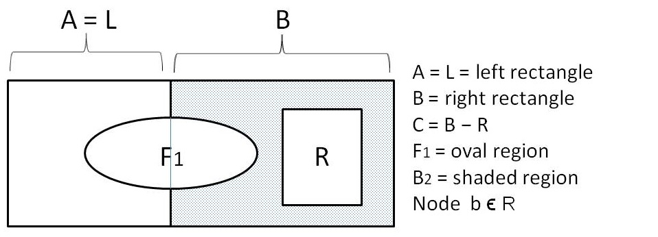
Figure 4: Illustration for the proof of Lemma 5

Observe that $L,R,C$ are disjoint sets, because $A$ and $B$ are disjoint, and $L\cup R\cup C=A\cup B$. Since set $F_{1}\subseteq A\cup B$, $L=A$, and $R\cap F_{1}=\emptyset$, we have $F_{1}\subseteq L\cup C$, and $F_{1}\cap B\subseteq C$. Thus, set $C$ can be partitioned into disjoint sets $B_{1}$ and $B_{2}$ such that

• $B_{1}=C\cap F_{1}=B\cap F_{1}\subseteq C\subseteq B$, and

• $B_{2}=C-B_{1}\subseteq C\subseteq B$. Note that $B_{2}\cap F_{1}=\emptyset$.

We make the following observations:

• For any $x\in A-F_{1}=L-F_{1}$ and $y\in R$, $(x,y)\not\in{\mathcal{E}}$.

  Justification: Recall that virtual node $v$ has a directed edge to $x$. If edge $(x,y)$ were to exist then there would be a $(v,b$)-path via nodes $x$ and $y$ excluding $F\cup F_{1}$ (recall from definition of $R$ that $y$ has a path to $b$ excluding $F\cup F_{1}$). This contradicts the definition of set $F_{1}$.

• For any $p\in B_{2}$, and $q\in R$, $(p,q)\not\in{\mathcal{E}}$.

  Justification: If edge $(p,q)$ were to exist, then there would be a $(p,b)$-path via node $q$ excluding $F\cup F_{1}$, since $q$ has a $(q,b)$-path excluding $F\cup F_{1}$. Then node $p$ should have been in $R$ by the definition of $R$. This is a contradiction to the assumption that $p\in B_{2}$, since $B_{2}\cap R\subseteq C\cap R=\emptyset$.

Thus, all the incoming neighbors of set $R$ are contained in $F\cup F_{1}$ (note that $F_{1}=(A\cap F_{1})\cup B_{1}$). Recall that $F_{1}\subseteq L\cup C$. Since $|F_{1}|\leq f$, it follows that

$$L\cup C\not\rightarrow R$$ (3)

Recall that $B\not\rightarrow A$. By definitions of $L,R,C$ above, we have $A=L$ and $B=C\cup R$. Thus,

$$C\cup R\not\rightarrow L$$ (4)

(3) and (4) contradict the condition in Theorem 3. Thus, we have proved that $A\stackrel{{\scriptstyle{\mathcal{V}}-F}}{{\rightsquigarrow}}{B}$. $\Box$

Lemma 6

Assume that Condition 1 (the condition in Theorem 3) holds for $G({\mathcal{V}},{\mathcal{E}})$. Consider a partition $A,B,F$ of $\mathcal{V}$, where $A,B$ are both non-empty, and $|F|\leq f$. If $B\stackrel{{\scriptstyle{\mathcal{V}}-F}}{{\not\rightsquigarrow}}{A}$ then there exist $A^{\prime}$ and $B^{\prime}$ such

• $A^{\prime}$ and $B^{\prime}$ are both non-empty,

• $A^{\prime}$ and $B^{\prime}$ form a partition of $A\cup B$,

• $A^{\prime}\subseteq A$ and $B\subseteq B^{\prime}$, and

• $B^{\prime}\not\rightarrow A^{\prime}$.

Proof:  Suppose that $B\stackrel{{\scriptstyle{\mathcal{V}}-F}}{{\not\rightsquigarrow}}{A}$.

Add a new (virtual) node $w$ to graph $G$, such that, (i) $w$ has no incoming edges, (ii) $w$ has an outgoing edge to each node in $B$, and (iii) $w$ has no outgoing edges to any node that is not in $B$. Let $G_{+w}$ denote the graph resulting after addition of $w$ to $G({\mathcal{V}},{\mathcal{E}})$ as described above.

Since $B\stackrel{{\scriptstyle{\mathcal{V}}-F}}{{\not\rightsquigarrow}}{A}$, for some node $a\in A$ there exist at most $f$ disjoint $(B,a)$-paths excluding $F$. Therefore, there exist at most $f$ disjoint $(w,a)$-paths excluding $F$ in $G_{+w}$. Also by construction, $(w,a)\not\in{\mathcal{E}}$. Then, by Menger’s theorem [17], there must exist $F_{1}\subseteq(A\cup B)-\{a\}$, $|F_{1}|\leq f$, such that, in graph $G_{+w}$, all ($w,a$)-paths excluding $F$ contain at least one node in $F_{1}$.

Define the following sets (also recall that ${\mathcal{V}}-F=A\cup B$):

• $L~{}=~{}\{~{}i~{}|~{}i\in{\mathcal{V}}-F-F_{1}~{}\mbox{and there exists an $(i,a)$-path excluding $F\cup F_{1}$}~{}\}.$

• $R~{}=~{}\{~{}j~{}|~{}j\in{\mathcal{V}}-F-F_{1}~{}\mbox{and there exists in $G_{+w}$ a $(w,j)$-path excluding $F\cup F_{1}$}~{}\}.$

  Set $R$ contains $B-F_{1}$ since all nodes in $B$ have edges from $w$.

• $C={\mathcal{V}}-F-L-R=(A\cup B)-L-R$.
  Observe that $F_{1}\subseteq C$ (because nodes of $F_{1}$ are not in $L\cup R$). Also, by definition of $C$, sets $C$ and $L\cup R$ are disjoint.

Observe the following:

• Sets $L$ and $R$ are disjoint, and set $L\subseteq A-F_{1}\subseteq A$. Also, $A\cup B=L\cup R\cup C$.

  Justification: $F_{1}\cap L=F_{1}\cap R=\emptyset$. By definition of $F_{1}$, all $(w,a)$-paths excluding $F$ contain at least one node in $F_{1}$. If $L\cap R$ were to be non-empty, we can find a $(w,a)$-path excluding $F\cup F_{1}$, which is a contradiction.

  Note that ${\mathcal{V}}-F-F_{1}=(A\cup B)-F_{1}$; therefore, $L\subseteq(A\cup B)-F_{1}$. $B-F_{1}\subseteq R$, since all nodes in $B-F_{1}$ have links from $w$. Since $L$ and $R$ are disjoint, it follows that $(B-F_{1})\cap L=\emptyset$, and therefore, $(A-F_{1})\cap L=L$; that is, $L\subseteq A-F_{1}\subseteq A$.

• For any $x\in C-F_{1}$ and $y\in L$, $(x,y)\not\in{\mathcal{E}}$.

  Justification: If such a link were to exist, then $x$ should be in $L$, which is a contradiction (since $C$ and $L$ are disjoint).

• There are no links from nodes in $R$ to nodes in $L$.

  Justification: If such a link were to exist, it would contradict the definition of $F_{1}$, since we can now find a $(w,a)$-path excluding $F\cup F_{1}$.

Thus, all the incoming neighbors of set $L$ must be contained in $F\cup F_{1}$. Recall that $F_{1}\subseteq C$ and $|F_{1}|\leq f$. Thus,

$$R\cup C\not\rightarrow L$$ (5)

Now define, $A^{\prime}=L$, $B^{\prime}=R\cup C$. Observe the following:

• $A^{\prime}$ and $B^{\prime}$ form a partition of $A\cup B$.

  Justification: $L,R,C$ are disjoint sets, therefore $A^{\prime}=L$ and $B^{\prime}=R\cup C$ are disjoint. By the definition of sets $L,R,C$ it follows that $A^{\prime}\cup B^{\prime}=L\cup(R\cup C)={\mathcal{V}}-F=A\cup B$.

• $A^{\prime}$ is non-empty and $A^{\prime}\subseteq A$.

  Justification: By definition of set $L$, set $L$ contains node $a$. Thus, $A^{\prime}=L$ is non-empty. We have already argued that $L\subseteq A$. Thus, $A^{\prime}\subseteq A$.

• $B^{\prime}$ is non-empty and $B\subseteq B^{\prime}$.

  Justification: Recall that $L,R,C$ are disjoint, and $L\cup R\cup C=A\cup B$. Thus, by definition of $C$, $R\cup C=(A\cup B)-L$. Since $L\subseteq A$, it follows that $B\subseteq R\cup C=B^{\prime}$. Also, since $B$ is non-empty, $B^{\prime}$ is also non-empty.

• $B^{\prime}\not\rightarrow A^{\prime}$

  Justification: Follows directly from (5), and the definition of $A^{\prime}$ and $B^{\prime}$.

This concludes the proof. $\Box$

Necessity Proof of Theorem 1

We now prove that Condition 1 (the condition in Theorem 3) implies the condition in Theorem 1.

Proof:

Assume that Condition 1 (the condition in Theorem 3) is satisfied by graph $G({\mathcal{V}},{\mathcal{E}})$. Consider a partition of $A,B,F$ of ${\mathcal{V}}$ such that $A,B$ are non-empty and $|F|\leq f$. Then, we must show that either $A\stackrel{{\scriptstyle{\mathcal{V}}-F}}{{\rightsquigarrow}}{B}$ or $B\stackrel{{\scriptstyle{\mathcal{V}}-F}}{{\rightsquigarrow}}{A}$.

Consider two possibilities:

• $B\stackrel{{\scriptstyle{\mathcal{V}}-F}}{{\rightsquigarrow}}{A}$: In this case, the proof is complete.

• $B\stackrel{{\scriptstyle{\mathcal{V}}-F}}{{\not\rightsquigarrow}}{A}$: Then by Lemma 6 in Appendix A, there exist non-empty sets $A^{\prime},B^{\prime}$ that form a partition of $A\cup B$ such that $A^{\prime}\subseteq A$, $B\subseteq B^{\prime}$, and $B^{\prime}\not\rightarrow A^{\prime}$. Lemma 5 in Appendix A then implies that $A^{\prime}\stackrel{{\scriptstyle{\mathcal{V}}-F}}{{\rightsquigarrow}}{B^{\prime}}$.

  Because $A^{\prime}\stackrel{{\scriptstyle{\mathcal{V}}-F}}{{\rightsquigarrow}}{B^{\prime}}$, for each $b\in B^{\prime}$, there exist $f+1$ disjoint $(A^{\prime},b)$-paths excluding $F$. Since $B\subseteq B^{\prime}$, it then follows that, for each $b\in B\subseteq B^{\prime}$, there exist $f+1$ disjoint $(A^{\prime},b)$-paths excluding $F$. Since $A^{\prime}\subseteq A$, and $F\cap A=\emptyset$, each $(A^{\prime},b)$-path excluding $F$ is also a $(A,b)$-path excluding $F$. Thus, for each $b\in B$, there exist $f+1$ disjoint $(A,b)$-paths excluding $F$. Therefore, $A\stackrel{{\scriptstyle{\mathcal{V}}-F}}{{\rightsquigarrow}}{B}$.

$\Box$

The proof above shows that the Condition 1 implies the condition in Theorem 1. That fact, and Lemma 7 below, together prove that the two forms of the condition are equivalent. Therefore, by Theorem 3, the condition in Theorem 1 is necessary.

Lemma 7

The condition stated in Theorem 1 implies the condition stated in Theorem 3 (i.e., Condition 1).

Proof:  We will prove the lemma by showing that, if Condition 1 is violated, then the condition stated in Theorem 1 is violated as well.

Suppose that the Condition 1 is violated. Then there exists a partition $L,C,R,F$ of ${\mathcal{V}}$ such that $L,R$ are both non-empty, $|F|\leq f$, $L\cup C\not\rightarrow R$ and $R\cup C\not\rightarrow L$.

Since $L\cup C\not\rightarrow R$, for any node $r\in R$, there exists a set $F_{r}$, $|F_{r}|\leq f$, such that all the $(L\cup C,r)$-paths excluding $F$ contain at least one node in $F_{r}$. Since $L\subseteq L\cup C$, Menger’s theorem [17] implies that there are at most $f$ disjoint $(L,r)$-paths excluding $F$. Thus, because $r\in R\cup C$, $L\stackrel{{\scriptstyle{\mathcal{V}}-F}}{{\not\rightsquigarrow}}{R\cup C}$.

Similarly, since $R\cup C\not\rightarrow L$, for any node $l\in L$, there exists a set $F_{l}$, $|F_{l}|\leq f$, such that all the $(R\cup C,l)$-paths excluding $F$ contain at least one node in $F_{l}$. Menger’s theorem [17] then implies that there are at most $f$ disjoint $(R\cup C,l)$-paths excluding $F$. Thus, $R\cup C\stackrel{{\scriptstyle{\mathcal{V}}-F}}{{\not\rightsquigarrow}}{L}$.

Define $A=L$, and $B=R\cup C$. Thus, $A,B,F$ is a partition of ${\mathcal{V}}$ such that $|F|\leq f$ and $A,B$ are non-empty. The two conditions derived above imply that $A\stackrel{{\scriptstyle{\mathcal{V}}-F}}{{\not\rightsquigarrow}}{B}$ and $B\stackrel{{\scriptstyle{\mathcal{V}}-F}}{{\not\rightsquigarrow}}{A}$, violating the condition stated in Theorem 1. $\Box$

Appendix B 2-clique Network

In this section, we present a family of graphs, namely 2-clique network. We will prove that the graph satisfies the necessary condition in Theorem 1, but each pair of nodes may not be able to communicate reliably with each other.

Definition 5

A graph $G({\mathcal{V}},{\mathcal{E}})$ consisting of $n=6f+2$ nodes, where $f$ is a positive even integer, is said to be a 2-clique network if all the following properties are satisfied:

• It includes two disjoint cliques, each consisting of $3f+1$ nodes. Suppose that the nodes in the two cliques are specified by sets $K_{1}$ and $K_{2}$, respectively, where $K_{1}=\{u_{1},u_{2},\cdots,u_{3f+1}\}\subset\mathcal{V}$, and $K_{2}=\mathcal{V}-K_{1}=\{w_{1},w_{2},\cdots,w_{3f+1}\}$. Thus, $(u_{i},u_{j})\in\mathcal{E}$ and $(w_{i},w_{j})\in\mathcal{E}$, for $1\leq i,j\leq 3f+1$ and $i\neq j$,

• $(u_{i},w_{i})\in\mathcal{E}$, for $1\leq i\leq\frac{3f}{2}$ and $i=3f+1$, and

• $(w_{i},u_{i})\in\mathcal{E}$, for $\frac{3f}{2}+1\leq i\leq 3f$ and $i=3f+1$.

Figure 1 is the 2-clique network for $f=2$. Note that Section 5 proves that Byzantine consensus is possible in all graphs that satisfy the necessary condition. Therefore, consensus is possible in the 2-clique network as well.

We first prove the following lemma for any graph $G({\mathcal{V}},{\mathcal{E}})$ that satisfies the necessary condition.

Lemma 8

Let $A,B,C,F$ be disjoint subsets of ${\mathcal{V}}$ such that $|F|\leq f$ and $A,B,C$ are non-empty. Suppose that $A\stackrel{{\scriptstyle{\mathcal{V}}-F}}{{\rightsquigarrow}}{B}$ and $A\cup B\stackrel{{\scriptstyle{\mathcal{V}}-F}}{{\rightsquigarrow}}{C}$. Then, $A\stackrel{{\scriptstyle{\mathcal{V}}-F}}{{\rightsquigarrow}}{B\cup C}$.

Proof:  The proof is by contradiction. Suppose that

• $A\stackrel{{\scriptstyle{\mathcal{V}}-F}}{{\rightsquigarrow}}{B}$,

• $A\cup B\stackrel{{\scriptstyle{\mathcal{V}}-F}}{{\rightsquigarrow}}{C}$, and

• $A\stackrel{{\scriptstyle{\mathcal{V}}-F}}{{\not\rightsquigarrow}}{B\cup C}$.

The first condition above implies that $|A|\geq f+1$. By Definition 1 and Menger’s Theorem [17], the third condition implies that there exists a node $v\in B\cup C$ and a set of nodes $P\subseteq{\mathcal{V}}-F-\{v\}$ such that $|P|\leq f$, and all $(A,v)$-paths excluding $F$ contain at least one node in $P$. In other words, there is no $(A,v)$-path excluding $F\cup P$. Observe that, because $A\stackrel{{\scriptstyle{\mathcal{V}}-F}}{{\rightsquigarrow}}{B}$, $v$ cannot be in $B$; therefore $v$ must belong to set $C$.

Let us define the sets $X$ and $Y$ as follows:

• Node $x\in X$ if and only if $x\in\mathcal{V}-F-P$ and there exists an $(A,x)$-path excluding $F\cup P$. It is possible that $P\cap A\neq\emptyset$; thus, the $(A,x)$-path cannot contain any nodes in $P\cap A$.

• Node $y\in Y$ if and only if $y\in\mathcal{V}-F-P$ and there exists an $(y,v)$-path excluding $F\cup P$.

By the definition of $X$ and $Y$, it follows that for any $x\in X,~{}y\in Y$, there cannot be any $(x,y)$-path excluding $F\cup P$. Also, since $A\stackrel{{\scriptstyle\mathcal{V}-F}}{{\rightsquigarrow}}{B}$, for each $b\in B-P$, there must exist an $(A,b)$-path excluding $F\cup P$; thus, $B-P\subseteq X$, and $B\subseteq X\cup P$. Similarly, $A\subseteq X\cup P$, and therefore, $A\cup B\subseteq X\cup P$.

By definition of $X$, there are no $(X\cup P,v)$-paths excluding $F\cup P$. Therefore, because $A\cup B\subseteq X\cup P$, there are no $(A\cup B,v)$-paths excluding $F\cup P$. Therefore, since $v\in C$, $A\cup B\stackrel{{\scriptstyle\mathcal{V}-F}}{{\not\rightsquigarrow}}{C}$. This is a contradiction to the second condition above. $\Box$

Now, we use Lemma 8 to prove the following Lemma.

Lemma 9

Suppose that $G(\mathcal{V},\mathcal{E})$ is a 2-clique network. Then graph $G$ satisfies the condition in Theorem 1.

Proof:

Consider a partition $A,B,F$ of ${\mathcal{V}}$, where $A$ and $B$ are both non-empty, and $|F|\leq f$. Recall from Definition 5 that $K_{1},K_{2}$ also form a partition of ${\mathcal{V}}$.

Define $A_{1}=A\cap K_{1},A_{2}=A\cap K_{2},B_{1}=B\cap K_{1},B_{2}=B\cap K_{2},F_{1}=F\cap K_{1}$ and $F_{2}=F\cap K_{2}$.

Define $\mathcal{E}^{\prime}$ to be the set of directed links from the nodes in $K_{1}$ to the nodes in $K_{2}$, or vice-versa. Thus, there are $\frac{3f}{2}+1$ directed links in $\mathcal{E}^{\prime}$ from the nodes in $K_{1}$ to the nodes in $K_{2}$, and the same number of links from the nodes in $K_{2}$ to the nodes in $K_{1}$. Each pair of links in $\mathcal{E}^{\prime}$, with the exception of the link pair between $a_{3f+1}$ and $b_{3f+1}$, is node disjoint. Since $|F|\leq f$, it should be easy to see that, at least one of the two conditions below is true:

• (a) There are at least $f+1$ directed links from the nodes in $K_{1}-F$ to the nodes in $K_{2}-F$.

• (b) There are at least $f+1$ directed links from the nodes in $K_{2}-F$ to nodes the in $K_{1}-F$.

Without loss of generality, suppose that condition (a) is true. Therefore, since $|K_{1}-F|\geq 2f+1$ and the nodes in $K_{2}-F$ form a clique, it follows that $K_{1}-F\stackrel{{\scriptstyle{\mathcal{V}}-F}}{{\rightsquigarrow}}{K_{2}-F}$. Then, because $K_{1}-F=A_{1}\cup B_{1}$ and $K_{2}-F=A_{2}\cup B_{2}$, we have

$$A_{1}\cup B_{1}\stackrel{{\scriptstyle\mathcal{V}-F}}{{\rightsquigarrow}}{A_{2}\cup B_{2}}.$$ (6)

$|K_{1}-F|\geq 2f+1$ also implies that either $|A_{1}|\geq f+1$ or $|B_{1}|\geq f+1$. Without loss of generality, suppose that $|A_{1}|\geq f+1$. Then, since the nodes in $A_{1}\cup B_{1}$ form a clique, it follows that $A_{1}\stackrel{{\scriptstyle\mathcal{V}-F_{1}-K_{2}}}{{\rightsquigarrow}}{B_{1}}$ (recall that $\mathcal{V}-F_{1}-K_{2}=A_{1}\cup B_{1}$). Since $\mathcal{V}-F_{1}-K_{2}\subset\mathcal{V}-F$, we have

$$A_{1}\stackrel{{\scriptstyle\mathcal{V}-F}}{{\rightsquigarrow}}{B_{1}}$$ (7)

(6) and (7), along with Lemma 8 above imply that $A_{1}\stackrel{{\scriptstyle{\mathcal{V}}-F}}{{\rightsquigarrow}}{B_{1}\cup A_{2}\cup B_{2}}$. Therefore, $A_{1}\stackrel{{\scriptstyle{\mathcal{V}}-F}}{{\rightsquigarrow}}{B_{1}\cup B_{2}}$, and $A_{1}\cup A_{2}\stackrel{{\scriptstyle{\mathcal{V}}-F}}{{\rightsquigarrow}}{B_{1}\cup B_{2}}$. Since $A=A_{1}\cup A_{2}$ and $B=B_{1}\cup B_{2}$, $A\stackrel{{\scriptstyle{\mathcal{V}}-F}}{{\rightsquigarrow}}{B}$. $\Box$

Appendix C Proof of Corollary 1

Proof:  Since $n\geq 3f+1$ is a necessary condition for Byzantine consensus in undirected graphs [8, 2], it follows that $n\geq 3f+1$ is also necessary for directed graphs. As presented below, this necessary condition can also be derived from Theorem 1.

For $f=0$, condition (i) in the corollary is trivially true. Now consider $f>0$. The proof is by contradiction. Suppose that $n\leq 3f$. As stated in Section 1, we assume $n\geq 2$, since consensus for $n=1$ is trivial. Partition ${\mathcal{V}}$ into three subsets $A,B,F$ such that $|F|\leq f$, $0<|A|\leq f$, and $0<|B|\leq f$. Such a partition can be found because $2\leq|{\mathcal{V}}|\leq 3f$. Since $A,B$ are both non-empty, and contain at most $f$ nodes each, we have $A\stackrel{{\scriptstyle{\mathcal{V}}-F}}{{\not\rightsquigarrow}}{B}$ and $B\stackrel{{\scriptstyle{\mathcal{V}}-F}}{{\not\rightsquigarrow}}{A}$, violating the condition in Theorem 1. Thus, $n\geq 3f+1$ is a necessary condition.

Now, for $f>0$, we show that it is necessary for each node to have at least $2f+1$ incoming neighbors. The proof is by contradiction. Suppose that for some node $i\in{\mathcal{V}}$, the number of incoming neighbors is at most $2f$. Partition ${\mathcal{V}}-\{i\}$ into two sets $L$ and $F$ such that $L$ is non-empty and contains at most $f$ incoming neighbors of $i$, and $|F|\leq f$. It should be easy to see that such $L,F$ can be found, since node $i$ has at most $2f$ incoming neighbors.

Define $A=\{i\}$ and $B={\mathcal{V}}-A-F=L$. Thus, $A,B,F$ form a partition of ${\mathcal{V}}$. Then, since $f>0$ and $|A|=1,|B|=|L|>0$, it follows that $A\stackrel{{\scriptstyle{\mathcal{V}}-F}}{{\not\rightsquigarrow}}{B}$. Also, since $B$ contains at most $f$ incoming neighbors of node $i$, and set $A$ contains only node $i$, there are at most $f$ node-disjoint $(B,i)$-paths. Thus, $B\stackrel{{\scriptstyle{\mathcal{V}}-F}}{{\not\rightsquigarrow}}{A}$. The above two conditions violate the necessary condition stated in Theorem 1. $\Box$

Appendix D Source Component

We introduce some definitions and results that are useful in the other appendices.

Definition 6

Graph decomposition: Let $H$ be a subgraph of $G({\mathcal{V}},{\mathcal{E}})$. Partition graph $H$ into non-empty strongly connected components, $H_{1},H_{2},\cdots,H_{h}$, where $h$ is a non-zero integer dependent on graph $H$, such that nodes $i,j\in H_{k}$ if and only if there exist $(i,j)$- and $(j,i)$-paths both excluding nodes outside $H_{k}$.

Construct a graph $H^{d}$ wherein each strongly connected component $H_{k}$ above is represented by vertex $c_{k}$, and there is an edge from vertex $c_{k}$ to vertex $c_{l}$ if and only if the nodes in $H_{k}$ have directed paths in $H$ to the nodes in $H_{l}$.

It is known that the decomposition graph $H^{d}$ is a directed acyclic graph [4].

Definition 7

Source component: Let $H$ be a directed graph, and let $H^{d}$ be its decomposition as per Definition 6. Strongly connected component $H_{k}$ of $H$ is said to be a source component if the corresponding vertex $c_{k}$ in $H^{d}$ is not reachable from any other vertex in $H^{d}$.

Definition 8

Reduced Graph: For a given graph $G(\mathcal{V},\mathcal{E})$, and sets $F\subset\mathcal{V}$, $F_{1}\subset{\mathcal{V}}-F$, such that $|F|\leq f$ and $|F_{1}|\leq f$, reduced graph $G_{F,F_{1}}(\mathcal{V}_{F,F_{1}},\mathcal{E}_{F,F_{1}})$ is defined as follows: (i) $\mathcal{V}_{F,F_{1}}=\mathcal{V}-F$, and (ii) $\mathcal{E}_{F,F_{1}}$ is obtained by removing from $\mathcal{E}$ all the links incident on the nodes in $F$, and all the outgoing links from nodes in $F_{1}$. That is, ${\mathcal{E}}_{F,F_{1}}={\mathcal{E}}-\{(i,j)~{}|~{}i\in F~{}~{}\mbox{or}~{}~{}j\in F\}-\{(i,j)~{}|~{}i\in F_{1}\}$.

Corollary 2

Suppose that graph $G(\mathcal{V},\mathcal{E})$ satisfies the condition stated in Theorem 3. For any $F\subset\mathcal{V}$ and $F_{1}\subset{\mathcal{V}}-F$, such that $|F|\leq f$ and $|F_{1}|\leq f$, let $S$ denote the set of nodes in the source component of $G_{F,F_{1}}$. Then, $S\stackrel{{\scriptstyle{\mathcal{V}}-F}}{{\rightsquigarrow}}{{\mathcal{V}}-F-S}$.

Proof:  Since $G_{F,F_{1}}$ contains non-zero number of nodes, its source component $S$ must be non-empty. If ${\mathcal{V}}-F-S$ is empty, then the corollary follows trivially by Definition 1. Suppose that ${\mathcal{V}}-F-S$ is non-empty. Since $S$ is a source component in $G_{F,F_{1}}$, it has no incoming neighbors in $G_{F,F_{1}}$; therefore, all of the incoming neighbors of $S$ in ${\mathcal{V}}-F$ in graph $G({\mathcal{V}},{\mathcal{E}})$ must belong to $F_{1}$. Since $|F_{1}|\leq f$, we have,

$$(\mathcal{V}-S-F)\not\rightarrow S$$

Lemma 5 in Appendix A then implies that

$$S\stackrel{{\scriptstyle{\mathcal{V}}-F}}{{\rightsquigarrow}}{{\mathcal{V}}-F-S}$$

$\Box$

Lemma 10

For any $F\subset{\mathcal{V}}$, $F_{1}\subset{\mathcal{V}}-F$, such that $|F|\leq f$, $|F_{1}|\leq f$:

• The source component of $G_{F,F_{1}}$ is strongly connected in $G_{-F}$. ($G_{-F}$ is defined in Definition 2 in Section 5.)

• The source component of $G_{F,F_{1}}$ does not contain any nodes in $F_{1}$.

Proof:  By Definition 6, each pair of nodes $i,j$ in the source component of graph $G_{F,F_{1}}$ has at least one $(i,j)$-path and at least one $(j,i)$-path consisting of nodes only in $G_{F,F_{1}}$, i.e., excluding nodes in $F$.

Since $F_{1}\subset{\mathcal{V}}-F$, $G_{F,F_{1}}$ contains other nodes besides $F_{1}$. Although nodes of $F_{1}$ belong to graph $G_{F,F_{1}}$, the nodes in $F_{1}$ do not have any outgoing links in $G_{F,F_{1}}$. Thus, a node in $F_{1}$ cannot have paths to any other node in $G_{F,F_{1}}$. Then, due to the connetedness requirement of a source component, it follows that no nodes of $F_{1}$ can be in the source component. $\Box$

Appendix E Sufficiency for $f=0$

The proof below uses the terminologies and results presented in Appendix D. We now prove that, when $f=0$, the necessary condition in Theorem 1 is sufficient to achieve consensus.

Proof:

When $f=0$, suppose that the graph $G$ satisfies the necessary condition in Theorem 1. Consider the source component $S$ in reduced graph $G_{\emptyset,\emptyset}=G$, i.e., in the reduced graph where $F=F_{1}=\emptyset$, as per Definition 8 in Appendix D. Note that by definition, $S$ is non-empty. Pick a node $i$ in the source component. By Lemma 10 in Appendix D, $S$ is strongly connected in $G$, and thus $i$ has a directed path to each of the nodes in $S$. By Corollary 2 in Appendix D, because $F=\emptyset$, $S\stackrel{{\scriptstyle{\mathcal{V}}}}{{\rightsquigarrow}}{{\mathcal{V}}-S}$, i.e., for each node $j\in{\mathcal{V}}-S$, an $(S,j)$-path exists. Since $S$ is strongly connected, an $(i,j)$-path also exists. Then consensus can be achieved simply by node $i$ routing its input to all the other nodes, and requiring all the nodes to adopt node $i$’s input as the output (or decision) for the consensus. It should be easy to see that termination, validity and agreement properties are all satisfied.

$\Box$

Appendix F Proof of Claim 1 in Section 5.3

The proof below uses the terminologies and results presented in Appendix D. We first prove a simple lemma.

Lemma 11

Given a partition $A,B,F$ of ${\mathcal{V}}$ such that $B$ is non-empty, and $|F|\leq f$, if $A\stackrel{{\scriptstyle{\mathcal{V}}-F}}{{\rightsquigarrow}}{B}$, then size of $A$ must be at least $f+1$.

Proof:  By definition, there must be at least $f+1$ disjoint $(A,b)$-paths excluding $F$ for each $b\in B$. Each of these $f+1$ disjoint paths will have a distinct source node in $A$. Therefore, such $f+1$ disjoint paths can only exist if $A$ contains at least $f+1$ distinct nodes. $\Box$

We now prove the claim (i) in Section 5.3.

Proof of Claim 1 in Section 5.3:

The second claim of Claim 1 is proved in the main body already. Now, we present the proof of the first claim:

The required set $S$ exists in both Case 1 and 2 of each INNER loop.

Consider the two cases in the INNER loop.

• Case 1:  $A\stackrel{{\scriptstyle{\mathcal{V}}-F}}{{\rightsquigarrow}}{B}$ and $B\stackrel{{\scriptstyle{\mathcal{V}}-F}}{{\not\rightsquigarrow}}{A}$:

  Since $B\stackrel{{\scriptstyle{\mathcal{V}}-F}}{{\not\rightsquigarrow}}{A}$, by Lemma 6 in Appendix A, there exist non-empty sets $A^{\prime},B^{\prime}$ that form a partition of $A\cup B={\mathcal{V}}-F$ such that $A^{\prime}\subseteq A$ and

  $$B^{\prime}\not\rightarrow A^{\prime}$$

  Let $F_{1}$ be the set of incoming neighbors of $A^{\prime}$ in $B^{\prime}$. Since $B^{\prime}\not\rightarrow A^{\prime}$, $|F_{1}|\leq f$. Then $A^{\prime}$ has no incoming neighbors in $G_{F,F_{1}}$. Therefore, the source component of $G_{F,F_{1}}$ must be contained within $A^{\prime}$. (The definition of source component is in Appendix D.) Let $S$ denote the set of nodes in this source component. Since $S$ is the source component, by Corollary 2 in Appendix D,

  $$S\stackrel{{\scriptstyle{\mathcal{V}}-F}}{{\rightsquigarrow}}{{\mathcal{V}}-S-F}.$$

  Since $S\subseteq A^{\prime}$ and $A^{\prime}\subseteq A$, $S\subseteq A$. Then, $B\subseteq(A\cup B)-S={\mathcal{V}}-S-F$; therefore, ${\mathcal{V}}-S-F$ is non-empty. Also, since $S\stackrel{{\scriptstyle{\mathcal{V}}-F}}{{\rightsquigarrow}}{{\mathcal{V}}-S-F}$, set $S$ must be non-empty (by Lemma 11 above). By Lemma 10 in Appendix D, $S$ is strongly connected in $G_{-F}$. (The definition of $G_{-F}$ is in Section 5.) Thus, set $S$ as required in Case 1 exists.

• Case 2:  $A\stackrel{{\scriptstyle{\mathcal{V}}-F}}{{\rightsquigarrow}}{B}$ and $B\stackrel{{\scriptstyle{\mathcal{V}}-F}}{{\rightsquigarrow}}{A}$:

  Recall that we consider $f>0$ in Section 5.3.

  By Corollary 1 in Section 4, since $|{\mathcal{V}}|=n>3f$, $|A\cup B|=|{\mathcal{V}}-F|>2f$. In this case, we pick an arbitrary non-empty set $F_{1}\subset A\cup B={\mathcal{V}}-F$ such that $|F_{1}|=f>0$, and find the source component of $G_{F,F_{1}}$. Let the set of nodes in the source component be denoted as $S$. Since $S$ is the source component, by Corollary 2 in Appendix D,

  $$S\stackrel{{\scriptstyle{\mathcal{V}}-F}}{{\rightsquigarrow}}{{\mathcal{V}}-F-S}$$

  Also, since $A\stackrel{{\scriptstyle{\mathcal{V}}-F}}{{\rightsquigarrow}}{B}$, and $(S-A)\subseteq B$, we have $A\stackrel{{\scriptstyle{\mathcal{V}}-F}}{{\rightsquigarrow}}{(S-A)}$. Also, since ${\mathcal{V}}-S-F$ contains $F_{1}$, and $F_{1}$ is non-empty, ${\mathcal{V}}-S-F$ is non-empty; also, since $S\stackrel{{\scriptstyle{\mathcal{V}}-F}}{{\rightsquigarrow}}{{\mathcal{V}}-S-F}$, set $S$ must be non-empty (by Lemma 11 above). By Lemma 10 in Appendix D, $S$ is strongly connected in $G_{-F}$. Thus, set $S$ as required in Case 2 exists.

$\Box$

$\Box$

Appendix G Proof of Lemma 4

The proof below uses the terminologies and results presented in Appendix D. Now, we present the proof of Lemma 4.

Proof:  Recall that $F^{*}$ denotes the actual set of faulty nodes in the network ($0\leq|F^{*}|\leq f$).

Since the OUTER loop of Algorithm BC considers all possible $F\subseteq{\mathcal{V}}$ such that $|F|\leq f$, eventually, the OUTER loop will be performed with $F=F^{*}$.

In the INNER loop for $F=F^{*}$, different partitions $A,B$ of ${\mathcal{V}}-F={\mathcal{V}}-F^{*}$ will be considered. We will say that such a partition $A,B$ is a “conformant” partition if $v_{i}=v_{j}$ for all $i,j\in A$, and $v_{i}=v_{j}$ for all $i,j\in B$. A partition $A,B$ that is not conformant is said to be “non-conformant”. Further, we will say that an INNER loop iteration is a “deciding” iteration if one of the following condition is true.

• : The $A,B$ partition of ${\mathcal{V}}-F$ considered in the iteration is conformant.

  In Case 1 with conformant partition, every node in $S$ has the same value $t$ after step (a). Hence, in the end of step (b), every node in $S$ has the same value $t$. Now, consider Case 2 with conformant partition. Denote the value of all the nodes in $A$ by $\alpha$ ($\alpha\in\{0,1\}$). Then, in step (e), each node $i$ in $A$ (including $S\cap A$) sets $t_{i}$ equal to $\alpha$. In step (f), all the nodes in $S\cap B$ receive identical values $\alpha$ from nodes in $A$, and hence, they set value $t$ equal to $\alpha$. Therefore, every node in $S$ has the same value $t$ at the end of step (g).

• : The $A,B$ partition of ${\mathcal{V}}-F$ considered in the iteration is non-conformant; however, the values at the nodes are such that, at the end of step (b) of Case 1, or at the end of step (g) of Case 2 (depending on which case applies), every node in the corresponding set $S$ has the same value $t$. (The definition of source component is in Appendix D.) That is, for all $i,j\in S,~{}t_{i}=t_{j}$.

In both C1 and C2, all the nodes in the corresponding source component $S$ have the identical value $t$ in the deciding iteration (in the end of step (b) of Case 1, and in the end of step (g) of Case 2). The iteration that is not deciding is said to be “non-deciding”.

Claim 2

In the INNER loop with $F=F^{*}$, value $v_{i}$ for each fault-free node $i$ will stay unchanged in every non-deciding iteration.

Proof:  Suppose that $F=F^{*}$, and the INNER loop iteration under consideration is a non-deciding iteration. Observe that since the paths used in procedures Equality and Propagate exclude $F$, none of the faulty nodes can affect the outcome of any INNER loop iteration when $F=F^{*}$. Thus, during Equality($S$) (step (b) of Case 1, and step (g) of Case 2), each node in $S$ can receive the value from other nodes in $S$ correctly. Then, every node in $S$ will set value $t$ to be $\perp$ in the end of Equality($S$), since by the definition of non-deciding iteration, there is a pair of nodes $j,k\in S$ such that $t_{j}\neq t_{k}$. Hence, every node in ${\mathcal{V}}-F-S$ will receive $f+1$ copies of $\perp$ after Propagate($S,{\mathcal{V}}-F-S$) (step (c) of Case 1, and step (h) of Case 2), and will set value $t$ to $\perp$. Finally, at the end of the INNER loop iteration, the value $v$ at each node stays unchanged based on the following two observations:

• nodes in $S$ in Case 1, and in $A\cap S$ in Case 2, will not change value $v$ as specified by Algorithm BC, and

• $t_{i}=\perp$ for each node $i\in{\mathcal{V}}-F-S$ in Case 1, and for each node $i\in{\mathcal{V}}-F-(A\cap S)$ in Case 2.

Thus, no node in ${\mathcal{V}}-F$ will change their $v$ value (where $F=F^{*}$).

Note that by assumption, there is no fault-free node in $F=F^{*}$, and hence, we do not need to consider STEP 2 of the INNER loop. Therefore, Claim 2 is proved. $\Box$

Let us divide the INNER loop iterations for $F=F^{*}$ into three phases:

• Phase 1: INNER loop iterations before the first deciding iteration with $F=F^{*}$.

• Phase 2: The first deciding iteration with $F=F^{*}$.

• Phase 3: Remaining INNER loop iterations with $F=F^{*}$.

Claim 3

At least one INNER loop iteration with $F=F^{*}$ is a deciding iteration.

Proof:  The input at each process is in $\{0,1\}$. Therefore, by repeated application of Lemma 1 in Section 5.4, it is always true that $v_{i}\in\{0,1\}$ for each fault-free node $i$. Thus, when the OUTER iteration for $F=F^{*}$ begins, a conformant partition exists (in particular, set $A$ containing all fault-free nodes with $v$ value $0$, and set $B$ containing the remaining fault-free nodes, or vice-versa.) By Claim 2, nodes in ${\mathcal{V}}-F$ will not change values during non-deciding iterations. Then, since the INNER loop considers all partitions of ${\mathcal{V}}-F$, the INNER loop will eventually consider either the above conformant partition, or sometime prior to considering the above conformant partition, it will consider a non-conformant partition with properties in (C2) above. $\Box$

Thus, Phase 2 will be eventually performed when $F=F^{*}$. Now, let us consider each phase separately:

• Phase 1: Recall that all the nodes in ${\mathcal{V}}-F={\mathcal{V}}-F^{*}$ are fault-free. By Claim 2, the $v_{i}$ at each fault-free node $i\in{\mathcal{V}}-F$ stays unchanged.

• Phase 2: Now, consider the first deciding iteration of the INNER loop.

  Recall from Algorithm BC that a suitable set $S$ is identified in each INNER loop iteration. We will show that in the deciding iteration, every node in $S$ will have the same $t$ value. Consider two scenarios:

  • The partition is non-conformant: Then by definition of deciding iteration, we can find an $\alpha\in\{0,1\}$ such that $v_{i}=\alpha$ for all $i\in S$ after step (b) of Case 1, or after step (g) of Case 2.

  • The partition is conformant: Let $v_{i}=\alpha$ for all $i\in A$ for $\alpha\in\{0,1\}$. Such an $\alpha$ exists because the partition is conformant.

    • Case 1: In this case, recall that $S\subseteq A$. Therefore, after steps (a) and (b) both, $t_{j}$ at all $j\in S$ will be identical, and equal to $\alpha$.

    • Case 2: This is similar to Case 1. At the end of step (e), for all nodes $i\in A$, $t_{i}=\alpha$. After step (f), for all nodes $i\in S\cup A$, $t_{i}=\alpha$. Therefore, after step (g), for all nodes $i\in S$, $t_{i}$ will remain equal to $\alpha$.

  Thus, in both scenarios above, we found a set $S$ and $\alpha$ such that for all $i\in S$, $t_{i}=\alpha$ after step (b) in Case 1, and after step (g) in Case 2.

  Then, consider the remaining steps in the deciding iteration.

  • Case 1: During Propagate($S,{\mathcal{V}}-F-S$), each node $k\in{\mathcal{V}}-F-S$ will receive $f+1$ copies of $\alpha$ along $f+1$ disjoint paths, and set $t_{k}=\alpha$ in step (c). Therefore, each node $k\in{\mathcal{V}}-F-S$ will update its $v_{k}$ to be $\alpha$ in step (d). (Each node $p\in S$ does not modify its $v_{p}$, which is already equal to $\alpha$.)

  • Case 2: After step (h), $t_{j}=\alpha$ for all $j\in({\mathcal{V}}-F-S)\cup S$. Thus, each node $k\in{\mathcal{V}}-F-(A\cap S)$ will update $v_{k}$ to be $\alpha$. (Each node $p\in A\cap S$ does not modify its $v_{p}$, which is already equal to $\alpha$.)

  Thus, in both cases, at the end of STEP 1 of the INNER loop, for all $k\in{\mathcal{V}}-F={\mathcal{V}}-F^{*}$, $v_{k}=\alpha$.

  Since all nodes in $F^{*}$ are faulty, agreement has been reached at this point. The goal now is to show that the agreement property is not violated by actions taken in any future INNER loop iterations.

• Phase 3: At the start of Phase 3, for each fault-free node $k\in{\mathcal{V}}-F^{*}$, we have $v_{k}=\alpha\in\{0,1\}$. Then by Lemma 1, all future INNER loop iterations cannot assign any value other than $\alpha$ to any node $k\in{\mathcal{V}}-F^{*}$.

After Phase 3 with $F=F^{*}$, Algorithm BC may perform OUTER loop iterations for other choices of set $F$. However, due to Lemma 1, the value $v_{i}$ at each $i\in{\mathcal{V}}-F^{*}$ (i.e., all fault-free nodes) continues being equal to $\alpha$.

Thus, Algorithm BC satisfies the agreement property, as stated in Section 1. $\Box$

References

- [1] E. Alchieri, A. Bessani, J. Silva Fraga, and F. Greve. Byzantine consensus with unknown participants. In T. Baker, A. Bui, and S. Tixeuil, editors, Principles of Distributed Systems, volume 5401 of Lecture Notes in Computer Science, pages 22–40. Springer Berlin Heidelberg, 2008.
- [2] H. Attiya and J. Welch. Distributed Computing: Fundamentals, Simulations, and Advanced Topics. Wiley Series on Parallel and Distributed Computing, 2004.
- [3] P. Bansal, P. Gopal, A. Gupta, K. Srinathan, and P. K. Vasishta. Byzantine agreement using partial authentication. In Proceedings of the 25th international conference on Distributed computing, DISC’11, pages 389–403, Berlin, Heidelberg, 2011. Springer-Verlag.
- [4] S. Dasgupta, C. Papadimitriou, and U. Vazirani. Algorithms. McGraw-Hill Higher Education, 2006.
- [5] Y. Desmedt and Y. Wang. Perfectly secure message transmission revisited. In L. Knudsen, editor, Advances in Cryptology – EUROCRYPT 2002, volume 2332 of Lecture Notes in Computer Science, pages 502–517. Springer Berlin Heidelberg, 2002.
- [6] D. Dolev. The byzantine generals strike again. Journal of Algorithms, 3(1):1430, March 1982.
- [7] D. Dolev, C. Dwork, O. Waarts, and M. Yung. Perfectly secure message transmission. Journal of the Association for Computing Machinery (JACM), 40(1):17–14, 1993.
- [8] M. J. Fischer, N. A. Lynch, and M. Merritt. Easy impossibility proofs for distributed consensus problems. In Proceedings of the fourth annual ACM symposium on Principles of distributed computing, PODC ’85, pages 59–70, New York, NY, USA, 1985. ACM.
- [9] L. Lamport, R. Shostak, and M. Pease. The byzantine generals problem. ACM Trans. on Programming Languages and Systems, 1982.
- [10] H. LeBlanc, H. Zhang, X. Koutsoukos, and S. Sundaram. Resilient asymptotic consensus in robust networks. IEEE Journal on Selected Areas in Communications: Special Issue on In-Network Computation, 31:766–781, April 2013.
- [11] H. LeBlanc, H. Zhang, S. Sundaram, and X. Koutsoukos. Consensus of multi-agent networks in the presence of adversaries using only local information. HiCoNs, 2012.
- [12] U. Schmid, B. Weiss, and I. Keidar. Impossibility results and lower bounds for consensus under link failures. SIAM J. Comput., 38(5):1912–1951, Jan. 2009.
- [13] B. Shankar, P. Gopal, K. Srinathan, and C. P. Rangan. Unconditionally reliable message transmission in directed networks. In Proceedings of the nineteenth annual ACM-SIAM symposium on Discrete algorithms, SODA ’08, pages 1048–1055, Philadelphia, PA, USA, 2008. Society for Industrial and Applied Mathematics.
- [14] L. Tseng and N. H. Vaidya. Iterative approximate byzantine consensus under a generalized fault model. In In International Conference on Distributed Computing and Networking (ICDCN), January 2013.
- [15] N. H. Vaidya. Iterative byzantine vector consensus in incomplete graphs. In In International Conference on Distributed Computing and Networking (ICDCN), January 2014.
- [16] N. H. Vaidya, L. Tseng, and G. Liang. Iterative approximate byzantine consensus in arbitrary directed graphs. In Proceedings of the thirty-first annual ACM symposium on Principles of distributed computing, PODC ’12. ACM, 2012.
- [17] D. B. West. Introduction To Graph Theory. Prentice Hall, 2001.
- [18] H. Zhang and S. Sundaram. Robustness of complex networks with implications for consensus and contagion. In Proceedings of CDC 2012, the 51st IEEE Conference on Decision and Control, 2012.
- [19] H. Zhang and S. Sundaram. Robustness of distributed algorithms to locally bounded adversaries. In Proceedings of ACC 2012, the 31st American Control Conference, 2012.