Change-point detection for high-dimensional
time series with missing data

Abstract

This paper describes a novel approach to change-point detection when the observed high-dimensional data may have missing elements. The performance of classical methods for change-point detection typically scales poorly with the dimensionality of the data, so that a large number of observations are collected after the true change-point before it can be reliably detected. Furthermore, missing components in the observed data handicap conventional approaches. The proposed method addresses these challenges by modeling the dynamic distribution underlying the data as lying close to a time-varying low-dimensional submanifold embedded within the ambient observation space. Specifically, streaming data is used to track a submanifold approximation, measure deviations from this approximation, and calculate a series of statistics of the deviations for detecting when the underlying manifold has changed in a sharp or unexpected manner. The approach described in this paper leverages several recent results in the field of high-dimensional data analysis, including subspace tracking with missing data, multiscale analysis techniques for point clouds, online optimization, and change-point detection performance analysis. Simulations and experiments highlight the robustness and efficacy of the proposed approach in detecting an abrupt change in an otherwise slowly varying low-dimensional manifold.

I Introduction

Change-point detection is a form of anomaly detection where the anomalies of interest are abrupt temporal changes in a stochastic process [1, 2]. A “quickest” change-point detection algorithm will accept a streaming sequence of random variables whose distribution may change abruptly at one time, detect such a change as soon as possible, and also have long period between false detections. In many modern applications, the stochastic process is non-stationary away from the change-points and very high dimensional, resulting in significant statistical and computational challenges. For instance, we may wish to quickly identify changes in network traffic patterns [3], social network interactions [4], surveillance video [5], graph structures [6], or solar flare imagery [7, 8].

Traditional quickest change-point detection methods typically deal with a sequence of low-dimensional, often scalar, random variables. Naïvely applying these approaches to high-dimensional data is impractical because the underlying high-dimensional distribution cannot be accurately estimated and used for developing test statistics. This results in detection delays and false alarm rates that scale poorly with the dimensionality of the problem. Thus the primary challenge here is to develop a rigorous method for extracting meaningful low-dimensional statistics from the high-dimensional data stream without making restrictive modeling assumptions.

Our method addresses these challenges by using multiscale online manifold learning to extract univariate change-point detection test statistics from high-dimensional data. We model the dynamic distribution underlying the data as lying close to a time-varying, low-dimensional submanifold embedded within the ambient observation space. This submanifold model, while non-parametric, allows us to generate meaningful test statistics for robust and reliable change-point detection, and the multiscale structure allows for fast, memory-efficient computations. Furthermore, these statistics can be calculated even when elements are missing from the observation vectors.

While manifold learning has received significant attention in the machine learning literature [9, 10, 11, 12, 13, 14, 15, 16], online learning of a dynamic manifold remains a significant challenge, both algorithmically and statistically. Most existing methods are “batch”, in that they are designed to process a collection of independent observations all lying near the same static submanifold, and all data is available for processing simultaneously.

In contrast, our interest lies with “online” algorithms, which accept streaming data and sequentially update an estimate of the underlying dynamic submanifold structure, and change-point detection methods which identify significant changes in the submanifold structure rapidly and reliably. Recent progress for a very special case of submanifolds appears in the context of subspace tracking. For example, the Grassmannian Rank-One Update Subspace Estimation (GROUSE) [17] and Parallel Estimation and Tracking by REcursive Least Squares (PETRELS) [18] [19] effectively track a single subspace using incomplete data vectors. The subspace model used in these methods, however, provides a poor fit to data sampled from a manifold with non-negligible curvature or a union of subsets.

I-A Related work

At its core, our method basically tracks a time-varying probability distribution underlying the observed data, and uses this distribution to generate statistics for effective change-point detection. For sequential density estimation problems such as this, it is natural to consider an online kernel density estimation (KDE) method see, e.g. [20]. A naive variant of online KDEs would be quite challenging in our setting, however, because if we model the density using a kernel at each observed data point, then the amount of memory and computation required increases linearly with time and is poorly suited to large-scale streaming data problems. Ad-hoc “compression” or “kernel herding” methods for online kernel density estimation address this challenge [21, 22] but face computational hurdles. Furthermore, choosing the kernel bandwidth, and particularly allowing it to vary spatially and temporally, is a significant challenge. Recent works consider variable bandwidth selection using expert strategies which increase memory requirements [23, 24]. Some of these issues are addressed by the RODEO method [25], but the sparse additive model assumed in that work limits the applicability of the approach; our proposed method is applicable to much broader classes of high-dimensional densities. Finally, in high-dimensional settings asymmetric kernels which are not necessarily coordinate-aligned appear essential for approximating densities on low-dimensional manifolds, but learning time-varying, spatially-varying, and anisotropic kernels remains an open problem. In a sense, our approach can be considered a memory-efficient sparse online kernel density estimation method, where we only track a small number of kernels, and we allow the number of kernels, the center of each kernel, and the shape of each kernel to adapt to new data over time.

Our approach also has close connections with Gaussian Mixture Models (GMMs) [26, 27, 28, 29]. The basic idea here is to approximate a probability density with a mixture of Gaussian distributions, each with its own mean and covariance matrix. The number of mixture components is typically fixed, limiting the memory demands of the estimate, and online expectation-maximization algorithms can be used to track a time-varying density [30]. In the fixed sample-size setting, there has been work reducing the number of components in GMMs while preserving the component structure of the original model [29]. However, this approach faces several challenges in our setting. In particular, choosing the number of mixture components is challenging even in batch settings, and the issue is aggravated in online settings where the ideal number of mixture components may vary over time. In the online setting, splitting and merging Gaussian components of an already learned precise GMM has been considered in [31]. However, learning a precise GMM online is impractical when data are high-dimensional because, without additional modeling assumptions, tracking the covariance matrices for each of the mixture components is very ill-posed in high-dimensional settings.

Our approach is also closely related to Geometric Multi-Resolution Analysis (GMRA) [15], which was developed for analyzing intrinsically low-dimensional point clouds in high-dimensional spaces. The basic idea of GMRA is to first iteratively partition a dataset to form a multiscale collection of subsets of the data, then find a low-rank approximation for the data in each subset, and finally efficiently encode the difference between the low-rank approximations at different scales. This approach is a batch method without a straightforward extension to online settings.

I-B Motivating applications

The proposed method is applicable in a wide variety of settings. Consider a video surveillance problem. Many modern sensors collect massive video streams which cannot be analyzed by human due to the sheer volume of data; for example, the ARGUS system developed by BAE Systems is reported to collect video-rate gigapixel imagery [32, 33], and the Solar Dynamics Observatory (SDO) collects huge quantities of solar motion imagery “in multiple wavelengths to [help solar physicists] link changes in the surface to interior changes” [34]. Solar flares have a close connection with geomagnetic storms, which can potentially cause large-scale power-grid failures. In recent years the sun has entered a phase of intense activity, which makes monitoring of solar flare bursts an even more important task [8]. With these issues in mind, it is clear that somehow prioritizing the available data for detailed expert or expert-system analysis is an essential step in the timely analysis of such data. If we can reliably detect statistically significant changes in the video, we can focus analysts’ attention on salient aspects of the dynamic scene. For example, we may wish to detect a solar flare in a sequence of solar images in real time without an explicit model for flares, or detect anomalous behaviors in surveillance video [35]. Saliency detection has been tackled previously [36, 37], but most methods do not track gradual changes in the scene composition and do not detect temporal change-points.

A second motivating example is credit history monitoring, where we are interested in monitoring the spending pattern of a user and raising an alarm if a user’s spending pattern is likely to result a default [38]. Here normal spending patterns may evolve over time, but we would expect a sharp change in the case of a stolen identity.

An additional potential application arises in computer network anomaly detection [39]. Malicious attacks or network failure can significantly affect the characteristics of a network[40, 3]. Recent work has shown that network traffic data is well-characterized using submanifold structure [41], and using such models may lead to more rapid detection of change-points with fewer false alarms.

I-C Contributions and paper organization

The primary contributions of this work are two-fold: we present (a) a fast method for online tracking of a dynamic submanifold underlying very high-dimensional noisy data with missing elements and (b) a principled change-point detection method using easily computed residuals of our online submanifold approximation based on a sequential generalized likelihood ratio procedure [42]. These methods are supported by both theoretical analyses and numerical experiments on simulated and real data.

The paper is organized as follows. In Section II we formally define our setting and problem. Section III describes our multiscale submanifold model and tracking algorithm, which is used to generate the statistics used in the change-point detection component described in Section IV. Several theoretical aspects of the performance of our method are described in Section V, and the performance is illustrated in several numerical examples in Section VI.

II Problem Formulation

Suppose we are given a sequence of data $x_{1},x_{2},\ldots$, for $t=1,2,\ldots$, $x_{t}\in\mathbb{R}^{D}$, where $D$ denotes the ambient dimension. The data are noisy measurements of points lying on a submanifold $\mathcal{M}_{t}$:

$$x_{t}=v_{t}+w_{t},\qquad\mbox{where}\qquad v_{t}\in\mathcal{M}_{t}.$$ (1)

The intrinsic dimension of the submanifold $\mathcal{M}_{t}$ is $d$. We assume $d\ll D$. The noise $w_{t}$ is a zero mean white Gaussian random vector with covariance matrix $\sigma^{2}I$. The underlying submanifold $\mathcal{M}_{t}$ may vary slowly with time. At each time $t$, we only observe a partial vector $x_{t}$ at locations $\Omega_{t}{\color[rgb]{0,0,0}{\subseteq}}\{1,\ldots,D\}$. Let $\mathcal{P}_{\Omega_{t}}$ represent the $|\Omega_{t}|\times D$ matrix that selects the axes of $\mathbb{R}^{D}$ indexed by $\Omega_{t}$; we observe $\mathcal{P}_{\Omega_{t}}x_{t}$, where $\Omega_{t}$ is known.

Our goal is to design an online algorithm that generates a sequence of approximations $\widehat{\mathcal{M}}_{t}$ which track $\mathcal{M}_{t}$ when it varies slowly, and allows us to compute residuals[1] from $\mathcal{M}_{t}$ for detecting change-points as soon as possible after the submanifold changes abruptly. The premise is that the statistical properties of the tracking residuals will be different when the submanifold varies slowly versus when it changes abruptly.

Define the operator

$$\mathcal{P}_{\mathcal{M}}x_{t}=\arg\min_{x\in\mathcal{M}}\|x-x_{t}\|^{2}$$ (2)

as the projection of observation $x_{t}$ on to $\mathcal{M}$, where $\|x\|$ is the Euclidean norm of a vector $x$. If we had access to all the data simultaneously without any memory constraints, we might solve the following batch optimization problem using all data up to time $t$ for an approximation:

$$\widehat{\mathcal{M}}_{t}^{\circ}\triangleq\arg\min_{\mathcal{M}} \Big{\{}\sum_{i=1}^{t}\alpha^{t-i}\|\mathcal{P}_{\Omega_{i}}(x_{i}-\mathcal{P}_{{\mathcal{M}}}x_{i})\|^{2}+\mu\operatorname{pen}({\mathcal{M}})\Big{\}},$$ (3)

where $\operatorname{pen}({\mathcal{M}})$ denotes a regularization term which penalizes the complexity of $\mathcal{M}$, $\alpha\in(0,1]$ is a discounting factor on the tracking residual at each time $t$, and $\mu$ is a user-determined constant that specifies the relative weights of the data fit and regularization terms. The cost function in (3) is chosen with the following goals in mind: (a) to balance the tradeoff between tracking residuals and the complexity of our estimator, thereby preventing over-fitting to data; (b) to track the underlying manifold when it is time-varying via discounting old samples in the cost function; (c) to enable an easy decomposition of cost functions that facilitates online estimation, as we demonstrate in Section III.

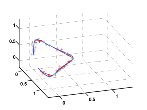
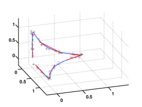
Note that (3) cannot be solved without retaining all previous data in memory, which is impractical for the applications of interest. To address this, we instead consider an approximation to the cost function in (3) of the form $F(\mathcal{M})+\mu\operatorname{pen}(\mathcal{M})$, where $F(\mathcal{M})$ measures how well the data fits $\mathcal{M}$. In Section III, we will show several forms of $F(\mathcal{M})$ that lead to recursive updates and efficient tracking algorithms, and present our new algorithm: Multi-scale Online Union of SubSets Estimate (MOUSSE). Our method finds a sequence of approximations $\widehat{\mathcal{M}}_{1},\ldots,\widehat{\mathcal{M}}_{t}$, such that $\widehat{\mathcal{M}}_{t+1}$ is computed by updating the previous approximation $\widehat{\mathcal{M}}_{t}$ using $F(\mathcal{M})$ and the current datum $x_{t+1}$ (but not older data). One example of a MOUSSE approximation is illustrated in Figure 1. In this figure, the dashed line corresponds to the true submanifold, the red lines correspond to the estimated union of subsets by MOUSSE, and the $+$ signs correspond to the past 500 samples, with darker colors corresponding to more recent observations. The context is described in more detail in Section VI-C.

Given the sequence of submanifold estimates $\widehat{\mathcal{M}}_{1},\ldots,\widehat{\mathcal{M}}_{t}$, we can compute the distance of each $x_{t}$ to $\widehat{\mathcal{M}}_{t}$, which we refer to as residuals and denote using $\{e_{t}\}$. We then apply change-point detection methods to the sequence of tracking residuals $\{e_{t}\}$. In particular, we assume that when there is no change-point, the $e_{t}$ are i.i.d. with distribution $\nu_{0}$. When there is a change-point, there exists an unknown time $\kappa<t$ such that $e_{1},\ldots,e_{\kappa}$ are i.i.d. with distribution $\nu_{0}$, and $e_{\kappa+1},\ldots$ are i.i.d. with distribution $\nu_{1}$. Our goals are to (a) detect as soon as possible when such a $\kappa$ exists before $t$ and (b) when no such $\kappa$ exists, have our method accept streaming data for as long as possible before falsely declaring a change-point. (Note that in this setting, even if no change-point exists and all data are i.i.d., any method will eventually incorrectly declare a change-point; that is, for an infinite stream of data, we will have a false alarm at some time with probability one. However, good change-point detection methods ensure that, with high probability, these false detections only occur after a very long waiting time, and thus exert some measure of control over the false alarm rate over time.)

Figure 1: Approximation of MOUSSE at $t=250$ (upper) and $t=1150$ (lower) of a 100-dimensional submanifold. In this figure we project everything into three-dimensional space. The blue curve corresponds to true submanifold, the plus signs are noisy samples from the submanifold (the lighter plus signs are more dated than the darker plus signs), and the red line segments are the approximation subsets computed with MOUSSE. As the curvature of the submanifold increases, MOUSSE also adapts in the number of subsets.

III Multiscale Online Union of Subsets Estimation (MOUSSE)

In this section, we describe the Multiscale Online Union of SubSets Estimation (MOUSSE) method, including the underlying multiscale model and online update approaches.

III-A Multiscale union of subsets model

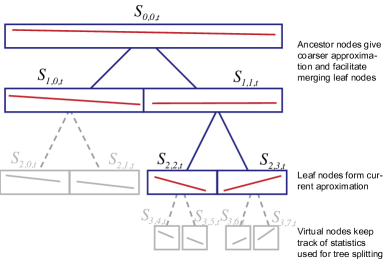
MOUSSE uses a union of low-dimensional subsets, $\widehat{\mathcal{M}}_{t}$, to approximate $\mathcal{M}_{t}$, and organizes these subsets using a tree structure. The idea for a multiscale tree structure is drawn from the multiscale harmonic analysis literature [43]. The leaves of the tree are subsets that are used for the submanifold approximation. Each node in the tree represents a local approximation to the submanifold at one scale. The parent nodes are subsets that contain coarser approximations to the submanifold than their children. The subset associated with a parent node roughly covers the subsets associated with its two children.

More specifically, our approximation at each time $t$ consists of a union of subsets $\mathcal{S}_{j,k,t}$ that is organized using a tree structure. Here $j\in\{1,\ldots,J_{t}\}$ denotes the scale or level of the subset in the tree, where $J_{t}$ is the tree depth at time $t$, and $k\in\{1,\ldots,2^{j}\}$ denotes the index of the subset for that level. The approximation $\widehat{\mathcal{M}}_{t}$ at time $t$ is given by:

$$\widehat{\mathcal{M}}_{t}=\bigcup_{(j,k)\in\mathcal{A}_{t}}\mathcal{S}_{j,k,t},$$ (4)

where $\mathcal{A}_{t}$ contains the indices of all leaf nodes used for approximation at time $t$. Also define $\mathcal{T}_{t}$ to be the set of indices of all nodes in the tree at time $t$, with $\mathcal{A}_{t}\subset\mathcal{T}_{t}.$ Each of these subsets lies on a low-dimensional hyperplane with dimension $d$ and is parameterized as

$$\begin{split}\mathcal{S}_{j,k,t}&=\{v\in\mathbb{R}^{D}:v=U_{j,k,t}z+c_{j,k,t},\\ &\qquad\qquad\quad~{}~{}z^{\top}\Lambda_{j,k,t}^{-1}z\leq 1,\quad z\in\mathbb{R}^{d}\},\end{split}$$ (5)

where the notation ^⊤ denotes transpose of a matrix or vector. The matrix $U_{j,k,t}\in\mathbb{R}^{D\times d}$ is the subspace basis, and $c_{j,k,t}\in\mathbb{R}^{D}$ is the offset of the hyperplane from the origin. The diagonal matrix

$${\Lambda}_{j,k,t}\triangleq\mbox{diag}\{\lambda_{j,k,t}^{(1)},\ldots,\lambda_{j,k,t}^{(d)}\}\in\mathbb{R}^{d\times d},$$

with $\lambda_{j,k,t}^{(1)}\geq\ldots\geq\lambda_{j,k,t}^{(d)}\geq 0$, contains eigenvalues of the covariance matrix of the projected data onto each hyperplane. This parameter specifies the shape of the ellipsoid by capturing the spread of the data within the hyperplane. In summary, the parameters for $\mathcal{S}_{j,k,t}$ are

$$\{U_{j,k,t},c_{j,k,t},\Lambda_{j,k,t}\}_{(j,k)\in\mathcal{T}_{t}},$$

and these parameters will be updated online, as described in Algorithm 2.

In our tree structure, the leaf nodes of the tree also have two virtual children nodes that maintain estimates for corresponding subsets at a finer scale than encapsulated by the leaf nodes of our tree (and $\widehat{\mathcal{M}}_{t}$); these subsets are not used for our instantaneous submanifold approximation, but rather when further subdivision with the tree is needed. We will explain more details about tree subdivision and growth in Section III-E and Algorithms 3 and 4. The complexity of the approximation, denoted $K_{t}$, is defined to be the total number of subsets used for approximation at time $t$:

$$K_{t}\triangleq|\mathcal{A}_{t}|;$$ (6)

this is used as the complexity regularization term in (3): $\operatorname{pen}(\widehat{\mathcal{M}}_{t})\triangleq K_{t}.$ The tree structure is illustrated in Figure 2.

Figure 2: Illustration of tree structure for subsets. The subsets used in our approximation are $\{\mathcal{S}_{1,0,t}\cup\mathcal{S}_{2,2,t}\cup\mathcal{S}_{2,3,t}\}$.

III-B Approximate Mahalanobis distance

To update the submanifold approximation, we first determine the affinity of $x_{t+1}$ to each subset. We might simply project $x_{t+1}$ onto each subset (i.e. ellipsoid), but computing this projection generally requires using numerical solver. Alternatively, we could consider the Mahalanobis distance, which is commonly used for data classification and it measures the quadratic distance of $x$ to a set $\mathcal{S}$ of data with mean $c=\mathbb{E}\{x\}$ and covariance $\Sigma=\mathbb{E}\{(x-c)(x-c)^{\top}\}$. Specifically, the Mahalanobis distance is defined as

$$\varrho(x,\mathcal{S})=(x-c)^{\top}\Sigma^{-1}(x-c).$$ (7)

However, this distance is only finite and well-defined for points lying in one of the low dimensional subspaces in our approximation. Since our construction is a piecewise linear approximation to a submanifold which may have some curvature, we anticipate many observations which are near but not in our collection of subsets, and we need a well-defined, finite distance measure for such points.

To address these challenges, we introduce the approximate Mahalanobis distance of a point $x$ to a subset $\mathcal{S}$, which is a hybrid of Euclidean distance and Mahalanobis distance. Assume $x$ with support $\Omega$ and the parameters for a set $\mathcal{S}$ is given by $\{U,c,\Lambda\}$. Define

$$U_{\Omega}\triangleq\mathcal{P}_{\Omega}U\in\mathbb{R}^{|\Omega|\times d},\quad c_{\Omega}\triangleq\mathcal{P}_{\Omega}c\in\mathbb{R}^{|\Omega|},$$

and

$$x_{\Omega}=\mathcal{P}_{\Omega}x\in\mathbb{R}^{|\Omega|}.$$

Define the pseudoinverse operator that computes the coefficients of a vector in the subspace spanned by $V$ as

$$V^{\#}\triangleq(V^{\top}V)^{-1}V^{\top}.$$ (8)

Let $U^{\top}_{\Omega}$ denote $(U_{\Omega})^{\top},$ and similarly $U^{\#}_{\Omega}=(U_{\Omega})^{\#}$. When $U$ is an orthogonal matrix, we have $U^{\#}\equiv U^{\top}$, but in general $U_{\Omega}^{\#}\neq U_{\Omega}^{\top}$. Let

$$\beta=U_{\Omega}^{\#}(x_{\Omega}-c_{\Omega}),$$ (9)

and

$$x_{\perp}=(I-U_{\Omega}U_{\Omega}^{\#})(x_{\Omega}-c_{\Omega}).$$ (10)

In this definition, $\beta$ is the projection coefficient of a re-centered $x$ on ${\color[rgb]{0,0,0}{U_{\Omega}}}$, and $x_{\perp}$ captures the projection residual. Assuming the covariance matrix has a low-rank structure with $d$ large eigenvalues and $D-d$ small eigenvalues, we can write the eigendecomposition of the covariance matrix $\Sigma$ as

$$\Sigma\triangleq\begin{bmatrix}U&U_{\perp}\end{bmatrix}\Lambda\begin{bmatrix}U&U_{\perp}\end{bmatrix}^{\top}=U\Lambda_{1}U^{\top}+U_{\perp}\Lambda_{2}U_{\perp}^{\top},$$

where $\Lambda=\mbox{diag}\{\lambda_{1},\ldots,\lambda_{D}\}$, $\lambda_{1}\geq\ldots\geq\lambda_{D}$, $\Lambda_{1}=\mbox{diag}\{\lambda_{1},\ldots,\lambda_{d}\}$, $\Lambda_{2}=\mbox{diag}\{\lambda_{d+1},\ldots,\lambda_{D}\}$. If we further assume that the $D-d$ small eigenvalues are all approximately equal to some $\delta>0$, i.e., $\Lambda_{2}\approx\delta I$, then the Mahalanobis distance (7) may be approximated as

$$\varrho(x,\mathcal{S})\approx(x-c)^{\top}U\Lambda_{1}^{-1}U^{\top}(x-c)+\delta^{-1}\|U_{\perp}^{\top}(x-c)\|^{2}.$$ (11)

Motivated by this, we define the approximate Mahalanobis distance:

$$\rho_{\delta}(x,\mathcal{S})\triangleq{\beta}^{\top}{\Lambda}^{-1}{\beta}+\delta^{-1}\|{x}_{\perp}\|^{2}.$$ (12)

When the data is complete, $\rho_{\delta}(x,\mathcal{S})$ is equal to the right-hand-side of (11), since

$$\beta= (U^{\top}U)^{-1}U^{\top}(x-c)=U^{\top}(x-c),$$

$$x_{\perp}= (I-UU^{\top})(x-c),$$

then we can write the right-hand-side of (11) as $\beta^{\top}\Lambda^{-1}\beta+\delta^{-1}\|x_{\perp}\|^{2}$. With missing data, $\rho_{\delta}(x,\mathcal{S})$ is an approximation to $\varrho(x,\mathcal{S})$.

In definition of the approximation Mahalanobis distance (12), $\delta$ is a small number and has to be estimated from noisy data. To avoid the numerical instability caused when dividing by a small number, we use the following scaled approximate Mahalanobis distance as a measure of the distance between $x$ and a subset:

$$d_{\delta}(x,\mathcal{S})=\delta\rho_{\delta}(x,S)=\delta\beta^{\top}\Lambda^{-1}\beta+\|x_{\perp}\|^{2}.$$ (13)

With this definition, we can find the subset within our approximation with minimum distance to the new datum $x_{t}$:

$$(j^{*},k^{*})=\arg\min_{(j,k)}d_{\delta_{j,k,t}}(x_{t},\mathcal{S}_{j,k,t}).$$ (14)

We can further define the tracking residual of the submanifold at time $t$.

$$\begin{split}e_{t}&\triangleq\left(d_{\delta_{j^{*},k^{*},t}}(x_{t},\mathcal{S}_{j^{*},k^{*},t})\right)^{1/2}\\ &=\left(\delta_{j^{*},k^{*},t}{\beta^{*}}^{\top}{\Lambda}_{j^{*},k^{*},t}^{-1}\beta^{*}+\|{x}_{\perp}^{*}\|^{2}\right)^{1/2},\end{split}$$ (15)

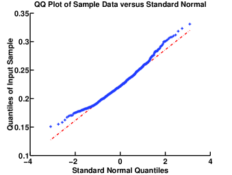
where $\beta^{*}$ and $x_{\perp}^{*}$ are calculated for $x_{t+1}$ relative to $\mathcal{S}_{j^{*},k^{*},t}$ using (9) and (10). We take the square root of the scaled approximate Mahalanobis distance to ensure that the $e_{t}$s can be well modeled as draws from a Gaussian distribution (as demonstrated in Section IV-C).

III-C MOUSSE Algorithm

When a new sample $x_{t+1}$ becomes available, MOUSSE updates $\widehat{\mathcal{M}}_{t}$ to obtain $\widehat{\mathcal{M}}_{t+1}$. The update steps are presented in Algorithm 1; there are three main steps, detailed in the below subsections: (a) find the subset in $\widehat{\mathcal{M}}_{t}$ which is closest to $x_{t+1}$, (b) update a tracking estimate of that closest subset, its ancestors, and its nearest virtual child, and (c) grow or prune the tree structure to preserve a balance between fit to data and complexity. The parameters $\{U_{j,k,t},\Lambda_{j,k,t},c_{j,k,t},\delta_{j,k,t}\}$ are calculated and updated in Algorithm 2. We use $[z]_{m}$ to denote the $m$-th element of a vector $z$.

Algorithm 1 MOUSSE

1:  Input: error tolerance $\epsilon$, step size $\alpha$, relative weight $\mu$

2:  Initialize tree structure, set $\epsilon_{0}=0$

3:  for $t=0,1,\ldots$ do

4:     Given new data $x_{t+1}$ and its support $\Omega_{t+1}$

5:     find the minimum distance set $\mathcal{S}_{j^{*},k^{*},t}$ according to (14)

6:     let $\beta^{*}$ and $x_{\perp}^{*}$ denote (9) and (10) of $x_{t+1}$ for $\mathcal{S}_{j^{*},k^{*},t}$

7:     calculate: $e_{t+1}$ using (15)

8:     update all ancestor nodes and closest virtual child node of $(j^{*},k^{*})$ using Algorithm 2

9:     calculate: $\epsilon_{t+1}=\alpha\epsilon_{t}+e_{t+1}^{2}$

10:     denote parent node of $(j^{*},k^{*})$ as $(j^{*}-1,k_{p})$ and closest virtual child node as $(j^{*}+1,k_{v})$

11:     if $\epsilon_{t+1}>\epsilon$ and $d_{\delta_{j^{*}+1,k_{v},t}}(x_{t+1},\mathcal{S}_{j^{*}+1,k_{v},t})+\mu(K_{t}+1)<d_{\delta_{j^{*},k^{*},t}}(x_{t+1},\mathcal{S}_{j^{*},k^{*},t})+\mu K_{t}$  then

12:        split $(j^{*},k^{*})$ using Algorithm 3

13:     end if

14:     if $\epsilon_{t+1}<\epsilon$ and $d_{\delta_{j^{*}-1,k_{p},t}}(x_{t+1},\mathcal{S}_{j^{*}-1,k_{p},t})+\mu(K_{t}-1)<d_{\delta_{j^{*},k^{*},t}}(x_{t+1},\mathcal{S}_{j^{*},k^{*},t})+\mu K_{t}$  then

15:        merge $(j^{*},k^{*})$ and its sibling using Algorithm 4

16:     end if

17:     update $\mathcal{A}_{t}$ and $\mathcal{T}_{t}$

18:  end for

Algorithm 2 Update node

1:  Input: node index $(j,k)$, $\alpha$, $\delta$ and subspace parameters

2:  Calculate: ${\beta}$ and $x_{\perp}$ using (9) and (10)

3:  Update: $[c_{j,k,t+1}]_{m}=\alpha[c_{j,k,t}]_{m}+(1-\alpha)[x_{t+1}]_{m}$, $m\in\Omega_{t+1}$

4:  Update: $\lambda_{j,k,t+1}^{(m)}=\alpha\lambda_{j,k,t}^{(m)}+(1-\alpha)[\beta]_{m}^{2},m=1,\ldots,d$

5:  Update: $\delta_{j,k,t+1}=\alpha\delta_{j,k,t}+(1-\alpha)\|x_{\perp}\|^{2}/(D-d)$

6:  Update basis $U_{j,k,t}$ using (modified) subspace tracking algorithm

Algorithm 3 Split node $(j,k)$

1:  Turn two virtual children nodes $(j+1,2k)$ and $(j+1,2k+1)$ of node $(j,k)$ into leaf nodes

2:  Initialize virtual nodes $(j+1,2k)$ and $(j+1,2k+1)$:

$$k_{1} =2k$$

$$k_{2} =2k+1$$

$$c_{j+1,k_{1},t+1} =c_{j,k,t}+\sqrt{\lambda_{j,k,t}^{(1)}}u^{(1)}_{j,k,t}/2$$

$$c_{j+1,k_{2},t+1} =c_{j,k,t}-\sqrt{\lambda_{j,k,t}^{(1)}}u^{(1)}_{j,k,t}/2$$

$$U_{j+1,k_{i},t+1} =U_{j,k,t},\quad i=1,2$$

$$\lambda_{j+1,k_{i},t+1}^{(1)} =\lambda_{j,k,t}^{(1)}/2,\quad i=1,2$$

$$\lambda_{j+1,k_{i},t+1}^{(m)} =\lambda_{j,k,t}^{(m)},\quad m=2,\ldots,d,\quad i=1,2$$

Algorithm 4 Merge $(j,k)$ and its sibling

1:  Make the parent node of $(j,k)$ into a leaf node

2:  Make $(j,k)$ and its sibling into virtual children nodes of the newly created leaf

3:  Delete all four virtual children nodes of $(j,k)$ and its sibling

III-D Update subset parameters

When updating subsets, we can update all subsets in our multiscale representation and make the update step-size to be inversely proportional to the approximate Mahalanobis distance between the new sample and each subset, which we refer to as the “update-all” approach. Alternatively, we can just update the subset closest to $x_{t+1}$, its virtual children, and all its ancestor nodes, which we refer to as the “update-nearest” approach. The update-all approach is computationally more expensive, especially for high dimensional problems, so we focus our attention on the greedy update-nearest approach. The below approaches extend readily to the update-all setting, however.

In the update-nearest approach, we update the parameters of the minimum distance subset defined in (14), all its ancestors in the tree, and its two virtual children. The update algorithm is summarized in Algorithm 2 which denotes the parameters associated with $\mathcal{S}_{j^{*},k^{*},t}$ as $(c,U,\Lambda,\delta)$, and drops the $j^{*}$, $k^{*}$, and $t$ indices for simplicity of presentation. The update of the center $c$, $\Lambda$ and $\delta$ are provided in the following, Sections A and B.

To decide whether to change the tree structure, we introduce the average residual for a “forgetting factor” $\alpha\in(0,1)$:

$$\begin{split}\epsilon_{t}&\triangleq\sum_{i=1}^{t}\alpha^{t-i}e_{i}^{2}\\ &={\color[rgb]{0,0,0}{\alpha\epsilon_{t-1}+e_{t}^{2}.}}\end{split}$$ (16)

We will consider changing the tree structure when $\epsilon_{t}$ is greater than our prescribed residual tolerance $\epsilon>0$.

Next we will focus on three approaches to updating $U$ by modifying existing subspace tracking methods. In the following, for tractability reasons, we hold $\Lambda$ fixed and update with respect to $U$ alone at first. We then update the shape parameters $\Lambda$ and $\delta$ for fixed $U$.

III-D1 GROUSE

To use GROUSE subspace tracking in this context, we approximate the first term in (3) as

$$\begin{split}F(\mathcal{M})=&\sum_{i=1}^{t}\alpha^{t+1-i}\|\mathcal{P}_{\Omega_{i}}(x_{i}-\mathcal{P}_{\widehat{\mathcal{M}}_{i}}x_{i})\|^{2}\\ &+\|\mathcal{P}_{\Omega_{t+1}}(x_{t+1}-\mathcal{P}_{\mathcal{M}}x_{t+1})\|^{2}.\end{split}$$ (17)

Note the first term is a constant with respect to $\mathcal{M}$, so we need only to consider the second term in computing an update. To focus on updating subspace without the shape parameters, we replace $\|\mathcal{P}_{\Omega_{t+1}}(x_{t+1}-\mathcal{P}_{\mathcal{M}}x_{t+1})\|^{2}$ in (17) by

$$f(U)\triangleq\min_{a}\|\mathcal{P}_{\Omega_{t+1}}(x_{t+1}-Ua-c)\|^{2}$$ (18)

(assuming $U$ is orthonormal and including the offset vector $c$). The basic idea is now to take a step in the direction of the instantaneous gradient of this cost function (18). This task corresponds to the basis update of GROUSE [17] with the cost function (18).

Following the same derivation as in [17], we have that

$$\frac{df}{dU}=-2\mathcal{P}_{\Omega_{t+1}}(x_{t+1}-c-U\beta)\beta^{\top}\triangleq-2r\beta^{\top},$$ (19)

where $\beta$ is defined in (9), and

$$r=\mathcal{P}_{\Omega_{t+1}}(x_{t+1}-c-U\beta).$$

The gradient on the Grassmannian is given by

$$\nabla f=(I-UU^{\top})\frac{df}{dU}=-2(I-UU^{\top})r\beta^{\top}=-2r\beta^{\top},$$

since $U^{\top}r=0$. We obtain that the update of $U_{t}$ using the Grassmannian gradient is given by

$$U_{t+1}=U_{t}+\frac{\cos(\xi\eta)-1}{\|\beta\|^{2}}U_{t}\beta\beta^{\top}+\sin(\xi\eta)\frac{r}{\|r\|}\frac{\beta^{\top}}{\|\beta\|},$$

where $\eta>0$ is the step-size, and $\xi=\|r\|\|U_{t}\beta\|$. The step-size $\eta$ is chosen to be $\eta=\eta_{0}/\|x_{t+1}\|$, for a constant $\eta_{0}>0$.

III-D2 PETRELS

Let $(j^{*},k^{*})$ denote the indices of the closest subset to $x_{t+1}$, and let $\mathcal{I}_{t}\subseteq\{1,\ldots,t,t+1\}$ denote the set of times corresponding to data which were closest to this subset and used to estimate its parameters in previous rounds. Then we can write

$$\begin{split}F(\mathcal{M})=&\sum_{i\notin\mathcal{I}_{t}}\alpha^{t-i}\|\mathcal{P}_{\Omega_{i}}(x_{i}-\mathcal{P}_{\widehat{\mathcal{M}}_{i}}x_{i})\|^{2}\\ &+\sum_{i\in\mathcal{I}_{t}}\alpha^{t-i}\|\mathcal{P}_{\Omega_{i}}(x_{i}-\mathcal{P}_{\mathcal{M}}x_{i})\|^{2}.\end{split}$$ (20)

where, as before, the first sum is independent of $\mathcal{M}$ and can be ignored during minimization. When focusing on updating $U$ for fixed $\Lambda$, the minimization of $F(\mathcal{M})$ with respect to the subspace $U$ used for node $(j^{*},k^{*})$ in (20) can be accomplished using the PETRELS algorithm [44], yielding a solution which can be expressed recursively as follows. Denoting by $[U]_{m}$ the $m$-th row of $U$, we have the update of $U$ given by

$$\begin{split}&[U_{t+1}]_{m}=[U_{t}]_{m}\\ &+I_{m\in\Omega_{t}}([U_{t}a_{t+1}]_{m}-a_{t+1}^{\top}[U_{t}]_{m})(R_{m,t+1})^{\#}a_{t+1},\end{split}$$ (21)

for $m=1,\ldots,D$, where $I_{A}$ is the indicator function for event $A$, and

$$a_{t+1}=(U_{t}^{\top}\mathcal{P}_{\Omega_{t+1}}U_{t})^{\#}U_{t}^{\top}x_{t+1}.$$

The second-order information in $R_{m,t+1}$ can be computed recursively as

$$\begin{split}&(R_{m,t+1})^{\#}=\alpha^{-1}(R_{m,t})^{\#}\\ &+\frac{\alpha^{-2}p_{m,t+1}}{1+\alpha^{-1}a_{t+1}^{\top}(R_{m,t})^{\#}a_{t+1}}(R_{m,t})^{\#}a_{t}a_{t}^{\top}(R_{m,t})^{\#}.\end{split}$$ (22)

Note that PETRELS does not guarantee the orthogonality of $U_{t+1}$, which is important for quickly computing projections onto our submanifold approximation. To obtain orthonormal $U_{t+1}$, we may apply Gram-Schmidt orthonormalization after each update. We refer to this modification of PETRELS as PETRELS-GS. This orthogonalization requires an extra computational cost on the order of $\mathcal{O}(Dd^{2})$ and may compromise the continuity of $U_{t}$, i.e., the Frobenius norm $\|U_{t+1}-U_{t}\|_{F}$ after the orthogonalization may not be small even when the corresponding subsets are very close [45]. This lack of continuity makes it impossible to effectively track the scale parameter $\Lambda$. A faster orthonormalization (FO) strategy with less computation which also preserves the continuity of $U_{t}$ is given in [45]. We refer to this FO strategy combined with PETRELS as PETRELS-FO.

III-D3 Computational complexity

For each update with complete data (which is more complex than an update with missing data), the computational complexity of GROUSE is on the order of $\mathcal{O}(Dd)$, PETRELS-GS is $\mathcal{O}(Dd^{2})$, and PETRELS-FO is $\mathcal{O}(Dd)$. More details about the relative performance of these three subspace update methods can be found in Section VI.

III-E Tree structure update

When the curvature of the submanifold changes and cannot be sufficiently characterized by the current subset approximations, we must perform adaptive model selection. This can be accomplished within our framework by updating the tree structure – growing the tree or pruning the tree, which we refer to as “splitting” and “merging” branches, respectively. Previous work has derived finite sample bounds and convergence rates of adaptive model selection in nonparametric time series prediction [46].

Splitting tree branches increases the resolution of the approximation at the cost of higher estimator complexity. Merging reduces resolution but lowers complexity. When making decisions on splitting or merging, we take into consideration the approximation residuals as well as the model complexity (the number of subsets $K_{t}$ used in the approximation). This is related to complexity-regularized tree estimation methods [47, 43, 48] and the notion of minimum description length (MDL) in compression theory [49, 50]. In particular, we use the sum of the average residuals and a penalty proportional to the number of subsets used for approximation as the cost function when deciding to split or merge. The splitting and merging operations are detailed in Algorithm 3 and Algorithm 4. The splitting process mimics the $k$-means algorithm. In these algorithms, note that for node $(j,k)$ the parent is node $(j-1,\lfloor k/2\rfloor)$ and the sibling node is $(j,k+1)$ for $k$ even or $(j,k-1)$ for $k$ odd.

III-F Initialization

To initialize MOUSSE, we assume a small initial training set of samples, and perform a nested bi-partition of the training data set to form a tree structure, as shown in Figure 2. The root of the tree represents the entire data set, and the children of each node represent a bipartition of the data in the parent node. The bipartition of the data can be performed by the $k$-means algorithm. We start with the entire data, estimate the sample covariance matrix, perform an eigendecomposition, extract the $d$-largest eigenvectors and eigenvalues and use them for $U_{1,1,0}$ and $\Lambda_{1,1,0}$, respectively. The average of the $(D-d)$ minor eigenvalues are used for $\delta_{1,1,0}$. If the approximation residual is greater than the prescribed residual tolerance $\epsilon$, we further partition the data into two clusters using $k$-means (for $k=2$) and repeat the above process. We keep partitioning the data until $\delta_{j,k,0}$ is less than $\epsilon$ for all leaf nodes. Then we further partition the data one level down to form the virtual children nodes. This tree construction is similar to that used in [15].

In principle, it is possible to bypass this training phase and just initialize the tree with a single root node and two random virtual children nodes. However, the training phase makes it much easier to select algorithm parameters such as $\epsilon$ and provides more meaningful initial virtual nodes, thereby shortening the “burn in” time of the algorithm.

III-G Choice of parameters

In general, $\alpha$ should be close to 1, as in the Recursive Least Squares (RLS) algorithm [51]. In the case when the submanifold changes quickly, we would expect smaller weights for approximation based on historical data and thus a smaller $\alpha$. In contrast, a slowly evolving submanifold requires a larger $\alpha$. In our experiments, $\alpha$ ranges from 0.8 to 0.95. $\epsilon$ controls residual tolerance, which varies from problem to problem according to the smoothness of the submanifold underlying the data and the noise variance. Since the tree’s complexity is controlled and $\operatorname{pen}({\mathcal{M}})$ in (3) is roughly on the order of $\mathcal{O}(1)$, we usually set $\mu$ close to $\epsilon$.

IV Change-point detection

We are interested in detecting changes to the submanifold that arise abruptly and change the statistics of the data. When the submanifold varies slowly in time, MOUSSE (described in Section III) can track the submanifold and produce a sequence of stationary tracking residuals. Because MOUSSE uses a bounded small step-size, and only allows merging or splitting by one level in the tree structure update, when an abrupt change occurs, MOUSSE will lose track of the manifold, resulting in an abrupt increase in the magnitude of the tracking residuals. This abrupt change in tracking residuals enables change-point detection. In this section, we formulate the change-point problem using MOUSSE residuals $e_{t}$, show that the distribution of $e_{t}$ is close to Gaussian, and adapt the generalized-likelihood ratio (GLR) procedure [42] for change-point detection.

IV-A Generalized likelihood ratio (GLR) procedure

We adopt the quickest change-point detection formulation to detect an abrupt change in the distribution of the residuals. In particular, we assume that $\nu_{0}$ is a normal distribution with mean $\mu_{0}$ and variance $\sigma_{0}^{2}$, and $\nu_{1}$ is a normal distribution with mean $\mu_{1}$ and the same variance $\sigma_{0}^{2}$. Then we can formulate the change-point detection problem as the following hypothesis test:

$$\begin{split}\textsf{H}_{0}:&\quad e_{1},\ldots,e_{t}\sim\mathcal{N}(\mu_{0},\sigma_{0}^{2}),\\ \textsf{H}_{1}:&\quad e_{1},\ldots,e_{\kappa}\sim\mathcal{N}({\color[rgb]{0,0,0}{\mu_{0}}},\sigma_{0}^{2}),\quad e_{\kappa+1},\ldots,e_{t}\sim\mathcal{N}(\mu_{1},\sigma_{0}^{2}).\end{split}$$ (23)

In the case where the pre-change and post-change distributions are completely specified, two very good procedures are the CUSUM test [52, 53] and the quasi-Bayesian Shiryayev-Roberts procedure [54, 55] (also see [2, 56] for surveys). The CUSUM and Shiryayev-Roberts procedures minimize asymptotically to first order the maximum expected delay in detecting a change-point, under different conditions (see [53] for CUSUM and [57, 58] for Shiryayev-Roberts procedures).

In our problem, the post-change distribution is not completely prescribed. We assume $\mu_{0}$ and $\sigma_{0}^{2}$ are known since typically there is enough normal data to estimate these parameters (when the training phase is too short for this to be the case, these quantities can be estimated online, as described in [59]). However, we assume $\mu_{1}$ is unknown since the magnitude of the change-point can vary from one instance to another. With this assumption, we instead use the generalized likelihood ratio (GLR) procedure [42] (which is derived based on the CUSUM procedure), by replacing $\mu_{1}$ with its maximum likelihood estimate (for each fixed change-point time $\kappa=k$):

$$\hat{\mu}_{1}=\frac{S_{t}-S_{k}}{t-k},$$

where

$$S_{t}\triangleq\sum_{i=1}^{t}e_{i}.$$

We compute a GLR statistic at each time $t$ and stop (declare a detected change-point) the first time the statistic hits a threshold $b$:

$$T=\inf\Big{\{} t\geq 1:\max_{t-w\leq k<t}\frac{|(S_{t}-S_{k})-\mu_{0}(t-k)|}{\sigma_{0}\sqrt{t-k}}\geq b\Big{\}},$$ (24)

where $w$ is a time-window length such that we only consider the most recent $w$ residuals for change-point detection, and the threshold $b$ is chosen to control the false-alarm-rate, which is characterized using average-run-length (ARL) in the change-point detection literature [60]. Typically we would choose $w$ to be several times (for example, 5 to 10 times) of the anticipated detection delay, then the window length will almost have no effect on the detection delay [61]. This threshold choice is detailed in Section IV-B.

IV-B Choice of threshold for change-point detection

In accordance with standard change-point detection notation, denote by $\mathbb{E}^{\infty}$ the expectation when there is no change, i.e., $\mathbb{E}_{\textsf{H}_{0}}$, and by $\mathbb{E}^{k}$ the expectation when there is a change-point at $\kappa=k$, i.e., $\mathbb{E}_{\textsf{H}_{1},\kappa=k}$. The performance metric for a change-point detection algorithm is typically characterized by the expected detection delay $\sup_{k\geq 0}\mathbb{E}^{k}\{T-k|T>k\}$ and the average-run-length (ARL) $\mathbb{E}^{\infty}\{T\}$ [60]. Typically we use $\mathbb{E}^{0}\{T\}$ as a performance metric since it is an upper bound for $\sup_{k\geq 0}\mathbb{E}^{k}\{T-k|T>k\}$. Note that the GLR procedure (24) is equivalent to

$$T=\inf\{t\geq 1:\max_{t-w\leq k<t}\frac{|\tilde{S}_{t}-\tilde{S}_{k}|}{\sqrt{t-k}}\geq b,\}$$ (25)

where $\tilde{S}_{t}=\sum_{i=1}^{t}(e_{i}-\mu_{0})/\sigma_{0}$. Under $H_{0}$, we have $(e_{i}-\mu_{0})/\sigma_{0}$ i.i.d. Gaussian distributed with zero mean and unit variance. Using the results in [42], we have the following approximation. When $b\rightarrow\infty$,

$$\mathbb{E}^{\infty}\{T\}\sim\frac{(2\pi)^{1/2}\exp\{b^{2}/2\}}{b\int_{0}^{b}x\nu^{2}(x)dx},$$ (26)

where $\nu(x)=\frac{(2/x)[\Phi(x/2)-0.5]}{(x/2)\Phi(x/2)+\phi(x)/2}$ [61], $\phi(x)$ and $\Phi(x)$ are the pdf and cdf of the normal random variable with zero mean and unit variance. We will demonstrate in Section VI-E that this asymptotic approximation is fairly accurate even for finite $b$ and when $e_{t}$’s are not exactly Gaussian distributed, which allows us to choose the change-point detection threshold to achieve a target ARL without parameter tuning.

IV-C Distribution of $e_{t}$

In deriving the GLR statistics we have assumed that $e_{t}$ are i.i.d. Gaussian distributed. A fair question to ask is whether $e_{t}$ is truly Gaussian distributed, or even to ask whether $e_{t}$ is a good statistic to use. We can verify that Gaussian distribution is a good approximation for the distribution of $e_{t}$ (15). The QQ-plot of $e_{t}$ from one of our numerical examples in Section  VI when $D=100$ is shown in Figure 3. We will also demonstrate in Section VI-E that the theoretical approximation for ARL using a Gaussian assumption on $e_{t}$ is quite accurate.

Figure 3: Q-Q plot of $e_{t}$, for a $D=100$ submanifold.

V Performance Analysis

In this section, we first study the performance of MOUSSE, and then study the choice for the threshold parameter of the change-point detection algorithm and provide theoretical approximations. A complete proof of convergence of MOUSSE (or GROUSE or PETRELS) is challenging since the space of submanifold approximations we consider is non-convex. Nevertheless, we can still characterize several aspects of our approach.

V-A MOUSSE residuals

As mentioned earlier, our multiscale subset model is closely related to geometric multiresolution analysis (GMRA) [15]. In that work, the authors characterize the favorable approximation capabilities of the proposed multiscale model. In particular, they prove that the magnitudes of the geometric wavelet coefficients associated with their algorithm decay asymptotically as a function of scale, so a collection of data lying on a smooth submanifold can be well-approximated with a small number (depending on the submanifold curvature) of relatively large geometric wavelets. These geometric wavelets are akin to the leaf nodes in our approximation, so the approximation results of [15] suggest that our model admits accurate approximations of data on smooth submanifolds with a small number of leafs.

V-B Optimality and consistency

In Appendix A, we show that the estimate of $c$ is optimal in the complete data setting. In Appendix B, we show that the estimates of $\Lambda$ and $\delta$ are consistent in the complete data setting.

V-C Missing data

In this section, we show that $\beta$ and $x_{\perp}$, when using a missing data projection, are close to their counterparts when using a complete data projection. Hence, when the fraction of missing data is not large, the performance of MOUSSE with missing data is also consistent. In this section, we omit the subscripts $j$, $k$ and $t$, and denote $\Omega_{t}$ by $\Omega$ to simplify notation. Define the coherence of the basis $U$ as [62]

$$\textsf{coh}(U)=\frac{D}{d}\max_{m}\|UU^{\#}\textsf{e}_{m}\|_{2}^{2}.$$ (27)

Theorem 1

Let $\varepsilon>0$. Given $x=v+w$, and $w$ is a white Gaussian noise with zero mean and covariance matrix $\sigma^{2}I_{D\times D}$. Let $\beta=U^{\top}(x-c)$, and $\beta_{\Omega}=U_{\Omega}^{\#}(x_{\Omega}-c_{\Omega})$. If for some constant $\ell\in(0,1)$,

$$|\Omega|\geq\max\left\{\frac{8}{3}\textsf{coh}(U)d\log(2d/\varepsilon),\frac{4}{3}\frac{D}{(1-\ell)\log(2D/\varepsilon)}\right\},$$ (28)

then with probability at least $1-3\varepsilon$,

$$\begin{split}\|\beta_{\Omega}-\beta\|_{2}^{2}\leq&2\frac{(1+\theta)^{2}}{(1-\ell)^{2}}\cdot\frac{d}{|\Omega|}\cdot\textsf{coh}(U)\|q\|^{2}+\sigma^{2}\frac{(64/9)D^{2}}{(1-\ell)^{2}|\Omega|^{2}},\end{split}$$ (29)

where

$$\theta=\sqrt{2\frac{D\max_{n=1}^{D}|[q]_{n}|^{2}}{\|q\|^{2}}\log(1/\varepsilon)},$$

and $q\triangleq(I-UU^{\top})(v-c)$.

The proof of Theorem 1 combines techniques from [62] with a new noise bound. Different from [62], instead of bounding $\|v_{\Omega}-U_{\Omega}\beta_{\Omega}\|$ using $\|v-U\beta\|$, we need to bound $\|\beta-\beta_{\Omega}\|$ using $\|v-U\beta\|$. The proof of this theorem can be found in Appendix C. The first term in the lower-bound (28) is a consequence of Lemma 3 in [62]. This theorem shows that the number of non-zero entries, $|\Omega|$, should be on the order of the maximum of $d\log d$ and $D/\log(D)$ for accurate estimation of $\beta_{\Omega}$. The first term in the bound (29) is proportional to $\|q\|$, which is related to the distance of $v$ from $U$, and the second term in (29) is due to noise.

VI Numerical Examples

In this section, we present several numerical examples, first based on simulated data, and then real data, to demonstrate the performance of MOUSSE in tracking a submanifold and detecting change-points. We also verify that the theoretical approximation to ARL in Section IV-B is quite accurate.

VI-A Comparison of tracking algorithms

We first compare the performance of different tracking algorithms presented in Section III-D: GROUSE, PETRELS-GS and PETRELS-FO in tracking a time varying manifold. The dimension of the submanifold is $D=100$ and the intrinsic dimension is $d=1$. Fixing $\theta\in[-2,2]$, we define $v(\theta)\in\mathbb{R}^{D}$ with its $n$-th element

$$[v(\theta)]_{n}=1/\sqrt{2\pi}e^{-(z_{n}-\theta)^{2}/(2\gamma_{t}^{2})},$$ (30)

where $z_{n}=-2+4n/D$, $n=1,\ldots,100$, corresponds to regularly spaced points between $-2$ and $2$. Let $\gamma_{t}$ be time-varying:

$$\gamma_{t}=\left\{\begin{array}[]{ll}0.6-\gamma_{0}t,&t=1,2,\dots,s,\\ 0.6-\gamma_{0}(2s-t),&t=s+1,s+2,\dots,2s,\end{array}\right.$$ (33)

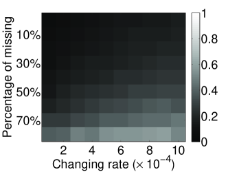
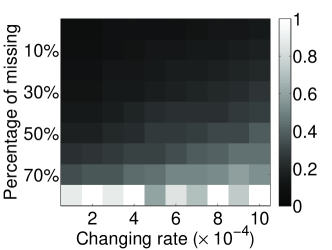
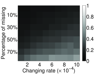
where parameter $\gamma_{0}$ controls how fast the submanifold changes, and $s=1000$. The observation $x_{t}$ is obtained from (1) with noise variance $\sigma^{2}=4\times 10^{-4}$. We compare the methods with various settings of changing rate $\gamma_{0}$ and percentage of missing entries in $x_{t}$.

In the following experiments, we use sample average approximation error $\varepsilon_{N}$ obtained from $N=1200$ samples $\{y_{1},\ldots,y_{N}\}$ as a metric for comparison:

$$\mathbb{E}\{e_{t}^{2}\}\approx\frac{1}{N}\sum_{i=1}^{N}e_{i}^{2},$$ (34)

where $\mathcal{S}_{i}$ denotes the minimum distance subset for sample $y_{i}$. We set the parameters for each tracking algorithm such that they each having the best numerical performance. We use $d=1$ for MOUSSE in all instances. The comparison results are displayed in Figure 4, where the horizontal axis is the submanifold changing rate $\gamma_{0}$, the vertical axis is the percentage of missing data, and the brightness of each block corresponds to our numerical estimate of $\mathbb{E}\{e_{t}^{2}\}$. In Figure 4, PETRELS-FO performs far better then PETRELS-GS and slightly better than GROUSE, especially with a large fraction of missing data. For PETRELS-FO, the best parameters are fairly stable for various combinations of submanifold changing rates and factions of missing data: with $\alpha$ around 0.9, $\mu$ around 0.2, and $\epsilon$ around 0.1. Considering its lower computational cost and ease of parameter tuning, we adopt PETRELS-FO in MOUSSE for the remaining experiments in this paper.

(a) $\mathbb{E}\{e_{t}^{2}\}$ of MOUSSE using GROUSE

(b) $\mathbb{E}\{e_{t}^{2}\}$ of MOUSSE using PETRELS-GS

(c) $\mathbb{E}\{e_{t}^{2}\}$ of MOUSSE using PETRELS-FO

Figure 4: MOUSSE tracking a slowly varying submanifold using: (a) GROUSE, (b) PETRELS-GS and (c) PETRELS-FO. Horizontal axis corresponds to rate of change for submanifold and vertical axis corresponds to fraction of data missing. Brightness corresponds to $\mathbb{E}\{e_{t}^{2}\}$.

VI-B Tracking a static submanifold

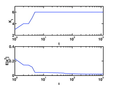
We then study the performance of MOUSSE tracking a static submanifold. The dimension of the submanifold is $D=100$ and the intrinsic dimension is $d=1$. Fixing $\theta\in[-2,2]$, we define $v(\theta)\in\mathbb{R}^{D}$ according to (30) with $\gamma_{t}=\gamma=0.6$ for all $t$. The observation $x_{t}$ is obtained from (1) with noise variance $\sigma^{2}=4\times 10^{-4}$. We set $d=1$ (the assumed intrinsic dimension is identical to the true $d$), $\alpha=0.95$, $\epsilon=0.1$, $\mu=0.1$, and use PETRELS-FO for subspace tracking. Figure 5 demonstrates that MOUSSE is able to track a static submanifold and reach the steady state quickly from a coarse initialization.

Figure 5: MOUSSE tracking a static submanifold with $D=100$ and $d=1$.

VI-C Tracking a slowly time-varying submanifold

Next we looking closely at MOUSSE tracking a slowly time-varying submanifold. Consider the submanifold defined in (33), with $D=100$ and $d=1$. We set the assumed intrinsic dimension to be identical to the true $d$, choose $\gamma_{0}=2\times 10^{-4}$, $s=1000$, $\mu=0.1$, $\epsilon=0.1$, $\alpha=0.9$ for MOUSSE, and use PETRELS-FO for subspace tracking. Let $40\%$ of the entries missing at random.

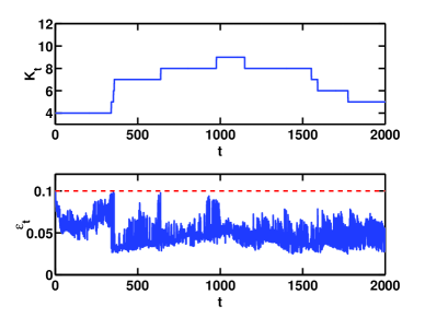
Snapshots of this video at time $t=250$ and $t=1150$ are shown in Figure 1. In this figure, the dashed line corresponds to the true submanifold, the red lines correspond to the estimated union of subsets by MOUSSE, and the $+$ signs correspond to the past 500 samples, with darker colors corresponding to more recent observations. From this video, it is clear that we are effectively tracking the dynamics of the submanifold, and keeping the representation parsimonious so the number of subsets used by our model is proportional to the curvature of the submanifold. As the curvature increases and decreases, the number of subsets used in our approximation similarly increases and decreases. The number of subsets $K_{t}$ and residuals $e_{t}$ as a function of time are shown in Figure 6. The red line in Figure 6 corresponds to $\epsilon$. Note that MOUSSE is able to track the submanifold, in that it can maintain a stable number of leaf nodes in the approximation and meet the target residual tolerance $\epsilon$.

Figure 6: MOUSSE tracking a slowly time-varying submanifold with $D=100$ and $d=1$. The dashed red line depicts the parameter $\epsilon$ used to control approximation errors in the subset tracking.

VI-D Choice of intrinsic dimension $d$

In this section, we study the effect of the choice of the intrinsic dimension $d$ in MOUSSE. We generate a chirp-signal, with ambient dimension $D=100$ and signal intrinsic dimension $d_{0}=2$. Let the two-dimensional parameter be $\theta\triangleq[f_{0},\phi]$, with frequency $f_{0}\in[1,100]$, and phase $\phi\in[0,1]$. Define $v(\theta)\in\mathbb{R}^{D}$ with its $n$-th element

$$[v(\theta)]_{n}=\sin\left[2\pi(f_{0}z_{n}+\frac{k_{t}^{2}}{2}z_{n}^{2}+\phi)\right]$$ (35)

where $z_{n}=10^{-4}n,n=1,2,\dots,100$, corresponds to regularly-spaced points between 0 and 0.01. The parameter $k_{t}$ controls how fast the submanifold changes and is set according to

$$k_{t}=\left\{\begin{array}[]{ll}0.1t,&t=1,2,\dots,1000,\\ 200-0.1t,&t=1001,1002,\dots,2000.\end{array}\right.$$

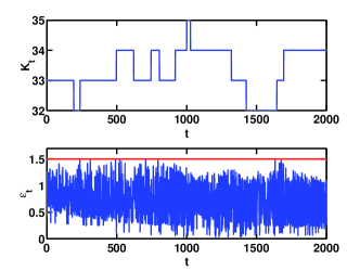
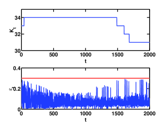
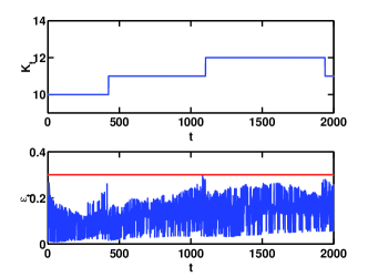
Let $40\%$ of the entries be missing at random. For MOUSEE, we use PETRELS-FO for tracking. We compare the performance of MOUSSE when $d$ is set within the algorithm to be 1, 2, and 3, so there can be a mismatch between the true intrinsic dimension and the assumed $d$. The parameters of MOUSSE set in these scenarios are: for $d=1$: $\epsilon=1.5$, $\mu=0.01$, $\alpha=0.95$; for $d=2$: $\epsilon=0.3$, $\mu=0.01$, $\alpha=0.95$; for $d=3$: $\epsilon=0.3$, $\mu=0.01$, $\alpha=0.95$.

Fig. 7 demonstrates that MOUSSE can track the manifold well when the intrinsic dimension is smaller or equal to the assumed $d$. However, if $d$ is chosen to be too small, the errors are significantly larger and we are forced to use a larger error tolerance $\epsilon$.

(a) $d=1$

(b) $d=2$

(c) $d=3$

Figure 7: Tracking of MOUSSE using $d=1$, $d=2$ and $d=3$, respectively, when the true intrinsic dimension is 2. Red line corresponds to $\epsilon$.

VI-E Change-point detection using MOUSSE

VI-E1 Approximation to ARL

The ARL approximation in (26) assumes $e_{t}$ is Gaussian distributed. We have shown that $e_{t}$ is not exactly Gaussian distributed but close to a Gaussian. Hence, we need to numerically verify the accuracy of (26) for $e_{t}$ generated by MOUSSE. To simulate ARL of the GLR procedure, we generate $10000$ Monte Carlo (MC) trials, each being a noisy realization of the same slowly time-varying submanifold in (33). We then apply MOUSSE to track the submanifold, obtain a sequence of residuals $e_{t}$, apply the GLR change-point detection procedure, and obtain an ARL numerically. We adopt an exponential approximation in [61] to evaluate $\mathbb{E}^{\infty}\{T\}$ efficiently. TABLE I shows the value of $b$ suggested by theory for different ARLs and the value of $b$’s computed via Monte Carlo are very close. For comparison, we also obtain thresholds for change-point detection when a single subspace tracking using PETRELS-FO is employed.

TABLE I: Average run length (ARL) $\mathbb{E}^{\infty}\{T\}$.

ARL	$b$	$b$ MC, $0\%$ data missing		$b$ MC, $20\%$ data missing		$b$ MC, $40\%$ data missing
		MOUSSE	Single Subspace	MOUSSE	Single Subspace	MOUSSE	Single Subspace
1000	3.94	4.81	3.90	4.77	3.91	5.22	3.90
5000	4.35	5.91	4.60	5.66	4.62	6.14	4.59
10000	4.52	6.38	4.91	6.02	4.91	6.49	4.91

VI-E2 Comparison of tracking algorithms for MOUSSE

To estimate the expected detection delay of MOUSSE detecting a change-point, we generate instances where the parameter $\gamma_{t}$ in (30) has an abrupt jump $\Delta_{\gamma}$ at time $t=200$:

$$\gamma_{t}=\left\{\begin{array}[]{ll}0.6-\gamma_{0}t&t=1,2,\dots,199,\\ \gamma_{199}-\Delta_{\gamma}-\gamma_{0}t&t=200,201,\dots,400.\end{array}\right.$$ (38)

We apply the GLR procedures based on $e_{t}$ generated from MOUSSE and single subspace tracking, respectively, and compare the corresponding expected detection delay after $t=200$. We consider two change-point magnitudes: big ($\Delta_{\gamma}=0.05$) and small ($\Delta_{\gamma}=0.03$). The expected detection delays are estimated using 10000 Monte Carlo trials, and are given in Table  II, and Table  III. For comparison, we also obtain thresholds for change-point detection when a single subspace tracking using PETRELS-FO is employed. The threshold $b$’s are chosen according to the Monte Carlo thresholds given in Table I. For example, for the cell corresponding to ARL $=1000$ and $0\%$ missing data in Table II or III, $b$ should be set as $4.55$ for MOUSSE and $4.28$ for the single subspace method. Table II and Table  III demonstrate that change-point detection based on MOUSSE has a much smaller expected detection delay than that based on single subspace tracking.

TABLE II: Detection delay when jump of $\gamma_{t}$ is $\Delta_{\gamma}=0.05$.

ARL	delay, $0\%$ data missing		delay, $20\%$ data missing		delay, $40\%$ data missing
	MOUSSE	Single Subspace	MOUSSE	Single Subspace	MOUSSE	Single Subspace
1000	3.69	91.92	4.02	90.49	5.38	88.72
5000	5.31	104.02	5.48	104.23	7.38	105.05
10000	6.20	98.95	6.13	101.52	8.21	102.99

TABLE III: Detection delay when jump of $\gamma_{t}$ is $\Delta_{\gamma}=0.03$.

ARL	delay, $0\%$ data missing		delay, $20\%$ data missing		delay, $40\%$ data missing
	MOUSSE	Single Subspace	MOUSSE	Single Subspace	MOUSSE	Single Subspace
1000	2.30	54.17	2.39	52.82	2.78	51.53
5000	2.71	80.61	2.76	78.29	3.35	75.47
10000	2.91	90.87	2.94	88.30	3.62	86.48

VI-F Real data

VI-F1 Solar flare detection

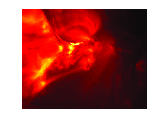
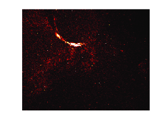
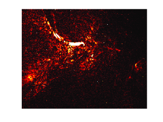
We first consider a video from the Solar Data Observatory, which demonstrates an abrupt emergence of a solar flare . We also display a residual map defined as:

$$\hat{e}_{t}\triangleq(I-U_{j^{*},k^{*},t}U_{j^{*},k^{*},t}^{\#})(x_{t}-c_{j^{*},k^{*},t}),$$ (39)

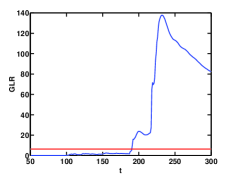
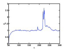
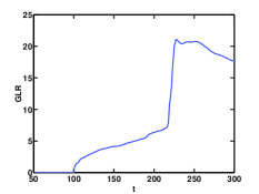
which is useful to localize the solar flare. Here $(j^{*},k^{*})$ denotes the index of the minimum distance subset. The frame is of size $232\times 292$ pixels, which result in $D=67744$ dimensional streaming data. In this video, the normal states are slowly drifting solar flares, and the anomaly is a much brighter transient solar flare. A frame from this dataset during a solar flare around $t=200$ is shown in Figure 8a. In the original images, the background solar images have bright spots with slowly changing shape, which makes detection based on simple background subtraction incapable of detecting small transient flares.

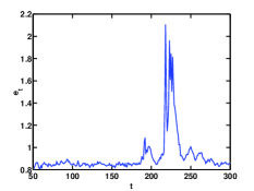
To ease parameter tuning, we scale the pixel intensities by a factor of $10^{-4}$, so the range of data is consistent with our simulated data experiments. The parameters for this example are $d=1$, $\epsilon=0.3$, $\mu=0.3$, and $\alpha=0.85$. Figure 8 demonstrates that MOUSSE can not only detect the emergence of a solar flares, but also localize the flare by presenting $\hat{e}_{t}$, and these tasks are accomplished far more effectively with MOUSSE (even with $d=1$) than with a single subspace. Note that with single subspace tracking, $e_{t}$ is not a stationary timeseries prior to the flare and thus poorly suited for change-point detection. In contrast, with our approach, with $K_{t}$ around $10$, the underlying manifold structure is better tracked and thus yields more stable $e_{t}$ before the change-point and significant change in $e_{t}$ when the change-point occurs.

(a) Snapshot of original SDO data at $t=227$

(b) MOUSSE residual map at $t=227$

(c) Single subspace tracking residual map at $t=227$

(d) $e_{t}$ from MOUSSE

(e) GLR stats from MOUSSE

(f) $e_{t}$ from single subspace tracking

(g) GLR stats from single subspace tracking

Figure 8: Detection of solar flare at $t=227$: (a) snapshot of original SDO data at $t=227$; (b) MOUSSE residual $\hat{e}_{t}$, which clearly identifies an outburst of solar flare; (c) single subspace tracking residual $\hat{e}_{t}$, which gives a poor indication of the flare; (d) $e_{t}$ for MOUSSE which peaks near the flare around $t=227$; (e) the GLR statistic for MOUSSE; (f) $e_{t}$ for single subspace tracking; (g) the GLR statistic for single subspace tracking. Using a single subspace gives much less reliable estimates of significant changes in the statistics of the frames.

VI-F2 Identity theft detection

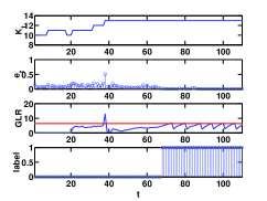
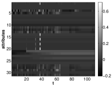
Our second real data example is related to automatic identity theft detection. The basic idea is that consumers have typical spending patterns which change abruptly after identity theft. Banks would like to identify these changes as quickly as possible without triggering numerous false alarms. To test MOUSSE on this high-dimensional changepoint detection problem, we examined the E-commerce transaction history of people in a dataset used for a 2008 UCSD data mining competition. For each person in this dataset, there is a timeseries of transactions. For each transaction we have a 31-dimensional real-valued feature vector and a label of whether the transaction is “good” (0) or “bad” (1). The full dataset was generated for a generic anomaly detection problem, so it generally is not appropriate for our setting. However, some of these transaction timeseries show a clear changepoint in the labels, and we applied MOUSSE to these timeseries. In particular, we use MOUSSE to track the 31-dimensional feature vector and detect a changepoint, and compare this with the “ground truth” changepoint in the label timeseries. In calculating the GLR statistic, we estimate the $\mu_{0}$ and $\sigma_{0}$ of equation 24 from $e_{1},\dots,e_{20}$. After $t=20$, every time the GLR statistic exceeds the threshold $b$ and an changepoint is detected, we “reset” the GLR to only consider $e_{t}$ after the most recently detected changepoint. This allows us to detect multiple change-points in a timeseries.

The effect of our procedure for one person’s transaction history is displayed in Figure 9. We first see that MOUSSE accurately detects a temporally isolated outlier transaction at $t=38$, after which the GLR is reset. After this, while MOUSSE does not generate particularly large spikes in $e_{t}$, the associated GLR statistic shows a marked increase near $t=70$ and hits the threshold at $t=72$ (the threshold corresponds to the Monte Carlo threshold for ARL = 10000 in Table I) when the labels (not used by MOUSSE) change from 0 (good) to 1 (bad). After this the GLR is repeatedly reset and repeatedly detects the change in the statistics of $e_{t}$ from the initial stationary process.

(a) Obtained from MOUSSE

(b) Visualization of time-varying Attributes

Figure 9: Credit card user data experiments. (a) From top to bottom: number of leaf nodes used by MOUSSE; $e_{t}$; GLR statistic (solid blue line) and theoretical threshold $b$ corresponding to ARL = 10000 (dashed red line); ground truth label. Note that the GLR statistic has a false alarm due to an outlier at $t=38$, and it starts increasing at $t=70$ and frequently hits the threshold afterwards due to the changepoint at $t=70$. In this case GLR catches both the outlier and the changepoint. (b) Demonstration of the time-varying $x_{t}$ (user attributes): each column corresponds to the 31-dimensional attribute vector at a given time. The white spots correspond to the outlier at time $t=38$.

VII Conclusions

This paper describes a novel multiscale method for online tracking of high-dimensional data on a low-dimensional submanifold, and using the tracking residuals to perform fast and robust change-point detection. Change-point detection is an important subset of anomaly detection problems due to the ever-increasing volume of streaming data which must be efficiently prioritized and analyzed. The multiscale structure at the heart of our method is based on a geometric multiresolution analysis which facilitates low-complexity piecewise-linear approximations to a manifold. The multiscale structure allows for fast updates of the manifold estimate and flexible approximations which can adapt to the changing curvature of a dynamic submanifold. These ideas have the potential to play an important role in analyzing large volumes of streaming data which arise in remote sensing, credit monitoring, and network traffic analysis.

While the algorithm proposed in this paper has been focused on unions of subsets, an important open question is whether similar techniques could be efficiently adopted based on sparse covariance matrix selection [63, 64]. The resulting approximation space may no longer correspond to a low-dimensional submanifold, but such structures provide good representations of high-dimensional data in many settings, and our future work includes tracking the evolution of a mixture of such structures. Issues related to non-Gaussian observation models, inverse problem settings, dynamical models, and optimal selection of the statistic used for change-point detection (i.e., alternatives to $e_{t}$, as considered in [65]) all pose additional interesting open problems.

Appendix A Optimality of estimate for $c$

We assume that there is complete data, and we restrict our approximation to a single subspace so that $K_{t}=1$. Assume the mean and covariance matrix of the data are given by $c^{\star}$ and $\Sigma^{\star}$, respectively. Assume the covariance matrix has low-rank structure: $\Sigma^{\star}=\mbox{diag}\{\lambda_{1}^{\star},\ldots,\lambda_{D}^{\star}\}$ with $\lambda_{m}=\delta^{\star}$ for $m=d+1,\ldots,D$.

When there is only one subspace and the data are complete, the cost function (3) without the penalty term becomes

$$\min_{U,c}\sum_{i=1}^{t}\alpha^{t-i}\|(I-UU^{\top})(x_{i}-c)\|^{2}.$$ (40)

Recall that the online update for $c_{t}$ is given by $c_{t+1}=\alpha c_{t}+(1-\alpha)x_{t}$, with initialization $c_{0}$. We can prove that this online estimate for $c$ is optimal in the following sense:

Theorem 2

Assume $c^{\star}_{t}$ minimizes (40) at time $t$, $0\leq\alpha<1$, and the initialization is bounded $\|c_{0}\|^{2}<\infty$. Then as $t\rightarrow\infty$, $\|c_{t}-c^{\star}_{t}\|^{2}\rightarrow 0$ in probability. Moreover, assume $x_{t}$’s are i.i.d. with $\mathbb{E}\{x_{t}\}=c^{\star}$, then $\mathbb{E}\{c_{t}\}\rightarrow c^{\star}$, i.e., the estimate is asymptotically unbiased.

Proof: Recall that the online estimate for $c_{t}$ is given by $c_{t+1}=\alpha c_{t}+(1-\alpha)x_{t}$. Hence,

$$c_{t}=(1-\alpha)\sum_{i=1}^{t}\alpha^{t-i}x_{i}+\alpha^{t}c_{0},$$

where the term $\alpha^{t}c_{0}$ is a bias introduced by initial condition $c_{0}$. Let

$$\bar{x}_{t}=\frac{1-\alpha}{1-\alpha^{t}}\sum_{i=1}^{t}\alpha^{t-i}x_{i},\quad S=\sum_{i=1}^{t}\alpha^{t-i}(x_{i}-\bar{x}_{t})(x_{i}-\bar{x}_{t})^{\top}.$$ (41)

By expanding $\|(I-UU^{\top})(x_{i}-c)\|^{2}=\|(I-UU^{\top})(x_{i}-\bar{x}_{t}+\bar{x}_{t}-c)\|^{2}$, and using the fact that $(I-UU^{\top})^{2}=I-UU^{\top}$, we can write the cost function of (40) as

$$\begin{split}&\sum_{i=1}^{t}\alpha^{t-i}\|(I-UU^{\top})(x_{i}-c)\|^{2}\\ =&\sum_{i=1}^{t}\alpha^{t-i}(x_{i}-\bar{x}_{t})^{\top}(I-UU^{\top})(x_{i}-\bar{x}_{t})\\ &+\sum_{i=1}^{t}\alpha^{t-i}(\bar{x}_{t}-c)^{\top}(I-UU^{\top})(\bar{x}_{t}-c)\\ &+2\sum_{i=1}^{t}\alpha^{t-i}(\bar{x}_{t}-c)^{\top}(I-UU^{\top})(x_{i}-\bar{x}_{t}).\end{split}$$ (42)

Since $\bar{x}_{t}$ and $c$ are both independent of $i$, the last term in (42) can be re-written and is equal to zero by the choices of $\bar{x}_{t}$ and $S$:

$$\begin{split}&\sum_{i=1}^{t}\alpha^{t-i}(\bar{x}_{t}-c)^{\top}(I-UU^{\top})(x_{i}-\bar{x}_{t})\\ =&(\bar{x}_{t}-c)^{\top}(I-UU^{\top})\sum_{i=1}^{t}\alpha^{t-i}(x_{i}-\bar{x}_{t})\\ =&(\bar{x}_{t}-c)^{\top}(I-UU^{\top})\left(\sum_{i=1}^{t}\alpha^{t-i}x_{i}-\bar{x}_{t}\sum_{i=1}^{t}\alpha^{t-i}\right)=0,\end{split}$$ (43)

since $\sum_{i=1}^{t}\alpha^{t-i}=(1-\alpha^{t})/(1-\alpha)$. Using the fact that $\mbox{tr}(AB)=\mbox{tr}(BA)$ for two matrix $A$ and $B$, together with (43), the cost function (42) becomes

$$\mbox{tr}[(I-UU^{\top})S]+\frac{1-\alpha^{t}}{1-\alpha}(\bar{x}-c)^{\top}(I-UU^{\top})(\bar{x}-c),$$ (44)

where the first term does not depend on $c$. Since the second term in (44) is quadratic in $c$, it is minimized by choosing $c=\bar{x}_{t}$. Denote this optimal $c$ at time $t$ by $c^{\star}_{t}$.

Hence

$$\|c_{t}^{\star}-c_{t}\|^{2}\leq\left\|\frac{\alpha^{t}}{1-\alpha^{t}}(1-\alpha)\sum_{i=1}^{t}\alpha^{t-i}x_{i}\right\|^{2}+\alpha^{t}\left\|c_{0}\right\|^{2}.$$ (45)

Recall that $c^{\star}$ denote the true mean: $\mathbb{E}\{x_{t}\}=c^{\star}$. As $t\rightarrow\infty$, $\sum_{i=1}^{t}\alpha^{t-i}x_{i}\rightarrow\frac{1}{1-\alpha}c^{\star}$ in probability, the first term in the upper bound (45) tends to 0 in probability. Given bounded $\|c_{0}\|^{2}$, the second term in (45) also tends to 0. Hence our online-estimate $c_{t}$ is asymptotically optimal in that it minimizes (40). Also, $c_{t}$ is asymptotically unbiased, since $\mathbb{E}\{c_{t}\}\rightarrow(1-\alpha)\cdot\frac{1}{1-\alpha}c^{\star}=c^{\star}$.

Appendix B Consistency of estimates of $\Lambda^{\star}$ and $\delta^{\star}$

We assume that there is complete data, and we restrict our approximation to a single subspace so that $K_{t}=1$. In the following, we show that if we have correct $U=U^{\star}$, then for each sample $x_{t}$, its projection $[\beta_{t}]_{m}$ is an unbiased estimator for $\lambda_{m}^{\star}$, and $\|x_{t,\perp}\|^{2}$ is an unbiased estimator for $\sum_{m=d+1}^{D}\lambda_{m}^{\star}$. First note

$$\begin{split}\mathbb{E}\{|[\beta_{t}]_{m}|^{2}\}&=\mathbb{E}\{[\textsf{e}_{m}^{\top}U^{\top}(x_{t}-c)]^{2}\}=\textsf{e}_{m}^{\top}U^{\top}\Sigma^{\star}U\textsf{e}_{m}\\ &=\lambda_{m}^{\star}[U]_{m}^{\top}[U]_{m}=\lambda_{m}^{\star},\end{split}$$ (46)

for $m=1,\ldots,d$, where $\textsf{e}_{m}$ denotes the $m$-th row of an identity matrix. We also have that

$$\begin{split}\mathbb{E}\{\|x_{t,\perp}\|^{2}\}&=\mathbb{E}\{\|(I-UU^{\top})(x_{t}-c)\|^{2}\}\\ &=\mbox{tr}\{(I-UU^{\top})\Sigma^{\star}(I-UU^{\top})\}\\ &=\sum_{m=d+1}^{D}\lambda_{m}^{\star}.\end{split}$$ (47)

Then from the MOUSSE update equations, as $t\rightarrow\infty$

$$\begin{split}\mathbb{E}\{\lambda^{(m)}_{t}\}&=\mathbb{E}\{(1-\alpha)\sum_{i=1}^{t}\alpha^{t-i}|[\beta_{t}]_{m}|^{2}+\alpha^{t}\lambda_{0}^{(m)}\}\rightarrow\lambda_{m}^{\star},\end{split}$$ (48)

for $m=1,\ldots,d$ and

$$\begin{split}\mathbb{E}\{\delta_{t}\}&=\mathbb{E}\{(1-\alpha)\sum_{i=1}^{t}\alpha^{t-i}\|x_{t,\perp}\|^{2}/(D-d)+\alpha^{t}\delta_{0}\}\\ &\rightarrow\frac{1}{D-d}\sum_{m=d+1}^{D}\lambda_{m}^{\star}=\delta^{\star}.\end{split}$$ (49)

Hence our estimators for $\lambda_{m}^{\star}$ and $\delta^{\star}$ are asymptotically unbiased.

Appendix C Proof of Theorem 1

Proof:

From (1) and (9) we have

$$\beta=U^{\top}(v-c)+U^{\top}w,$$ (50)

Note that $U^{\top}w$ is zero-mean Gaussian random vector with covariance matrix $\sigma^{2}U^{\top}U=\sigma^{2}I$.

Next we consider the missing data case. Recall $\mathcal{P}_{\Omega}\in\mathbb{R}^{|\Omega|\times D}$ is a projection matrix. Define $w_{\Omega}=\mathcal{P}_{\Omega}w$. From (9) we have

$$\beta_{\Omega} =U_{\Omega}^{\#}(v_{\Omega}-c_{\Omega})+U_{\Omega}^{\#}w_{\Omega}$$ (51)

Suppose in (1) we write $v-c=p+q$, with $p\in\mathcal{S}$ and $q\in\mathcal{S}^{\perp}$, where $\mathcal{S}^{\perp}$ denotes the orthogonal subspace of $\mathcal{S}$. Hence, $p=UU^{\top}(v-c)$ and $q=(I-UU^{\top})(v-c)$. Let $p_{\Omega}=\mathcal{P}_{\Omega}p$, $q_{\Omega}=\mathcal{P}_{\Omega}q$. Hence, $v_{\Omega}-c_{\Omega}=p_{\Omega}+q_{\Omega}$. Note that

$$U_{\Omega}^{\#}p_{\Omega}= (U_{\Omega}^{\top}U_{\Omega})^{-1}U_{\Omega}^{\top}\mathcal{P}_{\Omega}UU^{\top}(v-c)$$ (52)

$$= (U_{\Omega}^{\top}U_{\Omega})^{-1}U_{\Omega}^{\top}U_{\Omega}U^{\top}(v-c)$$ (53)

$$= U^{\top}(v-c).$$ (54)

So

$$\beta_{\Omega}=U^{\top}(v-c)+U_{\Omega}^{\#}q_{\Omega}+U_{\Omega}^{\#}w_{\Omega}.$$

Hence

$$\begin{split}\|\beta_{\Omega}-\beta\|^{2}&\leq 2\|U_{\Omega}^{\#}q_{\Omega}\|^{2}+2\|U_{\Omega}^{\#}w_{\Omega}-U^{\top}w\|^{2}\\ &=2\|(U_{\Omega}^{\top}U_{\Omega})^{-1}U_{\Omega}^{\top}q_{\Omega}\|^{2}\\ &+2\|[(U_{\Omega}^{\top}U_{\Omega})^{-1}U_{\Omega}^{\top}\mathcal{P}_{\Omega}-U^{\top}]w\|^{2}\end{split}$$

We will bound these two terms separately.

First, note that

$$\|(U_{\Omega}^{\top}U_{\Omega})^{-1}U_{\Omega}^{\top}q_{\Omega}\|^{2} \leq\|(U_{\Omega}^{\top}U_{\Omega})^{-1}\|_{2}^{2}\|U_{\Omega}^{\top}q_{\Omega}\|^{2}$$ (55)

where $\|A\|_{2}$ denotes the spectral norm of matrix $A$. Using [Lemma 2] in [62], we have that with probability $1-\varepsilon$, if $|\Omega|\geq\frac{8}{3}d\textsf{coh}(U)\log(2d/\varepsilon)$,

$$\|U_{\Omega}^{\top}q_{\Omega}\|^{2}\leq(1+\theta)^{2}\frac{|\Omega|}{D}\frac{d}{D}\textsf{coh}(U)\|q\|^{2},$$

where $\theta=\sqrt{2\frac{\max_{n=1}^{D}|[q]_{n}|^{2}}{\|q\|^{2}}\log(1/\varepsilon)}$. Using [Lemma 3] in [62] we have that provided that $0<\ell<1$, with probability at least $1-\varepsilon$,

$$\|(U_{\Omega}^{\top}U_{\Omega})^{-1}\|_{2}\leq\frac{D}{(1-\ell)|\Omega|}.$$ (56)

Combine these with (55), we have that with probability $1-2\varepsilon$,

$$\|(U_{\Omega}^{\top}U_{\Omega})^{-1}U_{\Omega}^{\top}q_{\Omega}\|^{2}\leq\frac{(1+\theta)^{2}}{(1-\ell)^{2}}\cdot\frac{d}{|\Omega|}\cdot\textsf{coh}(U)\|q\|^{2}.$$ (57)

Next we examine the noise term. Define

$$\tilde{w}=[(U_{\Omega}^{\top}U_{\Omega})^{-1}U_{\Omega}^{\top}\mathcal{P}_{\Omega}-U^{\top}]w,$$

which is a zero-mean Gaussian random vector with covariance matrix

$$\Gamma=\sigma^{2}(U_{\Omega}^{\top}U_{\Omega})^{-1}-\sigma^{2}I,$$

where we have used the fact that $\mathcal{P}_{\Omega}\mathcal{P}_{\Omega}^{\top}=I$. Hence we bound the tail of the noise power using Markov inequality:

$$\mathbb{P}(\|\tilde{w}\|^{2}>2\tau^{2}\sigma^{2})\leq e^{-\tau}\mathbb{E}\{e^{\|\tilde{w}\|^{2}/(2\tau\sigma^{2})}\}\leq 2De^{-\tau}$$ (58)

provided that $\tau$ is sufficiently large such that the maximum eigenvalue is smaller than $\tau$: $\lambda_{\max}((U_{\Omega}^{\top}U_{\Omega})^{-1})<\tau$, i.e., $\tau>D/[(1-\ell)|\Omega|],$ by noting that $\lambda_{\max}((U_{\Omega}^{\top}U_{\Omega})^{-1})=\|(U_{\Omega}^{\top}U_{\Omega})^{-1}\|_{2}$. The last equality in (58) is because, under such condition:

$$\begin{split}\mathbb{E}\{e^{\|\tilde{w}\|^{2}/(2\tau\sigma^{2})}\}&=\int e^{\|x\|^{2}/(2\tau\sigma^{2})}(2\pi)^{-D/2}|\Gamma|^{-1/2}e^{-\frac{1}{2}x^{\top}\Gamma^{-1}x}dx\\ &=(2\pi)^{-D/2}|\Gamma|^{-1/2}\int e^{-\frac{1}{2}x^{\top}(\Gamma^{-1}-\tau^{-1}\sigma^{-2}I)x}dx\\ &=|\Gamma|^{-1/2}|\Gamma^{-1}-\tau^{-1}\sigma^{-2}I|^{-1/2}\\ &=|I-\tau^{-1}\sigma^{-2}\Gamma|^{-1/2}\\ &=|(1+1/\tau)I-\tau^{-1}(U_{\Omega}^{\top}U_{\Omega})^{-1}|^{-1/2}\\ &\leq D[(1+1/\tau)-\tau^{-1}\|(U_{\Omega}^{\top}U_{\Omega})^{-1}\|_{2}]^{-1/2}\\ &\leq D\left[(1+1/\tau)-\frac{D}{\tau(1-\ell)|\Omega|}\right]^{-1/2}\\ &=D\left[1-\frac{1}{\tau}(\frac{D}{(1-\ell)|\Omega|}-1)\right]^{-1/2}\end{split}$$

In the last inequality, we have used (56). Note that $D/[(1-\ell)|\Omega|]>1$, and the upper bound in (LABEL:noise_bound_large) is smaller than $2D$ if $\tau>\frac{4}{3}(\frac{D}{(1-\ell)|\Omega|}-1)$ or $\tau>\frac{4}{3}\frac{D}{(1-\ell)|\Omega|}$. Now we set $2De^{-\tau}=\varepsilon$, if $\varepsilon$ is sufficiently small such that $\log(2D/\varepsilon)>\frac{4}{3}\frac{D}{(1-\ell)|\Omega|}$. Hence we have when $|\Omega|>\frac{4}{3}\frac{D}{(1-\ell)\log(2D/\varepsilon)}$, $\|\tilde{w}\|^{2}<\frac{32}{9}\frac{D^{2}\sigma^{2}}{(1-\ell)^{2}|\Omega|^{2}}$ with probability $1-\varepsilon$. Finally, combining (57) and the noise bound above, we obtain the statement in Theorem 1.

∎

References

- [1] M. Basseville and I. V. Nikiforov, Detection of abrupt changes: Theory and applications, Prentice Hall, April 1993.
- [2] H. V. Poor and O. Hadjiliadis, Quickest detection, Cambridge University Press, Dec. 2008.
- [3] A. Lakhina, M. Crovella, and C. Diot, “Diagnosing network-wide traffic anomalies,” in Proc. of SIGCOMM, 2004.
- [4] M. Raginsky, R. Willett, C. Horn, J. Silva, and R. Marcia, “Sequential anomaly detection in the presence of noise and limited feedback,” IEEE Trans. Info. Theory, vol. 58, no. 8, pp. 5544 – 5562, Aug. 2012.
- [5] K.-C. Lee and D. Kriegman, “Online learning of probabilistic appearance manifolds for video-based recognition and tracking,” in Proc. of CVPR, 2005, pp. 852 – 859.
- [6] Youngser Park, Carey E. Priebe, and Abdou Youssef, “Anomaly detection in time series of graphs using fusion of graph invariants,” arXiv:1210.8429, 2012.
- [7] M. Qu, F. Y. Shih, J. Jing, and H. Wang, “Automatic solar filament detection using image processing techniques,” Solar Physics, , no. 1-2, pp. 119–135, 2005, DOI: 10.1007/s11207-005-5780-1.
- [8] J. Kappenman, “A perfect storm of planetary proportions,” IEEE Spectrum, vol. 49, no. 2, pp. 26 – 31, Feb. 2012.
- [9] J. B. Tenenbaum, V. de Silva, and J. C. Langford, “A global geometric framework for nonlinear dimensionality reduction,” Science, vol. 290, no. 5500, pp. 2319–2323, 2000.
- [10] S. Roweis and L. Saul, “Nonlinear dimensionality reduction by locally linear embedding,” Science, vol. 22, no. 5500, pp. 2323–2326, 2000.
- [11] M. Belkin, Problems of Learning on Manifolds, Ph.D. thesis, University of Chicago, 2003.
- [12] J. A. Costa and A. O. Hero, “Geodesic entropic graphs for dimension and entropy estimation in manifold learning,” IEEE Trans. Sig. Proc., vol. 25, no. 8, pp. 2210–2221, 2004.
- [13] M. Belkin, P. Niyogi, and V. Singhwani, “Manifold regularization: A geometric framework for learning from labeled and unlabeled examples,” J. of Machine Learing Res., vol. 7, pp. 2399 – 2434, 2006.
- [14] M. B. Wakin, “Manifold-based signal recovery and parameter estimation from compressive measurements,” submitted, 2009.
- [15] W. Allard, G. Chen, and M. Maggioni, “Multi-scale geometric methods for data sets II: Geometric multi-resolution analysis,” App. and Comp. Harmonic Ana., vol. 32, no. 3, pp. 435 – 462, May 2011.
- [16] Sofia Karygianni and Pascal Frossard, “Tangent-based manifold approximation with locally linear models,” arXiv:1211.1893, 2012.
- [17] L. Balzano, R. Nowak, and B. Recht, “Online identification and tracking of subspaces from highly incomplete information,” in Proc. Allerton Conf. on Comm., Control and Comp., Sept. 2010, pp. 704 – 711.
- [18] Y. Chi, Y. C. Eldar, and R. Calderbank, “PETRELS: Subspace estimation and tracking from partial observations,” in IEEE Int. Conf. on Acoustics, Speech and Sig. Proc. (ICASSP), 2012.
- [19] Y. Chi, Y. C. Eldar, and R. Calderbank, “Petrels: Parallel estimation and tracking of subspace by recursive least squares from partial observations,” submitted to IEEE Trans. Sig. Proc., arXived., July 2012.
- [20] Carey Priebe and David Marchette, “Adaptive mixture density estimation,” Pattern Recognition, vol. 26, no. 5, pp. 771 – 785, May 1993.
- [21] M. Kristan, D. Skočaj, and A. Leonardis, “Online kernel density estimation for interactive learning,” Image Vision Comput., vol. 28, no. 7, pp. 1106–1116, 2010.
- [22] M. Kristan, A. Leonardis, and D. Skočaj, “Multivariate online kernel density estimation with gaussian kernels,” Pattern Recognition, vol. 44, pp. 2630–2642, 2011.
- [23] Ph. Rigollet and A. B. Tsybakov, “Linear and convex aggregation of density estimators,” Math. Methods Statist., vol. 16, no. 3, pp. 260–280, 2007.
- [24] R. S. G. Mahapatruni and A. G. Gray, “Cake: Convex adaptive kernel density estimation,” J. of Machine Learing Res. - Proceedings Track, vol. 15, pp. 498–506, 2011.
- [25] John Lafferty and Larry Wasserman, “Rodeo: Sparse, greedy nonparametric regression,” Ann. Stat., vol. 36, no. arXiv:0803.1709. IMS-AOS-AOS0318. 1, pp. 28–63, Mar 2008.
- [26] G. McLachlan and D. Peel, Finite Mixture Models, Wiley, 2000.
- [27] Q. Li, Estimation of Mixture Models, Ph.D. thesis, Yale University, 1999.
- [28] Q. Li and A. Barron, Advances in Neural Information Processing Systems 12, chapter Mixture Density Estimation, MIT Press, 2000.
- [29] Jacob Goldberger and Sam Roweis, “Hierarchical clustering of a mixture model,” in Neural Info. Proc. Sys. (NIPS), 2005.
- [30] G. McLachlan and T. Krishnan, The EM Algorithm and Extensions, Wiley, New York, 1997.
- [31] Arnaud Declercq and Justus H. Piater, “Online learning of Gaussian mixture models: A two-level approach,” in Proc. of the 3rd Int. Conf. on Computer Vision Theory and App. (VISAPP), 2008.
- [32] D. Bezier, “BAE to develop surveillance system,” The Washington Post, 2007, http://www.washingtonpost.com/wp-dyn/content/article/2007/11/11/AR2007111101348.html, retrieved 3-20-2012.
- [33] D. Hambling, “Special forces’ gigapixel flying spy sees all,” 2009, http://www.wired.com/dangerroom/2009/02/gigapixel-flyin/.
- [34] NASA, “SDO instruments,” Retrieved 7-30-2012, http://sdo.gsfc.nasa.gov/mission/instruments.php.
- [35] V. Mahadevan, W. Li, V. Bhalodia, and N. Vasconcelos, “Anomaly detection in crowded scenes,” in IEEE. Conf. on Comp. Vision and Pattern Rec., San Francisco, 2010, pp. 1975 – 1981.
- [36] X. Hou and L. Zhang, “Saliency detection: A spectral residual approach,” in In IEEE Conference on Computer Vision and Pattern Recognition (CVPR07). IEEE Computer Society, 2007, pp. 1–8.
- [37] H. J. Seo and P. Milanfar, “Static and space-time visual saliency detection by self-resemblance,” J. of Vision, vol. 9, no. 12, pp. 1–27, Nov. 2009.
- [38] K. Kennedy, B. Mac Namee, and S. J. Delany, “Using semi-supervised classifiers for credit scoring,” 2012, http://www.palgrave-journals.com/jors/journal/vaop/ncurrent/abs/jors201130a.html.
- [39] T. Ahmed and M. Coates, “Multivariate online anomaly detection using kernel recursive least squares,” in Proc. IEEE Infocom, 2007.
- [40] A. S. Polunchenko, A. G. Tartakovsky, and N. Mukhopadhyay, “Nearly optimal change-point detection with an application to cybersecurity,” submitted to Sequential Analysis, Mar. 2012.
- [41] N. Patwari, A. O. Hero, III, and A. Pacholski, “Manifold learning visualization of network traffic data,” in Proc. ACM SIGCOMM workshop on mining network data (MineNet), 2005, pp. 191 – 196.
- [42] D. Siegmund and E. S. Venkatraman, “Using the generalized likelihood ratio statistic for sequential detection of a change-point,” Annals of Stat., vol. 23, no. 1, pp. 255 – 271, 1995.
- [43] D. Donoho, “Cart and best-ortho-basis selection: A connection,” Annals of Stat., vol. 25, pp. 1870–1911, 1997.
- [44] Y. Chi, Y. C. Eldar, and R. Calderbank, “PETReLS: Subspace estimation and tracking from partial observations,” in Int. Conf. on Acoustic, Speech, and Sig. Proc. (ICASSP), Mar. 2012.
- [45] K. Abed-Meraim, A. Chkeif, Y. Hua, and S. Attallah, “On a class of orthonormal algorithms for principal and minor subspace tracking,” J. of VLSI Sig Proc., vol. 31, pp. 57–70, 2002.
- [46] R. Meir, “Nonparametric time series prediction through adaptive model selection,” Machine Learning, vol. 39, pp. 5–34, 2000.
- [47] L. Breiman, J. Friedman, R. Olshen, and C. J. Stone, Classification and Regression Trees, Wadsworth, Belmont, CA, 1983.
- [48] R. Willett and R. Nowak, “Multiscale Poisson intensity and density estimation,” IEEE Trans. Info. Theory, vol. 53, no. 9, pp. 3171–3187, 2007.
- [49] A. Barron, J. Rissanen, and B. Yu, “Minimum description length principle in coding and modeling,” IEEE Trans. Info. Theory, vol. 44, no. 6, pp. 2743–2760, October 1998.
- [50] N. Merhav and M. Feder, “Universal prediction,” IEEE Trans. Info. Theory, vol. 44, no. 6, pp. 2124–2147, October 1998.
- [51] S. Haykin, Adaptive Filter Theory, Prentice Hall, 4th edition, 2001.
- [52] E. S. Page, “Continuous inspection scheme,” Biometrika, vol. 41, no. 1/2, pp. 100 – 115, June 1954.
- [53] G. Lorden, “Procedure for reacting to a change in distribution,” Ann. Math. Statist., vol. 42, pp. 1897 – 1908, 1971.
- [54] A. N. Shiryayev, “On optimal method in earliest detection problems,” Theory Probab. Appl., vol. 8, pp. 26 – 51, 1963.
- [55] S. W. Roberts, “A comparison of some control chart procedures,” Technometrics, vol. 8, pp. 411 – 430, 1966.
- [56] A. Polunchenko and A.G. Tartakovsky, “State-of-the-art in sequential change-point detection,” Methodology and Computing in Applied Probability, vol. 14, no. 3, pp. 649–684, 2012.
- [57] M. Pollak, “Optimal detection of a change in distribution,” Ann. Stat., vol. 13, pp. 206 – 227, 1985.
- [58] M. Pollak and A.G. Tartakovsky, “Optimality of the Shiryaev-Roberts procedure,” Statistica Sinica, vol. 19, no. 4, pp. 1729–1739, 2009.
- [59] M. Pollak and D. Siegmund, “Sequential detection of a change in a normal mean when the initial value is unknown,” Annals of Stats., vol. 19, no. 1, pp. 394 – 416, 1991.
- [60] D. Siegmund, Sequential Analysis: Test and Confidence Intervals, Springer, Aug. 1985.
- [61] Y. Xie and D. Siegmund, “Sequential multi-sensor change-point detection,” submitted to Annals of Statis, June 2012.
- [62] L. Balzano, B. Recht, and R. Nowak, “High-dimensional matched subspace detection when data are missing,” in IEEE Int. Sym. Info. Theory, June 2010, pp. 1638 – 1642.
- [63] A. d’Aspremont, O. Banerjee, and L. El Ghaoui, “First-order methods for sparse covariance selection,” SIAM. J. Matrix Anal. & Appl, vol. 30, no. 56, 2008.
- [64] S. M. Kakade, O. Shamir, K. Sridharan, and A. Tewari, “Learning exponential families in high-dimensionals: Strong convenxity and sparsity,” in Proc. of Int. Conf. on Artificial Intel. and Stats, 2010, pp. 381 – 388.
- [65] Y. Xie and D. Siegmund, “Parallel sequential multisensor changepoint detection,” in Joint Stats. Meeting (JSM), San Diego, 2012.