Vacuum Kundt waves
Abstract.
We discuss the invariant classification of vacuum Kundt waves using the Cartan-Karlhede algorithm and determine the upper bound on the number of iterations of the Karlhede algorithm to classify the vacuum Kundt waves [11, 15]. By choosing a particular coordinate system we partially construct the canonical coframe used in the classification to study the functional dependence of the invariants arising at each iteration of the algorithm. We provide a new upper bound, , and show that this bound is sharp by analyzing the subclass of Kundt waves with invariant count beginning with (0,1,…) to show that the class with invariant count exists. This class of vacuum Kundt waves is shown to be unique as the only set of metrics requiring the fourth covariant derivatives of the curvature. We conclude with an invariant classification of the vacuum Kundt waves using a suite of invariants.
1. Introduction
The Kundt waves were originally defined by Kundt in 1961 [1], as a special subcase of the class of pure radiation solutions of Petrov type III or higher and Plebanski-Petrov (PP) type O or vacuum admitting a non-twisting, non-expanding null congruence, , that is
These conditions restrict the Petrov type for the plane-fronted waves to Petrov type N or O. Choosing Kundt coordinates, the metric for the Kundt waves is
| (1) |
where are null coordinates, and are complex coordinates for the transverse space[2].
All polynomial curvature invariants, built from contracting the Riemann tensor and covariant derivatives with each other, vanish for these spacetimes. Thus, the plane-fronted belong to the collection of spacetimes where all polynomial curvature invariants vanish [3]; this is, in turn, a subclass of the spacetimes in which all polynomial curvature invariants are constant [4]. These spaces have been explored in four dimensions and were shown to belong to the class of degenerate Kundt metrics [7]. These are the Kundt metrics where the frame used to classify the Riemann tensor (i.e., Petrov or Riemann type [6]) and the kinematic frame are aligned; i.e., they are the same. It is expected that this is the case in higher dimensions as well [8, 7].
For a given spacetime in four dimensions, a spacetime is either uniquely determined by its polynomial scalar curvature invariants, is a (locally) homogeneous space, or is a degenerate Kundt spacetime [7]. For the degenerate Kundt spacetimes the equivalence problem is particularly relevant, given that one cannot determine the inequivalence of two metrics of this class by comparing polynomial scalar curvature invariants [3, 4, 5]. To invariantly classify these spacetimes, one must use an alternative tool, the Karlhede algorithm, which utilizes the Cartan equivalence method [9] adapted to the case of Lorentzian manifolds [10] .
The first and second stages of the Karlhede algorithm were analyzed for all type N vacuum spacetimes with by Collins [11], who produced a theoretical upper bound on the highest order, q, of the covariant derivatives of the curvature tensor required for each of the various subclasses of the type N spacetimes. Interestingly, this gives a hard upper bound for the spacetimes [3, 4], as the pp-waves and vacuum Kundt waves make up the entirety of type N spacetimes [12, 3, 14]. Collins has shown that the pp-waves require while the vacuum Kundt waves need at most . Recently it has been shown that the pp-wave upper bound is sharp [13], and that the actual Kundt-wave’s upper bound is five [15]. However, in 2000, Skea produced a non-vacuum Kundt wave in which , suggesting that there might be vacuum solutions for which [16].
In this paper, we discuss the upper bound for the vacuum Kundt waves in the Karlhede algorithm or, equivalently, the highest order, q, covariant derivative of the curvature required to invariantly classify these spaces. We show that the upper bound may be lowered to be less than or equal to four by exploring all possible outcomes of the Karlhede algorithm (see figures (2), (3) and (4)). Out of all possible invariant counts only one actual vacuum Kundt wave may be integrated; namely, the class with invariant count . Due to the exhaustive nature of this analysis we examine the remaining branches of possibilities in the algorithm to produce an invariant classification of all vacuum Kundt waves. This classification is summarized in two tables describing each of the non-diffeomorphic vacuum Kundt wave metrics arising by the choice of the metric function . We present twelve propositions relating the form of the metric function to the essential Cartan invariants characterizing each spacetime in the first three appendices. The final appendix contains all of the potential subcases of the Karlhede algorithm applied to the vacuum Kundt wave spacetimes prior to examining the geometric structure of these spacetimes.
2. Geometric Structure of the Vacuum Kundt Waves
If we wish to preserve the form of the metric, the permitted coordinate transformations are [3]:
| (2) | |||
where is a real constant and is an arbitrary real function. Taking the metric (1), we work with the Newman-Penrose formalism [18] to calculate the non-vanishing curvature components of the Ricci () and Weyl ) spinors, respectively:
To satisfy the vacuum conditions, must be harmonic and real-valued; as in the pp-waves, this will be the real part of an analytic function, . To examine the geometric structure of these spaces, we work with the class of coframes in which . These are found by applying an appropriate spin and boost to the natural metric coframe.
Without imposing the vacuum condition, the non-vanishing Bianchi identities imply the relationship between the spin-coefficients and the components of the Ricci and Weyl spinors [18] and their frame derivatives :
Imposing the vacuum conditions, we see that . The non-vanishing Newman-Penrose field equations for the vacuum Kundt waves are:
| (3) | |||
| (4) | |||
| (5) | |||
| (6) | |||
| (7) | |||
| (8) | |||
| (9) | |||
| (10) | |||
| (11) | |||
| (12) | |||
| (13) | |||
| (14) | |||
| (15) |
while the commutator relations are
The benefit of working in the class of coframes for which becomes apparent once one takes frame derivatives of the Weyl tensor, as only spin-coefficients and their derivatives appear as components of the Weyl tensor and its covariant derivatives. To illustrate, the first order derivatives of the Weyl tensor are
At first order, one still has 2 degrees of frame freedom, using null rotations with complex parameter , which affects the first order invariant and leaves and unchanged:
| (16) |
If it is always possible to set . However, if equality holds, only one degree of freedom can be fixed, and there are three subcases for the form of [11]:
-
•
: ;
-
•
: ;
-
•
: or = 0, but not both.
Without fixing the frame freedom, the non-zero second order derivatives of the Weyl tensor are:
If , it is always possible to fix the last parameter of the frame freedom to fix so that . Manipulating the spin-coefficients and the remaining degrees of freedom, Collins produced a theoretical upper bound for these spaces [11], requiring at most six covariant derivatives. This bound was lowered to five covariant derivatives by Machados Ramos and Vickers [15] using the generalized GHP formalism. In both papers a particular choice of coordinates was avoided so that these bounds were not shown to be sharp.
3. An Alternative Proof That The Upper Bound for the Karlhede Algorithm is Less than Six
The Karlhede algorithm terminates if and only if the dimension of the isotropy group and number of functionally independent invariants are unchanged from one iteration to the next. Using the invariant count notation, it is possible to map out all possibilities for the Karlhede algorithm. The case where the invariant count begins with is not permitted as the invariant must be non-constant at first order; if we assume is a constant we find from (13) and (14) that , which cannot be true since we are studying the vacuum Kundt waves. With this in mind, it is easily shown that there is only one scenario where at most, (0,1,1,2,3,4,4)111This notation is adopted in Appendix D to summarize possible states of the Karlhede algorithm compactly..
This invariant count would occur for the class of vacuum Kundt waves in which at first order only one functionally independent invariant appears and further that . By choosing a particular coordinate system we may produce differential constraints on the metric function by imposing the vanishing of the wedge products of the differentials of the spin-coefficients of , and their conjugates. As the spins and boosts have been fixed to set , and since these two invariants and are unchanged under the remainder of the isotropy group (null rotations about ), these are already Cartan invariants. With a little effort and a change of coordinates we intend to prove the following theorem:
Theorem 3.1.
The vacuum Kundt waves require at most iterations of the Karlhede algorithm to completely classify the spacetimes.
To this end we introduce a new complex coordinate . Relative to this new coordinate system, and we find a differential constraint for the metric function ,
| (17) |
The metric coframe becomes:
| (18) | |||||
In these coordinates the non-zero component of the Weyl tensor is now
Applying a spin and boost with to the metric coframe (18), we produce a new coframe:
| (19) |
Relative to this coframe, the non-vanishing Weyl tensor component has been normalized and the spin-coefficients and are already Cartan invariants as they are unaffected by the remaining isotropy.
By direct calculation we produce the following spin-coefficients relative to this coframe:
Proposition 3.2.
The spin-coefficients relative to the class of coframes (19), in which , may be expressed as
| (20) | |||
Before we fix any more frame freedom to set all or a part of to zero, we may determine the explicit form of the metric function for the class of vacuum Kundt waves where only one functionally independent invariant arises in the set :
Lemma 3.3.
Those spacetimes in which the spin-coefficients , and are functionally dependent on one invariant will have the following form for the metric function :
| (21) |
Relative to the coordinates , the Cartan invariants and are now
| (22) |
Proof.
Taking in (20), we calculate the double wedge product of and to get,
Requiring that this must vanish gives a set of equations: . Thus is of the form
| (23) |
Plugging this into the expressions for and in (20) we recover (22), and then solving for and noting that we may integrate twice to recover the function in the usual coordinate system. ∎
The vacuum Kundt wave spacetimes with this property will potentially contain at most two functionally independent invariants at first order: and which will simplify the search for those vacuum Kundt waves with only one functionally independent invariant at first order. Furthermore, as the necessary conditions for fixing the remaining isotropy is dependent on the Cartan invariants and we may use the explicit form of these invariants from lemma 3.3 to show all isotropy may be fixed at first order (i.e., ) and that no vacuum Kundt wave requires in the algorithm.
Corollary 3.4.
The invariant count cannot occur in the Karlhede classification of the vacuum Kundt waves.
Proof.
From lemma 3.3 we calculate the equality using equation (22). We assume the equality holds and multiply both sides by , so that . Expanding this we have:
Using the coordinates and simplifying we find the following
Differentiating with respect to or implies that which cannot happen as must be non-zero. This is a contradiction and so . ∎
As this is the only permitted state in the Karlhede algorithm for the vacuum Kundt waves with , and this case cannot occur, we conclude that the upper-bound for the vacuum Kundt waves may be lowered to less than or equal to five.
4. Reducing the Upper Bound to Less than Five
The goal of this section is to provide the necessary lemmas to prove the following theorem:
Theorem 4.1.
The vacuum Kundt wave spacetimes require, at most, four derivatives (i.e., ) to classify these spaces using the Karlhede algorithm.
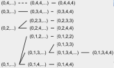
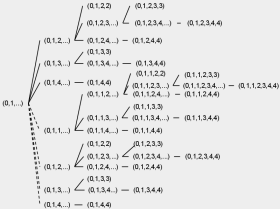
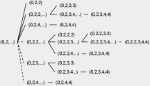
To study the sharpness of the upper bound, we examine the possible iteration scheme for the Karlhede algorithm applied to the vacuum Kundt waves as tree diagrams. This may be done exhaustively for the cases where there are at least one invariant at the first iteration of the algorithm.
Lemma 4.2.
The vacuum Kundt wave spacetimes for which the Karlhede algorithm requires five iterations have invariant counts
| . |
Proof.
The trees for the various possibilities are included in Appendix D. ∎
To prove theorem 4.1 we must examine the constraints on the vacuum Kundt waves to produce the invariant counts in lemma 4.2. To do so we break up the analysis into two subsections to examine the distinct subclasses of vacuum Kundt waves with either one or two functionally independent invariants appearing at first order.
4.1. Vacuum Kundt waves with
Applying the results of lemma 3.3 and corollary 3.4, we are able to say something about the upper bound in the first case, as the invariant coframe is produced from (19) by making a null rotation (16) to set . We must determine the form of the parameter for the null rotation taking the coframe (19) to the invariant coframe required for the Karlhede algorithm:
| (24) |
To achieve this, we equate (16) to zero and solve for ,
| (25) |
Using the dual of the invariant coframe, , we may compute the second order Cartan invariants as the frame derivatives of the first order Cartan invariants along with the following transformed spin-coefficients:
| (26) |
These remaining invariants are expressed in terms of the coframe (19), the original spin-coefficients (20), and the frame derivatives of relative to the original coframe (19) with :
| (27) | |||||
Noting that in (20) and subtracting from , it is clear that is an invariant; a quick calculation confirms that it is functionally dependent on and its conjugate. We now examine the second order invariant arising from the frame derivative of ; removing all terms that are functionally dependent on leaves the helpful invariant:
| (28) |
As , the remaining invariants at second order may be simplified to the spin-coefficients and . These spin-coefficients involve and the remaining frame derivatives of this function:
| (29) |
where is the following complex rational function of ,
Combining these functions, it is clear that both and are expressed entirely in terms of and .
At this point we are able to prove that at second order, at least two functionally independent invariants are produced if we wish to produce a vacuum Kundt wave with in the algorithm.
Lemma 4.3.
All vacuum Kundt waves with the metric function of the form (21) and an invariant count starting with in the Karlhede algorithm must end at third order; i.e., with an invariant count .
Proof.
The last invariant given in gives one new candidate for a functionally independent invariant: . Applying the transformation law for it is seen that we may remove the majority of the terms in and instead study the new invariant: As , we may always combine this and its conjugate to produce a simpler invariant
| (30) |
Denoting and we remove those terms in that are functionally dependent on and its conjugate to produce a new invariant:
| (31) | |||
Multiplying to and taking the difference of this new quantity with its conjugate,
then by removing this term from leaves
| (32) |
We calculate the triple wedge product of this invariant with the previous invariants. The coefficients of the triple wedge product relative to the coordinate 3-form basis are extensive. However, only one is necessary if we wish that the triple wedge product vanishes, the vanishing of the coefficient yields
As is a linear function in , must vanish and hence as well.
These constraints cause to vanish and so we work with the remaining invariant ,
Using the same procedure of equating the triple wedge product of , and , we examine the -component, equating this to zero we find a differential equation:
Integrating we find that and hence
To continue, we eliminate the parts of this invariant expressed in terms of previous invariants, by denoting . We take the triple wedge product of this invariant with and to produce the following equation in the component which must vanish: . Denoting , the remaining invariant becomes . If we wish to have only two functionally independent invariants at second order, . This is generically the case; if we may always set to zero using the coordinate transformation, (2) of the form: . Applying this transformation, the analytic function becomes
At third order there are no candidates for a third functionally independent invariant as all frame derivatives of produce invariants expressed in terms of the previous invariants. The Karlhede algorithm terminates with an invariant count . ∎
Thus we have shown that vacuum Kundt waves with an invariant count of in the Karlhede algorithm cannot occur as the metrics with invariant counts starting with must have at the next order.
4.2. Vacuum Kundt waves with
To begin, we prove a more general result for the vacuum Kundt waves with invariant count and .
Lemma 4.4.
For those vacuum Kundt waves with at least one functionally independent invariant appearing at first order and such that then , .
Proof.
Expanding the conjugate of using (20) we find
Upon simplification this leads to the equation
A contraction arises here, as we may differentiate with respect to giving . ∎
Recalling the comment after equation (16) there are three cases to consider depending on the phase of the conjugate of . This lemma implies that the first two cases where cannot occur.
To start narrowing the possibilities for we consider the wedge products of invariants built out of , and their conjugates. As , and are both invariants it will be helpful to consider the triple wedge product:
| (33) |
Alternatively, using the invariant , we have another equation as the coefficient of the triple wedge product:
| (34) |
Equating these two wedge products to zero, we have sufficient information to solve for in the vacuum Kundt wave metrics with invariant count , and hence narrow down the possibilities for those spacetimes with invariant count .
Lemma 4.5.
The vacuum Kundt wave metrics for which the triple wedge product of , and their conjugates vanish have the following form:
| (35) | |||||
| (36) | |||||
| (37) |
Proof.
Equating equations (33) and (34) to zero, we have two differential equations for and its conjugate. There will be four cases depending on whether and are zero or not.
Case 1 - :
Equation (33) vanishes entirely while (34) implies , so that
| (38) |
Solving for and integrating we find the form (35).
Case 2 - :
Here the constraints immediately imply
| (39) |
Solving for and integrating yields the analytic function (36).
Case 3 - :
These assumptions cause (34) to become , implying takes the form:
| (40) |
Solving for and assuming , the expression becomes,
As and are arbitrary functions of , we make one more assumption, . Integrating twice yields the desired metric function (37).
Case 4 -
Re-arranging the functions we find
which is equivalent to . Integrating with respect to yields . Substituting this into (34) we find that , so that takes the form
| (41) |
Solving for and assuming and , we integrate twice to find
Any metric with a function of this form may be transformed into one of the form (37) using the transformation The division of the case with cannot be made by vanishing or not; it is a coordinate-dependent distinction. ∎
These metrics do not yet belong to the class as we must determine whether may be set to zero or not. If is non-zero, the various triple wedge products involving with , and their conjugates give further conditions on the metric function . By lemma 4.4 we see that and hence we may eliminate the real or imaginary part of but not both as the ratio of the real part to the imaginary part of the quantity, , is [11].
Opting to eliminate the real part of , we note that the purely imaginary invariant is invariant under any null rotation preserving . Thus, without fixing the frame any further, the transformed scalar is a Cartan invariant:
We may consider the triple wedge product of the differentials of three invariants constructed from , , and their complex conjugates to determine the feasibility of the vacuum Kundt waves with invariant count .
Lemma 4.6.
The class of vacuum Kundt waves with an invariant count beginning with (0,2,2,…) and cannot occur.
Proof.
Taking the triple wedge product of the invariants , and , we examine the coefficients of , and , equating these coefficients to zero we find two constraints:
Immediately we see that the metric function must be of the form (36) with the corresponding form of given in (39). Expressing and in terms of this function the required equality implies
where with either or non-zero. Expanding and differentiating twice with respect to we find a constant that must vanish:
This produces a contradiction as we have assumed , thus there are no vacuum Kundt wave spacetimes with an invariant count where the first order Cartan invariants satisfy . ∎
We have shown that the collection of vacuum Kundt waves must have either an invariant count with all isotropy fixed at first order, or an invariant count of with implying all isotropy is fixed at second order. Regardless of either case, none of the potential spacetimes arising from these subclasses produce an invariant count with . This lemma completes the proof of theorem 4.1 as we have shown the two possibilities for the Karlhede algorithm requiring cannot occur.
5. Sharpness of the Upper Bound
In this section we will show that the new upper bound is indeed sharp by producing an explicit metric function .
Theorem 5.1.
The vacuum Kundt waves with invariant count are of the form
where and are non-constant and satisfy either
| (42) | |||
Proof.
To prove this fact, we calculate the quadruple wedge product of the differentials of , and two new invariants arising in where the invariant in (32) is now denoted as , and arises from the imaginary part of ,
| (43) | |||
In these coordinates, the invariants are a bit complicated; one may make a coordinate transformation to remove in the function in (21). Applying the transformation (2): . Relabeling the arbitrary functions and , the analytic function becomes
| (44) |
Dropping the primes and repeating the calculations in lemma 3.3 and subsection (4.1) with this new function, one finds that and are now
| (45) |
From the quadruple wedge product we find the sole coefficient yields three essential equations whose vanishing is necessary and sufficient for the 4-form to vanish:
To solve these equations we must consider two cases depending on whether or not. In the case that does vanish, we find that may be expressed in terms of derivatives , an arbitrary function:
| (46) |
While if and arbitrary, we find that
| (47) |
The choice of these functions is reflected in the structure of the invariants. Supposing that , we may express in terms of ,
While if we find that and may be expressed in terms of ,
| (48) |
Regardless of whether or not, the third second order invariant arising here is of the form
The frame derivatives of this invariant produce only one new functionally independent invariant,
To determine the full class of vacuum Kundt waves, we must avoid those functions which give the invariant count , this can only happen if is constant or when it satisfies the following differential equation,
by integrating one finds that .
In the case that is constant, all of the metric functions in (44) are independent of and hence this is a metric with no -dependence. In the other case, we may make a coordinate transformation: Dropping the primes, in these new coordinates the metrics with are now of the form
| (49) |
while those metrics with are
| (50) |
From [19] we conclude these are all spacetimes. ∎
We conclude this section with the result that the sharpness of the upper bound has been confirmed.
6. Uniqueness of the Vacuum Kundt Waves with in the Karlhede Algorithm
From the invariant count trees in Appendix D, the remaining possibilities for vacuum Kundt waves to attain outside of the class with are: and . It was proven in section 4 that the first four cases cannot occur due to lemma 4.3 and lemma 4.5, respectively. The last case may be ignored by applying lemma 7.2 to show that the vacuum Kundt waves with invariant count cannot occur.
Thus we need only investigate the existence of the vacuum Kundt waves to determine the uniqueness of the vacuum Kundt waves with . In this case may be set to zero and the invariant coframe is entirely fixed. To continue, we examine the second order invariants arising from the frame derivatives (24) applied to the simpler set of invariants:
By direct calculation we may prove the following proposition.
Proposition 6.1.
For all vacuum Kundt waves with , the second order Cartan invariants with no functional dependence on the previous invariants consist of the spin-coefficients , , : and the frame derivatives:
In the coordinate system with , these invariants take the form:
To inquire into the uniqueness of the vacuum Kundt waves, we classify the vacuum Kundt waves with invariant count beginning with . In order to identify this subclass we consider the quadruple wedge products of and . If there are only three functionally independent invariants at second order, all twelve quadruple wedge products must vanish.
Lemma 6.2.
The vacuum Kundt wave metrics with an analytic function of the form (35):
have the invariant count .
Proof.
To start, we make a coordinate transformation to remove the imaginary part of in (35) via the transformation Writing , we find that the first order invariants arising from and are
| (51) |
As in order to avoid metrics of the form (36), we take its inverse locally and express all other functions of in terms of it.
Thus we are left with and as invariants. Noting that , where is
Removing the -dependent piece, we may solve for as a third functionally independent invariant. Taking in proposition 6.1 we eliminate all terms dependent on and leaving as the last invariant at second order to complete the set with the spin-coefficients at first and second order acting as the classifying manifold along with the frame derivatives of and . ∎
With this case eliminated, we may consider those vacuum Kundt waves with . The vanishing of the quadruple wedge products produce six equations
| (52) |
Lemma 6.3.
The vacuum Kundt wave metrics with analytic function of the form (36):
have the invariant count except in the subclass of these metrics with
which have the invariant count
Proof.
We first examine the possibility of invariant counts of the form using the metric function (36). In this case the function is , we find that the first order invariants arising from and are
| (53) |
At second order, , thus there is only one quadruple wedge product giving constraints on the metric functions. Mutiplying and adding it to gives a useful invariant
To calculate the wedge product we scale and and use the following quantities:
Substituting into equation (52) and differentiating the whole expression by we find the simpler constraint, , from which we find that implying that and are the only first order invariants.
Returning to the original invariants and , substituting into equation (52) and denoting we find that this becomes,
As before, setting this equation to zero we find that . Substituting the form of into in proposition 6.1, one may solve for in as the last functionally independent invariant.
The only new functionally independent invariant arises in in (26), as this is the only function retaining -dependence. Due to the formula for in (20) we may work with the simpler invariant,
| (54) |
Denoting . Taking the wedge product and and equating this to zero we find that , and and so . As all -dependence has been removed from the invariants, it is clear this is a space; the classifying manifold consists of the first order and second order invariants in terms of and along with the frame derivatives of .
In the case, we may replace the complex-valued in (36) with a real-valued function of . To do so, we apply the following coordinate transformation
Then by making the gauge transformation, , we recover the desired form. ∎
Lemma 6.4.
The vacuum Kundt wave metrics with analytic function of the form (37):
have the invariant count except in the subclass of these metrics with
which have the invariant count .
Proof.
To start we determine the conditions for an invariant count of . Here, the metric function is and we find that the first order invariants arising from and are
| (55) |
Locally we may take the inverse of to solve for and use it as an invariant. Similarly we may do this for the conjugate, and hence at first order and may be treated as invariants. At second order, gives no new information. If we define a new invariant , and , there is only one quadruple wedge product giving constraints on the metric functions.
Taking the quadruple wedge product with and its conjugate and substituting into equation (52), we obtain
As before, setting this equation to zero we find that . Substituting into in proposition 6.1 it is clear that one may peel away the terms and coefficients of the -linear term in to produce as the last invariant.
From the remaining second order invariants, (26) it is clear that the only new functionally independent invariant arises in as this is the only function retaining -dependence. Denoting we may work with the simpler invariant in (54):
Repeating the calculation of the wedge product and equating this to zero we find that , and. As all -dependence has been removed from the invariants, it is clear this is a space, the classifying manifold consists of the first order and second order invariants in terms of and along with the frame derivatives of . ∎
7. An Invariant Classification of Vacuum Kundt Waves
In proving the sharpness of the lowered upper bound we exhausted all of the branches of the invariant-count tree starting with . Employing the first order Cartan invariants, , and , we may eliminate several branches from the remaining invariant-count trees in figure (4). In this section we examine the remaining possibilities to produce figure (1) which summarizes all possible invariant counts for the vacuum Kundt waves in the Karlhede algorithm.
7.1. Vacuum Kundt waves with
In the most general case, where a vacuum Kundt wave admits the following invariant counts, , we may eliminate the scenario where by counting coordinates involved in the first order invariants.
Lemma 7.1.
All vacuum Kundt waves with invariant count must have .
Proof.
Choosing Kundt coordinates, we calculate the quadruple wedge product of the differentials of the first order Cartan invariants , and their conjugates. As they are all functions of and relative to the special coordinate system, it is clear that
If the magnitudes of and were not proportional we would always be able to set , contradicting our assumption that four invariants appear at first order. ∎
In the process of lowering the upper bound to for the vacuum Kundt waves in the Karlhede algorithm and its sharpness, we have shown that those metrics with invariant count and must have . Using the same approach we can demonstrate that the class of metrics with three functionally independent invariants must have also
Lemma 7.2.
For all vacuum Kundt wave spacetimes with invariant count , the magnitude of is never proportional to that of ; i.e., . All remaining frame freedom is exhausted at first order by setting .
Proof.
Let us assume that the two magnitudes are equal, then by lemma 4.4, and we may set either the real or imaginary part of to zero. As before, we eliminate the real part of . The purely imaginary invariant is invariant under any null rotation preserving due to the proportionality of the real and imaginary part of . Thus, without fixing the frame any further, the transformed scalar is a Cartan invariant:
and so we may consider the quadruple wedge product of the differentials of three invariants constructed from , , and their complex conjugates: , , and . Doing so we find the sole coefficient of is:
If we wish to have three functionally independent invariants at first order, this equation must vanish. However, this is exactly equation (34) used to determine the class of vacuum Kundt wave metrics with invariant count . This contradicts our assumption and so . ∎
With this result we see that for all metrics with an invariant count , we may always set as .
7.2. Vacuum Kundt waves with
To complete the classification of the vacuum Kundt waves using the invariant counts arising from the Karlhede algorithm, we prove that the class of vacuum Kundt waves with invariant count and cannot occur in the next two lemmas.
Lemma 7.3.
If a vacuum Kundt wave spacetime admits three functionally independent invariants at first order of the Karlhede algorithm, it must belong to the class.
Proof.
Supposing that we do have the invariant count we will show there is a contradiction. Denoting the triple wedge product , we note
We recall from equation (34) that if this equation vanishes only two functionally independent invariants appear at first order of the algorithm; thus this must be non-zero if we wish to have three invariants at first order. To impose the condition that no new functionally independent invariants appear at second order, we require the vanishing of all quadruple wedge products with ,
This can only occur if and only if , . The -coefficient of the first three yields two cases, depending on whether or not.
-
•
If , the vanishing of implies ; this can only occur if which is not possible, otherwise one would have . If one were to impose this constraint, it immediately implies, which cannot be true.
-
•
If , the vanishing wedge products and give the following equations
As , we may solve one equation and substitute into the other,
This will only vanish if ; however, if this is the case, then (34) is satisfied and this spacetime belongs to the class, contradicting our assumption, and so it cannot occur.
∎
Effectively we may differentiate those vacuum Kundt waves with invariant count and by the non-vanishing of the first order invariant . The Newman-Penrose field equations provide further classifying functions.
We now consider the remaining branches of the vacuum Kundt waves with invariant count , and show the subclass with invariant count cannot occur.
Lemma 7.4.
If a vacuum Kundt wave spacetime admits a two-dimensional isometry group it must belong to the class.
Proof.
Supposing that only two functionally independent invariants appear at first order, we require that the wedge products of and all vanish. If these wedge products are to vanish then either or .
8. Conclusions
In this paper we have invariantly classified all of the vacuum Kundt waves by exhaustively listing all invariant counts that appear as states in the Karlhede algorithm. Using the invariants produced by this method, we examine each invariant count to determine if the spacetime is integrable. In many cases whole branches do not occur or are significantly simplified; the results of this analysis are summarized in table form in the following two tables (2) and (2).
This analysis was motivated by previous work on the upper bound of the Karlhede algorithm applied to type N spacetimes; it was conjectured that [11, 15] for the vacuum Kundt waves; however, this upper bound was not shown to be sharp. We have lowered the upper bound to and produced an example by integrating the class of vacuum Kundt waves with proving the sharpness of the bound. Furthermore, we have proved that this class is unique as it is the only class requiring the fourth derivative of the curvature to invariantly classify its members.
| Invariant Count | |
|---|---|
| , | |
| , | |
| Invariant Count | Killing vector | |
|---|---|---|
| and | ||
It has been shown that any spacetime that is not (locally) homogeneous requires at most . In fact, in the cases of Petrov types I, II and III it is known that at most . The remaining Petrov types D, N and O provide instances where the upper bound may be higher. The type D vacuum spaces have been studied exhaustively [21, 22] and shown to have an upper bound ; type D non-vacuum have been shown to have [23]. Similarly the type O spaces been analyzed extensively and in these spaces [24, 25, 26, 27]
We are left with the Petrov type N spaces. As mentioned previously, the upper bound for type N vacuum spaces was [22, 15]. Following from this work on vacuum type N spacetimes the only candidates for a vacuum type N space with would be the Kundt vacuum waves; we have shown that the vacuum Kundt waves have . The addition of matter complicates the analysis; it has been shown that there is a non-vacuum Kundt wave with [16] while the addition of can raise the upper bound up to seven [17].
In [29] a partial invariant classification was made of the type N plane-fronted waves (that is, all type N spacetimes admitting a non-twisting, shear-free null geodesic vector with cosmological constant and admitting pure radiation, null Maxwell-Einstein or vacuum as sources). These spaces are interesting as they belong to the class and cannot be classified using polynomial scalar curvature invariants. Furthermore, these spaces are easily interpreted physically using the equations of geodesic deviation due to the simple form that the curvature tensor takes in these spaces. The vacuum Kundt waves have been studied using representative timelike geodesics to study the structure of these spaces and the singularities in them [28]. The relationship between the geodesic deviation equations (i.e., the physical interpretation) and the Cartan invariants of a space is not known; however, for the type N spaces this is achievable, as illustrated by the analysis of the geodesic deviation equations in the vacuum plane wave spacetimes [30].
Acknowledgments
The authors would like to thank Jiri Podolsky for helpful comments, and Brendan Rutherford for his effort and keen eye in the editing process. This work was supported by NSERC of Canada.
Appendix A: Vacuum Kundt Waves Admitting No Symmetry
In this appendix we collect all of the necessary invariants required to sub-classify the vacuum Kundt waves admitting no Killing vectors, by identifying the functionally independent invariants and those functionally dependent invariants that are not generic to all vacuum Kundt waves in this subclass, denoted using the arbitrary real-valued and complex-valued functions and respectively. These functions constitute the essential classifying manifold, as all other curvature components to any order may be expressed in terms of these functions and their derivatives. In each list the use of a semi-colon indicates the separation between the set of invariants arising at each iteration of the Karlhede algorithm.
Proposition 8.1.
The metrics belonging to the class may contain any analytic function, , not listed in the class of vacuum Kundt waves with invariant-counts beginning with , .
Using the special coordinates , the four functionally independent invariants may be constructed from the spin-coefficients in (20):
The classifying functions at first and second order are:
The invariant coframe arises from the coframe (19) by using the null rotation with parameters and to satisfy the conditions at first and second order respectively:
Proposition 8.2.
The metrics belonging to the class may contain any analytic function, , not listed in the class of vacuum Kundt waves with invariant-counts beginning with , .
Using the special coordinates , the four functionally independent invariants may be constructed from the spin-coefficients in (20) even though the last invariant appears at second order:
The classifying functions at first and second order are:
Proposition 8.3.
The metric belonging to the class has the canonical form for
where , , and are arbitrary functions of .
Using the special coordinates , the four functionally independent invariants may be constructed from the spin-coefficients in (20) even though the last two invariants arise at second order:
The classifying functions at first and second order are:
Proposition 8.4.
The metric belonging to the class has the canonical form for
where , , and are arbitrary functions of .
Proposition 8.5.
The metric belonging to the class has the canonical form for
where , , and are arbitrary functions of .
Proposition 8.6.
The metric belonging to the class has the canonical form for
where and may be any set of functions except those listed in the remaining invariant classes , and .
Using the special coordinates , the four functionally independent invariants may be constructed from the spin-coefficients in (20) even though the last three invariants arise at second order:
where and are defined in equation (LABEL:AclassNSharpNoG). The classifying functions at first, and second order are:
Proposition 8.7.
The metric belonging to the class has the canonical form for
where may be any function except .
Using the special coordinates , the four functionally independent invariants may be constructed from the spin-coefficients in (20):
where is defined in equation (LABEL:q4A). The classifying functions at first, and second order are:
Proposition 8.8.
The metric belonging to the class has the canonical form for
where may be any function except .
Using the special coordinates , the four functionally independent invariants may be constructed from the spin-coefficients in (20):
where is defined in equation (LABEL:q4A). The classifying functions at first, and second order are:
Appendix B: Vacuum Kundt Waves Admitting a Symmetry
In this appendix we collect all of necessary invariants required to sub-classify the vacuum Kundt waves admitting one Killing vectors, by identifying the functionally independent invariants and those functionally dependent invariants that are not generic to all vacuum Kundt waves in this subclass, denoted using the arbitrary real-valued and complex-valued functions and respectively. These functions constitute the essential classifying manifold, as all other curvature components to any order may be expressed in terms of these functions and their derivatives. In each list the use of a semi-colon indicates the separation between the set of invariants arising at each iteration of the Karlhede algorithm.
Proposition 8.9.
The metric belonging to the class has the canonical form for
where and are arbitrary complex-valued and real-valued functions respectively.
Proposition 8.10.
The metric belonging to the class has the canonical form for
where ,and are arbitrary real-valued and complex-valued constants. Using the special coordinates , the four functionally independent invariants may be constructed from the spin-coefficients in (20):
The classifying functions at first, second and third order are:
Proposition 8.11.
The metric belonging to the class has the canonical form for
where and are arbitrary real and complex valued constant, respectively.
Using the special coordinates , the four functionally independent invariants may be constructed from the spin-coefficients in (20):
The classifying functions at first, and second order are:
Appendix C: Vacuum Kundt Waves Admitting Two Symmetries
In this appendix we collect all of necessary invariants required to sub-classify the vacuum Kundt waves admitting two Killing vectors, by identifying the functionally independent invariants and those functionally dependent invariants that are not generic to all vacuum Kundt waves in this subclass. These functions constitute the essential classifying manifold, as all other curvature components to any order may be expressed in terms of these functions and their derivatives. In each list the use of a semi-colon indicates the separation between the set of invariants arising at each iteration of the Karlhede algorithm.
Proposition 8.12.
The metric belonging to the class has the canonical form for
where and are arbitrary real-valued constants.
Using the special coordinates , the four functionally independent invariants may be constructed from the spin-coefficients in (20):
The classifying functions at first and second order are:
Appendix D: All Potential Invariant Counts for the Vacuum Kundt Waves
To write down a potential case of the Karlhede algorithm up to a given iteration, p, we will use the following notation, , where denotes the number of functionally independent invariants at the i-th iteration of the Karlhede algorithm. We may map out all potential cases of the Karlhede algorithm, by using each potential invariant count as a node in a tree diagram where dashed lines indicate the existence of a non-trivial isotropy group at the previous iteration, while solid lines indicate all isotropy has been fixed.

References
- [1] W. Kundt, ’The Plane-fronted Gravitational Waves’, Z. Phys. 163, 77 (1961)
- [2] D. Kramer, H. Stephani, M. MacCallum and E. Herlt, Exact Solutions of Einstein’s Field Equations, Cambridge University Press (1980)
- [3] V. Pravda, A. Pravdova, A. Coley and R. Milson, ’All spacetimes with vanishing curvature invariants’, Class. Quant. Grav. 19, 6213 (2002) [gr-qc/0209024]
- [4] A. Coley, S. Hervik and N. Pelavas, ’Spacetimes characterized by their scalar curvature invariants’ Class. Quant. Grav. 26, 025013 (2009) [gr-qc/0901.0791]
- [5] A. Coley, S. Hervik and N. Pelavas, ’Lorentzian spacetimes with constant curvature invariants in four dimensions’, Class. Quant. Grav. 26, 125011 (2009) [gr-qc/0904.4877]
- [6] A. Coley, R. Milson, V. Pravda and A. Pravdova, ’Classification of the Weyl tensor in Higher Dimensions’ , Class. Quant. Grav. 21 L35-L42 (2004) [gr-qc/0401008]
- [7] A. Coley, S. Hervik, G. Papadopoulos and N. Pelavas, ’Kundt Spacetimes’, Class. Quant. Grav. 26, 105016 (2009) [gr-qc/0901.0394]
- [8] A. Coley, A. Fuster, S. Hervik and N. Pelavas, ’Higher Dimensional spacetimes’, Class. Quant. Grav. 23 7431 (2006) [gr-qc/0611019]
- [9] E. Cartan, Lecons sur la Geometrie des Espaces de Riemann, Paris: Gauthier-Villars (1946)
- [10] A. Karlhede, ’A Review of the Geometrical Equivalence of Metrics in General Relativity’ , Gen. Rel. Grav. 12 693 (1980)
- [11] J.M. Collins,’The Karlhede Classification of Type N Vacuum Spacetimes’ , Class. Quant. Grav. 8, 1859-1869 (1991)
- [12] I. Ozvath, I. Robinson, and K. Rozga, ’Plane-fronted gravitational and electromagnetic waves in spaces with cosmological constant’, J.Math. Phys. 26, 1755 (1985).
- [13] R. Milson, A. Coley, D. McNutt, preprint (2011)
- [14] J. Bicak and J. Podolksky, ’Gravitational waves in vacuum spacetimes with cosmological constant. I. Classification and geometrical properties of non-twisting Type N solutions’, J. Math. Phys. 40, 4495 (1999) [gr-qc/9907048]
- [15] M.P. Machado Ramos,’Invariant differential operators and the Karlhede classification of Type N vacuum solutions’, Class. Quant. Grav., 13, 1589 (1996)
- [16] J. E. Skea, ’A spacetime whose invariant classification requires the fifth covariant derivative of the Riemann tensor’, Class. Quant. Grav. 17, L69 (2000)
- [17] R. Milson and N. Pelavas, ’The Type N Karlhede bound is Sharp’, Class. Quant. Grav., 25 2001 (2008) [gr-qc/0710.0688]
- [18] R. Penrose and W. Rindler, Spinors and Spacetime Vol. 1, Cambridge University Press (1984).
- [19] H. Salazar, A Garcia, and J.F. Plebanski, ’Symmetries of the nontwisting Type-N solutions with cosmological constant’, J. Math. Phys. 24 2191 (1983)
- [20] C.B.G. McIntosh, ’Symmetries of vacuum Type-N metrics’, Class. Quant. Grav. 2 87-97 (1985)
- [21] J.E. Aman, ’Computer-aided Classification of Geometries in General Relativity; example” The Petrov Type D metrics’ in ’Classical General Relativity’ edited by W.B. Bonner, J.N. Islam and M.A.H. MacCallum, Cambridge Univeristy Press (1984)
- [22] J.M. Collins, R.A. d’Inverno and J.A. Vickers, ’Upper bounds for the Karlhede Classification of Type D Vacuum Spacetimes, Class. Quant. Grav. 8, L215 (1991)
- [23] J.M. Collins, R.A. d’Inverno, ’The Karlhede Classification of Type D Non-Vacuum Spacetimes’, Class. Quant. Grav. 10, 343 (1993)
- [24] M. Bradley, ’Construction and Invariant Classification of Perfect Fluids in General Relativity’, Class. Quant. Grav. 3, 317 (1986)
- [25] W. Siexas, ’Killing Vectors in Conformally Flat Perfect Fluids Via Invariant Classification’ Class. Quant. Grav. 9, 225 (1992)
- [26] A. Koutras, ’A Spacetime for which the Karlhede Invariant Classification Requires the Fourth Covariant Derivative of The Riemann Tensor’, Class. Quant. Grav. 9 L143 (1992)
- [27] J.E.F. Skea, ’The Invariant Classification of Conformally Flat Pure Radiation Spacetimes’, Class. Quant. Grav. 14, 2392 (1997)
- [28] J. Podolsky and M. Belan, ’Geodesic motion in Kundt spacetimes and the character of the envelope singularity’, Class. Quant. Grav. 21, 2811 (2004) [gr-qc/0404068]
- [29] D. McNutt, ’Degenerate Kundt Spacetimes and the Equivalence Problem’, Phd. Thesis (2012).
- [30] A. Coley, D. McNutt, R. Milson, ’Vacuum plane waves: Cartan Invariants and physical interpretation’, Class. Quant. Grav. 29 235023 (2012) [ gr-qc:1210.0746]
- [31] A.Coley, D. McNutt and N. Pelavas, ’CCNV Spacetimes and (Super)symmetries’ (2008) [math.DG/0809.0707]
- [32] A. Coley, R. Milson, N. Pelavas, V. Pravda, A. Pravdova and R.Zalaletdinov, ’Generalizations of pp-wave spacetimes in higher dimensions’, Phys. Rev. D. 67 104020 (2003) [gr-qc/0212063]