Asymptotic safety, hypergeometric functions, and the Higgs mass in spectral action models
Abstract.
We study the renormalization group flow for the Higgs self coupling in the presence of gravitational correction terms. We show that the resulting equation is equivalent to a singular linear ODE, which has explicit solutions in terms of hypergeometric functions. We discuss the implications of this model with gravitational corrections on the Higgs mass estimates in particle physics models based on the spectral action functional.
Ella está en el horizonte. Me acerco dos pasos, ella se aleja dos pasos. Camino diez pasos y el horizonte se corre diez pasos más allá. Por mucho que yo camine, nunca la alcanzaré. ¿Para que sirve la utopía? Para eso sirve: para caminar.
(Eduardo Galeano)
1. Introduction
A realistic Higgs mass estimate of 126 GeV was obtained by Shaposhnikov and Wetterich in [35], based on a renormalization group analysis, using the functional renormalization group equations (FRGE) method of [40] for gravity coupled to matter. In this setting, the renormalization group equations (RGE) for the matter sector acquire correction terms coming from the gravitational parameters, which are expressible as additional terms in the beta functions which depend on certain parameters: the anomalous dimensions and the scale dependence of the Newton constant. These gravitational correction terms to the RGE make the matter couplings asymptotically free, giving rise to a “Gaussian matter fixed point” (see [25], [29]).
In this paper we carry out a more detailed mathematical analysis of the RGE for the Higgs self-coupling, in this asymptotic safety scenario with anomalous dimensions, using the standard approximation that keeps only the dominant term in the Yukawa coupling matrices coming from the top quark Yukawa coupling. We show that the resulting equations have explicit solutions in closed form, which can be expressed in terms of hypergeometric functions.
We discuss the implications of using this RGE flow on the particle physics models based on the spectral action functional. In particular, one can obtain in this way a realistic Higgs mass estimate without introducing any additional field content to the model (see the recent [12] for a different approach based on a coupling with a scalar field), but the fact that the RGE with anomalous dimensions lead to a “Gaussian matter fixed point” at high energies requires a reinterpretation of the geometric constraints at unification energy imposed by the geometry of the spectral action models, as in [13].
The paper is organized as follows. In §2 we review the basic formalism of models of matter coupled to gravity based on noncommutative geometry and the spectral action functional, and in particular of the model described in [13] and in Chapter 1 of [16]. In §3 we review the use of renormalization group analysis in these models, in the case where the renormalization group equations used are those of the Minimal Standard Model (MSM) or of the extension with right handed neutrinos with Majorana mass terms (MSM). We describe the usual approximations to the full system of equations, in view of our later use of the same approximations in the presence of gravitational corrections. We also show how it is natural to think, in these models, of the RG flow as a flow of the finite noncommutative geometry, or equivalently a flow on the moduli space of Dirac operators on the finite geometry. In §4 we show that it makes sense to apply Wetterich’s functional renormalization group equations (FRGE) developed in [40] to the spectral action. Using the high precision of the approximation of the spectral action by an action functional for the Higgs field non-minimally coupled to gravity, this leads to renormalization group equations of the type derived in [25], [29] for matter coupled to gravity, within the asymptotic safety scenario, with a Gaussian matter fixed point. These renormalization group equations differ from the usual ones described in §3 by the presence of gravitational correction terms with anomalous dimensions. In §5 we study the resulting RGE with anomalous dimensions, under the same approximations described in §3. We show that one can give explicit solutions for the resulting equations for the top Yukawa coupling and the Higgs self-coupling and that the latter is expressible in terms of the Gauss hypergeometric function . We show that one can fit the Shapshnikov–Wetterich Higgs mass estimate within this setting. In §6 we discuss the effect of these modified RGE on the constraints imposed by the geometry of the model on the boundary conditions at unification.
2. The spectral action and the NCG models of particle physics
2.1. General geometric framework of NCG models
Noncommutative geometry models for particle physics coupled to gravity are based on enriching the ordinary four-dimensional spacetime manifold to a product (more generally, a nontrivial fibration) with “extra dimensions” consisting of a noncommutative space. The noncommutative geometry is described by a spectral triple, that is, data of the form , where is an involutive algebra acting on a Hilbert space , and a Dirac operator on satisfying a compatibility condition with , that commutators are bounded operators, while itself is a densely defined self-adjoint operator on with compact resolvent. The spectral triple is additionally endowed with a -grading on , with and , and a real structure , which is an anti-linear isometry on satisfying , , and , where are signs that determine the KO-dimension of the noncommutative space. The real structure also satisfies compatibility conditions with the algebra representation and the Dirac operator, given by for all with and the order one condition for the Dirac operator: for all .
In these models one generally assumes that the noncommutative space is finite, which means that and are finite dimensional. In this case, the spectral triple data become just linear algebra data and the conditions listed above reduce to equations , , and , to be solved with the constraints , , , , and .
2.2. MSM coupled to gravity from NCG
In [13] a particle physics model coupled to gravity is constructed with this method. It is shown (see also §1 of [16]) that it recovers an extension of the minimal Standard Model with right handed neutrinos and Majorana mass terms. The ansatz algebra for the finite geometry , in the model of [13] is taken to be . The main step of the construction of [13] are the following. A representation of the algebra is obtained by taking the sum of all the inequivalent irreducible -bimodules (with an odd condition that refers to the action of a natural involution in the algebra, see [13]). The number of particle generations is not predicted by the model and is assigned by taking as Hilbert space of the finite spectral triple . This representation space provides the fermion fields content of the particle physics model. The left-right chirality symmetry of is broken spontaneously by the order one condition of the Dirac operator. This selects a maximal subalgebra on which the condition holds, while still allowing the Dirac operator to mix the matter and antimatter sectors. The subalgebra is of the form . The resulting noncommutative space is metrically zero dimensional but with KO-dimension . The real structure involution exchanges matter and antimatter, and the grading distinguishes left and right chirality of particles. There is a complete classification of all possible Dirac operators on this finite geometry and the parameters of the particle physics model that include Yukawa parameters (masses and mixing angles) and the Majorana mass terms of the right handed neutrinos geometrically arise as coordinates on the moduli space of Dirac operators on the finite geometry . The boson fields of the model arise as fluctuations of the Dirac operator , with the gauge bosons corresponding to fluctuation in the horizontal (manifold) directions and the Higgs field arising as fluctuations in the vertical (noncommutative) direction of the product space . In recent supersymmetric versions of the NCG model [4], the supersymmetric partners of the Standard Model fermions also arise as vertical fluctuations of the Dirac operator, for a different choice of the finite geometry .
The field content of the model, including the neutrino sector, agrees with the MSM model discussed in [32], [33], [34]. This is an extension of the minimal Standard Model (MSM) by right handed neutrinos with Majorana masses. In addition to the parameters of the MSM there are additional real parameters that correspond to Majorana neutrino masses, and additional Yukawa coupling parameters for the lepton sector given by Dirac neutrino masses, mixing angles, and CP-violating phases. The resulting model has a total number of 31 real parameters coming from the moduli space of Dirac operators on the finite geometry (which account for all the parameters listed here) plus three coupling constants. A significant difference with respect to the MSM model lies in the fact that this NCG model has a unification energy.
2.3. The spectral action functional
The spectral action functional for the model of [13] is then given by
| (2.1) |
where the first term gives rise, in the asymptotic expansion, to all the bosonic terms of the particle physics Lagrangian, coupled (non-minimally) to gravity, and the second term gives the fermionic terms, and their interactions with bosons. The variables are fermions in the representation , with the spinor bundle on , viewed as anticommuting Grassmann variables. The asymptotic expansion for large of the spectral action [10] is of the form
| (2.2) |
where and are the momenta of the test function , and where the integration is defined by the residues of the family of zeta functions at the positive points of the dimension spectrum of the spectral triple, that is, their set of poles.
The asymptotic expansion (2.2), as computed in [13], gives terms of the form
| (2.3) |
where is a topological non-dynamical term that integrates to a multiple of the Euler characteristic , and is the Weyl curvature tensor of conformal gravity. The Higgs field is non-minimally coupled to gravity through the term . The first two terms provide cosmological and Einstein–Hilbert gravitational terms and the remaining terms are the kinetic and self-interaction terms of the Higgs and the Yang–Mills terms of the gauge bosons. The coefficients of these various terms depend on the parameters of the model and fix boundary conditions and relations between parameters at unification energy. The constants , , (momenta of the test function) are free parameters of the model: is related to the value of the coupling constants at unification, while the remaining two parameters and enter in the expressions for the effective gravitational and cosmological constants of the model. The parameters are functions of the Yukawa parameters and Majorana mass terms of the model:
| (2.4) |
3. Renormalization group equations in NCG models
It is customary, within the various NCG models of particle physics coupled to gravity, to derive low energy estimates by assigning boundary conditions at unification compatible with the geometric constraints and running the renormalization group flow towards lower energies. The beta functions that give the RGE equations are imported from the relevant particle physics model. Thus, for exampls, the estimates derived in [8] (for the Connes–Lott model), or in [9] (for NC Yang–Mills), or in [28] and, more recently, in [13] are all based on the use of the RGE for the MSM. In the case of [13] an estimated correction term to the running for the top quark is introduced coming from the Yukawa coupling term for the neutrino, which, in the presence of the Majorana mass terms, becomes of comparable magnitude. In [18] and [22], the same NCG model of [13] is analyzed using the full RGE analysis for the extension of the MSM by right handed neutrinos with Majorana masses, using the technique derived in [1], giving rise to different effective field theories in between the different see-saw scales.
3.1. RGE equations for the MSM
The particle physics content of the CCM model [13] is an extension of the minimal standard model (MSM) by right handed neutrinos with Majorana mass terms, which, as we recalled above, is a MSM model with unification energy. Renormalization group equations (at one loop) for this type of extension of the minimal standard model are described in [1], while the renormalization group equations of the MSM are known at one and two loops [2].
The renormalization group equations for the MSM are a system of ordinary differential equations in unknown functions of the form
| (3.1) |
in the variable , where the beta functions for the various parameters (coupling constants, Yukawa parameters, and Higgs quatric coupling) are given by
| (3.2) |
for the three coupling constants, while the beta functions for the Yukawa parameters are of the form
| (3.3) |
| (3.4) |
| (3.5) |
| (3.6) |
with as in (2.4) and where we use the notation
The RGE for the Majorana mass terms has beta function
| (3.7) |
and the one for the Higgs self coupling is given by
| (3.8) |
where the terms and are as in (2.4).
Notice how, at one loop order, the equations for the three coupling constants decouple from the other parameters. This is no longer true at two loops in the MSM, see [2]. As explained in [1], these equations can be treated as a series of equations for effective field theories between the different see-saw scales and integrated numerically. As shown in [18], there is a sensitive dependence on the initial conditions at unification.
3.2. Approximations of RGEs
We recall here some useful approximations to the RGEs above and some facts about the running of the solutions, with boundary conditions at unification compatible with the constraints of the CCM model recalled above. This analysis was already in [13] but we recall it here for direct comparison, later, with the modifications due to the interaction with the gravitational terms.
The main idea is that, in first approximation, the top quark Yukawa parameter is the dominant term in the equations (3.3), (3.4), and (3.6). In the MSM case, it would also be dominant over all the terms in (3.5), but in the MSM, because these are coupled to the Majorana masses (3.7), the Yukawa coupling for the neutrino can also be of comparable magnitude.
If one neglects this additional term (that is, considers the RG equations of MSM) then in the running of the Higgs self-coupling parameter one can also neglect all terms except the coupling constants and the Yukawa parameter of the top quark . This gives equations
| (3.9) |
where the Yukawa parameter for the top quark has
| (3.10) |
In [13] the problem of the existence of an additional term that contributes to the running is dealt with by modifying the boundary condition at unification for the top Yukawa parameter. This is dictated, in the NCG model, by the quadratic mass relation (6.3), which gives
Of these, the dominant terms become
| (3.11) |
where is the Yukawa coupling of the neutrino (that is, for the generation index ) and is the top Yukawa coupling. This gives a low evergy value for at as in [13], computed assuming a value of the coupling constants at unification of and setting the unification scale at GeV.
3.3. Coupling constants equations without gravitational corrections
The RGEs for the coupling constants (3.2) can be solved exactly. In fact, an ODE of the form
| (3.12) |
has exact nontrivial solutions
| (3.13) |
At , the values of the coupling constants
| (3.14) |
determine the values of in the above equation, while is determined by the beta functions of (3.2). This gives a running as illustrated in Figure 1. One obtains the usual picture where, at high energies, the coupling constants do not quite meet, but form a triangle.

3.4. Top Yukawa coupling without gravitational corrections
With the solutions (3.13) to the running (3.2) of the coupling constants , one can then solve numerically the equation for the running of the top Yukawa parameter, with beta function (3.10), using the boundary conditions at unification as in [13], as described above. One obtains a running for as in Figure 2. The running of the Higgs quartic coupling can be analyzed in a similar way, by numerically solving the equation with beta function (3.10), see [13] and [16].
3.5. The running of the gravitational terms in the NCG models
The RGE analysis of the gravitational terms carried out in [13] is based on the running of the conformal gravity term derived in [3], while estimates are given on the parameter of the model, based on the value of the Newton constant at ordinary scales. In particular, the running of the conformal gravity term with the Weyl curvature
was analyzed in [13] using as beta function (see equations (4.49) and (4.71) of [3])
with . It is shown in [13] that the running does not change the value of by more than a single order of magnitude between unification scale and infrared energies. A different type of RGE analysis was done in [22], where the expressions (6.6) and (6.7) for effective gravitational and effective cosmological constants of the model were run, with the renormalization group equations of the MSM model, between unification and electroweak scales, to construct models of the very early universe with variable gravitational and cosmological constants.
In the present paper, we propose a different use of the renormalization group analysis, based on introducing correction terms to the RGEs of the MSM model coming from the coupling of matter to gravity, through the method of Wetterich’s functional renormalization group equations (FRGE) of [40], as in [35].
4. Renormalization Group Equations and the Spectral Action
As recalled in the previous section, generally in NCG models the RGE for the particle physics sector are imported from the corresponding particle physics model (MSM, as in [2], or an extension with right handed neutrinos and Majorana mass terms, see [1]). The fact that, in the NCG models, matter is coupled to gravity only enters through the constraints on the boundary conditions at unification described above, but not in the form of the RGEs themselves. We propose here a different RGE analysis, where an effect of the gravitational term is manifest also at the level of the RGEs.
4.1. Wetterich’s FRGE and the spectral action
There is a general method, developed in [40], to derive renormalization group equations from an effective action. In terms of the spectral action functional, one can regard asymptotic expansion for large as the large cutoff scale limit of an effective action, somewhat like in [40]. Namely, we have a cutoff scale in the spectral action, if we think of the test function as a smooth approximation to a cutoff function. We can then interpret the spectral action itself as the “flowing action” in the sense of Wetterich, with the dependence on in moving the cutoff scale on . In the limit for , we can, to very high precision (see [11]) replace the spectral action by its asymptotic expansion, which recovers the classical action for gravity coupled to matter. In the notation of the Wetterich approach we would then denote by the spectral action where is an even smooth approximation of a cutoff function with cutoff at .
One could consider a functional renormalization group equation, in the sense of Wetterich, associated to the spectral action functional, in the form
| (4.1) |
where and is the cutoff scale for the test function , the are the boson fields, viewed as the independent fluctuations of the Dirac operator in the manifolds and non-commutative directions, and is a tensorial cutoff as in [40]. A detailed discussion of how to derive RGEs from the spectral action with this method, the effect of adding the fermionic term of the spectral action as in (2.1), and the relation between the RGEs obtained in this way to the RGEs of the MSM of [1] will be given elsewhere.
For our purposes here, it suffices to observe that, for sufficiently large , the non-perturbative spectral action is very well approximated by an action of the from
| (4.2) |
for suitable functions and . Strictly speaking, this is true in the case of sufficiently regular (homogeneous and isotropic) geometries, for which the spectral action can be computed non-perturbatively, in terms of Poisson summation formulae applied to the spectrum of the Dirac operator, as shown in [11], see also [7], [23], [24], and [38]. In such cases, the functions and take the form of a slow-roll potential for the Higgs field, or for more general scalar fluctuations of the Dirac operator of the form . These potentials have been studied as possible models of inflationary cosmology. A derivation of the non-perturbative spectral action and the slow-roll potential in terms of heat-kernel techniques is also given in [7].
For more general geometries, in adopting the form (4.2), as opposed to the more general (2.3), we are neglecting the additional gravitational term given by the Weyl curvature. While these can produce interesting effects that distinguish the NCG model of gravity from ordinary general relativity (see [26], [27] for a discussion of some interesting cases), the term is subdominant to the Einstein–Hilbert term at unification scale [22]. The argument from [13] recalled above about the running of this term shows that it changes by at most an order of magnitude at lower scales, so we can assume that it remains subdominant and neglect it in first approximation.
4.2. RGE with gravitational corrections from the spectral action
The Wetterich method of FRGE was used in [17] and [30] to study the running of gravitational and cosmological constant for the Einstein–Hilbert action with a cosmological term. The existence of an attractive UV fixed point was shown in [36] and further studied in [20]. This result was further generalized in [29] to the case of a theory with a scalar field non-minimally coupled to gravity via a pairing with the scalar curvature of the form (4.2) as above, where the values and depend on the cosmological and gravitational constant, so that (4.2) also contains the usual Einstein–Hilbert and cosmological terms. The functions and are assumed to be polynomial in [29], with at most quartic and at most quadratic, although most of the results of [29] (see the generalization given in [25]) work for more general real analytic and , which include the slow roll case. A detailed analysis of the critical surface of flow trajectories of the RGE approaching the UV fixed point is carried out in [29].
The explicit form of the RGE for an action of the form (4.2) were computed explicitly in [25], [29]. By the discussion above, they can serve as a good model of RGE for the spectral action functional. After making the same approximations as discussed in §3.2, the resulting equations become of the form used in [35], which we will discuss in detail in §5 below.
4.3. RGE flow as a running of the noncommutative geometry
In terms of the geometry of the model, the renormalization group flow has a natural interpretation in terms of a running of the finite noncommutative geometry . In fact, as shown in [13] (see also Chapter 1 of [16]), the Dirac operator of the finite geometry encodes all the Yukawa coupling matrices of (3.3)–(3.6), as well as the Majorana mass term matrix (3.7). Moreover, the data of the Dirac operator on the finite geometry are described by a moduli space of the form , with the quark sector given by
and the lepton sector
with the space of symmetric complex -matrices. (For a more general discussion of moduli spaces of finite spectral triples see also [6].) This space describes the bare parameters that enter the spectral action, in the form of the Dirac operator , with the Dirac operator of the product geometry and the inner fluctuations. Thus, the one-loop RGE flow can be interpreted as a flow on , for given solutions of the RGE for the coupling constants.
This can be better interpreted as a flow on a fibration over a 3-dimensional base space , with fiber the moduli space , where the base space corresponds to the possible values of the coupling constants . The renormalization group flow then becomes a flow in . At one-loop level, where the equation for the coupling constants uncouples from the equations for the Yukawa parameters and Majorana mass terms, one can see the solutions to the RGE flow for the coupling constants as defining a curve in the base space and the RGE for the remaining parameters as defining a curve in that covers the curve in .
5. Renormalization group equations with anomalous dimensions
Asymptotic safety, as formulated in [39], is a generalization of the notion of renormalizability, which consists of the requirement that the coupling constants lie on the critical surface of the UV fixed point. This allows for renormalization group analysis of gravitational terms coupled to matter. One of the main consequences of the asymptotic safety scenario is that the RGE for the matter sector acquires correction terms coming from the gravitational parameters in the general form
| (5.1) |
where are the running parameters, , and is the Standard Model beta function for and is the gravitational correction. The latter is of the form
| (5.2) |
where the are the anomalous dimensions.
The scale dependence of the Newton constant is given by (see [30])
| (5.3) |
where the parameter that expresses this scale dependence is estimated to have a value of , see [30] and [29], [25].
We now consider the presence of the correction terms to the RGE coming from the gravitational sector, via the additional terms (5.2) in the beta functions (5.1).
5.1. Anomalous dimensions in the gauge sector
As in [35], we assume that the for the couping constants are all equal and depending only on their common value at unification , with and a negative sign. Thus, instead of an equation of the form (3.12) for the running of the coupling constants, we obtain a modified equation of the form
| (5.4) |
which again can be solved exactly and has (in addition to the trivial solution) solutions of the form
| (5.5) |
Again imposing conditions (3.14) to fix , and setting
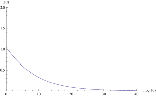
with determined by the beta functions (3.2), with as above. We find that all the couplings run rapidly to zero at high energies, as illustrated in Figure 3.

5.2. Anomalous dimension for the top Yukawa coupling
We have seen above that, at high energies, the coupling constant terms are then subdominant in the running for and for sufficiently large . For the top Yukawa coupling, the analysis of [35] shows that the anomalous dimension satisfies . Thus, one obtains an RGE equation for of the simpler form
| (5.6) |
This can be solved exactly, with solutions that are again of the general form (5.5), this time with parameters
| (5.7) |
Again, the parameter is set to . There is an infrared fixed point with
We analyze the running of the top Yukawa coupling, in the presence of anomalous dimensions, using (5.6) with the assumption, as discussed in [35], that . The initial condition can be taken as in [13], with . We obtain a running where rapidly decays to zero before reaching unification scale. One sees in this way the well known fact that the presence of the gravitational correction terms makes the Yukawa couplings asymptotically free.
5.2.1. Anomalous dimension for the Higgs self-coupling
The qualitative analysis of the running of the Higgs self-coupling given in [35] can be equally applied within the setting of the NCG model. They use an estimate on the anomalous dimension , as suggested in [29], [25]. (We will discuss in §§5.5 and 5.6 some other natural choices of .) The effective action is of the form (4.2), which, as we discussed in §4.2 above is a very good approximation for the spectral action for running between the electroweak and the unification scale. The qualitative analysis of [35] is based on estimating, as above, that the top Yukawa coupling contribution to the beta function for the Higgs self-coupling is dominant over the gauge contribution, which leads to a further simplification of the equation to
| (5.8) |
coupled to the running (5.6) of the top Yukawa . Here again .
The equation (5.8) also gives an approximate fixed point for determined by the equation
| (5.9) |
or equivalently,
| (5.10) |
5.3. Riccati equations and singular linear ODEs
After substituting the explicit general form of the solution for the equation (5.6) for the function , the equation (5.8) for the unknown function becomes a nonlinear ODE of Riccati type,
| (5.11) |
in our case with
| (5.12) |
Riccati equations have the property that they can be transformed into a linear second order ODE by a change of variables of the form
| (5.13) |
This gives a linear equation of the form
| (5.14) |
Using a general form
for the solutions of (5.6), with parameters , , and determined in terms of the coefficients of (5.6) and the initial condition, as discussed above, we obtain a second order linear equation of the form
| (5.15) |
After changing variables to , with , we can write the above as
| (5.16) |
5.4. Polynomial solutions of singular linear ODEs
We consider here special relations between the parameters , , , and that lead to the existence of special polynomial solutions of (5.16).
Following [31], given a linear differential equation of the form
| (5.17) |
where and are functions on some interval of real numbers , one can recursively obtain equations of a similar form for the higher derivatives,
| (5.18) |
where the functions and are recursively defined by
| (5.19) |
Then the equation (5.17) has a polynomial solution of degree at most if and
| (5.20) |
One then has a solution of the form
| (5.21) |
and a general solution of the form
| (5.22) |
The equation (5.16) can be put in the form (5.17) with
| (5.23) |
| (5.24) |
The first step of the recursive equation (5.19) gives
| (5.25) |
| (5.26) |
Thus, at this first step one obtains
The vanishing implies that the parameters should satisfy either and or else and
| (5.27) |
Since both these solutions have they are ruled out for physical reasons. We nonetheless look more closely at the second case. The linear solution in this case is obtained by replacing these values of and in (5.23) and (5.24), so that one gets
A solution is then given by and the general solution by
where
with the latter obtained from the fact that
At the second order, the explicit expressions for and are more involved, but one encounters essentially the same situation. Namely, the condition for the vanishing is given by a system of five equations in the parameters. These equations have solutions
which again are not compatible with having in the solution of the RGE equation for the top Yukawa coupling .
One can see a similar situation for the case of and , where one has several more polynomial solutions, but all of them again under the condition that . In this case one obtains a system of seven equations for the parameters that arise from imposing . The possible solutions to these equations with positive real are the following:
| (5.28) |
Notice how, at least up to degree three, the only condition that is compatible with having a positive anomalous dimension is the relation (5.27) (though not for all values of ).
5.5. Higgs self-coupling and hypergeometric functions
We have seen above that, in the non-physical case with and with the anomalous dimension of the form (5.27), the equation (5.16) admits linear solutions . Here we drop the unphysical condition , but we keep the same constraint on given (5.27), and we show that then the resulting equation (5.16) can be integrated in closed form and has a general solution that can be expressed in terms of hypergeometric functions.
Notice first that, after imposing the condition (5.27), the equation (5.16) can be written in the form (5.17), with
| (5.29) |
We introduce the following auxiliary functions:
| (5.30) |
with
| (5.31) |
and
| (5.32) |
| (5.33) |
We also set
| (5.34) |
| (5.35) |
Then the equation (5.17) with (5.29) has general solution of the form
| (5.36) |
where is the Gauss hypergeometric function.
The corresponding solutions for the original Riccati equation (5.8) that gives the renormalization group flow of the Higgs self coupling are then of the form
| (5.37) |
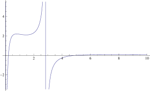
As was already observed in [35], these solutions, for varying choices of the parameters , , , , , can exhibit very complicated and singular behavior (see an example in Figure 5).
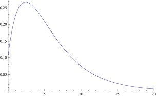
Thus, one needs to ensure the existence of particular solutions that will be compatible with physical assumptions on . So at least one needs a solution for which is positive and does not develop singularities for all . This is, in fact, easy to achieve. For example, setting and , and , with and , gives a solution of the form as in Figure 6.
However, solutions obtained in this way are still not entirely satisfactory from the physical point of view for two main reasons. The first is that we are using the relation (5.27) that expresses as a function of , and . While the example above gives a plausible value of the anomalous dimension , the value considered in (5.7) would give the wrong sign. The other reason is that a solution like the one illustrated in Figure 6, while well behaved in the range , is still plagued by infrared divergences, although these can be pushed very far back in the range.
5.6. Other special solutions of the Higgs self-coupling ODE
The form of the singular linear ODE (5.16) also suggests as a possible natural choice of the value
| (5.38) |
For this value the equation (5.16) simplifies to the form
| (5.39) |
or equivalently to an equation of the form (5.17), with
| (5.40) |
In this case, again, we have an explicit family of solutions in terms of hypergeometric functions. We introduce the following notation.
| (5.41) |
with
| (5.42) |
and as in (5.31) and
| (5.43) |
We then have a general solution of the form
| (5.44) |
with as in (5.35), which is again given in terms of Gauss hypergeometric functions.
One advantage with respect to the family of solutions discussed in the previous section is that now the value of (5.7) is compatible with a positive anomalous dimension . In this case again one can construct examples of solutions for which the resulting function as in (5.37) is continuous and positive for all .
5.7. Implementing a Shaposhnikov–Wetterich-type Higgs mass estimate
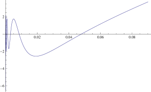
The Higgs mass estimate of 126 GeV derived by Shaposhnikov Wetterich in [35], uses the RGE with anomalous dimensions (5.6) and (5.8), with values of the parameters , with and , , with , where the value is constrained physically by compatibility with the top quark mass. In [35] they use a value of for the anomalous dimension, though they note that their qualitative argument does not depend on the precise values of the anomalous dimensions. Here we work with the explicit solutions in terms of hypergeometric functions, which are instead very sensitive to the explicit values of and . We show here that a slightly larger value of is compatible with the value of used in [35] and with the constraint on imposed by compatibility with the top quark mass. In particular, for GeV, and the Higgs vacuum GeV, which means a value , and keeping the same value of , we obtain .
We have a solution of the equation (5.8) of the form (5.37), with and a solution of (5.16) of the form
| (5.45) |
for
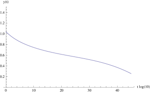
Here the parameter has been assigned the value , while, as above, the parameter is given by , with and the parameter is given by imposing a relation of the form . With the parameters assigned as above, we find that is continuous and positive for all and such that , compatibly with a Higgs mass estimate of , for a slightly larger anomalous dimension . The behavior of this solution for (that is, for ) is illustrated in Figure 8, where we plotted the function

5.8. Infrared behavior
The solutions obtained in this way acquire non-physical negative values, and possibly divergences, at the infrared end of the spectrum. This phenomenon was noticed also in [35] and related to radiatively induced spontaneous symmetry breaking of Coleman–Weinberg type [14]. In fact, the problem with the behavior of solutions for large negative can simply be attributed to the failure, in this range, of the approximations (5.6) and (5.8), where the terms with the coupling constants should be reintroduced as in (3.9) and (3.10), with explicit solutions for the coupling constants of the form (5.5).
6. Geometric conditions at unification
In the models of particle physics based on noncommutative geometry and the spectral action functional, there are several constraints on the parameters at unification energy, imposed by the geometry of the model. We recall here the constraints derived within the model of [13] and we discuss how these are affected by the presence of the gravitational correction terms discussed above in the renormalization group flow.
6.1. Constraints at unification in the CCM model
As discussed in [13] and in §1 of [16], there are constraints on the values of the parameters listed above at unification energy, imposed by the geometry of the model. We recall them here and we refer the reader to the references above for a detailed account of how one obtains these relations. We then show that, in the presence of anomalous dimensions the geometric conditions at unification can be expressed in terms of the presence of a Gaussian matter fixed point for the flow on the moduli space of the finite geometries, and this changes the interpretation of the constraints at unification energy with respect to [13] and [16]. In particular, the Majorana mass terms become compatible with the dark matter models of Shaposhnikov and Tkachev [32], [33], [34], but one loses the geometric see-saw mechanism of [13].
6.1.1. Coupling constants
The normalization of the Yang–Mills terms in the asymptotic expansion of the spectral action ([13]) leads to a unification of the coupling constants with the common value at unification energy satisfying
| (6.1) |
This fixes the value of the parameter of the model in terms of the value at unification of the coupling constants .
6.1.2. Higgs vacuum
The parameter is related to the Higgs vacuum , through the relation
| (6.2) |
which follows from a direct comparison of the terms involving the Yukawa coupling in the asymptotic expansion of the spectral action and in the Lagrangian of the Standard Model (see (4.13) and (4.15) of [13]).
6.1.3. Mass relation
6.1.4. Higgs self-coupling
The value of the Higgs self-coupling parameter at unification energy is predicted to satisfy the relation
| (6.4) |
6.1.5. See-saw mechanism
The see-saw mechanism for the neutrino sector, implemented geometrically by the component of the Dirac operator on acting on the right-handed neutrino sector of the fermion representation, imposes a condition at unification on the parameters , and
| (6.5) |
6.1.6. Gravitational constant
At unification energy the (effective) gravitational constant is related to the parameters , and of the model through
| (6.6) |
6.1.7. Cosmological constant
At unification energy the (effective) gravitational constant is related to the parameters of the model through
| (6.7) |
(We use here the notation for the cosmological constant, as the more commonly used is already taken by the standard notation in NCG for the energy scale in the spectral action.)
6.1.8. Conformal gravity terms
The conformal gravity terms given by the Weyl curvature term and the conformal coupling of the Higgs field to gravity, appear, respectively, with coefficients and . The latter is the standard coefficient for the conformal coupling of the Higgs to gravity. These coefficients are computed after a normalization of the kinetic term of the Higgs.
6.2. The case with anomalous dimensions
When we consider renormalization group equations with gravitational corrections given by anomalous dimensions as in §5, these have a Gaussian matter fixed point at high energies, where the matter fields becomes uncoupled and asymptotically free. This means that the coupling constants and the Yukawa parameters tend rapidly to zero at high energies, as we have seen in the behavior of the solutions to the approximate RGE equations discussed in §5. This leads to a corresponding reinterpretation of the geometric boundary conditions at unification.
In fact, if we interpret the RGE flow as a flow of the finite geometry , the Gaussian matter fixed point corresponds to a fixed point in the moduli space as described in §4.3. This fixed point has trivial coupling constants, and in the fiber over this point of the base it also has trivial Yukawa couplings, so that corresponds to the finite geometry with trivial Dirac operator. Notice that is also a fixed point of all the inner fluctuations of the geometry. Thus, the geometric constraints at unification now become the condition that the finite geometry is close to the fixed point .
In terms of physical consequences of these boundary conditions, one of the primary effects is on the Majorana mass terms. In the setting of [13] the top eigenvalue of the Majorana mass terms matrix is assumed to be near unification scale, so that the three see-saw scales fall in between the unification and the electroweak scale (see a detailed discussion of this point in [22]). This is convenient for a geometric interpretation of the see-saw mechanism for neutrino masses (see [13]). In the setting with anomalous dimensions and Gaussian matter fixed point the behavior of the Majorana mass terms becomes instead consistent with the dark matter models of Shaposhnikov and Tkachev [32], [33], [34], where the Majorana masses are at or below the electroweak scale, thus making them plausible dark matter candidates, in agreement with the exclusion estimates of Kusenko [19].
Comparing with the boundary conditions of [13] recalled above, we see that in the case with Gaussian matter fixed point , the relation (6.4) can be used to fix , while (6.2) fixes the shape of the quartic potential near . The relation (6.5) still fixes , but now no longer implies a see-saw mechanism for neutrino masses, for the reason mentioned above that the Majorana mass scales can fall below the electroweak scale as in the Shaposhnikov–Tkachev models of dark matter [32], [33], [34].
7. Further questions
Some interesting questions arise in connection to the RGE equations discussed in the previous sections. It would be desirable to have a full derivation of Wetterich’s FRGE (4.1), directly expressed in terms of the non-perturbative form of the spectral action, and their compatibility with the RGE flow of [1] for the particle physics sector of the model, with gravitational corrections as in (5.1), (5.2). In view of the recent interest in cosmological applications of the NCG models, it would also be interesting to see how the gravitational corrections to the RGE flow affect the RGE analysis of early universe models of [22] and the constraints on the use of the Higgs as a possible inflation mechanism within this type of models, see [5]. A related question is whether one can obtain constraints on the cosmic topology, via the analysis of [23], [24], and [7], and the effects of the gravitational terms on the running. Other NCG models have been proposed recently, among them the model with supersymmetry of [4] and a model with one lighter and one heavier Higgs [37]. It would be interesting to see what effect the inclusion of gravitational corrections of the form (5.1), (5.2) has on the RGE analysis for these models. In particular, the supersymmetric model of [4], first developed only for the QCD sector, will likely extend to the electroweak sector in a way that is not identical to the MSSM, hence the RGE equations will likely be also different from those of MSSM. The Wetterich method may provide a useful way to perform the RGE analysis of the spectral action for that model.
Acknowledgments
The first author was supported by a Summer Undergraduate Research Fellowship. The second author is partially supported by NSF grants DMS-0901221, DMS-1007207, DMS-1201512, PHY-1205440.
References
- [1] S. Antusch, J. Kersten, M. Lindner, M. Ratz, M.A. Schmidt Running neutrino mass parameters in see-saw scenarios, JHEP 03 (2005) 024, hep-ph/0501272v3.
- [2] H. Arason, D.J. Castano, B. Kesthlyi, E.J. Piard, P. Ramond, B.D. Wright, Renormalization-group study of the standard model and its extensions: the standard model, Phys. Rev. D, 46 (1992) N.9, 3945–3965.
- [3] I.G. Avramidi, Covariant methods for the calculation of the effective action in quantum field theory and investigation of higher- derivative quantum gravity, PhD Thesis, Moscow University, 1986, hep-th/9510140.
- [4] T. van den Broek, W.D. van Suijlekom, Supersymmetric QCD and noncommutative geometry, Comm. Math. Phys. 303 (2011), no. 1, 149–173.
- [5] M. Buck, M. Fairbairn, M. Sakellariadou, Inflation in models with conformally coupled scalar fields: An application to the noncommutative spectral action, Phys. Rev. D 82 (2010) 043509 [14 pages]
- [6] B. Ćaćić, Moduli spaces of Dirac operators for finite spectral triples, in “Quantum groups and noncommutative spaces”, pp. 9–68, Aspects Math., E41, Vieweg Teubner, Wiesbaden, 2011.
- [7] B. Ćaćić, M. Marcolli, K. Teh, Coupling of gravity to matter, spectral action and cosmic topology, arXiv:1106.5473, to appear in Journal of Noncommutative Geometry.
- [8] L. Carminati, B. Iochum, T. Schücker, The noncommutative constraints on the standard model à la Connes, J. Math. Phys. 38 (1997), no. 3, 1269–1280.
- [9] L. Carminati, B. Iochum, D. Kastler, T. Schücker, Relativity, noncommutative geometry, renormalization and particle physics. Coherent states, differential and quantum geometry, Rep. Math. Phys. 43 (1999), no. 1-2, 53–71.
- [10] A. Chamseddine, A. Connes, The spectral action principle, Commun. Math. Phys. 186 (1997) 731–750.
- [11] A. Chamseddine, A. Connes, The uncanny precision of the spectral action, Comm. Math. Phys. 293 (2010), no. 3, 867–897.
- [12] A. Chamseddine, A. Connes, Resilience of the Spectral Standard Model, arXiv:1208.1030.
- [13] A. Chamseddine, A. Connes, M. Marcolli, Gravity and the standard model with neutrino mixing, Adv. Theor. Math. Phys. 11 (2007), no. 6, 991–1089.
- [14] S. Coleman, E. Weinberg, Radiative corrections as the origin of spontaneous symmetry breaking, Phys. Rev. D7 (1973) 1888–1910.
- [15] A. Connes, Gravity coupled with matter and the foundation of noncommutative geometry, Comm. Math. Phys. 182 (1996), no. 1, 155–176.
- [16] A. Connes, M. Marcolli, Noncommutative geometry, quantum fields and motives, Colloquium Publication, Vol.55, American Math. Soc. 2008.
- [17] D. Dou, R. Percacci, The Running Gravitational Couplings, Class. Quant. Grav. 15 (1998) 3449–3468.
- [18] D. Kolodrubetz, M. Marcolli, Boundary conditions of the RGE flow in the noncommutative geometry approach to particle physics and cosmology, Physics Letters B 693 (2010) 166–174.
- [19] A. Kusenko, Sterile neutrinos: the dark side of the light fermions, arXiv:0906.2968.
- [20] O. Lauscher, M. Reuter, Ultraviolet fixed point and generalized flow equation of quantum gravity, Phys. Rev. D 65 (2002) 025013 [44 pages]
- [21] M. Marcolli, Building cosmological models via noncommutative geometry, International Journal of Geometric Methods in Modern Physics, Vol.8, N.5 (2011) 1131–1168.
- [22] M. Marcolli, E. Pierpaoli, Early universe models from noncommutative geometry, Adv. Theor. Math. Phys. 14 (2010), no. 5, 1373–1432.
- [23] M. Marcolli, E. Pierpaoli, K. Teh, The spectral action and cosmic topology, Comm. Math. Phys. 304 (2011), no. 1, 125–174.
- [24] M. Marcolli, E. Pierpaoli, K. Teh, The coupling of topology and inflation in noncommutative cosmology, Comm. Math. Phys. 309 (2012), no. 2, 341–369.
- [25] G. Narain, R. Percacci, Renormalization group flow in scalar-tensor theories, I, arXiv:0911.0386v2.
- [26] W. Nelson, J. Ochoa, M. Sakellariadou, Constraining the noncommutative spectral action via astrophysical observations, Phys. Rev. Lett. 105 (2010) 101602 [5 pages]
- [27] W. Nelson, J. Ochoa, M. Sakellariadou, Gravitational waves in the spectral action of noncommutative geometry, Phys. Rev. D 82 (2010) 085021 [15 pages]
- [28] Y. Okumura, Renormalization group analysis of the Higgs boson mass in a noncommutative differential geometry, Prog. Theor. Phys. 98 (1997) 1333–1344.
- [29] R. Percacci, D. Perini, Asymptotic safety of gravity coupled to matter, hep-th/0304222.
- [30] M. Reuter, Nonperturbative evolution equation for quantum gravity, Phys Rev D 57 (1998) N.2, 971–985.
- [31] N. Saad, R.L. Hall, H. Ciftci, Criterion for polynomial solutions to a class of linear differential equations of second order, J. Phys. A: Math. Gen. 39 (2006) 13445–13454.
- [32] M. Shaposhnikov, The MSM, dark matter and baryon asymmetry of the Universe, Journal of Physics: Conference Series 39 (2006) 9–11.
- [33] M. Shaposhnikov, The MSM, leptonic asymmetries, and properties of singlet fermions, JHEP (2008) 0808:008, 56pp.
- [34] M. Shaposhnikov, I. Tkachev, The MSM, inflation, and dark matter, Phys.Lett. B Vol.639 (2006) 414–417.
- [35] M. Shaposhnikov, C. Wetterich, Asymptotic safety of gravity and the Higgs boson mass, arXiv:0912.0208v2.
- [36] W. Souma, Non-trivial ultraviolet fixed point in quantum gravity, Prog. Theor. Phys. 102 (1999) 181–195.
- [37] C.A. Stephan, New scalar fields in noncommutative geometry, Phys. Rev. D 79 (2009) 065013
- [38] K. Teh, Nonperturbative Spectral Action of Round Coset Spaces of , arXiv:1010.1827, to appear in Journal of Noncommutative Geometry.
- [39] S. Weinberg, Ultraviolet divergences in quantum theories of gravitation, in “General Relativity: an Einstein centenary survey” (S.W. Hawking, W. Israel, Eds.) Cambridge Univ. Press, 1979, pp.790–831.
- [40] C. Wetterich, Exact evolution equation for the effective potential, Phys. Lett. B 301 (1993) 90–94.
- [41] O. Zanusso, L. Zambelli, G.P. Vacca, R. Percacci, Gravitational corrections to Yukawa systems, arXiv:0904.0938v2.