Motivic Brown-Peterson invariants of the rationals

Abstract.

Let $\mathsf{BP}\langle{n}\rangle$, $0\leq n\leq\infty$, denote the family of motivic truncated Brown-Peterson spectra over $\mathbb{Q}$. We employ a “local-to-global” philosophy in order to compute the bigraded homotopy groups of $\mathsf{BP}\langle{n}\rangle$. Along the way, we produce a computation of the homotopy groups of $\mathsf{BP}\langle{n}\rangle$ over $\mathbb{Q}_{2}$, prove a motivic Hasse principle for the spectra $\mathsf{BP}\langle{n}\rangle$, and reprove several classical and recent theorems about the $K$-theory of particular fields in a streamlined fashion. We also compute the bigraded homotopy groups of the 2-complete algebraic cobordism spectrum $\mathsf{MGL}$ over $\mathbb{Q}$.

1. Introduction

In [14], Morel and Voevodsky initated a new approach to studying arithmetic questions by homotopy theoretic means. This involved defining, for any field $k$, an entire homotopy theory called “motivic homotopy theory over $k$.” As part of the apparatus of homotopy theory, one is entitled to a category of objects stabilized by inverting the operation of smashing with a fixed object (such as $S^{1}$, in the classical case). In the motivic case, the most arithmetically interesting choice, of several available, is to localize by inverting smashing with the projective line $\mathbb{P}^{1}$. The outcome of this procedure is Voevodsky’s stable motivic homotopy category, $\mathsf{SH}(k)$ [29]; we call its objects motivic spectra. Many important arithmetic and algebro-geometric cohomology theories are represented by motivic spectra, including motivic cohomology and motivic Steenrod operations, algebraic $K$-theory, and algebraic cobordism. Working in $\mathsf{SH}(k)$ allows us to apply numerous techniques from computational algebraic topology to these invariants. Primary among these examples is the resolution of the Milnor conjecture on Galois cohomology [30]. There has been a recent flurry of concrete computations in stable motivic homotopy theory, led by the efforts of Hu-Kriz-Ormsby, Dugger-Isaksen, and Hill [9, 19, 2, 3].

Each motivic spectrum $\mathsf{E}$ has bigraded homotopy groups

$$\pi_{\star}\mathsf{E}=\bigoplus_{m,n\in\mathbb{Z}}\pi_{m+n\alpha}\mathsf{E}$$

where $\pi_{m+n\alpha}\mathsf{E}$ consists of stable homotopy classes of maps $S^{m+n\alpha}\to\mathsf{E}$. Here $S^{m+n\alpha}=(S^{1})^{\wedge m}\wedge(\mathbb{A}^{1}\smallsetminus 0)^{\wedge n}$.

For judicious choices of $\mathsf{E}$, these bigraded groups carry important information about the base field. For instance, if $\mathsf{E}=\mathsf{KGL}$ is the motivic algebraic $K$-theory spectrum, then $\pi_{m+0\alpha}\mathsf{KGL}=K_{m}(k)$, the $m$-th algebraic $K$-theory group of $k$. If $\mathsf{E}=\mathsf{MGL}$ is the algebraic coboridsm spectrum, then the groups $\pi_{*(1+\alpha)}\mathsf{MGL}=\bigoplus_{k\in\mathbb{Z}}\pi_{k(1+\alpha)}\mathsf{MGL}$ form a ring which corepresents one-dimensional commutative formal groups laws (the Lazard ring).

Let $\mathsf{BP}=\mathsf{BP}_{k}$ denote the motivic Brown-Peterson spectrum at the prime $2$ over a characterstic 0 base field $k$. (N.B. We will often drop the subscript $k$ from our motivic spectrum notation if it is clear that only one field is in play, but we will put the subcript back in whenever the base field needs to be clarified.) The spectrum $\mathsf{BP}$ was constructed by Po Hu and Igor Kriz [7] and Gabriele Vezzosi [28] on the model of Dan Quillen’s idempotent construction in topology [21] and serves as the universal $2$-typical component of $\mathsf{MGL}$. The motivic truncated Brown-Peterson spectra $\mathsf{BP}\langle{n}\rangle=\mathsf{BP}\langle{n}\rangle_{k}$, $0\leq n\leq\infty$, comprise a tower of $\mathsf{BP}$-modules

$$\mathsf{BP}=\mathsf{BP}\langle{\infty}\rangle\rightarrow\cdots\rightarrow\mathsf{BP}\langle{n}\rangle\rightarrow\mathsf{BP}\langle{n-1}\rangle\rightarrow\cdots\rightarrow\mathsf{BP}\langle{0}\rangle.$$

Here, $\mathsf{BP}\langle{0}\rangle=\mathsf{M}\mathbb{Z}_{(2)}$ is the $2$-local motivic Eilenberg-MacLane spectrum by a theorem of Hopkins and Morel, while $\mathsf{BP}\langle{1}\rangle$ is the $2$-local connective $K$-theory spectrum and $\mathsf{BP}$ is the universal $2$-typical algebraically oriented spectrum. (See Lemma 2.9 for the precise way in which $\mathsf{BP}\langle{1}\rangle$ is related to $\mathsf{KGL}$.) As such, for $n>1$ we can view the groups $\pi_{\star}\mathsf{BP}\langle{n}\rangle$ as higher height generalizations of the algebraic $K$-theory of the base field that are constructed from algebraic cobordism.

Our central result is a computation of the bigraded homotopy groups of 2-complete $\mathsf{BP}\langle{n}\rangle$ over the base field $\mathbb{Q}$ via the motivic Adams spectral sequence. The $n=1$ and $n=\infty$ case are of special interest. In the $n=1$ case, we garner a new computation of the 2-complete algebraic $K$-theory of $\mathbb{Q}$ originally arrived at by Rognes and Weibel via the Bloch-Lichtenbaum spectral sequence [23]. Our computation of $\pi_{\star}\mathsf{BP}$ is a first step in a program for computing the motivic stable homotopy groups of the sphere spectrum over $\mathbb{Q}$ via the motivic Adams-Novikov spectral sequence.

In topology, Milnor and Novikov showed independently that complex cobordism splits as a wedge of suspensions of the Brown-Peterson spectrum. Via the motivic Adams spectral sequence, we show in Theorem 2.10 that whenever the $2$-cohomological dimension of $k(\sqrt{-1})$ is finite, $\mathsf{MGL}_{k}$ is the expected wedge of suspensions of $\mathsf{BP}_{k}$’s. (Our condition on $\operatorname{cd}_{2}k(\sqrt{-1})$ ensures that the motivic Adams spectral sequence converges.) As such, Theorem 5.13 also produces a computation of the bigraded coefficients of $\mathsf{MGL}_{\mathbb{Q}}$. This greatly extends the work of Naumann-Spitzweck-Østvær [17] which computes

$$\pi_{m+0\alpha}\mathsf{MGL}\otimes\mathbb{Q}=\begin{cases}\mathbb{Q}&\text{if }m=0\text{ or }m>0\text{ and }4\mid m-1,\\ 0&\text{otherwise}.\end{cases}$$

For the topological $\mathsf{BP}\langle{n}\rangle$ the Adams spectral sequence collapses at the $E_{2}$-page, and its homotopy is

$$\pi_{*}\mathsf{BP}\langle{n}\rangle=\mathbb{Z}_{(2)}[v_{1},\cdots,v_{n}],|v_{i}|=2^{i+1}-2.$$

Over $\mathbb{Q}$ the motivic Adams spectral sequence for $\mathsf{BP}\langle{n}\rangle$ does not collapse at some finite page. We display an elaborate pattern of differentials governed by a Hasse principle in motivic homotopy theory, which is reminiscent of the “local-to-global” methods employed with much success in class field theory and the study of quadratic forms.

Indeed, for each real or $p$-adic completion $\mathbb{Q}_{v}$ of the rationals $\mathbb{Q}$ there is a canonical map

$$\pi_{\star}\mathsf{BP}\langle{n}\rangle_{\mathbb{Q}}\to\pi_{\star}\mathsf{BP}\langle{n}\rangle_{\mathbb{Q}_{v}}$$

to which a map of motivic Adams spectral sequences converges (cf. Proposition 4.6). In Theorem 5.1 we prove that the product of these maps is an injection. The theorem depends on a partial analysis of the motivic Adams spectral sequence for $\mathsf{BP}\langle{n}\rangle_{\mathbb{Q}}$ and then permits a full computation of the spectral sequence (Theorems 5.8 and 5.13).

A more thorough outline of our method is as follows. First, for each real or $p$-adic completion of $\mathbb{Q}$ and for $\mathbb{Q}$ itself, we run a Bockstein spectral sequence which converges to the $E_{2}$-term of the motivic Adams spectral sequence (MASS) for $\mathsf{BP}\langle{n}\rangle$. (These Bockstein spectral sequences are based on filtering the dual Steenrod algebra by powers of $\rho$, the class of $-1$ in Milnor $K$-theory.) We then run the MASS for each real or $p$-adic completion. (These computations are already known for $\mathbb{R}$ and $\mathbb{Q}_{p}$, $p>2$, while our method in this paper is the first to produce a $\mathsf{BP}\langle{n}\rangle$ computation over $\mathbb{Q}_{2}$ for any $n>0$.) Finally, all these computations are combined and analyzed with respect to a global-to-local map that allows us to compute the MASS for $\mathsf{BP}\langle{n}\rangle$ over $\mathbb{Q}$.

Naturally, the results of these computations are quite complicated and are hard to understand without a thorough familiarity with the spectral sequences. We have made a significant effort to present these computations in as digestible a format as possible. The reader can find diagrams for the $\rho$-BSS and MASS for $\mathsf{BP}\langle{3}\rangle_{\mathbb{Q}}$ in Figures 4, 5, and 6. Enough of the patterns present in such computations figure in the $n=3$ case that the reader — with enough diligence and patience — should be able to produce such diagrams for abitrary $n$. The reader is warned that these are not standard spectral sequence charts (homological degree is suppressed and only certain $v_{i}$-multiplications are drawn explicitly) but the graphical calculus is explained in Remarks 3.6 and 5.9.

A closed form for these groups (for arbitrary $n$) is presented in Theorem 5.13 but some qualitative remarks are in order here; we focus on the $m+0\alpha$, $m\geq 2$, component of the bigraded homotopy groups just to give a flavor of the answers (see Section 2 for an explanation of our grading conventions). First, when $m$ is even these groups contain an infinitely generated direct sum of cyclic 2-groups of unbounded order. This summand depends on $m$ but is independent of $n$. Depending on $m$ and $n$, a certain finite number of $\mathbb{Z}/2$ summands may also appear. If $m\equiv 1\pod{4}$, then $\pi_{m}\mathsf{BP}\langle{n}\rangle$ contains a $\mathbb{Z}_{2}$ summand, and this describes all of the non-torsion; an $m,n$-dependent finite number of $\mathbb{Z}/2$ summands may also appear in these degrees. Finally, if $m\equiv 3\pod{4}$ we find an $m,n$-dependent finite $2$-torsion group.

There is a tantalizing connection between the groups calculated in Theorem 5.13 and the standard localization sequence

$$\bigvee_{p}K\mathbb{F}_{p}\to K\mathbb{Z}\to K\mathbb{Q}$$

in algebraic $K$-theory. In fact, in the $n=1$ case our computation naturally splits into components abstractly accounting for the contribution of $\bigvee_{p}K\mathbb{F}_{p}$ and $K\mathbb{Z}$ to $K\mathbb{Q}$. There is a similar abstract splitting for $n>1$ in which case there are no classical localization theorems for $\mathsf{BP}\langle{n}\rangle$ (or associated spectra like motivic $\mathsf{E}(n)$). This leads us to speculate that the motivic spectra $\mathsf{BP}\langle{n}\rangle$, $0\leq n\leq\infty$, should satisfy some sort of localization property (although there are technical details that make the precise statement of such a conjecture nontrivial). We explore these ideas in Remark 5.15; they should provide the basis for continued research on the $\mathsf{BP}\langle{n}\rangle$ spectra.

We now indicate the precise outline of our paper:

In Section 2 we review the motivic Adams spectral sequence (denoted by MASS), the construction of $\mathsf{BP}\langle{n}\rangle$, and the comodule structure of the motivic homology of $\mathsf{BP}\langle{n}\rangle$ over the dual Steenrod algebra. We recall that the MASS converges for $\mathsf{BP}\langle{n}\rangle$ over fields of finite virtual mod-$2$ étale cohomological dimension, a condition which holds for $\mathbb{Q}$ and all of its completions.

In Section 3 we review known MASS computations for $\mathsf{BP}\langle{n}\rangle$ over the real numbers and the $p$-adic rationals, $p>2$, along with a number of applications. We then compute the groups $\pi_{\star}\mathsf{BP}\langle{n}\rangle_{\mathbb{Q}_{2}}$. The usefulness of these computations will be evident in the last part of the paper.

In Section 4 we use base change functors to construct “rational models” for motivic spectra. We apply this to truncated Brown-Peterson spectra. The unit of a base change adjunction allows us to construct the “Hasse map” that compares spectra defined over global and local number fields.

Finally, in Section 5, we combine the Hasse map with the $p$-adic and real MASS computations to prove the Hasse principle for $\mathsf{BP}\langle{n}\rangle$ over $\mathbb{Q}$, and determine its coefficients.

Acknowledgments. Both authors would like to thank Mike Hill for input on this project during the summer of 2009; they would also like to thank Haynes Miller for helpful comments during the preparation of this manuscript.

The first author would like to thank Igor Kriz for initially suggesting that the local-to-global philosophy might be useful in motivic homotopy theory; he also acknowledges partial support from NSF award DMS-1103873.

The second author would like to thank the MIT Mathematics Department for its hospitality and acknowledges partial support from the Leiv Eriksson mobility programme and RCN ES479962.

Finally, both authors would like to thank the referee for timely and constructive comments, and the editors for helpful improvements to the exposition.

2. MASS for $\mathsf{BP}\langle{n}\rangle$

2.1. MASS

For $\mathsf{E}$ a motivic spectrum let $\pi_{\star}\mathsf{E}=\mathsf{E}_{\star}$ denote the bi-graded coefficients

$$\bigoplus_{m,n\in\mathbb{Z}}\pi_{m+n\alpha}\mathsf{E}=\bigoplus_{m,n\in\mathbb{Z}}[S^{m+n\alpha},\mathsf{E}]$$

where $S^{m+n\alpha}=(S^{1})^{\wedge m}\wedge(\mathbb{A}^{1}\smallsetminus 0)^{\wedge n}$.

Let $\mathsf{M}\mathbb{Z}$ be the integral motivic Eilenberg-MacLane spectrum. Its mod-$2$ version $\mathsf{M}\mathbb{Z}/2$ is defined as the smash product of $\mathsf{M}\mathbb{Z}$ with the mod-$2$ motivic Moore spectrum $\mathbf{1}/2$. The bigraded homotopy groups of $\mathsf{M}\mathbb{Z}/2\wedge\mathsf{M}\mathbb{Z}/2$ in the motivic stable homotopy category over any field of characteristic zero identifies with the dual motivic Steenrod algebra [31].

Proposition 2.1.

Over fields of characteristic zero the dual Steenrod algebra $\mathcal{A}_{\star}$ at the prime $2$ is isomorphic to $\mathsf{M}\mathbb{Z}/2_{\star}\mathsf{M}\mathbb{Z}/2$.

We refer to [2, Proposition 7.2] for a short proof of this result, which is based on the identification of Voevodsky’s big category of motives with $\mathsf{M}\mathbb{Z}$-modules [24], [25], and the description of proper Tate motives in [32]. For algebraically closed fields, an alternate proof is given in [9, Theorem 4]. (The proofs in [2] and [9] carry over verbatim to odd primes.)

In the rest of the paper we let $\mathsf{M}$ denote $\mathsf{M}\mathbb{Z}/2$. Let $k^{M}_{*}$ denote the mod 2 Milnor $K$-theory of the base field and recall that $M_{\star}\cong k^{M}_{*}[\tau]$ where $|k^{M}_{n}|=-n\alpha$ and $|\tau|=1-\alpha$.

Next we recall the structure of the dual Steenrod algebra $\mathcal{A}_{\star}$ at $2$ as a Hopf algebroid over the ground ring $\mathsf{M}_{\star}$ [30], [31]. Throughout we use the standard grading convention

$$\mathsf{M}_{\star}=\mathsf{M}^{-\star}.$$

To begin with,

$$\mathcal{A}_{\star}=(\mathsf{M}_{\star},\mathsf{M}_{\star}[\xi_{1},\dots][\tau_{0},\dots]/(\tau_{i}^{2}-\rho(\tau_{i+1}-\tau_{0}\xi_{i+1})-\tau\xi_{i+1})).$$

The left unit in the Hopf algebroid structure is the canonical inclusion, while the right unit is determined by

$$\eta_{R}(\rho)=\rho,\eta_{R}(\tau)=\tau+\rho\tau_{0},$$

for the canonical classes $\tau\in\mathsf{M}_{1-\alpha}\cong\mu_{2}(k)$ and $\rho\in\mathsf{M}_{-\alpha}\cong k^{\times}/(k^{\times})^{2}$. The mod $2$ Bockstein on $\tau$ equals $\rho$. We note that $\mathsf{M}_{\star}\mathsf{M}$ is a commutative free $\mathsf{M}_{\star}$-algebra. Moreover, the polynomial generators have bidegrees

$$|\xi_{i}|=(2^{i}-1)(1+\alpha),\,|\tau_{i}|=1+(2^{i}-1)(1+\alpha),$$

and coproducts given by

$$\Delta\xi_{i}=\sum_{j=0}^{i}\xi_{i-j}^{2^{j}}\otimes\xi_{j},\,\Delta\tau_{i}=\tau_{i}\otimes 1+\sum_{j=0}^{i}\xi_{i-j}^{2^{j}}\otimes\tau_{j}.$$

These are the same formulae as in topology [10], [22, Theorem 3.1.1]. While $\tau$ is not primitive in general, the graded mod-$2$ Milnor $K$-theory ring $k_{\ast}^{M}\subseteq\mathsf{M}_{\star}$ of the base field comprises primitive elements.

Remark 2.2.

Details on the odd-primary dual motivic Steenrod algebra in [31] will not be recounted here since all of our computations occur with $p=2$.

Suppose $\mathsf{E}$ is a motivic homotopy ring spectrum, i.e., a ring object in the motivic stable homotopy category. The homotopy fiber sequence

$$\overline{\mathsf{M}}\rightarrow\mathbf{1}\rightarrow\mathsf{M}$$

gives rise to the Adams resolution

(1)

where

$$\mathsf{E}_{s}=\overline{\mathsf{M}}^{\wedge(s)}\wedge\mathsf{E}.$$

The Künneth isomorphism for motivic cohomology [2, Proposition 7.5] and standard arguments, cf. [2], [9], show that the homotopy spectral sequence associated to (1) is a conditionally convergent spectral sequence

(2) $$E_{2}^{s,m+n\alpha}=\operatorname{Ext}_{\mathcal{A}_{\star}}^{s,m+n\alpha}(\mathsf{M}_{\star},\mathsf{M}_{\star}\mathsf{E})\Longrightarrow\pi_{m-s+n\alpha}\mathsf{E}\,\widehat{}.$$

The target graded group is the motivic homotopy $\pi_{\star}\mathsf{E}\,\widehat{}$ of the nilpotent $\mathsf{M}$-completion of $\mathsf{E}$. This is a tri-graded spectral sequence, where $s$ is the homological degree of the Ext group (the Adams filtration), $m+n\alpha$ is the internal motivic bigrading coming from the bigrading on $\mathcal{A}_{\star}$ and $\mathsf{M}_{\star}$.

The problem of strong convergence of (2) is discussed in [8]. Recall that $\mathsf{E}$ is of finite type if $\mathsf{E}_{m+n\alpha}=0$ for $m\ll 0$. In all of the examples in this paper, the coefficient ring vanishes for $m<0$.

Theorem 2.3.

Suppose $\mathsf{E}$ is cellular and of finite type and $\text{cd}_{2}(k(\sqrt{-1}))<\infty$. Then the $\mathsf{M}$ based Adams spectral sequence (2) is strongly convergent to the homotopy groups of the Bousfield localization of $\mathsf{E}$ at $\mathbf{1}/2$.

Example 2.4.

The assumptions in Theorem 2.3 hold when $k=\mathbb{Q}$, $\mathbb{R}$ and $\mathbb{Q}_{p}$ and $\mathsf{E}$ is one of the following motivic spectra.

• The sphere spectrum $\mathbf{1}$. It follows by results in [13] that $\pi_{m+n\alpha}\mathbf{1}=0$ for $m<0$, cf. [12].

• Algebraic cobordism $\mathsf{MGL}$. We have $\mathsf{MGL}_{m+n\alpha}=0$ for $m<0$ and $\mathsf{MGL}_{-n\alpha}=K_{n}^{M}$ (Milnor $K$-groups of the base field) for $n\geq 0$ [29].

• The algebraic Brown-Peterson spectrum $\mathsf{BP}$. See [7, 28] for constructions. The coefficient ring vanishes for $m<0$ according to the previous example.

• The motivic truncated Brown-Peterson spectra $\mathsf{BP}\langle{n}\rangle$. Again the coefficients vanish for $m<0$ by the previous example.

2.2. $\mathsf{BP}\langle{n}\rangle$

We use the MASS to determine the coefficients of the truncated motivic Brown-Peterson spectra $\mathsf{BP}\langle{n}\rangle$. Here we review the definition and homology of $\mathsf{BP}\langle{n}\rangle$, and specify how we use the latter to compute the $E_{2}$-page of the MASS. We also recall the identifications of $\mathsf{BP}\langle{0}\rangle$ and $\mathsf{BP}\langle{1}\rangle$ in terms of familiar motivic spectra.

Let $\mathsf{BP}=\mathsf{BP}\langle{\infty}\rangle$ denote the motivic Brown-Peterson spectrum constructed from $2$-local algebraic cobordism $\mathsf{MGL}_{(2)}$ via the Quillen idempotent [7, 28]. Inside $\mathsf{MGL}_{(2)\star}$ and $\mathsf{BP}_{\star}$ there are the usual classes $v_{i}$ of degree $(2^{i}-1)(1+\alpha)$. The elements $v_{n+1},v_{n+2},\ldots$ comprise a regular sequence. Following the script in topology, the motivic $\mathsf{BP}\langle{n}\rangle$ is the $\mathsf{BP}$-module formed by killing off the regular sequence $v_{n+1},v_{n+2},\ldots$ in $\mathsf{BP}_{\star}$.

In order to understand the homology of $\mathsf{BP}\langle{n}\rangle$ as a comodule over $\mathcal{A}_{\star}$ we introduce auxiliary Hopf algebroids $\mathcal{E}(n)$ from [3].

Definition 2.5.

Let $\mathcal{E}(n)$ denote the quotient Hopf algebroid

$$\mathcal{E}(n) \mathrel{\mathop{:}}=(\mathsf{M}_{\star},\mathcal{A}/(\xi_{1},\xi_{2},\ldots)+(\tau_{n+1},\tau_{n+2},\ldots))$$

$$=(\mathsf{M}_{\star},\mathsf{M}_{\star}[\tau_{0},\ldots,\tau_{n}]/(\tau_{i}^{2}-\rho\tau_{i+1},\tau_{n}^{2})).$$

We permit $n=\infty$, in which case

$$\mathcal{E}(\infty) \mathrel{\mathop{:}}=(\mathsf{M}_{\star},\mathcal{A}/(\xi_{1},\xi_{2},\ldots))$$

$$=(\mathsf{M}_{\star},\mathsf{M}_{\star}[\tau_{0},\tau_{1},\ldots]/(\tau_{i}^{2}-\rho\tau_{i+1})).$$

In [19], the first author determines the homology of $\mathsf{BP}\langle{n}\rangle$ as a comodule over $\mathcal{A}_{\star}$.

Theorem 2.6.

For $0\leq n\leq\infty$, there is an isomorphism of Hopf algebroids

$$\mathsf{M}_{\star}\mathsf{BP}\langle{n}\rangle=\mathcal{A}\mathbin{\Box}_{\mathcal{E}(n)}\mathsf{M}_{\star}.$$

By change-of-rings we can rewrite the $E_{2}$-term of the MASS for $\mathsf{BP}\langle{n}\rangle$.

Theorem 2.7.

For $0\leq n\leq\infty$, the $E_{2}$-term of the MASS for $\mathsf{BP}\langle{n}\rangle$ is isomorphic to

$$\operatorname{Ext}_{\mathcal{E}(n)}(\mathsf{M}_{\star},\mathsf{M}_{\star}).$$

Theorem 2.7 provides computational control over the $E_{2}$-term of the MASS, and in the next section we will review how the $\rho$-Bockstein spectral sequence produces explicit calculations over particular fields.

Currently, we make precise the connections between $\mathsf{BP}\langle{0}\rangle$ and $\mathsf{BP}\langle{1}\rangle$ and more well-known motivic spectra. These provide motivation for thinking of the $\mathsf{BP}\langle{n}\rangle$, $n\geq 2$, as higher chromatic level spectra in the motivic context (in a sense which we will not make precise in this paper). Throughout our computations we will use the connection between $\mathsf{BP}\langle{0}\rangle$ and $\mathsf{M}\mathbb{Z}$ to initiate calculations, and for each of our $n\geq 1$ results we will comment on the algebraic $K$-theory implications of the $n=1$ case.

The following result follows from announced work of Hopkins and Morel. A detailed proof is given by Hoyois in [4].

Theorem 2.8.

The motivic spectra $\mathsf{BP}\langle{0}\rangle$ and $\mathsf{M}\mathbb{Z}_{(p)}$ are isomorphic over any field of characteristic zero.

The $2$-local connective algebraic $K$-theory spectrum $\mathsf{kgl}_{(2)}$ is precisely $\mathsf{BP}\langle{1}\rangle$ by definition. (At odd primes, $\mathsf{BP}\langle{1}\rangle$ is an Adams summand of localized connective algebraic $K$-theory [15, §4].)

Lemma 2.9.

Suppose $S$ is a separated Noetherian scheme of finite Krull dimension. There exists a connective algebraic $K$-theory motivic spectrum $\mathsf{kgl}$ such that the natural map $\mathsf{kgl}\rightarrow\mathsf{KGL}$ to algebraic $K$-theory becomes a weak equivalence after inverting the Bott map. In particular, if $S=\operatorname{Spec}k$ we have

$$\pi_{m}v_{1}^{-1}\mathsf{BP}\langle{1}\rangle_{k}\cong K_{m}(k)$$

where $K_{*}(k)$ denotes 2-complete algebraic $K$-theory of $k$.

Proof.

Recall that $\mathsf{KGL}$ is the motivic Landweber exact spectrum associated to the $\mathsf{MU}_{\ast}$-algebra

$$x_{1}^{-1}\mathsf{MU}_{\ast}/(x_{2},x_{3},\dots)\mathsf{MU}_{\ast}\cong\mathbb{Z}[x_{1},x_{1}^{-1}]$$

classifying the multiplicative formal group law $\mathsf{x}+\mathsf{y}-x_{1}\mathsf{x}\mathsf{y}$, cf. [16, 17]. Here we employ a fixed isomorphism

$$\mathsf{MU}_{\ast}\cong\mathbb{Z}[x_{1},x_{2},x_{3},\dots]$$

of graded rings where $|x_{i}|=i$ (that is, half of the usual topological grading). The canonical map $\mathsf{MU}_{\ast}\rightarrow\mathsf{MGL}_{*(1+\alpha)}$ affords forming the quotient

$$\mathsf{kgl}=\mathsf{MGL}/(x_{2},x_{3},\dots)$$

by taking iterated cofibers of the multiplication by $x_{i}\in\mathsf{MGL}_{i(1+\alpha)}$ map in the homotopy category of $\mathsf{MGL}$-modules. The orientation map for $\mathsf{KGL}$ sends $x_{i}$ to $0\in\mathsf{KGL}_{i(1+\alpha)}$ for $i\geq 2$. Hence there exists a naturally induced map $\mathsf{kgl}\rightarrow\mathsf{KGL}$. In order to show this map becomes a weak equivalence when inverting the Bott map, i.e.,

$$x_{1}^{-1}\mathsf{kgl}\cong\mathsf{KGL},$$

it suffices, by passing to the colimit, to show that

$$x_{1}^{-1}\mathsf{MGL}/(x_{2},x_{3},\dots,x_{n})$$

is the motivic Landweber exact spectrum associated to the $\mathsf{MU}_{\ast}$-module

$$x_{1}^{-1}\mathsf{MU}_{\ast}/(x_{2},x_{3},\dots,x_{n})$$

for every $n\geq 2$. This can be verified inductively, cf. [26, Theorem 5.2]. ∎

Later, we will use Lemma 2.9 and computations of $\pi_{\star}\mathsf{BP}\langle{1}\rangle$ to prove statements about classical algebraic $K$-theory. One simply inverts $v_{1}$ and reads off the weight 0 component to determine the algebraic $K$-theory of the base field.

We conclude this section by identifying the algebraic cobordism spectrum $\mathsf{MGL}$ with a wedge of suspensions of $\mathsf{BP}$.

Theorem 2.10.

Suppose $k$ is a field with finite virtual cohomological dimension at 2. Let $x_{i}$, $i\geq 1$ denote the standard Lazard ring polynomial generators in degree $i(1+\alpha)$. Let $\mathsf{BP}=\mathsf{BP}_{k}$ and $\mathsf{MGL}=\mathsf{MGL}_{k}$ denote the 2-complete Brown-Peterson and algebraic cobordism spectra over $k$. Let $S$ denote the set of monomials $x_{I}$ in the $x_{i}$ where no factor is of the form $x_{2^{j}-1}$, $j\geq 1$. Then there is an equivalence

(3) $$\bigvee_{x_{I}\in S}\Sigma^{|x_{I}|}\mathsf{BP}\to\mathsf{MGL}.$$

Proof.

The $x_{i}$ exist because $\mathsf{MGL}$ is the universal algebraically oriented spectrum. The maps in (3) are given by multiplication by $x_{I}$. The motivic homology of $\mathsf{BP}$ and $\mathsf{MGL}$ is known by Theorem 2.6 and [1, Proposition 6]. Applying the MASS to (3) we get an isomorphism on $E_{2}$-terms. The MASS converges to homotopy groups of 2-completions because of our hypotheses on $k$ [8]. It follows that (3) is an isomorphism on homotopy groups. Since $\mathsf{MGL}$ and $\mathsf{BP}$ are cellular, we get that (3) is an equivalence. ∎

3. Computations over completions of $\mathbb{Q}$

In this section we review known MASS computations of $\mathsf{BP}\langle{n}\rangle\hat{{}_{2}}_{\star}$ over $\mathbb{C}$, $\mathbb{R}$, and $\mathbb{Q}_{p}$, $p>2$, and present a new calculation of $\mathsf{BP}\langle{n}\rangle\hat{{}_{2}}_{\star}$ over $\mathbb{Q}_{2}$. Here $(~{})\hat{{}_{2}}$ denotes Bousfield localization at the motivic mod 2 Moore spectrum. The differential $d_{r}$ takes the form $E_{r}^{s,m+n\alpha}\rightarrow E_{r}^{s+r,m+r-1+n\alpha}$. When depicting MASS we shall employ “Adams grading” by placing elements of $E_{r}^{s,m+n\alpha}$ in tri-degree $(m-s+n\alpha,s)$, with $\alpha$ along the vertical axis. Thus, in Adams grading, the $r$-th differential has tri-degree $(-1+0\alpha,r)$. The same convention applies to Bockstein spectral sequences.

Notice: In the rest of the paper we elide the 2-completion symbol $(~{})\hat{{}_{2}}$ for legibility. In other words, we proceed to work in the $2$-complete stable motivic homotopy category.

The results over $\mathbb{C}$ are due to Hu-Kriz-Ormsby [9], over $\mathbb{R}$ Mike Hill [3], and over $\mathbb{Q}_{p}$ Ormsby [19]. We recall the differentials here because we will need them in Section 5 to carry out computations over $\mathbb{Q}$.

3.1. The complex place

We begin by discussing the base field $\mathbb{C}$, the complex numbers. These results are not integral to the rest of the paper, but they serve as a nice warm-up case to familiarize the reader with our methods. For $\mathbb{C}$ the motivic Hopf algebra $\mathcal{E}(n)$ (left and right units agree) is the base change of the topological Hopf algebra $\mathcal{E}(n)^{\top}$ to the mod $2$ cohomology ring $\mathbb{F}_{2}[\tau]$ of a point. Here $|\tau|=1-\alpha$. Thus the following result is immediate, cf. [22, Theorem 3.1.16].

Proposition 3.1.

Over $\mathbb{C}$ there is an algebra isomorphism

$$\operatorname{Ext}^{\ast}_{\mathcal{E}(n)}(\mathsf{M}_{\star},\mathsf{M}_{\star})=\mathsf{M}_{\star}[v_{0},\ldots,v_{n}]=\mathbb{F}_{2}[\tau,v_{0},\ldots,v_{n}]$$

where $|\tau|=(1-\alpha,0)$ and $|v_{i}|=((2^{i}-1)(1+\alpha),1)$ in Adams tri-grading.

The generator $v_{i}$ is represented by the class of $\tau_{i}$ in the cobar complex.

Theorem 3.2.

The motivic Adams spectral sequence for $\mathsf{BP}\langle{n}\rangle$ collapses at $E_{2}$ and

$$\mathsf{BP}\langle{n}\rangle_{\star}=(\mathsf{M}\mathbb{Z}_{2})_{\star}[v_{1},\ldots,v_{n}]=\mathbb{Z}_{2}[\tau,v_{1},\ldots,v_{n}]$$

where $|\tau|=1-\alpha,|v_{i}|=(2^{i}-1)(1+\alpha)$. The polynomial generator $v_{1}$ is the Bott periodicity operator for $\mathsf{kgl}=\mathsf{BP}\langle{1}\rangle$.

Proof.

The collapse of the spectral sequence at its $E_{2}$-page follows for tri-degree reasons from Proposition 3.1. The fact that $v_{0}$ detects multiplication by $2$ in $\pi_{0}\mathsf{BP}\langle{n}\rangle=\mathbb{Z}_{2}$ resolves all multiplicative extension problems [3, Lemma 5.4]. ∎

In the $n=1$ case we can deduce an important fact about the algebraic $K$-theory of $\mathbb{C}$ due to Suslin [27].

Lemma 3.3.

Let $\mathcal{E}(n)^{\top}$ denote the variant of $\mathcal{E}(n)$ from topology. The complex topological realization functor induces a map between the Adams spectral sequences for $\mathsf{BP}\langle{n}\rangle_{\mathbb{C}}$

$$\operatorname{Ext}_{\mathcal{E}(n)}^{s,m+n\alpha}(\mathsf{M}_{\star},\mathsf{M}_{\star})\Longrightarrow\pi_{m-s+n\alpha}\mathsf{BP}\langle{n}\rangle_{\mathbb{C}}$$

and the topological $\mathsf{BP}\langle{n}\rangle$ spectrum

$$\operatorname{Ext}_{\mathcal{E}(n)^{\top}}^{s,t}(\mathsf{H}\mathbb{Z}/2_{\ast},\mathsf{H}\mathbb{Z}/2_{\ast})\Longrightarrow\pi_{t-s}\mathsf{BP}\langle{n}\rangle.$$

It sends $\tau$ to $1$ and $v_{i}$ to $v_{i}$ for $i=0,\cdots,n$, and the induced map in weight zero

$$\pi_{m+0\alpha}\mathsf{BP}\langle{n}\rangle_{\mathbb{C}}\rightarrow\pi_{m}\mathsf{BP}\langle{n}\rangle$$

is an isomorphism for all $m\in\mathbb{Z}$.

Remark 3.4.

The isomorphism $K_{\ast}(\mathbb{C})\cong\pi_{\ast}\mathsf{ku}$ was shown by Suslin in [27] using entirely different methods. This is the $n=1$ case of Lemma 3.3. The results in this section generalize to any algebraically closed field of characteristic zero.

3.2. The real place

For the real numbers $\mathbb{R}$, $\mathsf{M}_{\star}=\mathbb{F}_{2}[\tau,\rho]$ as algebras, where $|\tau|=1-\alpha$, $|\rho|=-\alpha$. In order to determine the $\operatorname{Ext}$-groups over $\mathcal{E}(n)$, we can run the $\rho$-Bockstein spectral sequence for $\rho\colon\Sigma^{\alpha}\mathsf{M}\rightarrow\mathsf{M}$. It is an example of the filtration spectral sequence in [22, Theorem A 1.3.9]. This work has been carried out by Hill in [3, Theorem 3.1] who also carefully spells out the properties of the $\rho$-BSS. By comparison with $\mathbb{C}$, the $E_{1}$-term of the $\rho$-BSS takes the form

$$\mathbb{F}_{2}[\tau,\rho,v_{0},\ldots,v_{n}].$$

Proposition 3.5.

Over $\mathbb{R}$, the differentials

$$d_{2^{i+1}-1}\tau^{2^{i}}=\rho^{2^{i+1}-1}v_{i},~{}0\leq i\leq n,$$

determine the $\rho$-Bockstein spectral sequence computing $\operatorname{Ext}_{\mathcal{E}(n)}$.

As an algebra,

$$\operatorname{Ext}^{\star,\ast}_{\mathcal{E}(n)}(\mathsf{M}_{\star},\mathsf{M}_{\star})=\mathbb{F}_{2}[\rho,\tau^{2^{n+1}},v_{i}(j)\mid 0\leq i\leq n,0\leq j]/(\rho^{2^{i+1}-1}v_{i}(j))$$

subject to the additional relations

$$v_{i}(j)v_{k}(\ell)=v_{i}(j+2^{k-i}\ell)v_{k}(0)$$

when $i\leq k$ and

$$v_{i}(j)=\tau^{2^{n+1}}v_{i}(j-2^{n-i})$$

when $j\geq 2^{n-i}$. Here $v_{i}(j)$ is represented on $E_{1}$ by $\tau^{2^{i+1}j}v_{i}$, and has degree

$$(2^{i}(2j+1)-1-(2^{i}(2j-1)+1)\alpha,1)$$

In Section 5 it will be useful to have a thorough understanding of the combinatorics of this spectral sequence. It is difficult to visualize the computation when $n>1$ using standard conventions because the pictures become far too dense. We introduce a graphical calculus below that eliminates this difficulty. We analyze the case of $\mathcal{E}(3)$ in detail.

Remark 3.6.

Figure 1 is a graphical presentation of the spectral sequence in Proposition 3.5 when $n=3$. We have drawn the pictures of this quad-graded spectral sequence in only two dimensions. Recall that each element of the $E_{r}$ page of the $\rho$-BSS has a homological grading $(s,m+n\alpha)$ and also its $\rho$-power filtration. We draw such an element in degree $m-s+n\alpha$ where $m-s$ is plotted on the horizontal axis while $n\alpha$ goes on the vertical axis. As such, these pictures represent the “total Adams degree” of the elements in question. (If they survive the Adams spectral sequence, this is the degree to which they abut.) The authors prefer to think of the degree $s$ as secretly recorded on a third axis coming out of the page, while $\rho$-filtration should be kept track of privately as an extra decoration on each element. In this grading, differentials on the $E_{r}$-page of the $\rho$-BSS point one to the left (with no vertical component) and out of the page one unit as well; they increase the decoration by $\rho$-filtration by $r$.

Note that this is not the “standard” Adams grading, which might draw $m-s+n$ on the horizontal axis and $s$ on the vertical axis, with weight $n\alpha$ and $\rho$-filtration suppressed. We find our pictures more convenient and useful for two reasons. First, weight information is often useful in limiting which differentials are possibly nonzero in $\rho$-Bockstein and motivic Adams spectral sequences. Second, these pictures do a better job of capturing the sort of connectivity that the motivic spectra we study enjoy. In “standard” Adams grading, the copy of mod 2 Milnor $K$-theory in $\mathsf{M}_{\star}$ takes up the entire negative horizontal axis. Since we like to think of $k^{M}_{*}$ as “dimension 0” information in motivic homotopy, it feels better to place it along the vertical axis.

The reader can now interpret the figure via the following key and comments:

$\circ$	$\mathbb{F}_{2}[v_{0},v_{1},v_{2},v_{3}]$
$\bullet$	$\mathbb{F}_{2}[v_{0},v_{1},v_{2},v_{3}]/v_{0}$
$\circledcirc$	$v_{0}\mathbb{F}_{2}[v_{0},v_{1},v_{2},v_{3}]$
$\bullet^{\smallsetminus}$	$\mathbb{F}_{2}[v_{0},v_{1},v_{2},v_{3}]/v_{0},v_{1}$
$\bullet^{\smallsetminus{\kern-3.0pt}\smallsetminus}$	$\mathbb{F}_{2}[v_{0},v_{1},v_{2},v_{3}]/v_{0},v_{1},v_{2}$
$\bullet^{\smallsetminus{\kern-3.0pt}\smallsetminus{\kern-3.0pt}\smallsetminus}$	$\mathbb{F}_{2}[v_{0},v_{1},v_{2},v_{3}]/v_{0},v_{1},v_{2},v_{3}$
$\mid$	$\rho$-multiplication

The authors find it convenient to think of each backslash as “killing off” (or “blocking”) a $v_{i}$-multiplication.

Note, though, that in Figure 1 we do not draw the $v_{i}$-multiplications in the diagram unless a $v_{i}$-multiple is the target of a differential. In general, a copy of $\mathbb{F}_{2}[v_{0},v_{1},v_{2},v_{3}]$ lies in a plane perpendicular to the horizontal and vertical axes which intersects our pictures in a line of slope $1$. (Within this perpendicular plane, $v_{0}$-multiplication is vertical and $v_{i}$-multipliction has slope $1/(2^{i}-1)$.) If a $v_{i}$-multiple is the target of a differential, we draw the appropriate line segment of slope $1$ and draw our differentials hitting these classes; otherwise, $v_{i}$-multiplication is only encoded by our system of circles, dots, and dots with slashes. We do this so that the pictures do not become unmanageably cluttered.

In certain places there are $v_{i}$-multiples, $i>0$, which are divisible by $v_{0}$. This occurs on the classes $v_{0}(j)$ when $j$ is even, and there they are represented by dashed lines of slope 1 (possibly curved to avoid overlap). For example, $v_{1}v_{0}(4)=v_{1}(2)v_{0}$ so there is a dashed line joining $v_{0}(4)$ and $v_{1}(2)$. Similarly, there is a dashed line joining $v_{0}(4)$ and $v_{2}(1)$ because $v_{2}v_{0}(4)=v_{2}(1)v_{0}$.

All labels in these pictures refer to the lowest cohomological degree element in that Adams bi-grading. So while the “target” of the differential on $\tau$ on the $E_{1}$-page is labeled $\rho$, the differential in fact hits $\rho v_{0}$. The necessary number of $v_{0}$’s can be deduced from the cohomological degree of the source and the page number of the spectral sequence.

To extend these pictures to larger $n$, the reader simply needs to reinterpret $\circ$ as $\mathbb{F}_{2}[v_{0},\ldots,v_{n}]$ and $\bullet$ with $k$ slashes as $\mathbb{F}_{2}[v_{0},\ldots,v_{n}]/v_{0},\ldots,v_{k}$. If $n>3$, then $\tau^{16}$ will support a differential and there will be a yet more elaborate pattern on $\tau^{16}$ in the $E_{\infty}$ page. Similar statements hold for $\tau^{32},\tau^{64}$, etc.

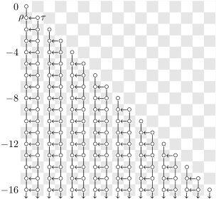
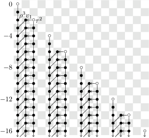
$E_{1}$		$E_{3}$

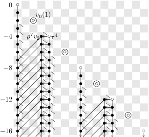
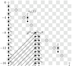
$E_{7}$		$E_{15}$

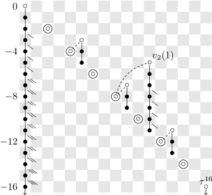
$E_{\infty}$

Figure 1. The $\rho$-BSS for $\operatorname{Ext}_{\mathcal{E}(3)}$ over $\mathbb{R}$.

Recall from [3, Theorem 5.3, Corollary 5.7] the collapse of the MASS for $\mathsf{BP}\langle{n}\rangle$ over $\mathbb{R}$. Combined with the Real truncated Brown-Peterson spectra computations due to Hu in [6], appropriately amended, we arrive at the following result.

Theorem 3.7.

The motivic Adams spectral sequence for $\mathsf{BP}\langle{n}\rangle$ over $\mathbb{R}$ collapses at $E_{2}$ and the homotopy $\mathsf{BP}\langle{n}\rangle_{\star}$ is given additively by

$$\mathbb{Z}_{2}[\rho,\tau^{2^{n+1}},v_{i}(j)\mid 0\leq i\leq n,0\leq j]$$

subject to the relations $v_{0}(0)=2$, $\rho^{2^{i+1}-1}v_{i}(j)$, $v_{i}(j)v_{k}(\ell)=v_{i}(j+2^{k-i}\ell)v_{k}(0)$ when $i\leq k$, and $v_{i}(j)=\tau^{2^{n+1}}v_{i}(j-2^{n-i})$ when $j\geq 2^{n-i}$. The degree of $v_{i}(j)$ is $(2^{i}-1)(1+\alpha)+2^{i+1}j(1-\alpha)$. (If $n=\infty$ one should read the expression as lacking a $\tau$-power generator and having $v_{i}(j)$ generators for $0\leq i<\infty,~{}0\leq j$.)

Remark 3.8.

While his methods are quite different, it should also be noted that Nobuaki Yagita produced similar computations for the homotopy of $\mathsf{BP}/2$ over $\mathbb{R}$ via the Atiyah-Hirzebruch spectral sequence, cf. [33].

For the inclusion $i\colon\mathbb{R}\subset\mathbb{C}$ recall the identity map on $\mathsf{BP}\langle{n}\rangle_{\mathbb{C}}$ induces a comparison map

$$\mathsf{BP}\langle{n}\rangle_{\mathbb{R}}\to i_{\ast}\mathsf{BP}\langle{n}\rangle_{\mathbb{C}}.$$

(See Section 4 if the above technology is unfamiliar.) Applying the complex topological realization functor to $\mathsf{BP}\langle{n}\rangle_{\mathbb{R}}$ yields the comparison with the topological truncated Brown-Peterson spectrum $\mathsf{BP}\langle{n}\rangle$.

On homotopy groups, see also Proposition 4.3, the first comparison map is determined by the following result.

Lemma 3.9.

The comparison map for $i\colon\mathbb{R}\subset\mathbb{C}$ induces a map between the motivic Adams spectral sequences for $\mathsf{BP}\langle{n}\rangle_{\mathbb{R}}$

$$\operatorname{Ext}_{\mathcal{E}(n)}^{s,m+n\alpha}(\mathsf{M}_{\ast},\mathsf{M}_{\ast})\Longrightarrow\pi_{m-s+n\alpha}\mathsf{BP}\langle{n}\rangle_{\mathbb{R}}$$

and for $\mathsf{BP}\langle{n}\rangle_{\mathbb{C}}$

$$\operatorname{Ext}_{\mathcal{E}(n)}^{s,m+n\alpha}(\mathsf{M}_{\ast},\mathsf{M}_{\ast})\Longrightarrow\pi_{m-s+n\alpha}\mathsf{BP}\langle{n}\rangle_{\mathbb{C}}.$$

It sends $\rho$ to $0$, $\tau^{2^{n+1}}$ to $\tau^{2^{n+1}}$, and $v_{i}(j)$ to $\tau^{2^{i+1}j}v_{i}$ for $0\leq i\leq n$.

Remark 3.10.

Comparing $v_{0}$-towers for the spectral sequences in Lemma 3.9 implies the map $K_{m}(\mathbb{R})\to K_{m}(\mathbb{C})$ is an isomorphism when $m\equiv 0\bmod 8$, the multiplication by $2$ map on $\mathbb{Z}_{2}$ when $m\equiv 4\bmod 8$ and trivial otherwise.

Lemma 3.11.

The complex topological realization functor induces a map between the motivic Adams spectral sequences for $\mathsf{BP}\langle{n}\rangle_{\mathbb{R}}$

$$\operatorname{Ext}_{\mathcal{E}(n)}^{s,m+n\alpha}(\mathsf{M}_{\ast},\mathsf{M}_{\ast})\Longrightarrow\pi_{m-s+n\alpha}\mathsf{BP}\langle{n}\rangle_{\mathbb{R}}$$

and the topological $\mathsf{BP}\langle{n}\rangle$ spectrum

$$\operatorname{Ext}_{\mathcal{E}(n)^{\top}}^{s,t}(\mathsf{H}\mathbb{Z}/2_{\ast},\mathsf{H}\mathbb{Z}/2_{\ast})\Longrightarrow\pi_{t-s}\mathsf{BP}\langle{n}\rangle.$$

It sends $\rho$ to $0$, $\tau^{2^{n+1}}$ to $1$, and $v_{i}(j)$ to $v_{i}$ for $0\leq i\leq n$.

Remark 3.12.

The real topological realization functor takes $\mathsf{kgl}_{\mathbb{R}}$ to a trivial spectrum.

We can identify the weight zero subalgebra of $\pi_{\star}\mathsf{BP}\langle{1}\rangle_{\mathbb{R}}$ with the coefficient ring of $2$-completed connective real topological $K$-theory.

Lemma 3.13.

The subalgebra $\pi_{\ast+0\alpha}\mathsf{BP}\langle{1}\rangle_{\mathbb{R}}$ is isomorphic to $\pi_{\ast}\mathsf{ko}$.

Proof.

Recall the ring isomorphism

$$\pi_{\ast}\mathsf{ko}\cong\mathbb{Z}_{2}[\eta,\alpha,\beta]/(2\eta,\eta^{3},\eta\alpha,\alpha^{2}-4\beta),$$

where $|\eta|=1$, $|\alpha|=4$ and $|\beta|=8$, cf. [22, Theorem 3.1.26]. We have

$$\pi_{\star}\mathsf{BP}\langle{1}\rangle_{\mathbb{R}}=\mathbb{Z}_{2}[\rho,\tau^{4},v_{0}(1),v_{1}]/(2\rho,\rho^{3}v_{1},v_{0}(1)^{2}-4\tau^{4}).$$

The assertion follows by mapping $\pi_{\ast}\mathsf{ko}$ into $\pi_{\star}\mathsf{BP}\langle{1}\rangle_{\mathbb{R}}$ by sending $\eta$ to $\rho v_{1}$, $\alpha$ to $v_{0}(1)v_{1}^{2}$ and $\beta$ to $\tau^{4}v_{1}^{4}$. ∎

Remark 3.14.

The isomorphism $K_{\ast}(\mathbb{R})\cong\pi_{\ast}\mathsf{ko}$ was shown by Suslin in [27] using entirely different methods. The results in this section generalizes to all real closed fields, e.g., the field $\overline{\mathbb{Q}}\cap\mathbb{R}$ of real algebraic numbers.

Remark 3.15.

Following the reasoning after the proof of Lemma 5.4 in [3], we can explain Lemma 3.13 by considering the realification functor $t$ from $\mathbb{P}^{1}$-spectra over $\mathbb{R}$ to $\mathbb{Z}/2$-equivariant spectra. It should be the case that $t(\mathsf{BP}\langle{n}\rangle_{\mathbb{R}})=\mathsf{BP}\mathbb{R}\langle n\rangle$, where the spectrum $\mathsf{BP}\mathbb{R}\langle n\rangle$ is the Real truncated Brown-Peterson spectrum of Po Hu [6]. This then induces a map

$$\pi_{*+0\alpha}\mathsf{BP}\langle{n}\rangle_{\mathbb{R}}\to\pi_{*+0\sigma}\mathsf{BP}\mathbb{R}\langle n\rangle$$

where $\sigma$ is the sign representation of $\mathbb{Z}/2$ and we are working with $RO(\mathbb{Z}/2)$-graded homotopy groups. Now the target of this map is easily identified with $\pi_{*}\mathsf{BP}\mathbb{R}\langle n\rangle^{\mathbb{Z}/2}$ and Hu shows in [6] that $\mathsf{BP}\mathbb{R}\langle 1\rangle^{\mathbb{Z}/2}\simeq\mathsf{ko}$. Hence the above map induces the isomorphism of Lemma 3.13

3.3. Non-Archimedean places

Let $p$ be an odd prime number. In [19], the first author determines the behavior of the $\rho$-Bockstein and motivic Adams spectral sequences for $\mathsf{BP}\langle{n}\rangle$ over $\mathbb{Q}_{p}$. The differentials observed are quite similar to those for $\mathsf{BP}\langle{n}\rangle$ over $\mathbb{R}$, but the $\rho$-BSS always collapses at $E_{2}$ and there are (infinitely many) nontrivial differentials in the MASS.

Recall that

$$k^{M}_{*}(\mathbb{Q}_{p})=\begin{cases}\mathbb{F}_{2}[u,p]/(u^{2},p^{2})&\text{if }p\equiv 1\pod{4},\\ \mathbb{F}_{2}[u,p]/(u^{2},p(u-p))&\text{if }p\equiv 3\pod{4},\end{cases}$$

where $u$ is a nonsquare in the Teichmüller lift $\mathbb{F}_{p}^{\times}\subset\mathbb{Q}_{p}^{\times}$, and $p$ is the class of the uniformizer $p$. If $p\equiv 3\pod{4}$ we choose $u$ to be the class of $\rho$, the class of $-1$, while $\rho=0$ when $p\equiv 1\pod{4}$. Recall that $\mathsf{M}_{\star}=k^{M}_{*}[\tau]$.

The following is the main result of [19, §4].

Theorem 3.16.

If $p\equiv 1\pod{4}$ then the $\rho$-BSS for $\operatorname{Ext}_{\mathcal{E}(n)}$ over $\mathbb{Q}_{p}$ collapses and

$$\operatorname{Ext}_{\mathcal{E}(n)}(\mathsf{M}_{\star},\mathsf{M}_{\star})=\mathsf{M}_{\star}[v_{0},\ldots,v_{n}].$$

If $p\equiv 3\pod{4}$ then the $\rho$-BSS for $\operatorname{Ext}_{\mathcal{E}(n)}$ is determined by the differential

$$d_{1}\tau=\rho v_{0}$$

and

$$\operatorname{Ext}_{\mathcal{E}(n)}(\mathsf{M}_{\star},\mathsf{M}_{\star})=k^{M}_{*}[\tau^{2},v_{0},\ldots,v_{n}]/\rho v_{0}\oplus\rho\tau k^{M}_{*}[\tau^{2},v_{0},\ldots,v_{n}].$$

Let $\varepsilon(p)=\nu_{2}(p-1)$ and $\lambda(p)=\nu_{2}(p^{2}-1)$ where $\nu_{2}$ is the 2-adic valuation. Then [19, §5] shows that the MASS for $\mathsf{BP}\langle{n}\rangle$ over $\mathbb{Q}_{p}$ takes the following form.

Theorem 3.17.

If $p\equiv 1\pod{4}$, then the MASS for $\mathsf{BP}\langle{n}\rangle$ over $\mathbb{Q}_{p}$ is determined by differentials

$$d_{\varepsilon(p)+i}\tau^{2^{i}}=u\tau^{2^{i}-1}v_{0}^{\varepsilon(p)+i}.$$

If $p\equiv 3\pod{4}$, then the MASS for $\mathsf{BP}\langle{n}\rangle$ over $\mathbb{Q}_{p}$ is determined by

$$d_{\lambda(p)-1+i}\tau^{2^{i}}=\rho\tau^{2^{i}-1}v_{0}^{\lambda(p)-1+i}.$$

For a description of the $E_{\infty}$ term see [19, Theorem 5.7].

Set $k=\varepsilon(p)$ if $p\equiv 1\pod{4}$ and set $k=\lambda(p)$ if $p\equiv 3\pod{4}$. The MASS for $\mathsf{BP}\langle{n}\rangle$ over $\mathbb{Q}_{p}$ is depicted graphically in Figure 2 using the same conventions as Figure 1 (see Remark 3.6) with the addition that $\circ/v_{0}^{r}=\mathbb{F}_{2}[v_{0},\ldots,v_{n}]/v_{0}^{r}$ and that Adams spectral sequences no longer have a $\rho$-filtration grading. (That said, the $E_{k}$ page is actually the $\rho$-BSS if $k=1$.)

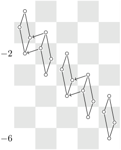
$E_{k}$	$E_{k+1}$
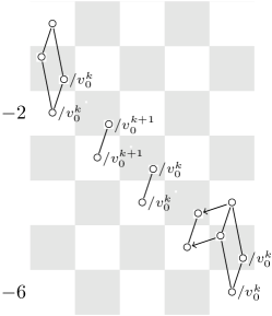
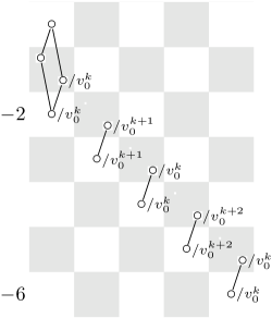
$E_{k+2}$	$E_{k+3}$

Figure 2. The MASS for $\mathsf{BP}\langle{n}\rangle$ over $\mathbb{Q}_{p}$, $p>2$.

We now turn our attention to the field $\mathbb{Q}_{2}$. The first mod 2 Milnor $K$-theory of $\mathbb{Q}_{2}$ is generated by the classes of $-1$, $2$, and $5$, which we denote $\rho$, $x$, and $y$, respectively. Then

$$k^{M}_{*}(\mathbb{Q}_{2})=\mathbb{F}_{2}[\rho,x,y]/(\rho^{3},x^{2},y^{2},\rho^{2}+xy,\rho x,\rho y).$$

Theorem 3.18.

The $\rho$-BSS for $\operatorname{Ext}_{\mathcal{E}(n)}$ over $\mathbb{Q}_{2}$ is determined by the differential

$$d_{1}\tau=\rho v_{0}.$$

Proof.

We compute $d_{1}\tau$ as $\eta_{L}(\tau)-\eta_{R}(\tau)=\rho v_{0}$. Further differentials follow the pattern of Proposition 3.5, but $\rho^{3}=0$ in $k^{M}_{*}(\mathbb{Q}_{2})$ so the spectral sequence collapses at $E_{2}$. ∎

Theorem 3.19.

The MASS for $\mathsf{BP}\langle{n}\rangle$ over $\mathbb{Q}_{2}$ is determined by the differentials

$$d_{2+i}\tau^{2^{i}}=x\tau^{2^{i}-1}v_{0}^{2+i}$$

for $1\leq i$.

Proof.

We first treat the case $n=0$ in which we utilize a comparison with étale cohomology. Applying the universal coefficient theorem and results in [18, Chapter VII] yields

$$(\mathsf{M}\mathbb{Z}_{2})_{m+n\alpha}=\begin{cases}\mathbb{Z}_{2}&\text{if }m=n=0,\\ \mathbb{Z}_{2}^{\oplus 2}\oplus\mathbb{Z}/2&\text{if }m=0,n=-1,\\ \mathbb{Z}/2&\text{if }m=0,n=-2,\\ \mathbb{Z}_{2}\oplus\mathbb{Z}/2&\text{if }n=-(m+1)<-1,~{}m\text{ even},\\ \mathbb{Z}_{2}\oplus\mathbb{Z}/2^{2+\nu_{2}(m+1)}&\text{if }n=-(m+1)<-1,~{}m\text{ odd},\\ \mathbb{Z}/2&\text{if }n=-(m+2)<-2,~{}m\text{ even},\\ \mathbb{Z}/2^{2+\nu_{2}(m+1)}&\text{if }n=-(m+2)<-2,~{}m\text{ odd},\\ 0&\text{otherwise}.\end{cases}$$

In order to have the correct 2-torsion in degrees of the form $m-(m+1)\alpha$ we must have $d_{2+i}\tau^{2^{i}}=z\tau^{2^{i}-1}v_{0}^{2+i}$ for $z$ a nonzero linear combination of $x$ and $y$. In Lemma 5.7 we show that $z=x$. (The proof is deferred because it relies on the Hasse map defined in the next section.)

For $n>0$ consider the linearization map $\mathsf{BP}\langle{n}\rangle\to\mathsf{BP}\langle{0}\rangle$ and the induced map of spectral sequences. By tri-degree considerations we can identify the spectral sequence for $\mathsf{BP}\langle{n}\rangle$ as $E_{*}(\mathsf{BP}\langle{0}\rangle)[v_{1},\ldots,v_{n}]$ where the $v_{>0}$ are permanent cycles. This concludes the proof. ∎

The behavior of the spectral sequence is pictured in Figure 3 using the same conventions as Figure 2. In the dimensional range pictured $E_{5}=E_{\infty}$.

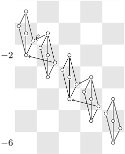
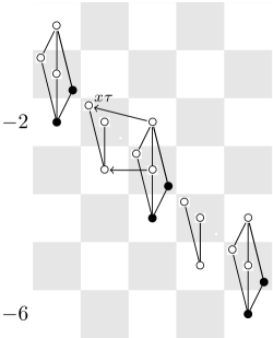
$E_{1}$	$E_{3}$
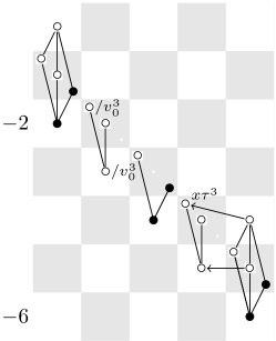
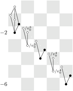
$E_{4}$	$E_{5}$

Figure 3. The $\rho$-BSS and MASS for $\mathsf{BP}\langle{n}\rangle$ over $\mathbb{Q}_{2}$

Corollary 3.20.

Over $\mathbb{Q}_{2}$ we have $\mathsf{BP}\langle{n}\rangle_{\star}=(\mathsf{M}\mathbb{Z}_{2})_{\star}[v_{1},\cdots,v_{n}]$.

4. The Hasse map

Our goal now is to use the local data from the previous section to produce global computations. To this end, we need a method for comparing the local and global variants of $\mathsf{BP}\langle{n}\rangle$. In this section we construct a Hasse map which serves this purpose.

For any scheme map $f:S\to T$ there is a base change functor

$$f^{*}:\operatorname{Sp}(T)\to\operatorname{Sp}(S)$$

from $T$-spectra to $S$-spectra admitting a right adjoint

$$f_{*}:\operatorname{Sp}(S)\to\operatorname{Sp}(T).$$

Let $\mathsf{BP}\langle{n}\rangle_{S}$ denote the truncated Brown-Peterson spectrum in $S$-spectra. Recall that $\mathsf{BP}\langle{n}\rangle_{S}$ is constructed from $\mathsf{MGL}_{S}$ by $p$-localizing, taking the iterated colimit of the Quillen idempotent (producing $\mathsf{BP}_{S}$) and then killing off $v_{i}$, $i>n$. Recall the isomorphism $\mathsf{MGL}_{S}\cong f^{*}\mathsf{MGL}_{T}$ for $f$ as above.

Proposition 4.1.

The truncated Brown-Peterson spectra $\mathsf{BP}\langle{n}\rangle$ satisfy

$$\mathsf{BP}\langle{n}\rangle_{S}\cong f^{*}\mathsf{BP}\langle{n}\rangle_{T}.$$

Proof.

Localization at $p$, inverting the Quillen idempotent, and killing $v_{i}$’s are all colimit constructions; $f^{*}$ commutes with colimits because it is a left adjoint. ∎

For $v$ a real or $p$-adic place of $\mathbb{Q}$ we denote by $i_{v}:\operatorname{Spec}\mathbb{Q}_{v}\to\operatorname{Spec}\mathbb{Q}$ the map of Zariski spectra induced by the field extension $\mathbb{Q}_{v}/\mathbb{Q}$.

Consider a family of motivic spectra (over different base fields) $\mathsf{E}=\{\mathsf{E}_{k}=\mathsf{E}_{\operatorname{Spec}k}\in\mathsf{SH}(k)\mid k=\mathbb{Q}\text{ or }\mathbb{Q}_{v}\}$. In the following we assume that this family satisfies $\mathsf{E}_{\mathbb{Q}_{v}}\cong i_{v}^{*}\mathsf{E}_{\mathbb{Q}}$ for all non-complex places $v$ of $\mathbb{Q}$.

Definition 4.2.

The rational model of $\mathsf{E}_{\mathbb{Q}_{v}}$ is defined as

$$\mathsf{E}^{\mathbb{Q}}_{\mathbb{Q}_{v}}\mathrel{\mathop{:}}=i_{v}{}_{*}\mathsf{E}_{\mathbb{Q}_{v}}\cong i_{v}{}_{*}i_{v}^{*}\mathsf{E}_{\mathbb{Q}}.$$

The terminology is justified by the following proposition.

Proposition 4.3.

The bigraded homotopy groups of $\mathsf{E}^{\mathbb{Q}}_{\mathbb{Q}_{v}}$ (computed in $\mathsf{SH}(\mathbb{Q})$, the stable motivic homotopy category over $\mathbb{Q}$) are isomorphic to those of $\mathsf{E}_{\mathbb{Q}_{v}}$ in $\mathsf{SH}(\mathbb{Q}_{v})$.

Proof.

By adjunction isomorphisms and the fact that $i_{v}^{*}\mathbf{1}_{\mathbb{Q}}=\mathbf{1}_{\mathbb{Q}_{v}}$ we have

$$\pi_{\star}^{\mathbb{Q}}\mathsf{E}^{\mathbb{Q}}_{\mathbb{Q}_{v}}=[\mathbf{1}_{\mathbb{Q}},\mathsf{E}^{\mathbb{Q}}_{\mathbb{Q}_{v}}]^{\mathbb{Q}}_{\star}=[\mathbf{1}_{\mathbb{Q}},i_{v}{}_{*}\mathsf{E}_{\mathbb{Q}_{v}}]^{\mathbb{Q}}_{\star}=[i_{v}^{*}\mathbf{1}_{\mathbb{Q}},\mathsf{E}_{\mathbb{Q}_{v}}]^{\mathbb{Q}_{v}}_{\star}=[\mathbf{1}_{\mathbb{Q}_{v}},\mathsf{E}_{\mathbb{Q}_{v}}]^{\mathbb{Q}_{v}}_{\star}.$$

This is by definition the homotopy groups $\pi_{\star}^{\mathbb{Q}_{v}}\mathsf{E}_{\mathbb{Q}_{v}}$ of $\mathsf{E}_{\mathbb{Q}_{v}}$ in $\mathsf{SH}(\mathbb{Q}_{v})$. ∎

Since $\mathsf{E}^{\mathbb{Q}}_{\mathbb{Q}_{v}}\cong i_{v}{}_{*}i_{v}^{*}\mathsf{E}_{\mathbb{Q}}$ the $(i_{v}^{*},i_{v}{}_{*})$ adjunction unit induces a map

$$\eta_{v}:\mathsf{E}_{\mathbb{Q}}\to\mathsf{E}_{\mathbb{Q}_{v}}^{\mathbb{Q}}.$$

Definition 4.4.

For $\mathsf{E}$ as above, the motivic Hasse map is given by

$$H_{\mathsf{E}}\mathrel{\mathop{:}}=\prod\pi_{\star}\eta_{v}:\pi_{\star}\mathsf{E}_{\mathbb{Q}}\to\prod\pi_{\star}\mathsf{E}_{\mathbb{Q}_{v}}^{\mathbb{Q}}$$

where the product runs over real and $p$-adic places $v$.

Definition 4.5.

The family of spectra $\mathsf{E}$ satisfies the motivic Hasse principle if the motivic Hasse map $H_{\mathsf{E}}$ is monic.

Proposition 4.6.

The Hasse map takes the form

$$H_{\mathsf{E}}:\pi_{\star}^{\mathbb{Q}}\mathsf{E}_{\mathbb{Q}}\to\prod\pi_{\star}^{\mathbb{Q}_{v}}\mathsf{E}_{\mathbb{Q}_{v}}.$$

Proof.

This is a consequence of Proposition 4.3. Note that the target cannot be pared down to a direct sum. For instance, if we take $\mathsf{E}=\mathbf{1}$ we find that $\rho$ has nontrivial image in infinitely many of the groups $\pi_{-\alpha}^{\mathbb{Q}_{v}}\mathbf{1}_{\mathbb{Q}_{v}}$. ∎

The Hasse maps of interest in this paper are the ones for $\mathsf{BP}\langle{n}\rangle$, $0\leq n\leq\infty$. Let $E_{*}^{*,\star}(k)$ denote the MASS for $\mathsf{BP}\langle{n}\rangle_{k}$. Then the Hasse map induces a map of MASSs

(4) $$E_{*}^{*,\star}(\mathbb{Q})\to\prod_{v}E_{*}^{*,\star}(\mathbb{Q}_{v}).$$

5. Computations over $\mathbb{Q}$ and the motivic Hasse principle

This section proves the main theorem of this paper.

Theorem 5.1.

The truncated Brown-Peterson spectra $\mathsf{BP}\langle{n}\rangle$ satisfy the motivic Hasse principle.

Corollary 5.2.

There are no hidden multiplicative extensions in the motivic Adams spectral sequence for $\mathsf{BP}\langle{n}\rangle$ over $\mathbb{Q}$ and $v_{0}$-multiplication represents multiplication by 2.

Proof.

The computations with local fields in Section 3 show the result holds for all completions of $\mathbb{Q}$. Thus our claim follows from Theorem 5.1. (Note that, in general, $v_{0}=2+\rho\eta$, but $\eta=0$ in $\pi_{\alpha}\mathsf{BP}\langle{n}\rangle$.) ∎

Our proof of Theorem 5.1 follows from an analysis of (4). Carrying that analysis a few steps further we also get a computation of $\pi_{\star}\mathsf{BP}\langle{n}\rangle$ over $\mathbb{Q}$, $0\leq n\leq\infty$, which is stated in Theorem 5.8 below.

To get these computations off the ground we need a detailed understanding of $k^{M}_{*}(\mathbb{Q})$ and the Hasse map

$$k^{M}_{*}(\mathbb{Q})\to\prod_{v}k^{M}_{*}(\mathbb{Q}_{v}).$$

The following proposition consists of basic facts easily deduced from, e.g., [11, Example 1.8 and Appendix].

Proposition 5.3.

The mod 2 Milnor K-theory of $\mathbb{Q}$ has the following structure:

$$k^{M}_{0}(\mathbb{Q}) =\mathbb{Z}/2,$$

$$k^{M}_{1}(\mathbb{Q}) =\mathbb{Z}/2\{\rho\}\oplus\bigoplus_{p\geq 2}\mathbb{Z}/2\{[p]\},$$

$$k^{M}_{2}(\mathbb{Q}) =\mathbb{Z}/2\{\rho^{2}\}\oplus\bigoplus_{p\geq 3}\mathbb{Z}/2\{a_{p}\},$$

$$k^{M}_{n}(\mathbb{Q}) =\mathbb{Z}/2\{\rho^{n}\}\text{ if }n\geq 3.$$

Multiplication follows the rule

$$[\ell]\cdot[q]=(\ell,q)_{2}\rho^{2}+\sum_{p\geq 3}(\ell,q)_{p}a_{p}$$

where $\ell$ and $q$ are primes or $-1$, $(~{},~{})_{p}$ is the Hilbert symbol if $p\geq 3$, and $(~{},~{})_{2}$ is the 2-adic Steinberg symbol.

The Hasse map takes pure symbols to their obvious images in $\prod k^{M}_{1}(\mathbb{Q}_{v})$ and takes $a_{p}$ to the unique nonzero class in $k^{M}_{2}(\mathbb{Q}_{p})$ and to $0$ in $k^{M}_{2}(\mathbb{Q}_{\ell})$, $\ell\neq p$.

It will be convenient to understand the $\rho$-module structure of $k^{M}_{*}(\mathbb{Q})$.

Proposition 5.4.

The $\rho$-module structure of $k^{M}_{*}(\mathbb{Q})$ is such that $\rho$ is not nilpotent and

$$\rho\cdot[p] =0\text{ if }p\equiv 1\pod{4},$$

$$\rho\cdot[p] =\rho^{2}+a_{p}\text{ if }p\equiv 3\pod{4},$$

$$\rho\cdot[2] =0.$$

Proof.

The class $\rho$ is non-nilpotent because $\mathbb{Q}$ has a real embedding. (Note that Propositions 5.3 and 5.4 omit a few multiplicative relations in $k^{M}_{*}(\mathbb{Q})$ that are not important in any of our calculations.)

The relations follow from computations of Hilbert and 2-adic Steinberg symbols. Recall that for $a=2^{\alpha}u$, $b=2^{\beta}v$ for $u,v$ odd we have

$$(a,b)_{2}=(-1)^{\frac{u-1}{2}\frac{v-1}{2}+\alpha\frac{v^{2}-1}{8}+\beta\frac{u^{2}-1}{8}}.$$

Hence

$$(-1,p)_{2}=(-1)^{-\frac{p-1}{2}}=\begin{cases}1&\text{if }p\equiv 1\pod{4},\\ -1&\text{if }p\equiv 3\pod{4}\end{cases}$$

for $p$ odd while $(-1,2)_{2}=1$.

To compute the $\ell$-adic Hilbert symbol for $\ell$ odd, write $a=\ell^{\alpha}u$, $b=\ell^{\beta}v$ for $p\nmid u,v$. Then

$$(a,b)_{\ell}=(-1)^{\alpha\beta\frac{\ell-1}{2}}\left(\frac{u}{\ell}\right)^{\beta}\left(\frac{v}{\ell}\right)^{\alpha}$$

where $\left(\frac{~{}}{~{}}\right)$ denotes the Legendre symbol. Hence for $p$ odd

$$(-1,p)_{p}=\left(\frac{-1}{p}\right)=\begin{cases}1&\text{if }p\equiv 1\pod{4},\\ -1&\text{if }p\equiv 3\pod{4}\end{cases}$$

by the first supplement to quadratic reciprocity. We also have $(-1,2)_{p}=1$. This is enough to check the relations by Proposition 5.3. ∎

Following the usual pattern, we begin our motivic computations with the $\rho$-BSS computing $\operatorname{Ext}_{\mathcal{E}(n)}$.

Theorem 5.5.

The $\rho$-BSS for $\operatorname{Ext}_{\mathcal{E}(n)}$ over $\mathbb{Q}$ is determined by the differentials

$$d_{2^{i+1}-1}\tau^{2^{i}}=\rho^{2^{i+1}-1}v_{i}$$

for $0\leq i\leq n$. In addition to the obvious differentials that are also present in the $\rho$-BSS over $\mathbb{R}$, $d_{1}\tau=\rho v_{0}$ induces differentials

$$d_{1}[p]\tau =0\text{ if }p\equiv 1\pod{4}\text{ or }p=2,$$

$$d_{1}[p]\tau =(\rho^{2}+a_{p})v_{0}\text{ if }p\equiv 3\pod{4}.$$

Most of this spectral sequence looks exactly like the $\rho$-BSS for $\operatorname{Ext}_{\mathcal{E}(n)}$ over $\mathbb{R}$, and the portion pertaining to classes involving $p\equiv 3\pod{4}$ is depicted graphically in the first part of Figure 4.

Proof.

This follows from the arguments of [3, Theorem 3.2] and Proposition 5.4. ∎

Corollary 5.6.

On $E_{2}$-terms, the Hasse map (4) of motivic Adams spectral sequences for $\mathsf{BP}\langle{n}\rangle$ is injective.

Proof.

It is clear that the Hasse map is injective on $E_{1}$-terms of $\rho$-Bockstein spectral sequences. To show that injectivity is preserved by the spectral sequences, we must show that every local boundary which is in the image of the Hasse map is in fact the Hasse image of a global boundary. This is obvious by inspection of the spectral sequences in question. ∎

Before moving on to the proof of Theorem 5.1 we use (4) and our computation of the $E_{2}$-term of the MASS for $\mathsf{BP}\langle{n}\rangle$ over $\mathbb{Q}$ to tie up a loose end from Section 3. Note that thus far none of the results in this section have depended on the following lemma.

Lemma 5.7.

In the MASS for $\mathsf{BP}\langle{n}\rangle$ over $\mathbb{Q}_{2}$, the differentials take the form

$$d_{2+i}\tau^{2^{i}}=z\tau^{2^{i}-1}v_{0}^{2+i}$$

with $z=x\in k^{M}_{1}(\mathbb{Q}_{2})$.

Proof.

Assume for contradiction that $z=\epsilon x+y$ with $\epsilon=0$ or $1$. Recall that $x=[2]$ and $y=[5]$. We claim that $\tau^{2^{i}}v_{0}$ survives to the $E_{2+i}$ page of the MASS for $\mathsf{BP}\langle{n}\rangle$ over $\mathbb{Q}$. Let $H^{\mathbb{Q}_{v}}$ denote the projection of $H_{\mathsf{BP}\langle{n}\rangle}$ onto the $\mathbb{Q}_{v}$ factor in the image of the Hasse map. Then $H^{\mathbb{Q}_{5}}d^{\mathbb{Q}}_{2+i}\tau^{2^{i}}v_{0}=d^{\mathbb{Q}_{5}}_{2+i}\tau^{2^{i}}v_{0}=(\epsilon[2]+[5])\tau^{2^{i}}v_{0}^{3+i}$. From Theorem 3.17, though, we know that this differential actually hits $[2]\tau^{2^{i}}v_{0}^{3+i}$, producing a contradiction. (Note that $2$ generates the Teichmüller lift in $\mathbb{Q}_{5}$.)

It remains to show that $\tau^{2^{i}}v_{0}$ survives to the $E_{2+i}$-page when working over $\mathbb{Q}$. Suppose not. For tri-degree reasons, $\tau^{2^{i}}v_{0}$ would have to support a differential (rather than being the target), and it cannot support any lower differentials because they would be detected locally yet no such local differentials exist. ∎

We now aim to prove Theorem 5.1 via analysis of (4).

Proof of Theorem 5.1.

As in the proof of Corollary 5.6 we must show that on each page of the MASS every local boundary in the image of $H_{\mathsf{BP}\langle{n}\rangle}$ is in fact the Hasse image of a global boundary. For induction, suppose that we have proven injectivity on the $E_{r}$-page for some $r\geq 2$. Suppose that $d_{r}(x)=y=H(\tilde{y})$ in $\prod_{v}E_{r}^{*,\star}$. We must verify that there is a global differential $d_{r}(\tilde{x})=\tilde{y}$.

We first go about constructing $\tilde{x}$ as an element of $E_{2}$ of the global MASS. Note that the MASS over $\mathbb{R}$ collapses and differentials over $\mathbb{Q}_{p}$ take the form

(5) $$d_{r}^{\mathbb{Q}_{p}}\tau^{2^{i}j}\underline{v}^{K}=u^{\prime}\tau^{2^{i}j-1}v_{0}^{r}\underline{v}^{K}$$

or

(6) $$d_{r}^{\mathbb{Q}_{p}}[p]^{\prime}\tau^{2^{i}j}\underline{v}^{K}=a_{p}^{\prime}\tau^{2^{i}j-1}v_{0}^{r}\underline{v}^{K}.$$

Here $\underline{v}^{K}$ is a monomial in the $v_{i}$, $u^{\prime}$ generates the Teichmüller lift (unless $p=2$ when $u^{\prime}=x=[2]$), $[p]^{\prime}=[p]$ (unless $p=2$ when $[2]^{\prime}=y=[5]$), and $a_{p}^{\prime}=a_{p}$ (unless $p=2$ when $a_{p}^{\prime}=\rho^{2}=xy$). Recall that $d_{r}(x)\in\prod_{v}E_{r}^{*,\star}$ has one coordinate for each place of $\mathbb{Q}$. The coordinates of $d_{r}(x)=y$ are either all of the form (5) or all of the form (6). In case (5) we define $\tilde{x}=\tau^{2^{i}j}\underline{v}^{K}$, a well-defined element of $E_{2}$. In case (6), we know that $y$ has at most finitely many nonzero coordinates since $H:k^{M}_{2}(\mathbb{Q})\to\bigoplus_{p\geq 2}k^{M}_{2}(\mathbb{Q}_{p})$ is an isomorphism and $y=H(\tilde{y})$. In this case we define $\tilde{x}$ to be the sum of the elements $[p]^{\prime}\tau^{2^{i}j}\underline{v}^{K}$ for which the associated coordinate of $y$ is nonzero.

As long as $\tilde{x}$ survives to $E_{r}$ we are guaranteed that $d_{r}(\tilde{x})=\tilde{y}$ by the inductive hypothesis. A consideration of tri-degrees quickly verifies that $\tilde{x}$ is not a boundary in any of the $E_{r^{\prime}<r}$-pages of the MASS. Hence we only need to show that $d_{r^{\prime}}\tilde{x}=0$ for each $r^{\prime}<r$. By the form of $E_{2}$, we know that $\tilde{x}=s\tau^{t}v_{i}(j)$ for some Milnor symbol $s$. Given the structure of the local MASS $E_{2}$, we may assume $\tilde{x}$ is in fact of the form $\sum[p]\tau^{2^{i}}$, some $p\equiv 1\pod{4}$, or $v_{i}(j)$ for $0\leq i\leq n$, $0\leq j$.

In the first case, all potential targets for $\sum[p]\tau^{2^{i}}$ are either $k^{M}_{2}(\mathbb{Q})\cdot v_{0}^{r^{\prime}}$-multiples of $\tau^{2^{i}-1}$ or are $\rho^{3}\cdot v_{>0}$-divisible. (This is easy to see by looking at Figure 1 and adding in $k^{M}_{*}(\mathbb{Q}_{p})$ classes.) The differentials in the latter class would be witnessed by the MASS over $\mathbb{R}$ which collapses, a contradiction. For the first class, if $r^{\prime}<r$ then the Hasse map will send the differential to a local $d_{r^{\prime}}$-differential on $x$, a contradiction.

In the second case, all potential targets for $v_{i}(j)$ are either $k^{M}_{1}(\mathbb{Q})\cdot v_{0}^{r^{\prime}}v_{i}(0)$-multiples of $\tau^{2^{i+1}-1}$ or are $\rho^{3}\cdot v_{>0}$-divisible. The same arguments go through, proving the injectivity of (4). ∎

Theorem 5.8.

Let $\varepsilon(p)=\nu_{2}(p-1)$, the 2-adic valuation of $p-1$, and let $\lambda(p)=\nu_{2}(p^{2}-1)$. The MASS for $\mathsf{BP}\langle{n}\rangle$ over $\mathbb{Q}$ is determined by

$$d_{\lambda(p)+i-1}[p]\tau^{2^{i}} =a_{p}\tau^{2^{i}-1}v_{0}^{\lambda(p)+i-1}\text{ if }p\equiv 3\pod{4},~{}i\geq 1,$$

$$d_{\varepsilon(p)+i}[p]\tau^{2^{i}} =a_{p}\tau^{2^{i}-1}v_{0}^{\varepsilon(p)+i}\text{ if }p\equiv 1\pod{4},~{}i\geq 0,$$

$$d_{3+i+\nu_{2}(j)}v_{i}(j) =[2]\tau^{2^{i+1}j-1}v_{0}^{3+i+\nu_{2}(j)}v_{i}(0)\text{ if }i\geq 0,j\geq 1.$$

Before proving the theorem we make several comments.

Remark 5.9.

The behavior of the above spectral sequence (and that of Theorem 5.5) is depicted in the Figures 4, 5, and 6 in the $n=3$ case. They employ the same graphical calculus employed in the pictures of the $\rho$-Bockstein spectral sequence over $\mathbb{R}$, and we strongly recommend the reader review Remark 3.6 before attempting to digest these diagrams. (Note that MASS pictures no longer have an additional decoration by $\rho$-filtration, but the rest of the grading is the same.) We have split the action of the spectral sequence into three digestible chunks: differentials involving primes congruent to 3 mod 4 (Figure 4), those for primes congruent to 1 mod 4 (Figure 5), and those present involving the prime 2 and the real place (Figure 6).

We have further compressed the diagrams by displaying all MASS differentials simultaneously. An arrow labeled by $r$ is a $d_{r}$ differential.

Finally, Figures 4 and 5 should really be viewed as products of diagrams over primes congruent to 3 mod 4 and 1 mod 4, respectively, and $\lambda$ and $\varepsilon$ refer to $\lambda(p)=\nu_{2}(p^{2}-1)$ and $\varepsilon(p)=\nu_{2}(p-1)$, respectively. The classes in degree $-\alpha$ represent $[p]$ and in degree $-2\alpha$ we have $a_{p}$. The strings of elements extending with slope $-1$ represent $\tau$-multiplication. The notation $\frac{\circ}{v_{0}^{r}}$ represents the algebra $\mathbb{F}_{2}[v_{0},\ldots,v_{n}]/v_{0}^{r}$.

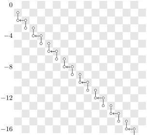
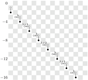
$\rho$-BSS	MASS

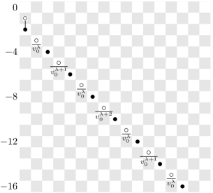
$E_{\infty}$

Figure 4. Portions of the $\rho$-BSS and MASS for $\mathsf{BP}\langle{3}\rangle_{\mathbb{Q}}$ involving $p\equiv 3\pod{4}$

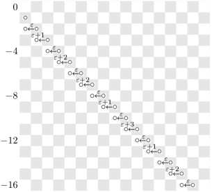
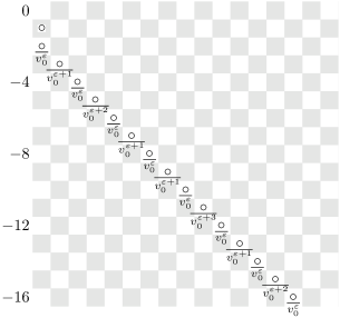
MASS	$E_{\infty}$

Figure 5. Portions of the MASS for $\mathsf{BP}\langle{3}\rangle_{\mathbb{Q}}$ involving $p\equiv 1\pod{4}$.

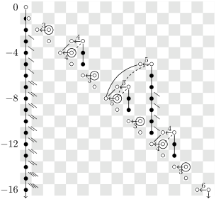
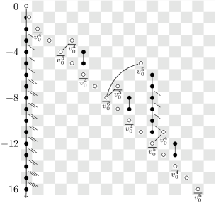
MASS	$E_{\infty}$

Figure 6. Portions of the MASS for $\mathsf{BP}\langle{3}\rangle_{\mathbb{Q}}$ involving $2$-adic and real places.

Remark 5.10.

As the reader will note, the most interesting action in the computation takes place when the real and 2-adic places intermingle. Note that a $d_{r}$ differential on a $v_{0}(j)$ class produces $v_{0}^{r+1}$-torsion in the target. This happens because $v_{0}(j)$ is in Adams filtration 1, not 0.

Consider, though, what happens to a class like $[2]\tau^{3}$ and its $v_{i}(j)$-multiples. (Note that $[2]\tau^{3}$ can be located in degree $3-4\alpha$ in the MASS portion of Figure 6.) We have a differential $d_{4}(v_{0}(2))=[2]\tau^{3}v_{0}^{5}$, making $[2]\tau^{3}$ a $v_{0}^{5}$-torsion class. We also have $d_{4}(v_{1}(1))=[2]\tau^{3}v_{0}^{4}v_{1}$, so $[2]\tau^{3}v_{1}$ is a $v_{0}^{4}$-torsion class. In this fashion, we see a $v_{1}$-multiple of a $v_{0}^{5}$-torsion class which is killed by $v_{0}^{4}$.

The above scenrio is a specific case of a general phenomenon in our computations: differentials supported by $v_{i>0}(j)$’s (those classes at the end of dashed lines in our MASS picture) will produce $v_{0}^{3+i+\nu_{2}(j)}$-torsion on $[2]\tau^{2^{i+1}j-1}v_{i}$ while $[2]\tau^{2^{i+1}j-1}$ is $v_{0}^{4+i+\nu_{2}(j)}$-torsion.

Remark 5.11.

In the dimensional range pictured, the $E_{\infty}$-pages of Figures 4, 5, and 6 almost depict $E_{\infty}$ for $\pi_{\star}\mathsf{BP}_{\mathbb{Q}}$. The only difference is that the $v_{0}^{6}$-torsion class in degree $15-16\alpha$ becomes a $v_{0}^{7}$-torsion class. This is because the class $\tau^{16}$ dies in the $\rho$-BSS for $\mathsf{BP}\langle{n}\rangle$ when $n\geq 4$ so it is $v_{0}(8)$ at height 1 that supports a $d_{6}$-differential killing $[2]\tau^{15}v_{0}^{7}$ while $[2]\tau^{15}v_{0}^{6}$ survives.

Remark 5.12.

The very careful reader will note that the target of $[p]\tau$ in the $\rho$-BSS is $(\rho^{2}+a_{p})v_{0}$ when $p\equiv 3\pod{4}$, so the $\rho$-BSS portion of Figure 4 is slightly misleading. Since $\rho v_{0}$ dies on the $E_{2}$-page, no harm is done.

Proof of Theorem 5.8.

These differentials follow from a “least energy principle” guaranteed by the Hasse principle:

For $x\in E_{2}$ of the global MASS for $\mathsf{BP}\langle{n}\rangle$ let $r$ be the smallest $r^{\prime}$ such that some $H^{\mathbb{Q}_{v}}(x)$ supports a $d_{r^{\prime}}$-differential. Then $d_{r}x=y$ for $y$ a unique lift of $d_{r}H_{\mathsf{BP}\langle{n}\rangle}(x)$.

We call this a least energy principle since the global MASS has nonzero differential on $x$ as soon as its Hasse image supports differentials, and it is a straightforward corollary of injectivity in (4).

The differentials in the Theorem follow by applying this principle to the global $E_{2}$-term determined in Theorem 5.5 and the local computations of Section 3. ∎

We now set some notation so that we can express a closed form for the additive structure of $\pi_{\star}\mathsf{BP}\langle{n}\rangle$. For $p\equiv 3\pod{4}$ let $A_{p}$ be the bigraded Abelian group with

$$(A_{p})_{-\alpha} =\mathbb{Z}_{2},$$

$$(A_{p})_{-2\alpha+2r(1-\alpha)} =\mathbb{Z}/2\text{ for }r\geq 0,$$

$$(A_{p})_{1-3\alpha+2r(1-\alpha)} =\mathbb{Z}/2^{\lambda(p)-1+\nu_{2}(2r+2)}\text{ for }r\geq 0,$$

$$(A_{p})_{k+\ell\alpha} =0\text{ otherwise}.$$

Define $A=\bigoplus_{p\equiv 3\pod{4}}A_{p}$ and let

$$A(n)=A[v_{1},\ldots,v_{n}].$$

For $p\equiv 1\pod{4}$ let $B_{p}$ be the bigraded Abelian group with

$$(B_{p})_{-\alpha} =\mathbb{Z}_{2},$$

$$(B_{p})_{-2\alpha+r(1-\alpha)} =\mathbb{Z}/2^{\varepsilon(p)+\nu_{2}(r+1)}\text{ for }r\geq 0,$$

$$(B_{p})_{k+\ell\alpha} =0\text{ otherwise}.$$

Define $B=\bigoplus_{p\equiv 1\pod{4}}B_{p}$ and let

$$B(n)=B[v_{1},\ldots,v_{n}].$$

Now define

$$C^{\prime}(n)=\mathbb{Z}_{2}[\rho,\tau^{2^{n+1}},v_{1},\ldots,v_{n},w_{i}(j)\mid 1\leq i\leq n,0\leq j]$$

subject to the relations

$$\rho v_{i} =w_{i}(0),$$

$$\rho^{2^{i+1}-1}v_{i} =0,$$

$$\rho^{2^{i+1}-2}w_{i}(j) =0,$$

$$w_{i}(j)w_{k}(\ell) =w_{i}(j+2^{k-i}\ell)w_{k}(0)\text{ if }i\leq k,$$

$$w_{i}(j) =\tau^{2^{n+1}}w_{i}(j-2^{n-i})\text{ if }j\geq 2^{n-1}.$$

(Note that the class $w_{i}(j)$ is represented by $\rho\tau^{2^{i+1}j}v_{i}$ in the MASS for $\mathsf{BP}\langle{n}\rangle$.) Also define $C^{\prime\prime}(n)$ to be the bigraded Abelian group with

$$C^{\prime\prime}(n)_{-\alpha+2r(1-\alpha)} =\mathbb{Z}_{2},$$

$$C^{\prime\prime}(n)_{1-2\alpha+2r(1-\alpha)} =\mathbb{Z}/2^{3+\nu_{2}(2r+2)}\text{ for }r\geq 0\text{ and }2^{n+1}\nmid 2r+2,$$

$$C^{\prime\prime}(n)_{1-2\alpha+2r(1-\alpha)} =\mathbb{Z}/2^{2+\nu_{2}(2r+2)}\text{ for }r\geq 0\text{ and }2^{n+1}\mid 2r+2.$$

Let $t_{j}$ denote the generator of $C^{\prime\prime}(n)$ in degree $-\alpha+j(1-\alpha)$ and define

$$C^{\prime\prime\prime}(n)=C^{\prime\prime}(n)[v_{1},\ldots,v_{n}]/(2^{2+\nu_{2}(j+1)}t_{j}v_{i}\mid j\equiv 3\pod{4},1\leq i\leq\nu_{2}(j+1)-1).$$

We define

$$C(n)=C^{\prime}(n)\oplus C^{\prime\prime\prime}(n).$$

Note that $A(n)$, $B(n)$, and $C(n)$ capture precisely the information on the $E_{\infty}$ pages presented in Figures 4, 5, and 6, respectively, once $v_{0}=2$ is taken into account. The following result is now a direct consequence of Theorem 5.8.

Theorem 5.13.

The coefficients of $\mathsf{BP}\langle{n}\rangle$ over $\mathbb{Q}$ take the form

$$\pi_{\star}\mathsf{BP}\langle{n}\rangle=A(n)\oplus B(n)\oplus C(n)$$

additively.

Remark 5.14.

By Lemma 2.9 in the $n=1$ case we can recover the Rognes-Weibel [23] computation of the 2-complete algebraic $K$-theory of $\mathbb{Q}$ by inverting $v_{1}$ and looking at the weight $0$ piece of the coefficients.

Remark 5.15.

Recall Quillen’s localization fiber sequence for 2-complete algebraic $K$-theory spectra

$$\bigvee_{p}K\mathbb{F}_{p}\to K\mathbb{Z}\to K\mathbb{Q}.$$

The associated long exact sequence on homotopy groups splits into isomorphisms $K_{2i}\mathbb{Z}\cong K_{2i}\mathbb{Q}$ and split short exact sequences

$$0\to K_{2i+1}\mathbb{Z}\to K_{2i+1}\mathbb{Q}\to\bigoplus_{p}K_{2i}\mathbb{F}_{p}\to 0$$

for $i\geq 1$. In the $n=1$ case, after inverting $v_{1}$ we see that the decomposition in Theorem 5.13 respects the localization decomposition of $K_{*}\mathbb{Q}$ in the following sense:

$$v_{1}^{-1}A(1)_{m}\oplus v_{1}^{-1}B(1)_{m} \cong\bigoplus_{p}K_{m-1}\mathbb{F}_{p},$$

$$v_{1}^{-1}C(1)_{m} \cong K_{m}\mathbb{Z}$$

abstractly for $m\geq 2$.

Let $\mathsf{E}(n)=v_{n}^{-1}\mathsf{BP}\langle{n}\rangle$ denote the motivic Johnson-Wilson spectrum. (Note that $\mathsf{E}(1)=\mathsf{KGL}$ in the 2-complete category.) We can ask then whether there are integral models of the rational and $\mathbb{F}_{p}$ truncated Brown-Peterson and Johnson-Wilson spectra so that there are localization fiber sequences

$$\bigvee_{p}\mathsf{BP}\langle{n}\rangle_{\mathbb{F}_{p}}^{\mathbb{Z}}\to\mathsf{BP}\langle{n}\rangle_{\mathbb{Z}}\to\mathsf{BP}\langle{n}\rangle_{\mathbb{Q}}^{\mathbb{Z}},$$

$$\bigvee_{p}\mathsf{E}(n)_{\mathbb{F}_{p}}^{\mathbb{Z}}\to\mathsf{E}(n)_{\mathbb{Z}}\to\mathsf{E}(n)_{\mathbb{Q}}^{\mathbb{Z}}$$

in the category of motivic spectra over $\operatorname{Spec}\mathbb{Z}$. Joseph Ayoub has informed us that these sorts of localization sequences should be related to Quillen purity theorems for $\mathsf{BP}\langle{n}\rangle$ and $\mathsf{E}(n)$. Such results should follow from purity for algebraic $K$-theory in the $n=1$ case but $n>1$ is terra incognita.

On the basis of our MASS computations over $\mathbb{Q}$, we might wildly speculate that the MASS for $\mathsf{BP}\langle{n}\rangle_{\mathbb{Z}}$ would match portion of the MASS for $\mathsf{BP}\langle{n}\rangle_{\mathbb{Q}}$ presented in Figure 6 and the MASS for $\mathsf{BP}\langle{n}\rangle_{\mathbb{F}_{p}}$ would match the portion of the MASS for $\mathsf{BP}\langle{n}\rangle_{\mathbb{Q}}$ presented in Figure 4 or 5 (depending on whether $p\equiv 3$ or $1\pod{4}$, respectively). That said, essentially nothing is known about the structure of $\mathcal{A}_{\star}$ or convergence of the MASS over $\mathbb{Z}$.

By working in the stable motivic homotopy category over $\mathbb{F}_{p}$, the authors have currently verified that the MASS for $\mathsf{BP}\langle{n}\rangle_{\mathbb{F}_{p}}$, $p>2$, does indeed behave this way [20]. (Work of Mark Hoyois, Sean Kelly, and the second author [5] identifies the dual motivic Steenrod algebra at 2 over $\mathbb{F}_{p}$ for $p>2$, which then permits methods similar to those in Section 3 of this paper to be applied.) The MASS for $\mathsf{BP}\langle{n}\rangle_{\mathbb{F}_{2}}$ remains mysterious.

References

- [1] S. Borghesi. Algebraic Morava -theories. Invent. Math., 151(2):381–413, 2003.
- [2] D. Dugger and D. C. Isaksen. The motivic Adams spectral sequence. Geom. Topol., 14(2):967–1014, 2010.
- [3] M. A. Hill. Ext and the motivic Steenrod algebra over . J. Pure Appl. Algebra, 215(5):715–727, 2011.
- [4] M. Hoyois. From algebraic cobordism to motivic cohomology. arXiv:1210.7182.
- [5] M. Hoyois, S. Kelly, and P. A. Østvær. The motivic Steenrod algebra over perfect fields. Preprint, 2012.
- [6] P. Hu. On Real-oriented Johnson-Wilson cohomology. Algebr. Geom. Topol., 2:937–947, 2002.
- [7] P. Hu and I. Kriz. Some remarks on Real and algebraic cobordism. -Theory, 22(4):335–366, 2001.
- [8] P. Hu, I. Kriz, and K. Ormsby. Convergence of the motivic Adams spectral sequence. J. K-Theory, 7(3):573–596, 2011.
- [9] P. Hu, I. Kriz, and K. Ormsby. Remarks on motivic homotopy theory over algebraically closed fields. J. K-Theory, 7(1):55–89, 2011.
- [10] J. Milnor. The Steenrod algebra and its dual. Ann. of Math. (2), 67:150–171, 1958.
- [11] J. Milnor. Algebraic -theory and quadratic forms. Invent. Math., 9:318–344, 1969/1970.
- [12] F. Morel. An introduction to -homotopy theory. In Contemporary developments in algebraic -theory, ICTP Lect. Notes, XV, pages 357–441 (electronic). Abdus Salam Int. Cent. Theoret. Phys., Trieste, 2004.
- [13] F. Morel. The stable -connectivity theorems. -Theory, 35(1-2):1–68, 2005.
- [14] F. Morel and V. Voevodsky. -homotopy theory of schemes. Inst. Hautes Études Sci. Publ. Math., (90):45–143 (2001), 1999.
- [15] N. Naumann, M. Spitzweck, and P. A. Østvær. Existence and uniqueness of -structures on motivic K-theory spectra. arXiv:1010.3944.
- [16] N. Naumann, M. Spitzweck, and P. A. Østvær. Chern classes, -theory and landweber exactness over nonregular base schemes. In Motives and Algebraic Cycles: A celebration in Honour of Spencer J. Bloch, Fields Institute Communications, Vol. 56, pages 307–317. AMS, Providence, RI, 2009.
- [17] N. Naumann, M. Spitzweck, and P. A. Østvær. Motivic Landweber exactness. Doc. Math., 14:551–593 (electronic), 2009.
- [18] J. Neukirch, A. Schmidt, and K. Wingberg. Cohomology of number fields, volume 323 of Grundlehren der Mathematischen Wissenschaften [Fundamental Principles of Mathematical Sciences]. Springer-Verlag, Berlin, second edition, 2008.
- [19] K. Ormsby. Motivic invariants of -adic fields. J. K-Theory, 7(3):597–618, 2011.
- [20] K. Ormsby and P. A. Østvær. Motivic invariants of low-dimensional fields. In preparation.
- [21] D. Quillen. On the formal group laws of unoriented and complex cobordism theory. Bull. Amer. Math. Soc., 75:1293–1298, 1969.
- [22] D. C. Ravenel. Complex cobordism and stable homotopy groups of spheres, volume 121 of Pure and Applied Mathematics. Academic Press Inc., Orlando, FL, 1986.
- [23] J. Rognes and C. Weibel. Two-primary algebraic -theory of rings of integers in number fields. J. Amer. Math. Soc., 13(1):1–54, 2000. Appendix A by Manfred Kolster.
- [24] O. Röndigs and P. A. Østvær. Motives and modules over motivic cohomology. C. R. Math. Acad. Sci. Paris, 342(10):751–754, 2006.
- [25] O. Röndigs and P. A. Østvær. Modules over motivic cohomology. Adv. Math., 219(2):689–727, 2008.
- [26] M. Spitzweck. Relations between slices and quotients of the algebraic cobordism spectrum. Homology, Homotopy Appl., 12(2):335–351, 2010.
- [27] A. A. Suslin. On the -theory of local fields. In Proceedings of the Luminy conference on algebraic -theory (Luminy, 1983), volume 34, pages 301–318, 1984.
- [28] G. Vezzosi. Brown-Peterson spectra in stable -homotopy theory. Rend. Sem. Mat. Univ. Padova, 106:47–64, 2001.
- [29] V. Voevodsky. -homotopy theory. In Proceedings of the International Congress of Mathematicians, Vol. I (Berlin, 1998), number Extra Vol. I, pages 579–604 (electronic), 1998.
- [30] V. Voevodsky. Motivic cohomology with -coefficients. Publ. Math. Inst. Hautes Études Sci., (98):59–104, 2003.
- [31] V. Voevodsky. Reduced power operations in motivic cohomology. Publ. Math. Inst. Hautes Études Sci., (98):1–57, 2003.
- [32] V. Voevodsky. Motivic Eilenberg-Maclane spaces. Publ. Math. Inst. Hautes Études Sci., (112):1–99, 2010.
- [33] N. Yagita. Applications of Atiyah-Hirzebruch spectral sequences for motivic cobordism. Proc. London Math. Soc. (3), 90(3):783–816, 2005.