Mixedness and entanglement for two-mode Gaussian states

Resumo

We analytically exploit the two-mode Gaussian states nonunitary dynamics. We show that in the zero temperature limit, entanglement sudden death (ESD) will always occur for symmetric states (where initial single mode compression is $z_{0}$) provided the two mode squeezing $r_{0}$ satisfies $0<r_{0}<\frac{1}{2}\log(\cosh(2z_{0})).$ We also give the analytical expressions for the time of ESD. Finally, we show the relation between the single modes initial impurities and the initial entanglement, where we exhibit that the later is suppressed by the former.

I Introduction

The concept of entanglement, a typically quantum mechanical property, is a natural consequence of the superposition principle for composite systems. It was discussed by Schrödinger who immediately realized its (at the time) seemingly “unphysical” consequences schrodinger . Nowadays the growing interest in the subject is related to quantum information theory and potential technological applications esd ; Bacon-Phys . Thus a lot of effort has been put both in the quantification of entanglement and in studying the consequences of deleterious environmental effects on this property decoherence . It is well known today, both theoretically and experimentally, that in general such effects tend to destroy quantum properties; in the case of systems with one degree of freedom this happens only asymptotically leocarol1 ; leocarol2 ; adesso1 . The studies concerning the degradation of quantum effects are vast in the literature, specially those related to continuous variables systems subjected to noisy channels, see cite1 ; cite2 . Some recent works devote their attention to the robustness of Gaussian and non-Gaussian states under dissipative channels cite3 .

It was recently realized that in bipartite systems that entanglement may disappear suddenly, phenomenon called therefore “entanglement sudden death” (ESD) or finite-time disentanglement esdcv ; PR . The phenomenon is strongly related to geometrical properties of the set of mixed quantum states GeoSudDeath , but from a physical point of view, the issue is still far from being closed.

In the present work we study more specifically the entanglement properties of two mode Gaussian states under a nonunitary evolution. In ref. leocarol1 ; leocarol2 ; adesso1 the entropy growth of single-mode Gaussian and non-Gaussian states coupled to a reservoir has been presented in analytical form. We show that in the two-mode case, single-mode squeezing plays an important role in entanglement dynamics, even for fully symmetric channels (phenomenon that appears also in the case of qu-bits marcelin ). For the specific case of a zero temperature reservoir and symmetric states (where initial single mode squeezing of both modes is $z_{0}$) we are able wo show that ESD will always occur if $0<r_{0}<\frac{1}{2}\log(\cosh(2z_{0}))$, where $r_{0}$ is the two mode squeezing. We also show that there exists an upper limit for the degree of mixedness of a state so that it can exhibit entanglement. This result may turn out useful for experimental realizations of two-mode entangled Gaussian states. Finally, for symmetric and pure states evolving in a reservoir at zero temperature, we analytically present the time of ESD.

The paper is organized as follows: in section II we present some well known properties concerning Gaussian States; in the next section we briefly review the analytical dynamics of two-mode Gaussian states; in section IV we present our results. Finally, some conclusions are drawn.

II General properties of two-mode Gaussian states

A two-mode Gaussian state with vanishing averages $\langle{a}_{i}\rangle=\operatorname{tr}(a_{i}\rho)=0$, $i=1,2$, can always be written as

$$\rho_{G}=S_{1}(z_{1},z_{2})S_{2}(r)\mathbf{\sigma}(\nu_{1},\nu_{2})S_{2}^{\dagger}(r)S_{1}^{\dagger}(z_{1},z_{2}),$$ (1)

where $S_{1}(z_{1},z_{2})$ is the single mode squeezing operator, $S_{2}(r)$ is the two-mode squeezing operator and $\mathbf{\sigma}(\nu_{1},\nu_{2})$ is the two-mode thermal state. More explicitly we have:

$$S_{1}(z_{1},z_{2}) = \exp\left[\frac{z_{1}}{2}(a_{1}^{\dagger 2}-a_{1}^{2})\right]\exp\left[\frac{z_{2}}{2}(a_{2}^{\dagger 2}-a_{2}^{2})\right],$$ (2)

$$S_{2}(r) = \exp\left[r(a_{1}^{\dagger}a_{2}^{\dagger}-a_{1}a_{2})\right],$$ (3)

$$\mathbf{\sigma}(\nu_{1},\nu_{2}) = \frac{1}{\nu_{1}+1}\frac{1}{\nu_{2}+1}\sum_{n}\sum_{m}\left(\frac{\nu_{1}}{\nu_{1}+1}\right)^{n}\left(\frac{\nu_{2}}{\nu_{2}+1}\right)^{m}\left|n\right\rangle\left\langle n\right|\otimes\left|m\right\rangle\left\langle m\right|,$$

where $z_{i}$ is the single-mode squeezing parameter of the mode $i$, $a_{i}^{(\dagger)}$ is the annihilation (creation) operator of the $i-$th mode, $r$ is the two-mode squeezing and $\nu_{i}$ is the “mixedness” of the $i-$th mode (by “mixedness” we mean the initial number of thermal photons of the state), related of the thermal two-mode state $\mathbf{\sigma}$. We assume $\langle a_{i}\rangle=0$ in this work, since the entanglement properties are independent of them, and in our equations of motion the second momenta evolution decouple form the first momenta. We also choose, without loss of generality in this case, the squeezing parameters $z_{i}$ and $r$ to be real.

This state is entirely described by the parameters given above. However, in order to handle entanglement properties, it is most convenient to write these parameters in terms of the corresponding covariance matrix (CM):

$$V_{{\rho}}=\left(\begin{array}[]{cccc}n_{1}+\frac{1}{2}&m_{1}&m_{s}&m_{c}\\ m_{1}^{*}&n_{1}+\frac{1}{2}&m_{c}^{*}&m_{s}^{*}\\ m_{s}^{*}&m_{c}&n_{2}+\frac{1}{2}&m_{2}\\ m_{c}^{*}&m_{s}&m_{2}^{*}&n_{2}+\frac{1}{2}\end{array}\right),$$ (8)

where $n_{i}=\langle{a}^{\dagger}_{i}{a}_{i}\rangle$, $m_{i}=-\langle{a}_{i}^{2}\rangle$, $m_{s}=-\langle{a}_{1}{a}_{2}^{\dagger}\rangle$, $m_{c}=\langle{a}_{1}{a}_{2}\rangle$, and $\langle{\xi}\rangle$ denotes the quantum expectation value $\operatorname{tr}({\xi}{\rho})$ of an observable ${\xi}$. The CM can also be written as

$$V_{{\rho}}=\left(\begin{array}[]{cc}V_{1}&C\\ C^{\dagger}&V_{2}\end{array}\right),$$ (11)

where $V_{i}$ is a $2\times 2$ matrix related to the mode $i$, and $C$ is a $2\times 2$ matrix that gives the correlations (both quantum and classical) between the modes. For later use, we define some invariants of the covariance matrix as adesso1 ; haruna :

$$I_{V} = \det V_{\rho},$$

$$I_{1,2} = \det V_{1,2},$$

$$I_{3} = \det C,$$

$$I_{4} = \operatorname{tr}\left[V_{1}ZCZV_{2}ZC^{\dagger}Z\right].$$ (12)

These quantities are invariants under local unitary operations and $Z=\text{diag}\{1,-1\}$. Next we give the explicit connection between the parameters of the Gaussian state and the matrix elements of the covariance matrix:

$$z_{i} = \frac{1}{2}\mathrm{arctanh}\left[\frac{m_{i}}{n_{i}+\frac{1}{2}}\right]$$ (13)

$$\nu_{1} = \frac{1}{2}\left(\det V_{1}-\det V_{2}\right)+$$ (14)

$$+\frac{1}{2}\sqrt{1-x^{2}}\left(\det V_{1}+\det V_{2}\right)-\frac{1}{2},$$

$$\nu_{2} = \frac{1}{2}\left(\det V_{2}-\det V_{1}\right)+$$ (15)

$$+\frac{1}{2}\sqrt{1-x^{2}}\left(\det V_{1}+\det V_{2}\right)-\frac{1}{2},$$

$$r = \frac{1}{2}\mathrm{arctanh}\left[x\right],$$ (16)

where we have defined

$$x=\frac{2m_{s}}{(\sqrt{\det V_{1}}+\sqrt{\det V_{2}})\sinh(z_{1}+z_{2})}.$$ (17)

Once the evolution of the covariance matrix is obtained, the evolution of the parameters of the state can be inferred.

Since we are working with Gaussian states, there are necessary and sufficient criterion to determine if the state is entangled simon ; DGCZ ; serafini1 . Simon simon has shown that for any two-mode Gaussian state, if the following inequality is observed

$$S\left(V_{\hat{\rho}}\right)=I_{1}I_{2}+(1/4-|I_{3}|)^{2}-I_{4}-1/4(I_{1}+I_{2})\geq 0,$$ (18)

the state is separable. For the purposes of this work, Simon’s criterion is enough to study the entanglement dynamics.

III Nonunitary dynamics and its analytical solution

The degradation of the quantum information content of Gaussian states is a subject of interest, both for the technological and/or experimental applications as well as for fundamental quantum mechanics in what concerns the classical limit.

The usual approach to non-unitary dynamics is by means of master equations, which has found several successful applications in other areas of physics. Our master equation reads

$$\dot{\rho}=\mathcal{L}\rho,$$ (19)

where $\mathcal{L}$ is a superoperator given by:

$$\mathcal{L} = \sum_{i=1,2}\left(\gamma_{i}(n_{i}^{B}+1)(2a_{i}\bullet a_{i}^{\dagger}-a_{i}^{\dagger}a_{i}\bullet-\bullet a_{i}^{\dagger}a_{i})+\gamma_{i}\leavevmode\nobreak\ n_{i}^{B}(2a_{i}^{\dagger}\bullet a_{i}-a_{i}a_{i}^{\dagger}\bullet-\bullet a_{i}a_{i}^{\dagger})\right).$$ (20)

In the equation above, $\gamma_{i}$ is the dissipation constant of the reservoir related to the mode $i$, $\bar{n}_{i}^{B}$ is related to the temperature of the thermal bath of the mode $i$, and $a_{i}^{\dagger}(a_{i})$ is the creation (annihilation) operator of the respective mode.

The equation (20) models a linear coupling between the state (the two-mode Gaussian state in our case) with a thermal bath of quantum harmonic oscillators. The evolution of each term of the covariance matrix, evolving under the dynamics described above, is given by:

$$n_{i} = \mathrm{e}^{-2t\gamma_{i}}\left(\left(-1+e^{2t\gamma_{i}}\right)n_{i}^{B}+\cosh(2z_{i}^{0})\left(\nu_{i}^{0}\cosh^{2}r_{0}+(1+\nu_{k}^{0})\sinh^{2}r_{0}\right)+\sinh^{2}z_{i}^{0}\right);$$ (21)

$$m_{i} = -\mathrm{e}^{-2t\gamma_{i}}(\nu_{i}^{0}-\nu_{k}^{0}+(1+\nu_{i}^{0}+\nu_{k}^{0})\cosh(2r_{0}))\cosh z_{i}^{0}\sinh z_{i}^{0};$$ (22)

$$m_{c} = \frac{1}{2}\mathrm{e}^{-t(\gamma_{1}+\gamma_{2})}(1+\nu_{1}^{0}+\nu_{2}^{0})\cosh(z_{1}^{0}+z_{2}^{0})\sinh(2r_{0});$$ (23)

$$m_{s} = -\frac{1}{2}\mathrm{e}^{-t(\gamma_{1}+\gamma_{2})}(1+\nu_{1}^{0}+\nu_{2}^{0})\sinh(2r_{0})\sinh(z_{1}^{0}+z_{2}^{0}).$$ (24)

In the equations above, $i=1$ or $2$ (mode 1 or mode 2) and $k\neq i$. The parameters are such that $z_{i}^{0}$ is the initial single mode squeezing, $\gamma_{i}$ is the dissipation constant, $\nu_{i}^{0}$ is related to the initial mixedness and $n_{i}^{B}$ is the reservoir temperature, where all the quantities refer to the $i-$th mode, as denoted by the suscript $i$. Also, we have that $r_{0}$ is the initial two-mode squeezing.

IV Results

IV.1 Entanglement dynamics and single mode squeezing

In order to get a clear picture and to gain physical insight into the rich and multifaceted aspects of the non-unitary dynamics of general two-mode Gaussian states, we consider firstly the simplest case, i.e. the two-mode squeezed vacuum in dissipative channel.

Let us consider the case of a two-mode vacuum state without single-mode squeezing (i.e. $z_{1}=z_{2}=0$). As shown in Figure 1, for symmetric and asymmetric channels, with temperatures $n_{1}^{B}$ and $n_{2}^{B}$ different from zero, there will always be a finite time when entanglement vanishes. This can be understood using a geometrical picture of entanglement decay GeoSudDeath . In fact, in this case, the long-time state is a separable mixed state, well within the set of separable states. Thus, if an initial state is entangled, it necessarily crosses the border of separable states in finite time. For zero-temperature baths, i.e. if $n_{1}^{B}=n_{2}^{B}=0$, even if one uses different dissipation constants $\gamma_{1}$ and $\gamma_{2}$, the entanglement only disappears asymptotically.

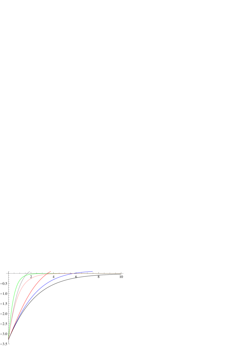
Figura 1: Simon criterion for several cases of initial parameters. The common parameters are: $z_{1}^{0}=z_{2}^{0}=\nu_{1}^{0}=\nu_{2}^{0}=0,r_{0}=1$. In each curve: gray: $\gamma_{1}=0.1,\gamma_{2}=0.5,n_{1}=0.2,n_{2}=0.2$; blue: $\gamma_{1}=0.1,\gamma_{2}=0.1,n_{1}=0.2,n_{2}=0.2$; green: $\gamma_{1}=0.5,\gamma_{2}=0.5,n_{1}=0.0,n_{2}=0.0$; red: $\gamma_{1}=0.1,\gamma_{2}=0.1,n_{1}=1.0,n_{2}=0.0$; black: $\gamma_{1}=0.1,\gamma_{2}=0.1,n_{1}=0.0,n_{2}=0.0$; pink: $\gamma_{1}=0.1,\gamma_{2}=0.5,n_{1}=0.0,n_{2}=0.0$.

Next we introduce single mode squeezing, i.e. $z_{1}^{0}\neq 0$ and/or $z_{2}^{0}\neq 0$. We note in Figure 2 that, even for the zero temperature case, one observes entanglement sudden death (ESD). We note that there is a dynamical entropy increase of the squeezed mode, caused by the reservoir, which acts in such a way that, for a relatively short time interval, this mode’s entropy grows and then decays to the vacuum. We have observed that this dynamical entropy growth leocarol1 ; leocarol2 causes the entanglement disappearance in finite time.

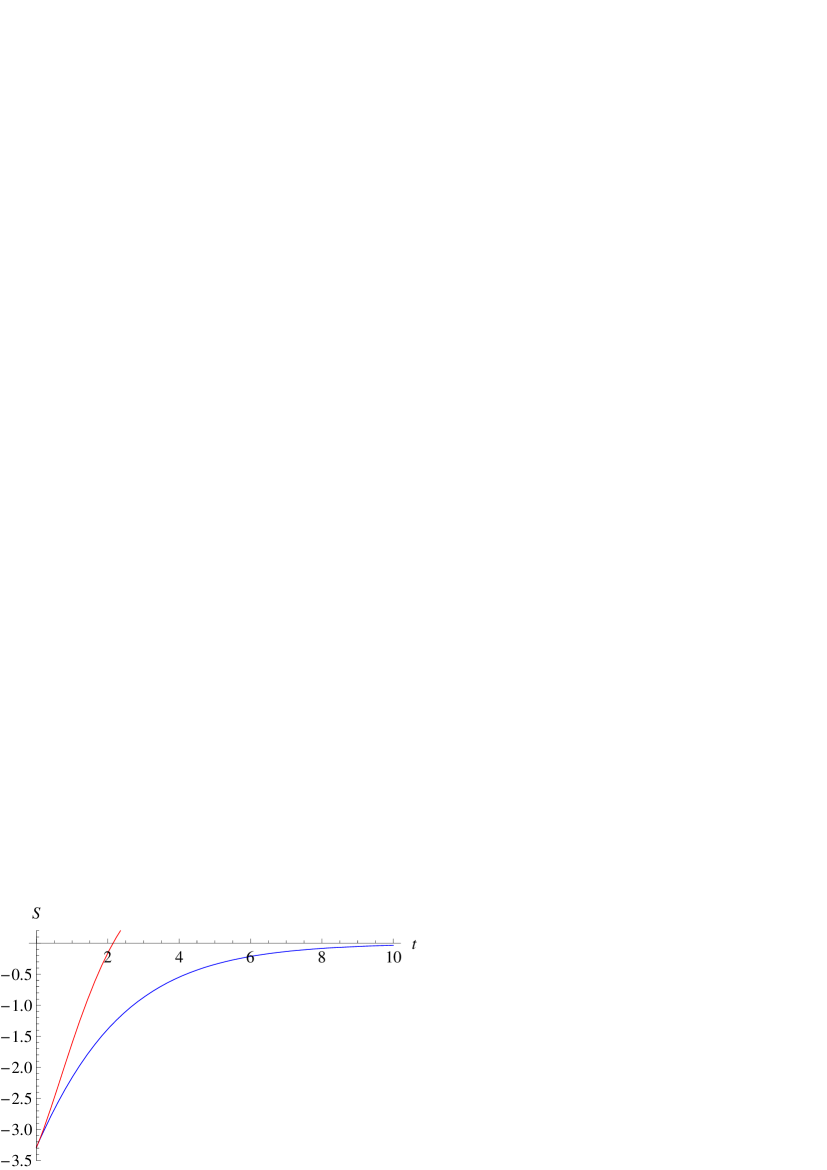
Figura 2: Simon criterion for two set of initial parameters, say: $\nu_{1}^{0}=\nu_{2}^{0}=0,r_{0}=1$. Blue: $\gamma_{1}=\gamma_{2}=0.1,n_{1}^{B}=n_{2}^{B}=0,z_{1}^{0}=z_{2}^{0}=0$; Red: $\gamma_{1}=\gamma_{2}=0.1,n_{1}^{B}=n_{2}^{B}=0,z_{1}^{0}=2,z_{2}^{0}=0.$

Since single-mode squeezing turns out to play a significant role on ESD. In Figure 3 we show Simon’s criterion evolution for states with compression in only one of the modes, for reservoirs at null temperature. The vertical axis corresponds to the initial parameter $z_{1}^{0}$ and the plot shows, for each instant of time, whether the evolved state is entangled (shaded area) or not (blank area). For instance, if the initial state has $z_{1}^{0}=2$, Simon’s criterion will change from negative to positive in finite time; if one have $z_{1}^{0}=1.0$, the entanglement will vanish asymptotically. We will show an analytical relation between single-mode squeezing and ESD hereafter.

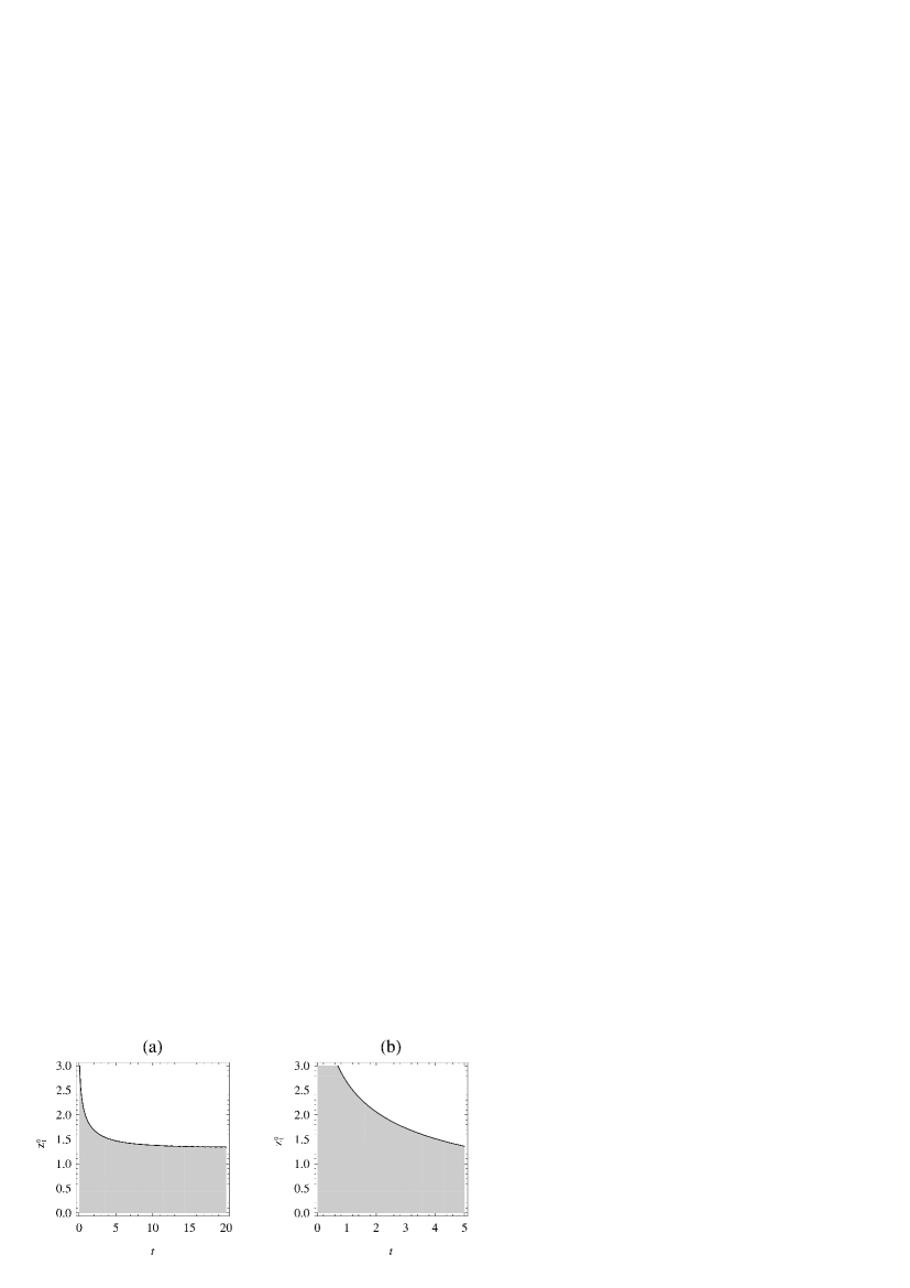
Figura 3: Simon criterion for values of the initial parameter $z_{1}^{0}$ and time $t$, where we have used $z_{1}^{0}=z_{2}^{0}$. For the shaded area the Simon criterion $S$ is negative (entangled state), in the white area $S$ is positive. Note that there is a limit for $z_{1}$ in which the state will have ESD. In this case: $z_{1}\simeq 1.4$. Parameters: $r_{0}=1,\nu_{1}^{0}=\nu_{2}^{0}=0,n_{1}^{B}=n_{2}^{B}=0,\gamma_{1}=\gamma_{2}=0.1.$ Graphs (a) and (b) are the same function, in a different time scale.

In the following we want to discuss the instant of time in which the state becomes separable, or when occurs ESD, in the case of zero temperature and symmetrical states ($z_{i}^{0}=0$, $r_{0}>0$, $\nu_{i}^{0}$=$\nu_{0}$ and $\gamma_{i}=\gamma$, $n_{i}^{B}=0$, for $i=1,2$). In this case the elements of the covariance matrix, which do not vanish, depend on

$$n =n(t)=\frac{1}{2}e^{-2\gamma t}((2\nu_{0}+1)\cosh(2r_{0})-1)=n_{0}e^{-2\gamma t},$$ (25)

$$m =m(t)=\frac{1}{2}e^{-2\gamma t}(2\nu_{0}+1)\sinh(2r_{0})=m_{0}e^{-2\gamma t}.$$ (26)

In this case Simon $S$ can be factorized as $S=(m+n)(m+n+1)(m-n)(m-n-1)$. Since the first two factors are clearly positive, we can see that $S$ is negative if $n<m<n+1$. If this inequality is satisfied at the initial time, $n_{0}<m_{0}<n_{0}+1$. Now, multiplying by $e^{-2\gamma t}$ we get $n<m<n+e^{-2\gamma t}<n+1$. Thus, if the state is initially entangled, the evolved state is also entangled for any finite time. Since Simon $S$ vanishes asymptotically $\lim_{t\rightarrow\infty}S(t)=0$, we see that either the entanglement decay is asymptotic, or the initial state is already separable. A two-mode squeezed vacuum, $\nu_{0}=0$, is always entangled; hence, it separates asymptotically.

Now we study $t_{ESD}$ for states containing single-mode squeezing, i.e. $z_{1}=z_{2}$. Here one can find for $t_{ESD}$:

$$\mathrm{e}^{-2\gamma t_{ESD}}=\frac{2\exp(r_{0})\cosh 2z_{0}\sinh r_{0}-2\sinh^{2}z_{0}}{\exp(2r_{0})(\cosh 2r_{0}-\sinh 2z_{0})},$$ (27)

where we consider $r_{0}>0$, and $z_{1}^{0}=z_{2}^{0}=z_{0}$. In terms of the new variables $\eta=\exp(2r_{0})$ and $\zeta=\exp(2z_{0})$, the disentanglement time

$$\mathrm{e}^{-2\gamma t_{ESD}}=\frac{\eta(1+\zeta^{2}-2\eta\zeta)}{\eta-\zeta-\eta^{2}\zeta+\zeta^{2}\eta},$$

is much easier to analyze. This equation has a valid solution when the right-hand side varies between 0 and 1, that is, when $\eta$ satisfies the inequality $1\leq\eta\leq\frac{1}{2}\left(\zeta+\frac{1}{\zeta}\right)$. Going back to the original variables we conclude that the initial state separates at a finite time if $0<r_{0}<\frac{1}{2}\log\left(\cosh(2z_{0})\right)$. In this case, one can see clearly that the effect of single-mode squeezing is crucial to determine when the entangle will vanish.

IV.2 Effects of the mixedness in the initial state

Recently leocarol1 ; leocarol2 it has been shown that in the case of single mode Gaussian states, there is an upper limit for the degree of global purity (represented by $\nu_{i}^{0}$) of the state above which no quantum properties are visible. We now show that an analogous result holds for two mode Gaussian systems also. Following the steps in ref. leocarol1 ; leocarol2 we can show that the initial state is entangled if the following inequality is satisfied:

$$r_{0}>\frac{1}{4}\cosh^{-1}\left(\frac{(1+\nu_{2}^{0})^{2}+2\nu_{1}^{0}(1+\nu_{2}^{0})(1+4\nu_{2}^{0})+(\nu_{1}^{0})^{2}(1+8\nu_{2}^{0}(1+\nu_{2}^{0}))}{(1+\nu_{1}^{0}+\nu_{2}^{0})^{2}}\right).$$ (28)

In Figure 4 we show the entanglement in the initial state as measured by $S$, with $r_{0}=1$. Notice that there is an upper limit on the initial state impurity above which the state becomes separable.

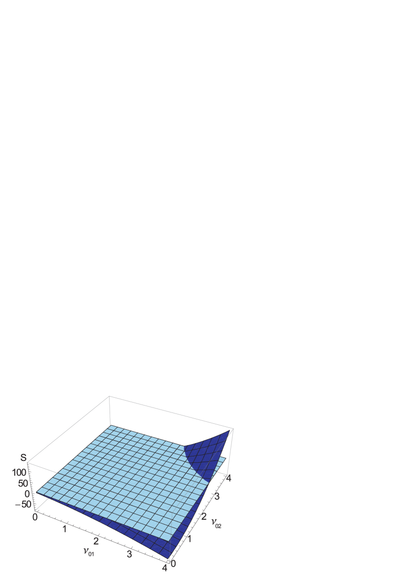
Figura 4: Simon criterion for the two-mode Gaussian state, equation (1). Note that impurities values sufficiently high can suppress the effect of entanglement given by the two-mode squeezing parameter $r$. Parameter: $r_{0}=1$.

V Conclusion

In this paper we review some aspects of two-mode Gaussian states, showing both the evolution of the state parameters (that entirely characterize the state) under nonunitary evolution and how entanglement of the state, characterized by the Simon criterion (18), depends on the initial state parameters. We show that, even in completely symmetrical reservoirs and zero temperature, the entanglement can vanish in finite time, depending on the single-mode squeezing of the state. We give a condition for ESD relating single mode squeezing and two mode squeezing, that is $0<r_{0}<\frac{1}{2}\log(\cosh(2z_{0}))$. We analytically present the time when occurs ESD for symmetrical states, evolving in a reservoir with zero temperature. We also show that entanglement can be “suppressed” by the initial mixedness of the modes, $\nu_{i}^{0}$: the initial two mode squeezing has an upper limit as a function $\nu_{i}^{0}$, and for values above this limit the state is separable. This can be helpful for experimental procedures, since any state will have some minimal impurity.

Acknowledgements - L.A.M. Souza thanks FAPEMIG for financial support. L.A.M. Souza also thanks F. Toscano and F. Nicácio for fruitful discussions and suggestion that they have made in the III Workshop of Quantum Information (Paraty - $2011$).

- (1) E. Schrödinger, Proc. of the Camb. Phil. Soc., 31 555 (1935); E. Schrödinger, Proc. of the Camb. Phil. Soc., 32 446 (1936)
- (2) K. Życzkowski, P. Horodecki, M. Horodecki, and R. Horodecki, Phys. Rev. A65, 012101 (2001); T. Yu and J. H. Eberly, Phys. Rev. B66, 193306 (2002); L. Diósi, Lect. Notes Phys. 622, 157 (2003); P. J. Dodd and J. J. Halliwell, Phys. Rev. A69, 052105 (2004); T. Yu and J. H. Eberly, Opt. Commun. 264, 393 (2006); A. Salles, F. Melo, M. P. Almeida, M. Hor-Meyll, S. P. Walborn, P. H. Souto Ribeiro, L. Davidovich, Phys. Rev. A 78, 022322 (2008); M. P. Almeida, F. de Melo, M. Hor-Meyll, A. Salles, S. P. Walborn, P. H. S. Ribeiro, and L. Davidovich, Science 316, 579 (2007).
- (3) D. Gross, S. T. Flammia, and J. Eisert, Phys. Rev. Lett. 102, 190501 (2009); M. J. Bremmer, C. Mora, and A. Winter, Phys. Rev. Lett. 102, 190502 (2009); D. Bacon, Physics 2, 38 (2009).
- (4) W. H. Zurek, Decoherence, einselection, and the quantum origins of the classical, Rev. of Mod. Phys., 75, 715, (2003); E. Joos, H. Zeh, C. Kiefer, D. Giulini, J. Kupsch, and I.-O. Stamatescu, Decoherence and the Appearance of a Classical World in Quantum Theory (Springer, 2003).
- (5) L. A. Mendes de Souza, M. C. Nemes, Physics Letters A. , 372, 3616, (2008).
- (6) L. A. Mendes de Souza, M. C. Nemes, M. França Santos, J. G. Peixoto de Faria, Optics Communications , 281, 4696, (2008).
- (7) G. Adesso, A. Serafini and F. Illuminati, Phys. Rev. A70 022318 (2004); Phys. Rev. Lett. 93 220504 (2004); G. Adesso, PhD. Thesis, Universitá di Salerno (2006), arXiv:quant-ph/0702069.
- (8) J. Laurat et al, Jour. of Opt. B 7 S577 (2005); R. C. Drumond; L. A. M. Souza;M. Terra Cunha, Phys. Rev. A82 042302 (2010); M. G. A. Paris, F. Illuminati, A. Serafini and S. De Siena, Phys. Rev. A68 012314 (2003); A. Serafini, G. Adesso, and F. Illuminati, Phys. Rev. A71 032349 (2004); G. Adesso, A. Serafini, and F. Illuminati, Open Sys. Inf. Dyn. 12 189 (2005); G. Adesso, F. Illuminati, J. Phys. A 40, 7821 (2007); A. Monras, F. Illuminati, http://arxiv.org/abs/1010.0442v1.
- (9) P. Marian and T. A. Marian, Phys. Rev. Lett. 101 220403 (2008); A. S. M. de Castro and V. V. Dodonov, Phys. Rev. A73 065801 (2006); A. Serafini, M.G.A. Paris, F. Illuminati and S. De Siena, J. Opt. B: Quantum Semiclass. Opt. 7 R19 (2005); A. Isar, Phys. Scr. T135 014033 (2009); C. T. Lee, Quant. Opt. 2 209 (1990); D. Buono, G. Nocerino, V. D’Auria, A. Porzio, S. Olivares, M. G. A. Paris, J. Opt. Soc. Am. B 27, A110; Al. Ferraro, S. Olivares, M. G. A. Paris, Gaussian states in quantum information ISBN 88-7088-483-X (Bibliopolis, Napoli) (2005).
- (10) M. Allegra, P. Giorda, and M. G. A. Paris, Phys. Rev. Lett. 105, 100503 (2010); G. Adesso, Phys. Rev. A83, 024301 (2011); K. K. Sabapathy, J. S. Ivan, and R. Simon, Phys. Rev. Lett. 107, 130501 (2011); J. S. Ivan, M. S. Kumar and R. Simon, Quantum Inf Process 11, 853 (2012).
- (11) A. Serafini, F. Illuminati, M. G. A. Paris and S. De Siena, Phys. Rev. A69, 022318 (2004); S. Maniscalco, S. Olivares, and M. G. A. Paris, Phys Rev. A 75, 062119 (2007).
- (12) J. P. Paz and A. J. Roncaglia, Phys. Rev. Lett. 100, 220401 (2008); Phys. Rev. A79, 032102 (2009).
- (13) M. O. Terra Cunha, New J. Phys. 9, 237 (2007); R. C. Drumond and M. O. Terra Cunha, Foundations of Probability and Physics-5, American Institute of Physics Conference Proceedings, 1101, 386 New York (2009); R. C. Drumond and M. O. Terra Cunha, J. Phys. A: Math. Theor. 42, 285308 (2009).
- (14) M. França Santos, L. G. Lutterbach, and L. Davidovich, J. Opt. B: Quantum Semiclass. Opt. 3, S55 (2001).
- (15) L. F. Haruna, M. C. de Oliveira, and G. Rigolin, Phys. Rev. Lett. 98, 150501 (2007); L. F. Haruna and M. C. de Oliveira, J. Phys. A: Math. Theor. 40, 14195, (2007).
- (16) R. Simon, Phys. Rev. Lett. 84, 2726 (2000).
- (17) L. Duan, G. Giedke, J. I. Cirac, and P. Zoller, Phys. Rev. Lett. 84, 2722 (2000).
- (18) S. Pirandola, A. Serafini and Seth Lloyd, Phys. Rev. A79 052327 (2009); P. Marian, T. A. Marian, Eur. Phys. J. Special Topics 160, 281 (2008).