Gluon mass through massless bound-state excitations.

Abstract

Recent large-volume lattice simulations have established that, in the Landau gauge, the gluon propagator is infrared-finite. The most natural way to explain this observed finiteness is the generation of a nonperturbative, momentum-dependent gluon mass. Such a mass may be generated gauge-invariantly by employing the Schwinger mechanism, whose main assumption is the dynamical formation of massless bound-state excitations. In this work we demonstrate that this key assumption is indeed realized by the QCD dynamics. Specifically, the Bethe-Salpeter equation describing the aforementioned massless excitations is derived and solved under certain approximations, and non-trivial solutions are obtained.

12.38.Aw, 12.38.Lg, 14.70.Dj

1 Introduction

It is by now a well-established fact that large-volume lattice simulations in the Landau gauge yield a gluon propagator that reaches a finite non-vanishing value in the deep infrared [1, 2, 3, 4]. Without a doubt, the most physical way of explaining this observed finiteness is to invoke the mechanism of dynamical gluon mass generation, first introduced in the seminal work of Cornwall [5], and subsequently studied in a series of articles [6, 7, 8]. In this picture the fundamental Lagrangian of the Yang-Mills theory (or that of QCD) remains unaltered, and the generation of the gluon mass takes place dynamically, through the well-known Schwinger mechanism [9, 10, 11], without violating any of the underlying symmetries (for related contributions see, e.g., [12]).

The main purpose of this presentation is to report on recent work [13], where the Schwinger mechanism in quarkless QCD has been examined. Specifically, the entire mechanism of gluon mass generation hinges on the appearance of massless poles inside the nonperturbative three-gluon vertex, which enters in the one-loop dressed diagram Fig. 1 of the Schwinger-Dyson equation (SDE) governing the gluon propagator. These poles correspond to the propagator of the scalar massless excitation, and interact with a pair of gluons through a very characteristic proper vertex, which, of course, must be non vanishing, or else the entire construction is invalidated. The way to establish the existence of this latter vertex is by finding non-trivial solutions to the homogeneous Bethe-Salpeter equation (BSE) that it satisfies.

2 Gluon mass and the BS wave-function.

In the formalism provided by the synthesis of the pinch technique (PT) with the background field method (BFM), known in the literature as the PT-BFM scheme [14], the Schwinger mechanism is integrated into the SDE of the gluon propagator, given in the Landau gauge by

$$\Delta_{\mu\nu}^{ab}(q)=\delta^{ab}\Delta_{\mu\nu}(q)\quad;\quad\Delta_{\mu\nu}(q)=-iP_{\mu\nu}(q)\Delta(q^{2}),$$ (1)

through the form of the three gluon vertex $\widetilde{\Gamma}_{\alpha\mu\nu}$, connecting one background with two quantum gluons. This is accomplished by adding a new non perturbative piece to the three gluon vertex, which can be cast in the form of Fig. 1, by setting

$$\widetilde{U}_{\alpha\mu\nu}^{amn}(q,r,p)=\widetilde{I}_{\alpha}^{ab}(q)\bigg{(}\frac{i}{q^{2}}\delta^{bc}\bigg{)}B_{\mu\nu}^{cmn}(q,r,p).$$ (2)

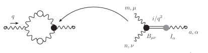
Figure 1: Pictorial representation of the Schwinger mechanism in SDE. White (black) circles denote fully dressed propagators (vertices); a gray circle attached to the external legs indicates that they are background gluons.

In this expression, the non perturbative quantity

$$B_{\mu\nu}(q,r,p)=B_{1}g_{\mu\nu}+B_{2}q_{\mu}q_{\nu}+B_{3}p_{\mu}p_{\nu}+B_{4}r_{\mu}q_{\nu}+B_{5}r_{\mu}p_{\nu},$$ (3)

is the effective vertex describing the interaction between the massless excitation and two gluons. $B_{\mu\nu}$ is to be identified with the “bound-state wave function” (or “BS wave function”) of the two-gluon bound-state, which, as we will see shortly, satisfies a homogeneous BSE. In addition, $i/q^{2}$ is the propagator of the scalar massless excitation. Finally, $\widetilde{I}_{\alpha}(q)$ is the (nonperturbative) transition amplitude, allowing the mixing between a (background) gluon and the massless excitation.

One can show [13] that, in the limit of zero momentum transfer $q^{2}=0$, the relevant quantity to consider is the form factor $B_{1}$ appearing in Eq. (3). Furthermore, due to Bose symmetry with respect to the interchange $\mu\leftrightarrow\nu$ and $p\leftrightarrow r$, we must have $B_{1}(q,r,p)=-B_{1}(q,p,r)$, which implies in the aforementioned kinematical limit that $B_{1}(0,-p,p)=0$. So, when $q\rightarrow 0$, what survives is the derivative $B_{1}^{\prime}$, which can be related to the derivative of the effective gluon mass through the exact all-order relation,

$$[m^{2}(p)]^{\prime}=-\widetilde{I}(0)B_{1}^{\prime}(p).$$ (4)

3 The Bethe-Salpeter equation

The existence of $B^{\prime}_{1}$ is of paramount importance for the mass generation mechanism; essentially, the question boils down to whether or not the dynamical formation of a massless bound-state excitation of the type postulated above is possible. As is well-known, in order to establish the existence of such a bound state one must (i) derive the appropriate BSE for the corresponding bound-state wave function, $B_{\mu\nu}$, (or, in this case, its derivative), and (ii) find non-trivial solutions for this integral equation. An approximate BSE for the bound-state wave function $B_{\mu\nu}$ is given by the following expression [see Fig. 2]

$$B_{\mu\nu}^{amn}=\int_{k}B_{\alpha\beta}^{abc}\Delta^{\alpha\rho}_{br}(k+q)\Delta^{\beta\sigma}_{cs}(k){\cal K}_{\sigma\nu\mu\rho}^{snmr}\,.$$ (5)

As explained in [13], Eq. (5) is obtained from the full BSE satisfied by the vertex $\widetilde{\Gamma}_{\alpha\mu\nu}$.

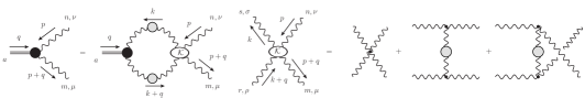
Figure 2: The BSE for the bound-state wave function $B_{\mu\nu}$ and the Feynman diagrams considered for the BS kernel.

We will next approximate the four-gluon BS kernel ${\cal K}$ by the lowest-order set of diagrams shown in Fig. 2, where the vertices are bare, while the internal gluon propagators are fully dressed. Going to Euclidean space, we define $x\equiv p^{2}$, $y\equiv k^{2}$, and $z\equiv(p+k)^{2}$; then, following the procedure outlined in [13], the BSE becomes

$$B^{\prime}_{1}(x) = -\frac{\alpha_{s}C_{A}}{12\pi^{2}}\int_{0}^{\infty}dyyB^{\prime}_{1}(y)\Delta^{2}(y)\sqrt{\frac{y}{x}}$$ (6)

$$\times \int_{0}^{\pi}d\theta\sin^{4}\theta\cos\theta\bigg{[}z+10(x+y)+\frac{1}{z}(x^{2}+y^{2}+10xy)\bigg{]}\Delta(z)\,.$$

As a further simplification, we approximate the gluon propagator $\Delta(z)$ appearing in the BSE of (6) [but not the $\Delta^{2}(y)$] by its tree level value, that is, $\Delta(z)=1/z$. Then, the angular integration may be carried out exactly, yielding

$$B^{\prime}_{1}(x) = \frac{\alpha_{s}C_{A}}{24\pi}\bigg{\{}\int_{0}^{x}dyB^{\prime}_{1}(y)\Delta^{2}(y)\frac{y^{2}}{x}\bigg{(}3+\frac{25}{4}\frac{y}{x}-\frac{3}{4}\frac{y^{2}}{x^{2}}\bigg{)}$$ (7)

$$+ \int_{x}^{\infty}dyB^{\prime}_{1}(y)\Delta^{2}(y)y\bigg{(}3+\frac{25}{4}\frac{x}{y}-\frac{3}{4}\frac{x^{2}}{y^{2}}\bigg{)}\bigg{\}}\,.$$

4 Numerical analysis

Next we discuss the numerical solutions for Eq. (7) for arbitrary values of $x$. Evidently, the main ingredient entering into its kernel is the nonperturbative gluon propagator, $\Delta(q)$. In order to explore the sensitivity of the solutions on the details of $\Delta(q)$, we will employ three infrared-finite forms focusing on their differences in the intermediate and asymptotic regions of momenta, given by

$$\Delta_{1}^{-1}(q^{2}) = q^{2}+m^{2}_{0}\,,$$ (8)

$$\Delta_{2}^{-1}(q^{2}) = q^{2}\left[1+\frac{13C_{\rm A}g^{2}}{96\pi^{2}}\ln\left(\frac{q^{2}+\rho\,m_{0}^{2}}{\mu^{2}}\right)\right]+m^{2}_{0}\,,$$ (9)

$$\Delta_{3}^{-1}(q^{2}) = m_{g}^{2}(q^{2})+q^{2}\left[1+\frac{13C_{\rm A}g_{1}^{2}}{96\pi^{2}}\ln\left(\frac{q^{2}+\rho_{1}\,m_{g}^{2}(q^{2})}{\mu^{2}}\right)\right].$$ (10)

The first expression (8) corresponds to a tree-level massive propagator, where $m^{2}_{0}$ is a hard mass treated as a free parameter. On the left panel of Fig. 3, the (blue) dotted curve represents $\Delta_{1}$ for $m_{0}=376\,\mbox{MeV}$. The second model (9) contains the renormalization-group logarithm next to the momentum $q^{2}$, where $\rho$ is an adjustable parameter varying in the range of $\rho\in[2,16]$. Notice that the hard mass $m_{0}^{2}$ appearing in the argument of the perturbative logarithm acts as an infrared cutoff. The (black) dashed line represents Eq. (9) when $\rho=16$, $m_{0}=376\,\mbox{MeV}$, and $\mu=4.3$ GeV. Finally, Eq. (10) is simply a physically motivated fit for the gluon propagator determined by the large-volume lattice simulations of Ref. [2], where $m^{2}_{g}(q^{2})=m^{4}/(q^{2}+\rho_{2}m^{2})$ is a a running mass. The values of the fitting parameters are $m=520$ MeV, $g_{1}^{2}=5.68$, $\rho_{1}=8.55$ and, $\rho_{2}=1.91$, and the (red) continuous line on the left panel of Fig. 3 represents this propagator. Notice that, in all three cases, we have fixed the value of $\Delta^{-1}(0)=m_{0}^{2}\approx 0.14$.

Our main findings may be summarized as follows.

(a) In Fig. 3, right panel, we show the solutions of Eq. (7) obtained using as input the three propagators shown on the left panel. For the simple massive propagator of Eq. (8), a solution for $B^{\prime}_{1}$ is found for $\alpha_{s}=1.48$; in the case of $\Delta_{2}$ given by Eq. (9), a solution is obtained when $\alpha_{s}=0.667$, while for the lattice propagator $\Delta_{3}$ of Eq. (10) a non-trivial solution is found when $\alpha_{s}=0.492$.

(b) Note that, due to the fact that Eq. (7) is homogeneous and (effectively) linear, if $B^{\prime}_{1}$ is a solution then the function $cB^{\prime}_{1}$ is also a solution, for any real constant $c$. Therefore, the solutions shown on the right panel of Fig. 3 corresponds to a representative case of a family of possible solutions, where the constant $c$ was chosen such that $B^{\prime}_{1}(0)=1$.

(c) Another interesting feature of the solutions of Eq. (7) is the dependence of the observed peak on the support of the gluon propagator in the intermediate region of momenta. Specifically, an increase of the support of the gluon propagator in the approximate range (0.3-1) GeV results in a more pronounced peak in $B^{\prime}_{1}$.

(d) In addition, observe that due to the presence of the perturbative logarithm in the expression for $\Delta_{2}$ and $\Delta_{3}$, the corresponding solutions $B^{\prime}_{1}$ fall off in the ultraviolet region much faster than those obtained using the simple $\Delta_{1}$ of Eq. (8).

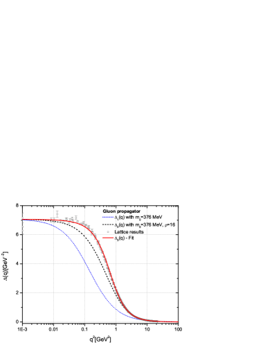
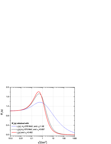
Figure 3: The three models for the gluon propagator (left) and the corresponding solutions of the BS equation for $B^{\prime}_{1}(x)$ (right).

5 Conclusions

In this presentation we have reported recent progress [13] on the study of the Schwinger mechanism in QCD, which endows gluons with a dynamical mass in a gauge invariant way. This mechanism relies on the existence of massless bound-state excitations, whose dynamical formation is controlled by a homogeneous BSE. As we have seen, under certain simplifying assumptions, this equation admits non-trivial solutions, thus furnishing additional support in favor of the specific mass generation mechanism described in a series of earlier works [6, 7, 8]. In the future, this framework may serve as a starting point towards a consistent first-principle treatment of glueballs as bound states of gluons, at nonvanishing momenta. Specifically, one may envisage a combined BS and SDE analysis, in the spirit of similar approaches in the case of color singlets $q\bar{q}$ bound states, employed in the literature for the dynamical description of mesons.

Acknowledgments:

This research is supported by the European FEDER and Spanish MICINN under grant FPA2008-02878.

References

- [1] A. Cucchieri and T. Mendes, Phys. Rev. D 81, 016005 (2010).
- [2] I. L. Bogolubsky, E. M. Ilgenfritz, M. Muller-Preussker and A. Sternbeck, PoS LATTICE, 290 (2007) ; Phys. Lett. B 676, 69 (2009).
- [3] P. O. Bowman et al., Phys. Rev. D 76, 094505 (2007).
- [4] O. Oliveira and P. J. Silva, PoS LAT2009, 226 (2009).
- [5] J. M. Cornwall, Phys. Rev. D 26, 1453 (1982).
- [6] A. C. Aguilar and J. Papavassiliou, JHEP 0612, 012 (2006).
- [7] A. C. Aguilar, D. Binosi and J. Papavassiliou, Phys. Rev. D 78, 025010 (2008).
- [8] A. C. Aguilar, D. Binosi and J. Papavassiliou, Phys. Rev. D 84, 085026 (2011)
- [9] J. S. Schwinger, Phys. Rev. 125, 397 (1962).
- [10] R. Jackiw and K. Johnson, Phys. Rev. D 8, 2386 (1973).
- [11] E. Eichten and F. Feinberg, Phys. Rev. D 10, 3254 (1974).
- [12] O. Oliveira and P. Bicudo, J. Phys. G 38, 045003 (2011).
- [13] A. C. Aguilar, D. Ibanez, V. Mathieu and J. Papavassiliou, Phys. Rev. D 85 (2012) 014018 .
- [14] D. Binosi and J. Papavassiliou, Phys. Rept. 479, 1-152 (2009).