Growth, competition and cooperation in spatial population genetics

Abstract

We study an individual based model describing competition in space between two different alleles. Although the model is similar in spirit to classic models of spatial population genetics such as the stepping stone model, here however space is continuous and the total density of competing individuals fluctuates due to demographic stochasticity. By means of analytics and numerical simulations, we study the behavior of fixation probabilities, fixation times, and heterozygosity, in a neutral setting and in cases where the two species can compete or cooperate. By concluding with examples in which individuals are transported by fluid flows, we argue that this model is a natural choice to describe competition in marine environments.

1 Introduction

A mathematical analysis of the fate of mutations in spatially extended populations has been a classic topic of research in population genetics for at least seventy years (Fisher, 1937; Kolmogorov et al., 1937; Wright, 1943; Kimura, 1953; Kimura and Weiss, 1964). This interest has nevertheless increased recently, as improved sequencing technology allows direct observations of structured genetic diversity in space for many different species.

On the theoretical side, a landmark in this research has been the stepping stone model (SSM) proposed by Kimura (Kimura, 1953; Kimura and Weiss, 1964). This model considers $m$ islands (or “demes”), each having a fixed local population size $N_{l}$ and arranged along a line or in a regular lattice in more than one spatial dimension. The population on each island is made up of several species (or alleles) described by, e.g., a Wright-Fisher or Moran process. Spatial migration is modeled by assuming that neighboring islands exchange individuals at some given rate.

It is often convenient to describe the state of the system in terms of the macroscopic density of individuals $f(\mathbf{x},t)$ carrying one of the two alleles. In the continuum limit, the macroscopic equation governing the time evolution of such density reads

$$\partial_{t}f(\mathbf{x},t)=D\nabla^{2}f(\mathbf{x},t)+sf(1-f)+\sqrt{\frac{f(1-f)}{N}}\xi(\mathbf{x},t)$$ (1)

where $N=N_{l}/a^{d}$, $a$ is the lattice spacing between two neighboring islands, $d$ the spatial dimension, and $\xi(\mathbf{x},t)$ is a Gaussian stochastic process, delta correlated in space and time, $\langle\xi(\mathbf{x},t)\xi(\mathbf{x}^{\prime},t^{\prime})\rangle=\delta(\mathbf{x}-\mathbf{x}^{\prime})\delta(t-t^{\prime})$. Here, $f=1$ means an island exclusively populated with one allele and $f=0$ means exclusive occupation by the alternative genotype. The nonlinearity multiplying the noise requires an interpretation in terms of the Ito calculus (Korolev et al., 2009).

However, in many realistic cases, the mechanism of species movement and range expansion is more complicated than a simple diffusion process. For example, recent observations on crabs colonies along the east coast of north America (Pringle et al., 2011) demonstrated how invasion of one allele is controlled by the asymmetrical advection of larvae from north to south by a coastal current. The interplay between population genetics and individual movement (and transport) can be even more complex in the open ocean, where individuals belonging to different planktonic and bacterial species are stirred and mixed by chaotic flows (Tel et al., 2005; Neufeld and Hernandez-Garcia, 2009; D’Ovidio et al., 2010; Perlekar et al., 2010; Benzi et al., 2012). Of particular interest is the population genetics of photosynthetic organisms that control their buoyancy to remain near the surface of an aquatic environment. In this case, the advecting flows are effectively compressible, leading to population densities that overshoot the normal carrying capacity (Perlekar et al., 2010; Pigolotti et al., 2012).

While the SSM can be generalized to include a constant asymmetric diffusion (see i.e. (Pringle et al., 2011)), the extension to more complex fluid environments is more subtle. One of the main underlying assumptions of the SSM – a local population size that does not vary either in time nor in space – is quickly violated in aquatic environments where flows create inhomogeneities in the total density of individuals. Individual-based competition models without strict population size conservation have already been studied, for example allowing for the possibility of empty sites (Neuhauser, 1991; O’Malley et al., 2006b, a; spatial competition under a reproduction–mortality constraint, 2009; Cencini et al., 2012). However, when flows are introduced, it is also less appropriate to discretize the system in space into demes with a fixed size. In compressible turbulence, for example, the density of individuals can be inhomogeneous on a wide variety of spatial scales (Perlekar et al., 2010), even inside a single deme (which in the SSM is assumed to be well-mixed).

In this paper, with the goal of describing population genetics in aquatic environments in mind, we introduce a new model in which individuals carrying two different alleles $A$ and $B$ live in a continuous space. Their individual densities are allowed to grow and fluctuate, including the important possibility of overshooting the natural carrying capacity. Indeed, note that naively assuming compressible flows that make $f>1$ would lead to an imaginary noise amplitude in Eq. (1)! The model we study is similar in spirit to the stochastic logistic equation (Law et al., 2003; Hernandez-Garcia and Lopez, 2004; Birch and Young, 2006). However, in this study we focus on competition and cooperation of two species, rather than the stochastic growth of a single population. The second difference is that previous studies focused on patterns formed by the non-local nature of competition (Hernandez-Garcia and Lopez, 2004; Birch and Young, 2006). In this paper, we mostly focus on the parameter range in which such patterns are not formed and a weak noise description in the spirit of Eq. (1) is appropriate.

The phenomenology of such a model, even in the presence of very simple flows, is very rich due to the interplay between population dynamics and fluid advection (see Pigolotti et al. (2012) for some of the consequences in one dimension). For this reason, we devote a large portion of this work to the case in which the flow is absent and individuals move in space in a diffusive way. This simple case allows for a systematic comparison with the known results of the SSM. In particular, we show that there exists a parameter range where the predictions of our model are consistent with Eq. (1) and its generalization to include competitive exclusion and mutualism (Korolev and Nelson, 2011). In simple cases, such as when the two species are neutral variants of each other, this correspondence can be shown analytically. In more complex cases, the correspondence is explored by means of numerical simulations. The last part of the work discusses an example in which a compressible flow transport the individuals, as an example of a problem that cannot be treated within the context of the SSM.

In Sec. 2, we sketch the model of growth, competition and cooperation studied here, which leads to the two-species model for allele densities $c_{A}(\mathbf{x},t)$ and $c_{B}(\mathbf{x},t)$ summarized in Eq. (2). We focus on three interesting cases: (1) strictly neutral competitions, (2) a reproductive advantage of one species over the other and (3) mutualistic situations where cooperation plays a role. Sec. 3 discusses the behavior of our model in the “zero-dimensional” well-mixed case in which the population is not structured in space, which allows us to determine limits such that standard Wright-Fisher and Moran results for population genetics can be recovered from our more general model. We then explore in Sec. 4 the long-time behavior of our model without fluid advection in one and two spatial dimensions. Examples of the behavior of the model in the presence of fluid advection are discussed in Sec. 5. Concluding remarks are presented in Sec. 6. A detailed derivation of our model equation is contained in Appendix A. Appendix B shows how conventional stepping stone model results can be recovered in certain limits. Appendix C describes a limit in which a mutualistic generalization of the famous Kimura formula for fixation probabilities (Crow and Kimura, 1970) is possible.

2 Model

Many widely studied models of population genetics in space, the most notable example being the stepping stone model, consider individuals carrying different alleles that occupy sites (also called “demes”) on a lattice. It is commonly assumed that each site is always saturated up to its carrying capacity, so that, at each deme, the local population size $N_{l}$ is constant during the dynamics.

We relax these assumptions by considering discrete individuals $X_{i}$ carrying different alleles (denoted by the index $i$) and diffusing in continuous space (with a diffusion constant $D$, for simplicity equal for all individuals). Further, we implement population dynamics assuming that individuals carrying allele $i$ reproduce at rate $\mu_{i}$ and die with rates $\tilde{\lambda}_{ij}$ proportional to the number of individuals carrying a (possibly) different allele $j$ in a region of spatial size $\delta$ centered on their position. For example, in one dimension ($1d$), $\delta$ will be an interaction length, while in $2d$ it will be an interaction area. In a language borrowed from chemical kinetics, the “reactions” we consider are:

$$X_{i} \stackrel{{\scriptstyle\mu_{i}}}{{\rightarrow}} 2X_{i}\qquad\mathrm{(reproduction)}$$

$$X_{i}+X_{j} \stackrel{{\scriptstyle\tilde{\lambda}_{ij}}}{{\rightarrow}} X_{i}\qquad\mathrm{(death}\ \mathrm{by}\ \mathrm{competition)}$$ (2)

In the case of a single species, this set of reactions is commonly referred to as the birth-coagulation process (Doering et al., 2003). In this paper, we will focus on the case of two alleles, $i=A,B$. Other reactions could be added to the ones above, for example the possibility that an individual can die even in absence of competition, $X_{i}\rightarrow\emptyset$, or reactions implementing more complex biological interactions. We will limit ourselves to the biological dynamics embodied in (2), which contains minimal ingredients necessary to generate most of the main features present in more complicated models. Notice that, in contrast to models such as the Moran process, the density of individuals is not fixed but fluctuates both locally and globally.

In order to make the presentation more compact, we start by discussing the spatially explicit version of the model and then discuss the globally well-mixed version as a limiting case. We consider the number densities $n_{A}(\mathbf{x},t)$ and $n_{B}(\mathbf{x},t)$, that integrated over a region of space yield the (stochastic) number of individuals of species $A$ or $B$ in that region. We will study cases in which the number densities are typically large, and consequently define concentrations $c_{A}(\mathbf{x},t)=n_{A}(\mathbf{x},t)/N$ and $c_{B}(\mathbf{x},t)=n_{B}(\mathbf{x},t)/N$ via a constant parameter $N$, assumed to be of the same order of magnitude of $n_{A}$ and $n_{B}$. This means that, by definition, a constant density $c=1$ corresponds to a uniform distribution of $N$ individuals in a segment of length $1$ in one dimension. More generally, in $d$ dimensions, a concentration $c(\mathbf{x},t)=1$ will correspond to a total number of particles $\mathcal{N}=NL^{d}$ in a system of linear size $L$. With this choice, the macroscopic equations describing the dynamics of the concentrations $c_{A}$, $c_{B}$ of species $A$ and $B$ read:

$$\frac{\partial}{\partial t}c_{A} = D\nabla^{2}c_{A}+c_{A}(\mu_{A}-\lambda_{AA}c_{A}-\lambda_{AB}c_{B})+\sqrt{\frac{c_{A}(\mu_{A}+\lambda_{AA}c_{A}+\lambda_{AB}c_{B})}{N}}\xi$$

$$\frac{\partial}{\partial t}c_{B} = D\nabla^{2}c_{B}+c_{B}(\mu_{B}-\lambda_{BA}c_{A}-\lambda_{BB}c_{B})+\sqrt{\frac{c_{B}(\mu_{B}+\lambda_{BA}c_{A}+\lambda_{BB}c_{B})}{N}}\xi^{\prime}$$ (3)

where $\xi(\mathbf{x},t)$ and $\xi^{\prime}(\mathbf{x},t)$ are independent Gaussian random variables, delta-correlated in space and time, $<\xi(\mathbf{x},t)\xi(\mathbf{x},t^{\prime})>=\delta(t-t^{\prime})\delta(\mathbf{x}-\mathbf{x}^{\prime})$ that should be interpreted according to the Ito prescription (Korolev et al., 2009). The macroscopic binary reaction rates $\lambda_{ij}$ multiplying the quadratic terms in the concentrations are defined in terms of the microscopic binary rates $\tilde{\lambda}_{ij}$ as $\lambda_{ij}=N\delta\tilde{\lambda}_{ij}$, where $\delta$ is the interaction domain defined above. In the following, we will focus on cases in which the $\mu_{i}$’s and the $\lambda_{ij}$’s are of the same order of magnitude, so that typical values of the total concentration $c_{A}+c_{B}$ are order $1$. Under these assumptions, it is useful to note that the quantity $2N^{-1}=2\delta/(\tilde{\lambda}_{ij}/\lambda_{ij})$ plays here the same role of the genetic diffusion constant in the stepping stone model. In particular, $\delta$ is analogous of the lattice spacing, while the denominator on the right hand side can be thought as the carrying capacity of each deme. A detailed derivation of Eqs. (2), together with a discussion of its limits of validity, is presented in Appendix A. If the species densities are well-mixed and we neglect stochastic number fluctuations, the deterministic dynamics embodied in Eqs. (2) is a familiar model of growth, selection and competition in asexual populations (Smith, 1998). The four different types of dynamics that emerge depending on the values of the $\lambda_{ij}$’s are reviewed at the end of this section. Our aim here is to understand the rich behaviors possible when both spatial variations and number fluctuations are allowed.

To limit the parameter space, we will consider the following three biologically relevant choices for the reaction rates:

1. Neutral Theory

   This choice is appropriate when the two biological species (or strains, or mutants and wild type alleles) are neutral variants of each other. This means that their growth rates and carrying capacities are the same; further, competition with an individual belonging to the same species is the same as competition with an individual of the other species. In formulas, for Eq. (2), a convenient neutral parameter choice is: $\mu_{A}=\mu_{B}=\lambda_{AA}=\lambda_{AB}=\lambda_{BA}=\lambda_{BB}=\mu$.

2. Reproductive advantage

   In this setting, we depart from neutrality by allowing for a different reproduction rate of species $A$: $\mu_{A}=\mu(1+s)$ while all the other rates (including the $\lambda_{ij}$) are equal to $\mu$ as in the neutral case. We will study this case to explore the effect of a selective advantage of one of the two species on the dynamics of the model. In particular, $s>0$ implies a selective advantage for $A$ and $s<0$ is a disadvantage. Clearly, neutrality is recovered for $s=0$.

3. Mutualistic setting

   A simple way to study mutualistic interactions is to assume that the only departure from neutrality occurs in the intensity of competition between individuals carrying different alleles. In formulas, we have $\mu_{A}=\mu_{B}=\mu$, $\lambda_{AA}=\mu$, $\lambda_{BB}=\mu$, $\lambda_{AB}=\mu(1-\epsilon_{A})$, and $\lambda_{BA}=\mu(1-\epsilon_{B})$. The corresponding macroscopic equations are well defined only for $\epsilon_{A},\epsilon_{B}\leq 1$, so that the competition rates $\lambda_{ij}$ are non-negative. We will focus mostly on the case $\epsilon_{A}>0$ and $\epsilon_{B}>0$. In this regime, spatial number fluctuations play an important role (Korolev and Nelson, 2011) and competition between species is reduced (we will interpret this reduction as the effect of mutualistic interactions). Other choice could also be of interest, for example $\epsilon_{A}=0$ and $\epsilon_{B}<0$ is another way of allowing a competitive advantage of $A$ over $B$ (in this case, via enhanced competition rather than via a larger reproduction rate). We note finally that $\epsilon_{A}<0$, $\epsilon_{B}<0$ corresponds to a competitive exclusion model, arising for example when the competing variants secret toxins that inhibit the growth of their competitors.

In the following, we will measure time in units of a generation time so that $\mu=1$. A convenient choice of the interaction domain is of the order of the average spacing among individuals, $\delta=1/N$, so that $\lambda_{ij}=\tilde{\lambda}_{ij}$. This choice also implies $N_{l}=1$. For simplicity, we will present most of the spatial results for the one-dimensional version of the model, introducing two-dimensional results only as appropriate. In the spatially explicit case, the system is a segment of length $L$ with periodic boundary conditions. We will present also two dimensional simulations, where the system is a $L\times L$ square, also with periodic boundary conditions.

An even simpler setting we will study to make contact with traditional Moran or Fisher-Wright models is the case in which the population can be assumed to be well-mixed, or “zero-dimensional”. This limiting case can be easily obtained from the one dimensional case by setting $\delta=L=1$ and ignoring spatial diffusion, since each individual now interacts with every other individual in the population. As a consequence of this choice, one now has $N=\lambda_{ij}/\tilde{\lambda}_{ij}$. In this case, the spatial position of the individuals is irrelevant for biological interactions. Clearly, in this special case, the individual density is equivalent to the total number of individuals $N\equiv N_{l}\equiv\mathcal{N}$.

Both in the spatial and well-mixed cases, we will compare analytical predictions obtained from the continuum theory of Eqs. (2) with simulations of the individual-based dynamics encoded in the reactions of Eqs. (2). Details on the numerical scheme implemented for the individual-based model are in Appendix A and in (Perlekar et al., 2011).

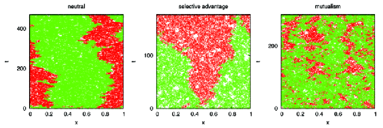
Figure 1: Three illustrative parameters choices in the one dimensional version of the model. In all panels $D=10^{-4}$ and $N=100$. The left panel corresponds to the neutral choice in which all rates are set to one and initially the two species are randomly distributed with equal concentrations. In the center panel, all parameters are set to one except the reproduction rate of allele $A$ (in red) which reproduces at a rate $(1+s)$ with a large selective advantage $s=0.3$; in this case, the initial fraction of $A$ is $0.1$. In the right panel, competition among species is reduced by taking $\epsilon_{A}=\epsilon_{B}=0.7$ to enhance mutualism; in this case the two species are randomly distributed with equal concentrations in the initial condition. In this case, mutualism insures that the species (or alleles) remain spatially inhomogeneous out to very long times.

In Fig. (1), we anticipate some of the results to illustrate the qualitative behaviors that can be explored with the three aforementioned parameter choices in one spatial dimension. In the left panel, the two alleles are neutral. Despite fluctuation of the total density, the phenomenology is similar to that of the $1d$ stepping stone model: as time progresses, the two alleles are demixed and fixation occurs by coalescence of the domain boundaries, which can be regarded as annihilating random walks. In the central panel, species $A$ (in red) initially constitutes only $10\%$ of the total population; however, it has a reproductive advantage over species $B$. Despite the discreteness of individuals and density fluctuations, there are two noisy Fisher waves by which the initial minority can take over the entire population. Finally, in the right panel we simulate a case in which mixing of the two species is promoted by reducing competition among different alleles. In this case, we expect the two species to remain mixed indefinitely in the limit of large system size.

In the remainder of this section, we introduce some of the concepts we want to investigate in the simple case of a well mixed system without number fluctuations. Intuition about mutualistic behavior (and its opposite, competitive exclusion (Frey, 2010)) can be obtained by neglecting both the spatial degrees of freedom and the noise terms in Eq. (2). In this simple case, the dynamics reduces to (Korolev et al., 2012)

$$\frac{d}{dt}n_{A}(t)=n_{A}(t)\left[\mu_{A}-\tilde{\lambda}_{AA}n_{A}(t)-\tilde{\lambda}_{AB}n_{B}(t)\right]$$

$$\frac{d}{dt}n_{B}(t)=n_{B}(t)\left[\mu_{B}-\tilde{\lambda}_{BA}n_{A}(t)-\tilde{\lambda}_{BB}n_{B}(t)\right].$$ (4)

Note that the intrinsic carrying capacities (i.e., the steady state densities of one species when the other is absent) for this model are $N_{A}=\mu_{A}/\tilde{\lambda}_{AA}$ and $\qquad N_{B}=\mu_{B}/\tilde{\lambda}_{BB}$. These quantities (we always choose parameters such that $N_{A}\approx N_{B}$) play the role of the parameter $N$ that controls stochastic number fluctuations in the general case of Eq. (2). As mentioned above for case 3, an especially interesting situation arises when (1) the two species grow at identical rates when the numbers are dilute, so that $\mu_{A}=\mu_{B}=\mu$; (2) also the self-competition terms are also identical, $\tilde{\lambda}_{AA}=\tilde{\lambda}_{BB}$; and (3) the effect of cooperation or competitive exclusion is contained exclusively in the cross-interactions, $\tilde{\lambda}_{AB}\equiv\tilde{\lambda}_{AA}(1-\epsilon_{A})$ and $\lambda_{BA}\equiv\tilde{\lambda}_{BB}(1-\epsilon_{B})$. With this choice, and rescaling the time unit by a factor $\mu^{-1}$, the equations for the concentrations $c_{A}=n_{A}/N_{A}$ and $c_{B}=n_{B}/n_{B}$ corresponding to system (2) read

$$\frac{d}{dt}c_{A}=c_{A}\left[1-c_{A}-c_{B}+\epsilon_{A}c_{B}\right]$$

$$\frac{d}{dt}c_{B}=c_{B}\left[1-c_{A}-c_{B}+\epsilon_{B}c_{A}\right].$$ (5)

The remaining two parameters $\epsilon_{A}$ and $\epsilon_{B}$ control the competition under “crowded conditions”, such that the populations have grown up to satisfy $c_{A}+c_{B}\approx 1$. If the two variants are nearly identical, it is reasonable to assume $|\epsilon_{A}|$, $|\epsilon_{B}|\ll 1$. As illustrated in Fig. 2, the deterministic system (2) always has fixed points at $(0,0)$, $(0,1)$, and $(1,0)$. Depending on the parameters, there can also be a fourth fixed point (Smith, 1998) located at

$$(c_{A}^{*},c_{B}^{*})=\frac{(\epsilon_{A},\epsilon_{B})}{\epsilon_{A}+\epsilon_{B}-\epsilon_{A}\epsilon_{B}}.$$ (6)

When cooperation is favored ($\epsilon_{A},\epsilon_{B}>0$, Fig. 2a) this fixed point is stable, and leads to a steady state population fraction $f^{*}$ of $A$ individuals, $0<f^{*}<1$, with

$$f^{*}\equiv\frac{c_{A}^{*}}{c_{A}^{*}+c_{B}^{*}}=\frac{\epsilon_{A}}{\epsilon_{A}+\epsilon_{B}}.$$ (7)

When competitive exclusion (Frey, 2010) is favored ($\epsilon_{A},\epsilon_{B}<0$, fig. 2b) this fixed point is unstable to the attracting fixed points $(1,0)$ or $(0,1)$, depending on the initial conditions. Genetic demixing, present in strictly neutral systems only due to stochastic number fluctuations, is enhanced in this case. Finally, when $\epsilon_{A}$ and $\epsilon_{B}$ have opposite signs, the fixed point (6) lies outside the biologically relevant domain, and one of the two fixed points $(1,0)$ or $(0,1)$ becomes globally stable, corresponding to a competitive advantage for one species or the other when the population is dense.

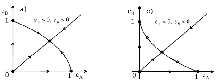
Figure 2: Deterministic dynamics of the mutualistic model in zero dimensions without number fluctuations. In a), the interactions $\epsilon_{A}>0$ and $\epsilon_{B}>0$ favor cooperation, and there is a stable fixed point $(c_{A}^{*},c_{B}^{*})$ with both densities nonzero. In B), the organisms secrete toxins that impede each others growth, so $\epsilon_{A}<0$ and $\epsilon_{B}<0$ and the fixed point $(c_{A}^{*},c_{B}^{*})$ is unstable.

Suppose we now introduce spatial migration and number fluctuations, to recover the full model defined by Eq. (2). When might we expect fixation probabilities, the global heterozygosity, correlation functions etc. to reduce to the familiar results for conventional spatial stepping stone-type models with strictly conserved population sizes in every deme? A particularly simple case, corresponding to the selectively neutral limit $\epsilon_{A}=\epsilon_{B}=0$, is illustrated for a well-mixed system in Fig. 3a below: the population grows up and eventually wanders along the line $c_{A}+c_{B}=1$, until it reaches the absorbing states at $(1,0)$ or $(0,1)$. A more general situation is $\epsilon_{A}+\epsilon_{B}=0$, in which case one variant typically has a simple selective advantage along an invariant subspace given by the line $c_{A}+c_{B}=1$. If the fluctuations transverse to this line are small (corresponding to a large population size), then the usual formulas for fixation probabilities hold, as we show later in this paper. In more general situations, however, it is no longer exactly true that the population localizes at long times near the straight line $c_{A}+c_{B}=1$. Indeed, we have from Eq. (6) that

$$c_{A}^{*}+c_{B}^{*}=\frac{\epsilon_{A}+\epsilon_{B}}{\epsilon_{A}+\epsilon_{B}-\epsilon_{A}\epsilon_{B}},$$ (8)

which exceeds 1 along the outwardly bowed incoming trajectories in Fig. 2a, and is less than $1$ for the outgoing inwardly curved trajectory in Fig. 2b. However, we do have the approximate equality, $c^{*}_{A}+c^{*}_{B}\approx 1$, provided $|\epsilon_{A}+\epsilon_{B}|\ll|\epsilon_{A}\epsilon_{B}|$ in Eq. (8). In this limit, a combination of numerical and analytic arguments presented in this paper show that formulas recently derived for mutualistic and competitive exclusion stepping stone models (Korolev and Nelson, 2011) apply to the current model with demographic fluctuations as well, again provided that the overall population size $N$ is sufficiently large.

What happens if $\mu_{A}$ and $\mu_{B}$ are unequal, but $\epsilon_{A}$ and $\epsilon_{B}$ remain small? In this case, the population proportions will certainly change as an initially small population like that in Fig. 3a grows to approach the line $c_{A}+c_{B}\approx 1$. However, once this line is reached, the subsequent time evolution should again be given by stepping stone model results.

3 Well-mixed case with number fluctuations

In this section, we present the results in the simple well-mixed (or “zero-dimensional”) version of the model. Thus, we keep number fluctuations in Eq. (2), but neglect spatial variations in the allele concentrations.

3.1 Neutral theory

As previously discussed, it is useful to describe the dynamics of the neutral version of the model in the $c_{A}$ vs. $c_{B}$ plane, as depicted in Fig. (3, left). Starting from a dilute initial condition, the system evolves rapidly towards to the intrinsic overall carrying capacity given by $c_{A}+c_{B}=1$. The dynamics is then localized near this line (with fluctuations), until one of the two species goes extinct. This behavior contrasts with the Moran process in which the dynamics is rigidly confined to the $c_{A}+c_{B}=1$ line, since no fluctuations of the total density are allowed. To determine when these fluctuations are small, first note from Eq. (2) that in the neutral case the total concentration $c_{T}=c_{A}+c_{B}$ obeys a closed equation:

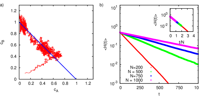
Figure 3: Neutral dynamics in the well-mixed case. (a) Example of a trajectory in the $(c_{A},c_{B})$ plane with $N=500$. The initial condition is $n_{A}=n_{B}=20$, i.e. a small fraction of a typical long time carrying capacity. (b) Decay of the average heterozygosity $\langle H(t)\rangle$ for different values of $N$. Curves are obtained from simulations of the particle model; each curve is an average over $10^{4}$ realizations and the error bars are smaller than the size of the lines. (inset) Same curves plotted as a function of $t/N$. Note the data collapse.

$$\frac{d}{dt}c_{T}=\mu c_{T}(1-c_{T})+\sqrt{\frac{\mu c_{T}(1+c_{T})}{N}}\xi_{c},$$ (9)

decoupled from the fraction of species $A$, $f=c_{A}/(c_{A}+c_{B})$, where the noise term $\xi_{c}$ satisfies $\langle\xi_{c}(t)\xi_{c}(t^{\prime})\rangle=\delta(t-t^{\prime})$. When $N$ is large, the stationary solution, beside the solution $P(c)=\delta(c)$ corresponding to global extinction that will eventually be reached on long times of order $\exp(N)$, is approximately a Gaussian with average $\langle c_{T}\rangle=1$ and variance $\langle c_{T}^{2}\rangle-\langle c_{T}\rangle^{2}=N^{-1}$, which is small when $N$ is large.

We now describe the dynamics of the relative fraction $f$ of individuals carrying allele $A$, $f=c_{A}/(c_{A}+c_{B})$. The equation for $f(t)$, derived in B, reads

$$\frac{d}{dt}f=\sqrt{\mu f(1-f)\frac{1+c_{T}}{Nc_{T}}}\xi_{f}.$$ (10)

where $\xi_{f}(t)$ also satisfies $\langle\xi_{f}(t)\xi_{f}(t^{\prime})\rangle=\delta(t-t^{\prime})$, and further we have $\langle\xi_{f}(t)\xi_{c}(t^{\prime})\rangle=0$. The above equation allows us to analyze the global heterozygosity, which quantifies the loss of diversity as time evolves and is defined as the probability $H(t)=2\langle f(1-f)\rangle$ that two randomly chosen individuals in the population carry different alleles.

As mentioned above, the equation for $c_{T}$ is independent of $f$ in the neutral case studied here. As a result, one can factorize the average over $c_{T}$ and $f$ in the equation for $H(t)$:

$$\frac{d}{dt}H(t)=-\frac{\mu}{N}\left\langle f(1-f)\frac{1+c_{T}}{c_{T}}\right\rangle=-\frac{\mu}{N}\left\langle f(1-f)\right\rangle\left\langle\frac{1+c_{T}}{c_{T}}\right\rangle=-\frac{2\mu}{N}H(t)+O\left(\frac{1}{N^{2}}\right).$$ (11)

Neglecting the correction of order $N^{-2}$, we recover for our model with density fluctuations the closed equation for $H(t)$ for Fisher-Wright and Moran-type models with a fixed population size derived by Kimura, which states that the total heterozygosity decays exponentially in well mixed neutral systems (Crow and Kimura, 1970):

$$\langle H(t)\rangle=H(0)\exp(-2\mu t/N)$$ (12)

Fig. (3b) confirms this exponential behavior in simulations of the model.

3.2 Reproductive advantage

In a well-mixed finite population and in absence of mutations, diversity will be lost and only one of the two alleles will survive after a long enough time. We now study the probability of allele $A$ to fixate in a well-mixed population of size $N\gg 1$, in the case in which the allele confers a small reproductive advantage $s\ll 1$. In the same spirit as the previous section, we can derive the equation for the relative fraction $f=c_{A}/(c_{A}+c_{B})$ (see B). Upon neglecting terms proportional to $s/N$, the equation in this case reads:

$$\frac{d}{dt}f=\mu sf(1-f)+\sqrt{\mu f(1-f)\frac{1+c_{T}}{Nc_{T}}}\xi$$ (13)

As in Eq. 10, this result must be supplemented with the equation for the total concentration $c_{T}=c_{A}+c_{B}$. Although in the non-neutral case the equation for $c_{T}$ is no longer independent of $f$, one can show that the averages over $c_{T}$ and $f$ factorize up to terms of order $s/N$ or higher that can be safely neglected for $s\ll 1$ and $N\gg 1$.

These observations allows us to recover the formula for the probability of fixation of allele $A$ (Crow and Kimura, 1970).

$$p_{fix}=\frac{1-e^{-sNf_{0}}}{1-e^{-sN}}$$ (14)

where $f_{0}$ is the fraction of individuals carrying allele $A$ once trajectories like that in Fig (3a) reach the line $c_{A}+c_{B}=1$. This result is again similar to Fisher-Wright or Moran models with a strictly fixed total population size. Eq. (14) is tested with simulations in Fig. 4.

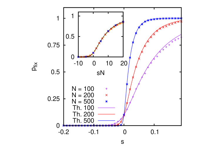
Figure 4: Fixation in the well-mixed case with reproductive advantage. Probability of fixation for different values of $s$ and $N$ (listed in the figure) for the well-mixed version of the particle model, compared with the prediction of Eq. (14). The initial fraction of individuals belonging to species $A$ is $f_{0}=0.1$, with $c_{T}=1$ initially. The inset shows that all curves collapse when plotted as a function of $sN$. These curves are again averages over $10^{4}$ independent realizations.

3.3 Mutualism

In the well-mixed limit of the mutualistic model, fixation always occurs at $(c_{A},c_{B})=(1,0)$ or $(0,1)$ after a long enough time. However, when the total number of individuals is large, this time grows exponentially with $N$ and can easily become inaccessible to experiments (and simulations). As detailed in C, the quasi-stationary solution where the two cooperating species coexist for $\epsilon_{A},\epsilon_{B}>0$ can be seen as a state confined by two potential barriers, one inhibiting species $A$ to fixate and the other inhibiting species $B$ to fixate. When $N$ is large, it will be extremely probable that fixation will occur by passing the lowest of these two barriers. In this case, an estimate of the time $t^{*}$ needed to reach fixation can be derived by calculating the height of the lowest barrier and applying Kramer’s escape rate theory. The result is:

$$t^{*}\sim\exp\left[\frac{N}{2}\frac{\min(\epsilon_{A}^{2},\epsilon_{B}^{2})}{\epsilon_{A}+\epsilon_{B}}\right].$$ (15)

Figure (5) shows a heat map of the total heterozygosity in the ($\epsilon_{A},\epsilon_{B}$ plane for $N=500$ after $5000$ generations. The black region is where fixation occurred. Green lines are the theoretical limits of the apparent coexistence region obtained from Eq. 15.

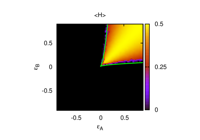
Figure 5: Finite-time coexistence in the well-mixed mutualistic model. Average heterozygosity in the $(\epsilon_{A},\epsilon_{B})$ plane, with $N=500$, in $d=0$ dimensions, i.e. for the well-mixed model. Simulations are run until a time $t=5000$. For each pair of $(\epsilon_{A},\epsilon_{B})$ values, after a transient, the heterozygosity approaches a quasi-stationary value. The green line limits the region in which coexistence up to this time is possible according to the estimate (15).

After estimating the fixation time in the mutualistic model, we now ask: what is the fixation probability of one of the two alleles? In Appendix C, we show that in the appropriate limit the fixation probability for mutualists obeys a formula similar to the result for a stepping stone model with fixed total population size (Korolev and Nelson, 2011), namely

$$u(f_{0})=\frac{\int_{0}^{f_{0}}e^{\frac{1}{2}Ns(f^{*}-p)^{2}}}{\int_{0}^{1}e^{\frac{1}{2}Ns(f^{*}-p)^{2}}},$$ (16)

where $f_{0}$ is the initial fraction of allele $A$. In the limit $f^{*}\rightarrow\infty$, $s\rightarrow 0$, with a mutualistic effective selective advantage $\tilde{s}=f^{*}s$ fixed, this reduces to the famous Kimura formula discussed above

$$u(f_{0})~{}=~{}\frac{1-e^{-N\tilde{s}f_{0}}}{1-e^{-N\tilde{s}}}$$ (17)

The formulas above are a good approximation for arbitrary initial conditions only for the case of equal initial growth rates $\mu_{A}=\mu_{B}=\mu$, so that population fractions are approximately unchanged prior to reaching the line $c_{A}+c_{B}\approx 1$. We explore the fixation probabilities in three different cases, each having a different definition of selective advantage:

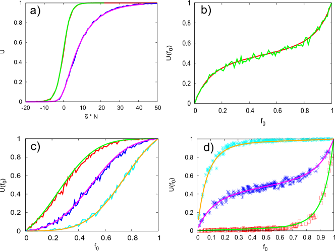
Figure 6: Fixation probabilities $u(\tilde{s},f_{0},N)$in the mutualistic model. Full curves show the analytical results from Eq. (40) with initial fraction $f_{0}=n_{A}(0)/(n_{A}(0)+n_{B}(0)$. a) Competitive exclusion: Simulations with $\epsilon_{A}+\epsilon_{B}=0$ with $-0.08<\epsilon_{A}<0.2,N=250$: Red curve: $f_{0}=0.1$, blue curve $f_{0}=0.5$. Green and purple curves: Eq. (17) with $-0.08<\tilde{s}<0.2,N=250$, $f_{0}=0.1$ (green), $f_{0}=0.5$ (purple). The curves are plotted against the scaling variable $\tilde{s}*N$ for different initial frequencies $f_{0}$. Here (and also in b),c)) the initial condition is chosen on the line $n_{A}(0)+n_{B}(0)=N$. b) Mutualism: Green curve: simulations with $\epsilon_{A}=\epsilon_{B}=0.1,N=100,f^{*}=0.5$. The fixation probability $u$ is plotted versus the initial fraction $f_{0}$. Red curve: Fixation formula (17) with $N=100,\tilde{s}=0.1,f^{*}=0.5$. c) Coordination game with an unstable fixed point $f^{*}$: Green; purple; orange curves: simulations with $\epsilon_{A}=-0.05,\epsilon_{B}=-0.15(f^{*}=0.25);\epsilon_{A}=-0.10,\epsilon_{B}=-0.10(f^{*}=0.50);\epsilon_{A}=-0.15,\epsilon_{B}=-0.05(f^{*}=0.75)$ . Red; blue; cyan curves: Fixation formula (40) with $N=100,\tilde{s}/f^{*}=-0.2,f^{*}=0.25;0.5;0.75$. d) Mutualism with stochastic initial conditions. Simulations with initial conditions $n_{A}(0),n_{B}(0)$ are uniformly distributed in the plane of size $N\times N$ with $N=100$. For each random initial condition, which fixes the value of $f_{0}$, the fixation probability is averaged over 500 independent Gillespie simulations resulting in $u(f_{0})$. Cyan points: $\epsilon_{A}=0.05,\epsilon_{B}=0.15,f^{*}=0.25$; blue points: $\epsilon_{A}=0.10,\epsilon_{B}=0.10,f^{*}=0.5$; red points: $\epsilon_{A}=0.15,\epsilon_{B}=0.05f^{*}=0.75$. Full curves: fixation formula (40) with $N=100,\tilde{s}/f^{*}=0.2$: Brown: $f^{*}=0.25$; purple: $f^{*}=0.25$; green $f^{*}=0.75$.

• $\epsilon_{A}+\epsilon_{B}=0$. Unless $\epsilon_{A}=\epsilon_{B}=0$, this corresponds to a selective advantage under crowded conditions, such that $c_{A}+c_{B}\approx 1$. In the previous section, we discussed how in the deterministic limit there are two stable fixed points, $(c_{A}^{*},c_{B}^{*})=(1,0)$ and $(c_{A}^{*},c_{B}^{*})=(0,1)$, while the fixed point with both $c_{A}^{*}$ and $c_{A}^{*}$ nonzero is inaccessible. Fig. 6a shows the fixation probability for $c_{A}(t=0)+c_{B}(t=0)=1$ and two initial frequencies $f_{0}=0.5$, $f_{0}=0.1$, $N=250$, $f^{*}=\epsilon_{A}/(\epsilon_{A}+\epsilon_{B})$ and effective selective advantage $\tilde{s}=\mu\epsilon_{A}=-\mu\epsilon_{B}$. The population size $N$ appears through the combination $\tilde{s}*N$ in Eq. 40, so we plot the probability versus this rescaled parameter. We obtain excellent agreement between this special case of our model and the Kimura formula for the Moran model Eq. (17).

• $\epsilon_{A}+\epsilon_{B}=\tilde{s}/f^{*},\epsilon_{A}>0,\epsilon_{B}>0$. This corresponds to a mutualistic situation in which there is a stable fixed point out in the plane $(c_{A}^{*}>0,c_{B}^{*}>0)$. Fig. 6b shows the fixation probability $u(f_{0})$ versus the initial fraction $f_{0}$ for stochastic Gillespie simulations with $\epsilon_{A}=\epsilon_{B}=0.1$ where $f^{*}=0.5$ and $N=100$. For comparison, the formula Eq.(40) is shown as the full drawn line again indicating very good agreement.

• $\epsilon_{A}+\epsilon_{B}=-\tilde{s}/f^{*},\epsilon_{A}<0,\epsilon_{B}<0$. This choice corresponds to the competitive exclusion (Frey, 2010) in which there is an unstable fixed point in the plane $(c_{A}^{*}>0,c_{B}^{*}>0)$ and two stable fixed points where one of the two species has gone extinct. Fig. 6c shows Gillespie simulations for three cases of $\epsilon_{A}<0,~{}\epsilon_{B}<0$ and a comparison with the formula Eq. (40) for the different values of $f^{*}$ (in order to compare this case we take $\tilde{s}<0$ in the formula).

As a further case we consider random initial conditions $n_{A}(0),n_{B}(0)$ uniformly distributed in the square $[1,N]\times[1,N]$, so that the approach to the line $c_{A}+c_{B}\approx 1$ can play a role as well. The initial fraction is now defined as $f_{0}=n_{A}(0)/[n_{A}(0)+n_{B}(0)]$. Fig. 6d show the corresponding Gillespie simulation results for 200 different initial conditions for three different fractions $f^{*}=0.25,0.5,0.75$. The analytic fixation curves according to Eq. (40) are also shown. Although the agreement is excellent, we again expect modification when departures from equality of the initial growth rates $\mu_{A}$ and $\mu_{B}$ are allowed.

4 One and two dimensions

Density fluctuations play a more significant role in one and two spatial dimensions, compared with the well-mixed situations described in the previous section. For example, depending on initial conditions and genetic drift, different alleles can fix in different regions of space; the ultimate fate of the system then depends on how these different regions interact, which in turn depends on the choice of the rates. One of the most striking effects of spatial variation in allele number and relative proportions is the existence of a regime in which there is a reduction in the average carrying capacity, i.e. the average concentration $Z$ is smaller than the value $\langle Z\rangle=1$ calculated from Eqs. (2) with our choice of parameters and by neglecting fluctuations. The presence of such a regime is illustrated in Fig. (7) in the neutral case as a function of the $D$ and $N$. Notice that the latter parameter can be properly interpreted as an average number of particles per unit length only when $N$ and $D$ are both large enough. In the opposite regime, as a consequence of fluctuations, the average number of particles in a unit segment is significantly less than $N$. We quantify this effect by defining an effective average carrying capacity $\langle Z\rangle=\langle n(t)\rangle/N$ where $n(t)$ is the actual number of particles present at time $t$ per unit length and the average $\langle\dots\rangle$ is over time.

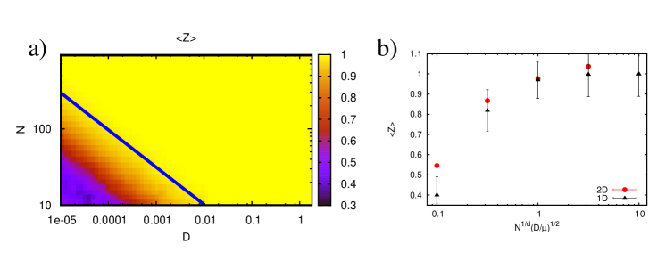
Figure 7: Reduction of the carrying capacity in the neutral model in $1d$ and $2d$. (a) Reduction of the total carrying capacity $Z=\langle c_{A}+c_{B}\rangle$ in the $(D,N)$-plane. The system is one dimensional and we adopted the neutral choice of parameters (see Section 2). The blue line is the theoretical condition $N\sqrt{D}/\mu=1$ . (b) Comparison of the carrying capacity reduction in $1d$ and $2d$, as a function of the nondimensional parameter $N^{1/d}\sqrt{D/\mu}$ where $d$ is the spatial dimension.

We find significant deviations from the prediction $\langle Z\rangle=1$ when $N\sqrt{D/\mu}\ll 1$ . Heuristically, this criterion can be understood as follows. In spatially extended systems, the populations are mixed by diffusion. The diffusion scale $\sqrt{D/\mu}$ may be considered as an “effective deme size”, in the sense that individuals within a distance less than $\sqrt{D/\mu}$ are mixed very efficiently over a single generation, while individuals separated by a larger distance are spatially decoupled. In one dimension, the condition $N\sqrt{D/\mu}\gg 1$ then corresponds to having many individuals in an effective deme size. In the opposite limit, this number is small and fluctuations play a much more important role. This effect is related to the “strong noise limit” of the stochastic Fisher equation (see e.g. Doering et al. (2003); Berti et al. (2007); Hallatschek and Korolev (2009)). We remark that in this regime, the assumptions needed to derive Eq.(2) from the particle model are violated and significant deviations between the particle simulations and the macroscopic theory are expected. For this reason, we will restrict our analysis here to the “weak noise” case in which $N\sqrt{D/\mu}>1$.

4.1 Neutral theory

To study how fixation occurs in space, we now discuss the behavior of the spatial heterozygosity $H(x,t)$ defined as the probability of two individuals at distance $x$ and time $t$ to carry different alleles. In the neutral stepping stone model with a fixed population size in each deme, $H(x,t)$ obeys a closed equation:

$$\partial_{t}H(x,t)=D\nabla^{2}H-\frac{2\mu}{N}H\delta(x).$$ (18)

In one dimension, such equation can be solved explicitly:

$$H(x,t)=H_{0}\left[1-\frac{2}{N}\int_{0}^{t}\ dt^{\prime}\frac{\mathrm{erf}\left(\frac{t^{\prime}}{4N^{2}D}\right)}{\sqrt{8\pi D(t-t^{\prime})}}e^{-\frac{x^{2}}{8D(t-t^{\prime})}+\frac{t^{\prime}}{4N^{2}D}}\right]$$ (19)

where $H_{0}$ is the initial heterozygosity, equal to one half if the two variants are well mixed and equally populated at time $t=0$. Eqs. (18) and (19) can be derived directly from the stochastic Fisher equation (1) with $s=0$ (see, e.g., Korolev et al. (2009)).

We define the heterozygosity in our off-lattice particle simulations with growth and competition from the statistics of interparticle distances. In particular, at a given time $t$, we compute all distances between pairs of individals. Upon introducing a bin size $h$, the function $H(r,t)$ is then defined as the ratio between the number of pairs carrying different alleles at a separation between $r$ and $r+h$, divided by the total number of pairs of all types in the same range of separation. For simplicity, we always took the bin size $h$ equal to the interaction distance $\delta$.

In the limit $N\sqrt{D/\mu}\gg 1$, the spatial heterozygosity obtained by simulations of the neutral off-lattice model shows a remarkable agreement with Eq. (19), as shown in Fig. (8). This correspondence arises because the relative fraction of allele $A$, $f(x,t)=c_{A}/(c_{A}+c_{B})$, obeys a very similar equations as discussed in the mean field case. In Appendix B, we show that the only effect of density fluctuation is an additional effective advection term in the equation for $\partial_{t}f$, equal to $2D(\nabla\log c_{T})\cdot\nabla f$. The appearance of such term was already found in Vlad et al. (2004) in a deterministic version of the model described here. In our case, one can show that since $c_{T}$ obeys a decoupled equation in the neutral case, such term will not affect the equation for the heterozygosity. Indeed, numerical simulation shows that the average spatial heterozygosity in the model reproduces that of the stepping stone model even in the limit of very high diffusivity shown in Fig. 8, panel (b). Panel (c) shows that similar agreements arise comparing numerical integration of Eq. (18) with our off-lattice simulations in two dimensions. At variance with one dimension, where the local heterozygosity $H(0,t)$ decays at long times as $t^{-1/2}$, in two dimension the decay is much slower, $H(0,t)\sim 1/\ln(t)$. Such slow logarithmic decay is confirmed in simulations in panel (d).

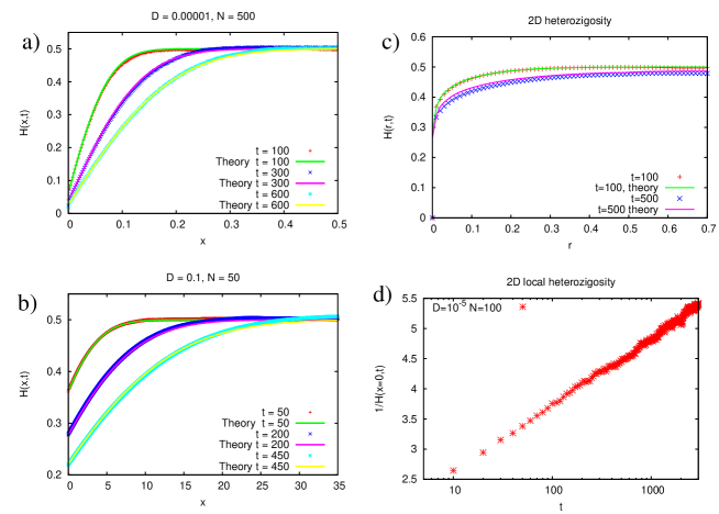
Figure 8: Heterozygosity in the $1d$ and $2d$ neutral case. Behavior of heterozygosity correlation function for the neutral off-lattice model of growth and competition. (a) 1D simulations at low diffusivity, $D=10^{-5}$ and (b) high diffusivity, $D=0.1$. In the top case, the system size is $L=1$ while in the bottom case the system size is $L=100$. In both cases we find excellent agreement with the prediction of formula (19). (c) Neutral heterozygosity in $2d$, compared with a numerical integration of Eq. (18). (d) Behavior of the local heterozygosity $H(x=0,t)$ as a function of time in 2D, showing the logarithmic decay $H(x=0,t)\sim 1/\ln(t)$.

4.2 Reproductive advantage

In one spatial dimension, an analogue of Kimura’s formula (14) (Crow and Kimura, 1970) for the fixation probability has been derived from the stochastic Fisher equation by Doering et al. (2003):

$$p_{fix}=1-\exp\left[-sN\int\ dx\ f(x,t=0)\right]$$ (20)

where $f(x,t=0)$ is the initial spatial distribution of the fraction of species $A$. Remarkably, the one dimensional fixation probability is independent of the spatial diffusion constant. We tested this prediction in Fig. (9a), left panel, for our model when species $A$ enjoys a reproductive advantage $s$. There are again no appreciable differences between the simulations of our more general growth model and the theoretical prediction for the stepping stone model, over a wide range of diffusion constants. This agreement is expected, given the approximate mapping onto a stepping stone model embodied in Eq. (B.3) of Appendix B. While the result (20) by Doering et al. (2003) was derived in one dimension, we conjectured that the same formula holds in two dimensions. Indeed, a straightforward generalization of Eq. (20) predicts well the fixation probability in two dimensions, as shown in simulations in Fig. (9), right panel.

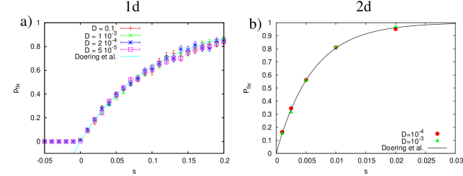
Figure 9: Probabilities of fixation in the presence of a reproductive advantage. The two panels show (a) one spatial dimension and (b) two dimensions, as a function of the selective advantage $s$, for different values of the diffusion constant $D$. Our $1d$ results are compared the results with the prediction of Doering et al. (2003). In 1d, parameters are $N=500$ and the initial fraction of species A is $f_{0}=0.01$, randomly distributed on the unit interval. The $2d$ simulations were conducted on a square domain of unit area and the parameters $N=16384$ and the initial fraction of species A is $f_{0}=0.01$ were kept fixed. The solid line is our conjectured generalization of Eq. (20) to two dimensions.

4.3 Mutualism

We now set $\mu_{A}=\mu_{B}=\mu$, but allow variable interspecific competition coefficients can vary in one and two dimensions. Korolev and Nelson (2011) recently demonstrated how for a mutualistic stepping stone model with fixed deme size in one dimension, there is a region in the $(\epsilon_{A},\epsilon_{B})$ parameter space in which (in limit of an infinite system size, $L\rightarrow\infty$) fixation never occurs, as sketched in Fig. 10, panel a). This behavior differs dramatically from the well-mixed zero dimensional case, for which fixation is inevitable, with a fixation time $t^{*}(\epsilon_{A},\epsilon_{B},N)$ given approximately by Eq. (15).

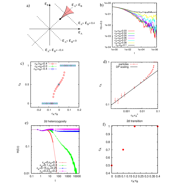
Figure 10: Mutualism in $1d$ and $2d$. a) Phase diagram of the mutualistic model in 1d. The mutualistic region, where global fixation never occurs in an infinite system, is colored in red. Dashed lines denote the cuts relevant to data in the other panels. b) Behavior of the local heterozygosity $H(0,t)$ along the cut $\epsilon_{A}=\epsilon_{B}$. A nonzero long time asymptote implies that fixation never occurs. c) Average concentration of allele $A$, $<c_{A}>$, along three cuts such that $\epsilon_{A}+\epsilon_{B}=const.$. When $\epsilon_{A}+\epsilon_{B}$ is sufficiently large and positive, $\langle f\rangle$ varies smoothly between $0$ and $1$ when traversing the red region in (a). For both $\epsilon_{A}+\epsilon_{B}=0$ and $\epsilon_{A}+\epsilon_{B}$ negative, there is an abrupt jump in $\langle f\rangle$ from $0$ to $1$ when $\epsilon_{A}=\epsilon_{B}$. In this sense, the dashed diagonal line below the cusp in (a) is like a first order phase transition. In all figures, parameters are: $\mu=1$, $D=0.02$, $N=30$ and $L=2000$ so that on average there are $6\cdot 10^{4}$ individuals in the system. d) Logarithmic plot of the density of $A$ close to the critical point. A power law with the expected directed percolation exponent, $f(x)\propto x^{\beta}$, $\beta\approx 0.2765$ is shown for comparison. e) Behavior of the local heterozygosity $H(0,t)$ in $2d$ along the line $\epsilon_{A}=\epsilon_{B}$. A phenomenology similar to the $1d$ case of panel b) is observed. f) Transition along the diagonal cut $\epsilon_{A}+\epsilon_{B}=0.4$ in $2d$, again showing a similar behavior to the $1d$ case shown in panel c).

We fix parameters as $\mu=1$, $D=0.02$ and $N=30$. To explore the behavior of our model, we performed simulations along the paths shown as dashed lines in panel a) of Fig. (10). Panel b) shows the time evolution of the local heterozygosity $H(0,t)$ along the line $\epsilon_{A}=\epsilon_{B}$. For small values of $\epsilon_{A}=\epsilon_{B}>0$, the heterozygosity decays in a similar fashion (roughly as $1/\sqrt{t}$) as in the neutral case $\epsilon_{A}=\epsilon_{B}=0$. For higher values, the local heterozygosity eventually levels off at a nonzero value, implying that fixation will never occur.

The presence of a mutualistic regime where the system remains mixed forever is even more evident in Fig. 10, panel c), where we plot along the cuts at constant $\epsilon_{A}+\epsilon_{B}$ the long-time average of the fraction of the first allele $\langle f\rangle$ as a function of the difference $\epsilon_{A}-\epsilon_{B}$. Along the cuts that do not cross the mutualistic region, $\langle f\rangle$ is either $0$ or $1$ as one of the two alleles always fixes. A special case arises for $\epsilon_{A}=\epsilon_{B}$, where each of the two alleles has a chance of being fixated equal to its relative abundance in the initial condition, so that $\langle f\rangle=f_{0}$. Conversely, $\langle f\rangle$ has a non-trivial behavior along the line $\epsilon_{A}+\epsilon_{B}=0.4$. Upon varying the parameter $\rho=\epsilon_{A}-\epsilon_{B}$, we find a whole range of values in which fixation does not occur. As discussed in (Korolev and Nelson, 2011), the two lines of critical points shown in (a) are in the directed percolation universality class. The behavior of the density close to this critical point is described by a universal exponent, $c_{A}\sim(\epsilon_{A}-\epsilon_{c})^{\beta}$, where the expected exponent is $\beta\approx 0.2765$ and $\epsilon_{c}$ is the value of $\epsilon_{A}$ at the critical point (see e.g. Odor (2004)). Fig. 10, panel d) confirms the power law behavior close to one of the critical points on the cut $\epsilon_{A}+\epsilon_{B}=0.4$. Finally, in panels e) and f) we show simulations on the two dimensional mutualistic model. Mutualism in $2d$ is computationally challenging and, to the best of our knowledge, has not been studied systematically in the literature. Although we did not obtain the full phase diagram, our simulations suggest a scenario similar to the $1d$ case. In particular, the heterozygosity $H(x=0,t)$ along the cut $\epsilon_{A}=\epsilon_{B}$ displays a transition from a regime in which it seems to decay logarithmically (as in the $2d$ neutral version of the model) to a regime in which fixation does not occur. Furthermore, the cut at $\epsilon_{A}+\epsilon_{B}=0.4$ shown in panel f) reveals a directed-percolation-like transition, qualitatively similar to that in panel c).

5 Population genetics in two-dimensional compressible turbulence

A systematic exploration of the effect of hydrodynamic flows on the off-lattice models of population genetics introduced here would take us far beyond the scope of this already lengthy paper. However, to illustrate the interesting effects that arise, we now extend our analysis to the two cases where the competition between populations takes place under the influence of compressible fluid advection in two-dimensions. As we will show, compressible fluid flows can dramatically change the carrying capacities and fixation times. For all the simulations in this section we choose a square simulation domain of size $[0,L]\times[0,L]$, the spatial diffusivity $D=10^{-4}$. For simplicity, the two competing populations are neutral with $\mu_{A}=\mu_{B}=\lambda_{AA}=\lambda_{AB}=\lambda_{BA}=\lambda_{BB}=1$.

The two flows that we choose are:

1. Compressible surface flow (CSF):
   This chaotic, time-dependent flow is generated from a two-dimensional slice of a three-dimensional, homogeneous, isotropic flow (see Perlekar et al. (2010, 2012)). A snapshot of the advecting velocity field is shown on the left side of Fig. 11. Using the projection method described in Perlekar et al. (2012) we choose the compressibility of the flow $\kappa=1$ where, $\kappa\equiv\langle(\nabla\cdot{\bf u})^{2}\rangle/\langle(\nabla{\bf u})^{2}\rangle$, ${\bf u}\equiv(u_{x},u_{y})$ is the velocity field, and $\langle(\cdot)\rangle$ indicate the spatio-temporal averaging. Setting $\kappa$ to its maximum value of unity maximizes the reduction in carrying capacity caused by locally compressing the populations to high density, so that the middle terms on the right side of Eqn. (3) are negative [Pigolotti et al. (2012); Perlekar et al. (2012)]. The strength of the flow is varied by scaling the velocity field by a forcing amplitude $F$. For all the simulations with this flow we choose $L=2\pi$.

2. Steady flow (SF):
   This time-independent velocity field is chosen to be $u_{x}(x,y)=F[\alpha\sin(2\pi x/L)+(1-\alpha)\sin(2\pi y/L)]$, $u_{y}(x,y)=F[\alpha\sin(2\pi y/L)-(1-\alpha)\sin(2\pi x/L)]$ (see Fig. 11 right panel). The strength of the flow is controlled by again changing $F$ and the compressibility $\kappa=\alpha^{2}/[\alpha^{2}+(1-\alpha^{2})]$ is modified by changing $\alpha$ and hence $\kappa\in[0,1]$. For all the simulations with this flow we choose $L=1$. The two species are advected by the flow towards the sink which is located at the center $(-L/2,L/2)$ of the simulation domain.

   

   

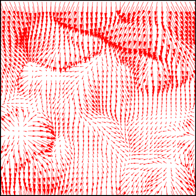
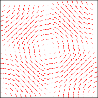
   Figure 11: (Left) A representative snapshot of the time-dependent compressible surface flow (CSF) field used for advecting species in our two-dimensional simulations. (Right) Vector field visualization of the steady flow (SF) used for advecting species in our simulations of a simple time-independent steady flow with $\kappa=0.0027$.

Similar analysis for one-dimensional flows was conducted in Pigolotti et al. (2012). The compressible flow on the left of Fig. 11 models photosynthetic organisms that control their buoyancy to remain near the surface of a turbulent ocean. The flow on the right is designed to determine the consequences for population genetics of fluid sink at the center, with fluid injection at the four corners. Note the non-zero vorticity in this case.

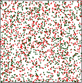
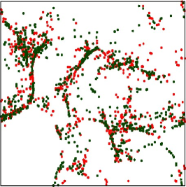
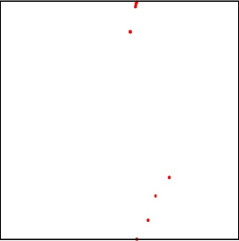
Figure 12: Competition between two neutral species (shown in red and green) in a turbulent compressible flow with $\kappa=1$ and $F=1$. At time $t=0$ (left) approximately $10000$ organisms are randomly distributed over the entire domain at the steady state carrying capacity in absence of flow. Both species are then collapsed by advection onto filamentous structures leading to (time-dependent) sinks and saddle points, dynamics which compactifies the population into regions where competition takes place. This collapse is highlighted in the middle plot which is chosen at a later time $t=1$ (middle). At much later times $t=25$ (right) fixation occurs and only one of the species survive. The populations size has stabilized at $6$ organisms, a reduction from the initial carrying capacity by a factor $10^{3}$. Although the reduction in the population size is most extreme for $\kappa=1$, significant reductions occur for even small values of $\kappa$ [Perlekar et al. (2012)].

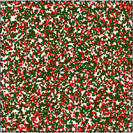
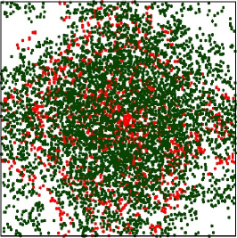
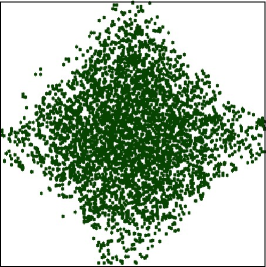
Figure 13: Competition between two neutral species (shown in red and green) in the steady flow with $\kappa=0.0027$. At time $t=0$ (left), the species are randomly distributed over the entire domain again at the equilibrium carrying capacity possible in absence of flow. Species are rotated and collapsed by the advecting flow towards the origin where competition takes place. This progression is highlighted in the middle plot which is chosen at a later time $t=17$ (middle). At much later times $t=41$ (right) fixation occurs and only one of the species survive.

The competition between species for the two flow conditions described above is shown in Figs. 12 and 13. Initially the populations are well-mixed at the steady state carrying capacity as they would be with ordinary diffusion, birth, and competitive death in absence of advection. Advection moves the population towards the localized sinks of the flow and enhances the competitive death embodied in the $\lambda_{ij}$ couplings. Indeed, the middle frames of Figs. 12 and 13 show explicitly the compression that leads to enhanced inter-species and intra-species competition. Eventually at later times, only one species survives [right hand frames of Figs. 12 and 13]. Although the extreme ($10^{3}$-fold!) reduction in population size shown in Fig. 13 results from the use of a maximally compressible ($\kappa=1$) turbulent flow, reductions of $80\%$ arise for $k=0.17$ [Perlekar et al. (2010)] and even for much smaller value of $\kappa$ [Perlekar et al. (2012)].

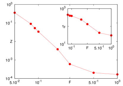
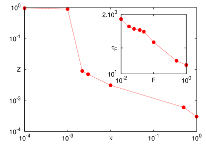
Figure 14: (Left) Carrying capacity for the turbulent compressible flow for varying forcing strength with $\kappa=1$. $Z$ drops with increasing forcing strength. (Right) Carrying capacity for the steady flow at varying compressibility levels. For very small compressibility, carrying capacity is close to the one in absence of flow and then drops. For the extreme case of $\kappa=1$, carrying capacity is reduced by a factor of $10^{3}$, similar to the reduction found when $\kappa=1$ for the compressible surface flow. In both cases, the inset reveals the drop in the fixation times for varying forcing at $\kappa=1$.

To quantify how advecting compressible flows affect carrying capacity and the fixation times, we systematically vary the strength of the flow $F$. Fig. 14(left) shows that on increasing $F$, the carrying capacity drops, due to enhanced confinement and hence competition between the species. On the other hand, using the steady flow we show that at fixed forcing strength, carrying capacity is also reduced on increasing the compressibility [see Fig. 14(right)]. The insets to these figures show the corresponding reduction in the fixation times.

6 Conclusions

The understanding of growth, competition, cooperation and diffusion in space in individual based models has been subject of intense study, in contexts as diverse as population genetics (Barton et al., 2002), ecology (Law et al., 2003; Birch and Young, 2006) and physics (Hernandez-Garcia and Lopez, 2004; Berti et al., 2007; Korolev et al., 2009). A main focus has been to explore the regime in which discreteness effects are such that individual based simulations differ significatively from the behavior of macroscopic continuum equations, such as the Fisher equation or its stochastic variant.

In this paper, we have explored competition and cooperation between two different alleles when the total population size is not constrained. We have deliberately focused on the weak noise limit by choosing carrying capacities and diffusion constants such that there is a good agreement between the outcome of the macroscopic Langevin equations and the individual based simulations.

We have shown that, in certain limits, one can draw an explicit correspondence with stepping stone-like models in which the total density of individuals is kept fixed at every deme, by studying the relative fraction of one of the two species. In the neutral case, the fluctuating total density appear in the equation for the relative fraction, but its fluctuations average out in the equation for mean quantities such as the heterozygosity. The correspondence between stepping stone models and our generalized off-lattice model with additional fluctuations in the overall density was confirmed by individual based simulations. In non-neutral settings, the total density does not obey a closed equation and such exact correspondence can not be drawn. However, we have shown how, when the departure from neutrality is not severe (small $s$ or small $\epsilon_{A}$ and $\epsilon_{B}$), the corrections due to density fluctuations can be safely neglected and the predictions of constant-density models are still reproduced with accuracy. The issue we address here is a more subtle dynamical version of justifying the neglect of number fluctuations in the grand canonical ensemble as compared to the canonical ensemble in equilibrium statistical mechanics. We conclude that the model we present here is a natural candidate to study situations in which the total density of individuals can vary greatly from the background carrying capacity due to external forces, such as turbulence or compressible fluid flows (Pigolotti et al., 2012).

Acknowledgements: Some of the computations in this paper were run on the Odyssey cluster supported by the FAS Science Division Research Computing Group at Harvard University. Work by DRN was supported through the National Science Foundation, via Grant DMR1005289 and through the Harvard Materials Research Science and Engineering Center, through grant DMR0820484. We thank K. Korolev for comments on the manuscript.

Appendix A Derivation of the macroscopic equations

In this section we present an explicit derivation of the coupled stochastic macroscopic equations for $c_{A}(x,t)$ and $c_{B}(x,t)$, Eq.(2), from the microscopic rate reactions (2). The formalism we will follow is that of the chemical master equation, as presented for example by Gardiner (2004), which in turn may be considered as a spatial generalization of the Kramers-Moyal expansion (Gardiner, 2004; Risken, 1989).

As discussed in the section 2, we consider interacting individuals in a volume equal to $L^{d}$ in $d$ dimensions. In particular, competition occurs when individuals are within a small volume $\delta$ (for details on the implementation of the individual-based dynamics see Perlekar et al. (2011)). We can then discretize the system in cells of size $\delta$ and start the derivation from the master equation governing the time evolution of the probability of the numbers of particles $\{n_{j}^{A},n_{j}^{B}\}$ of type $A$ and $B$ in each cell, labeled by the index $j$. We first define as $W_{A}(\pm 1,n_{j}^{A},n_{j}^{B})$ and $W_{B}(\pm 1,n_{j}^{A},n_{j}^{B})$ the rates at which the populations of type $A$ (or $B$) increase/decrease by one individual in a specific box, given that the numbers are currently $n^{A}_{j}$ and $n^{B}_{j}$. The expression for these rates are then:

$$W_{A}(+1,n_{j}^{A},n_{j}^{B}) = \mu_{A}n_{j}^{A}$$

$$W_{A}(-1,n_{j}^{A},n_{j}^{B}) = \tilde{\lambda}_{AA}n_{j}^{A}(n_{j}^{A}-1)+\tilde{\lambda}_{AB}n_{j}^{A}n_{j}^{B}$$

$$W_{B}(+1,n_{j}^{A},n_{j}^{B}) = \mu_{A}n_{j}^{B}$$

$$W_{B}(-1,n_{j}^{A},n_{j}^{B}) = \tilde{\lambda}_{BA}n_{j}^{A}n_{j}^{B}+\tilde{\lambda}_{BB}n_{j}^{B}(n_{j}^{B}-1).$$ (21)

The master equation governing the evolution of the full probability distribution $P(\{n_{j}^{A},n_{j}^{B}\},t)$ for all possible box occupation numbers $\{n^{A}_{j},n^{B}_{j}\}$ then reads:

$$\frac{d}{dt}P(\{n_{j}^{A},n_{j}^{B}\},t) = \sum_{j}\left[W_{A}(+1,n_{j}^{A}-1,n_{j}^{B})P(n_{1}^{A},\dots,n_{j}^{A}-1,\dots,n_{1}^{B},\dots)-W_{A}(+1,n_{j}^{A},n_{j}^{B})P(\{n_{j}^{A},n_{j}^{B}\})\right]$$ (22)

$$+ \sum_{j}\left[W_{A}(-1,n_{j}^{A}+1,n_{j}^{B})P(n_{1}^{A},\dots,n_{j}^{A}+1,\dots,n_{1}^{B},\dots)-W_{A}(-1,n_{j}^{A},n_{j}^{B})P(\{n_{j}^{A},n_{j}^{B}\})\right]$$

$$+ \sum_{j}\left[W_{B}(+1,n_{j}^{A},n_{j}^{B}-1)P(n_{1}^{A},\dots,n_{1}^{B},\dots,n_{j}^{B}-1,\dots)-W_{B}(+1,n_{j}^{A},n_{j}^{B})P(\{n_{j}^{A},n_{j}^{B}\})\right]$$

$$+ \sum_{j}\left[W_{B}(-1,n_{j}^{A},n_{j}^{B}+1)P(n_{1}^{A},\dots,n_{1}^{B},\dots,n_{j}^{B}+1,\dots)-W_{B}(-1,n_{j}^{A},n_{j}^{B})P(\{n_{j}^{A},n_{j}^{B}\})\right]$$

$$+ \mathrm{diffusion}\ \mathrm{terms},$$

where the diffusion terms allow for the stochastic exchange of particles between neighboring boxes. Although we did not write them explicitly, they reduce to discrete approximations to Laplace operator. Indeed, we replace them with Laplacians in the continuous space limit at the end of the calculation.

The next step in the derivation is to perform a Kramers-Moyal expansion (Risken, 1989) in each of the boxes, which leads to

$$\partial_{t}P(\{n_{j}^{A},n_{j}^{B}\})=\sum\limits_{j}\sum\limits_{k=1}^{\infty}\frac{(-1)^{k}}{k!}\{\partial^{k}_{n_{j}^{A}}[\alpha^{A}_{k}(n_{j}^{A},n_{j}^{B})P(\{n_{j}^{A},n_{j}^{B}\})]+\partial^{k}_{n_{j}^{B}}[\alpha^{B}_{k}(n_{j}^{A},n_{j}^{B})P(\{n_{j}^{A},n_{j}^{B}\})]\},$$ (23)

with

$$\alpha_{k}^{A,B}(n_{j}^{A},n_{j}^{B})=\int d\Delta n_{j}^{A,B}\ (\Delta n_{j}^{A,B})^{k}W_{A,B}(\Delta n_{j}^{A,B},n_{j}^{A},n_{j}^{B}),$$ (24)

and where the integral over $\Delta n$ accounts for the possible jump processes ($+1$ and $-1$ in our case). Finally, truncating the Kramers-Moyal expansion up to second order in the derivatives leads to a Fokker-Planck equation for $P\{n_{j}^{A},n_{j}^{B}\}$. It is convenient to write directly the equivalent but somewhat simpler system of Langevin equations corresponding to this Fokker-Planck description, namely:

$$\frac{dn_{j}^{A}}{dt}=n_{j}^{A}(\mu_{A}-\tilde{\lambda}_{AA}n_{j}^{A}-\tilde{\lambda}_{AB}n_{j}^{B})+\mathrm{diffusion}+\sqrt{n_{j}^{A}(\mu_{A}+\tilde{\lambda}_{AA}n_{j}^{A}+\tilde{\lambda}_{AB}n_{j}^{B})}\xi_{j}^{A}$$

$$\frac{dn_{j}^{B}}{dt}=n_{j}^{B}(\mu_{B}-\tilde{\lambda}_{BA}n_{j}^{A}-\tilde{\lambda}_{BB}n_{j}^{B})+\mathrm{diffusion}+\sqrt{n_{j}^{B}(\mu_{B}+\tilde{\lambda}_{BA}n_{j}^{A}+\tilde{\lambda}_{BB}n_{j}^{B})}\xi_{j}^{B}.$$ (25)

In the above system of equations, the $\xi$’s are delta-correlated unit variance Gaussian processes, $<\xi_{j}^{k}(t)\xi_{l}^{m}(t^{\prime})>=\delta_{jl}\delta_{km}\delta(t-t^{\prime})$. The multiplicative noise in the equation must be interpreted according to the Ito prescription (Gardiner, 2004; Korolev et al., 2009). In principle, the diffusion terms in (22) would contribute to the noise term. However, one can show that this contribution can be neglected if the size of the cells is sufficiently large (see Gardiner (2004)).

From Eqs.(A) one can finally derive Eqs. (2) by:

1. Taking (formally) the limit $\delta\rightarrow 0$. In such a way the number densities of individuals are continuous functions of the coordinate $\mathbf{x}$, $n_{A}(\mathbf{x},t)$ and $n_{B}(\mathbf{x},t)$.

2. Defining rescaled, macroscopic rates of binary reactions,

   $$\lambda_{ij}=N\delta\tilde{\lambda}_{ij}$$ (26)

3. Defining the macroscopic concentrations of individuals $c_{A,B}(\mathbf{x},t)=n_{A,B}(\mathbf{x},t)/N$.

The convenience of introducing the macroscopic binary reaction rates $\lambda_{ij}$ in step (2) is that the microscopic interaction radius $\delta$ does not appear in the macroscopic system of equations (2). At the same time, we introduced a parameter $N=\lambda_{ij}/(\delta\tilde{\lambda}_{ij})$ that, as clear from step (3) in the above procedure, sets the typical number density of particles corresponding to a macroscopic concentration $c(\mathbf{x},t)=1$. Such parameter does not appear in the deterministic drift terms of the equation but only in the noise terms, whose amplitude vanishes for $N\rightarrow\infty$. It is worthwhile remarking that, while we followed here the Kramers-Moyal expansion procedure, in the Van Kampen formalism the parameter $N^{-1}$ is the relevant expansion parameter which is assumed to be small (Risken, 1989; Gardiner, 2004).

We remark that through the paper we presented only results of the particle models, corresponding to given parameter choices in the macroscopic equations (2). Equation (26) can be seen as defining the mapping between the parameters used in the particle simulations (the interaction domain $\delta$ and the microscopic binary rates $\tilde{\lambda}_{ij}$’s) and those appearing in the macroscopic description ($N$ and the set of $\lambda_{ij}$’s) The same relation can be used for the reverse task, i.e. finding microscopic parameters $\delta$ and $\tilde{\lambda}_{ij}$’s corresponding to given $N$ and $\lambda_{ij}$’s. Clearly this mapping is not univoquely determined, but has one degree of freedom. As sketched in Sec. (2), we fixed this degree of freedom in two different ways in the well-mixed version of the model and in the $d>0$, spatially explicit simulations. In particular, in $d=0$ we chose $\delta=1$, so that the microscopic binary reaction rates are $N$ times smaller than the macroscopic ones, $\tilde{\lambda}_{ij}=\lambda_{ij}/N$. In this case, it is crucial to set the system size $L=1$ so that all particles interact with all other particles. Instead, in $d>0$ we chose the interaction domain $\delta=1/N$, so that the microscopic and macroscopic reaction rates are identical, $\tilde{\lambda}_{ij}=\lambda_{ij}$. Further details on the simulation schemes can be found in Perlekar et al. (2011).

We conclude this Appendix by noting that the continuous space limit is a formal one, and cannot be performed in a rigorous way. One of several subtleties is that neglect of the diffusive contribution to the noise variance requires a finite value of $\delta$, so that the limit of vanishingly small interaction range cannot be taken in a strict sense. Thus, Eq. (22) should be regarded as a continuum shorthand notation: In practice, we always simulate equations such as Eq. (A) on a lattice of finite size, and require a smoothly varying total density of particles. When this assumption is invalid, the macroscopic description can break down, as briefly discussed in the beginning of section (4) for the problem of the reduction in the total number of particles for $d=1$ and $d=2$.

Appendix B Appendix: equations for the relative fraction of one species

The correspondence between the growth model presented here and the stepping stone model with Fisher-Wright or Moran dynamics, or the equivalent stochastic Fisher-Kolmogorov-Petrovsky-Piscounov equation (Fisher, 1937; Kolmogorov et al., 1937) can be illuminated by constructing the dynamical equation for the relative fraction of species $A$, $f=c_{A}/c_{T}$ with $c_{T}=c_{A}+c_{B}$. A dynamical equation for $f$ can be derived with help of the Ito calculus: upon writing the system of equation (2) as:

$$\frac{d}{dt}c_{A}(\mathbf{x},t) = \alpha_{A}(c_{A},c_{B})+\sigma_{A}(c_{A},c_{B})\xi(\mathbf{x},t)$$

$$\frac{d}{dt}c_{B}(\mathbf{x},t) = \alpha_{B}(c_{A},c_{B})+\sigma_{B}(c_{A},c_{B})\xi^{\prime}(\mathbf{x},t)$$ (27)

where the diffusive Laplacian terms are included into $\alpha_{A}$, $\alpha_{B}$. The equation for the $A$-fraction $f$ then reads

$$\frac{d}{dt}f = \alpha_{A}\partial_{A}f+\alpha_{B}\partial_{B}f+\sqrt{\sigma_{A}^{2}(\partial_{A}f)^{2}+\sigma_{B}^{2}(\partial_{B}f)^{2}}\xi+$$ (28)

$$+ \frac{\sigma^{2}_{A}}{2}\partial_{AA}f+\frac{\sigma^{2}_{B}}{2}\partial_{BB}f,$$

where we used the abbreviated notation $\partial_{A}\equiv\partial_{c_{A}}$, $\partial_{AA}\equiv\partial^{2}_{c_{A}}$ and so on. Inserting the complete set of equations 2 into (28) leads to a lengthy expression for the dynamics of$f$. However, with the choice of parameters we made to discuss a reproductive advantage (this reduces to the neutral case for $s=0$), Eq.(28) simplifies to

$$\frac{\partial}{\partial t}f = D\nabla^{2}f+2D\nabla(\log c_{T})\cdot\nabla f+$$ (29)

$$+ \mu sf(1-f)+\frac{\mu sf}{c_{T}N}(f-1)+\sqrt{\mu f(1-f)\frac{1+c_{T}}{Nc_{T}}+\frac{\mu sf}{Nc_{T}}(1-f)^{2}}\xi.$$

Upon neglecting small contributions of order $s/N\ll 1$ in the last two terms and neglecting fluctuations in the total density (i.e. imposing $c_{T}=1$), we recover exactly the equation (1) governing the macroscopic dynamics of the stepping stone model.

Repeating the calculation in the case of mutualism yields:

$$\frac{\partial}{\partial t}f = D\nabla^{2}f+2D\nabla(\log c_{T})\cdot\nabla f+\mu f(1-f)[\epsilon_{A}-(\epsilon_{A}+\epsilon_{B})f]+$$ (30)

$$+ \frac{\mu f(f-1)}{N}[\epsilon_{A}(f-1)+\epsilon_{B}f]+\sqrt{\frac{\mu f(1-f)\left[\left(\frac{1+c_{T}}{c_{T}}\right)-\epsilon_{A}(1-f)^{2}-\epsilon_{B}f^{2}\right]}{N}}\xi$$

Upon neglecting, similar to the case of reproductive advantage, terms order $\epsilon_{A,B}/N$, and again neglecting fluctuations away from the line $c_{T}(\mathbf{x},t)=c_{A}(\mathbf{x},t)+c_{B}(\mathbf{x},t)=1$, we recover the continuum limit of the mutualistic stepping stone model treated by Korolev and Nelson (2011), namely

$$\frac{\partial}{\partial t}f=D\nabla^{2}f+s_{0}f(1-f)(f^{*}-f)+\sqrt{\frac{2\mu f(1-f)}{N}}\xi(\mathbf{x},t),$$ (31)

where $s_{0}=\mu(\epsilon_{A}+\epsilon_{B})$ and $f^{*}=\epsilon_{A}/(\epsilon_{A}+\epsilon_{B})$.

Appendix C Appendix: Fixation times for the mutualistic model in the well-mixed case

To estimate the average fixation time for the mutualistic model in the well-mixed limit, we start from Eq. 30. Upon neglecting terms order $\epsilon_{A}/N$, $\epsilon_{B}/N$ and also neglecting density fluctuations by imposing $c_{T}=c_{A}+c_{B}=1$, we obtain:

$$\frac{d}{dt}f\approx\mu f(1-f)[\epsilon_{A}-(\epsilon_{A}+\epsilon_{B})f]+\sqrt{\frac{2\mu f(1-f)}{N}}\xi.$$ (32)

The dynamics of such equation will reach one of the two absorbing states at $f=0$ or $f=1$ for long enough times. However, these times can be very long when $N$ is large: a time-independent metastable probability distribution exists before the absorbing states are reached, which can be written using potential methods (Gardiner, 2004) as

$$\mathcal{P}(f)\propto e^{-V(f)}$$ (33)

where the potential $V$ is given by

$$V(f)=-Nf\left[\epsilon_{A}-\frac{(\epsilon_{A}+\epsilon_{B})}{2}f\right]+\ln[f(1-f)]$$ (34)

where the first term is analogous to a potential energy and the second resembles an entropy. In the large $N$ limit, the potential has a minimum at $f^{c}\approx\epsilon_{A}/(\epsilon_{A}+\epsilon_{B})$ and two maxima, one at $f^{-}\approx 1/(N\epsilon_{A})$ and one at $f^{+}\approx 1-1/(N\epsilon_{B})$. By evaluating the potential at these points one can estimate the lifetime of the metastable state from the height of the two potential barriers. To the leading order in $N$, the smallest barrier is given by:

$$\Delta V=\frac{N}{2}\frac{\min(\epsilon_{A}^{2},\epsilon_{B}^{2})}{\epsilon_{A}+\epsilon_{B}}.$$ (35)

Finally, we assume that fixation always occurs via the smallest barrier. With this assumption, the time needed to escape the potential minimum to one of the absorbing state can be simply estimated from Kramer’s escape rate theory as $t^{*}\sim\exp(\Delta V)$, which leads to Eq.(15).

We now discuss the fixation probability in zero dimensions. The Kolmogorov backward equation corresponding to the stochastic differential equation (32), when interpreted using the Ito calculus, reads:

$$\frac{\partial u(p,t)}{\partial t}=\frac{1}{N}p(1-p)\frac{\partial^{2}}{\partial p^{2}}u(p,t)~{}+\tilde{s}p(1-p)(f^{*}-p)\frac{\partial}{\partial p}u(p,t),$$ (36)

where $u(p,t)$ is the probability that species A has fixed at time $t>0$ given that it was present with frequency $p$ at time $t=0$. We have set $f^{*}=\epsilon_{A}/(\epsilon_{A}+\epsilon_{B})$, and defined the mutualistic advantage $\tilde{s}=\mu(\epsilon_{A}+\epsilon_{B})$.

Note that Eq. 36 includes the original Kimura problem of two non-interacting species as a special case, in the limit $f^{*}\to\infty,\tilde{s}\to 0$ with the selective advantage given by the fixed product, $s\equiv f^{*}\tilde{s}\equiv\mu\epsilon_{A}$. We now define the long time fixation probability for the initial condition $p=f_{0}$ as

$$\lim_{t\to\infty}u(f_{0},t)\equiv u(f_{0})$$ (37)

Upon assuming a steady state arises at long times, we have from Eq. (36)

$$\frac{d}{dp}u^{\prime}(p)~{}=~{}Ns(f^{*}-p)u^{\prime}(p)$$ (38)

which leads to

$$u^{\prime}(p)~{}=~{}C~{}e^{\frac{1}{2}Ns(f^{*}-p)^{2}}$$ (39)

With boundary conditions $u(0)=0,~{}u(1)=1$, we integrate once more to obtain the fixation probability (Korolev and Nelson, 2011)

$$u(f_{0})~{}=~{}\frac{\int_{0}^{f_{0}}e^{\frac{1}{2}Ns(f^{*}-p)^{2}}dp}{\int_{0}^{1}e^{\frac{1}{2}Ns(f^{*}-p)^{2}}dp}~{}~{},$$ (40)

a closed form expression in terms of the parameters $f_{0},f^{*},N~{}{\rm and}~{}s$. It is straightforward to show that in the limit $f^{*}\to 0,s\to 0$ with $\tilde{s}\equiv f^{*}s$ fixed (two noninteracting species with a selective advantage $\tilde{s}$) we recover Kimura’s famous formula for the fixation probability, Eq. (17).

References

- Barton et al. (2002) Barton, N. H., Depaulis, F., Etheridge, A. M., 2002. Neutral evolution in spatially continuous populations. Theoretical Population Biology 61, 31–48.
- Benzi et al. (2012) Benzi, R., Jensen, M. H., Nelson, D. R., Perlekar, P., Pigolotti, S., Toschi, F., 2012. Population dynamics in compressible flows. European Physical Journal: Special Topics 204 (1), 57–73.
- Berti et al. (2007) Berti, S., Lopez, C., Vergni, D., Vulpiani, A., 2007. Discreteness effects in a reacting system of particles with finite interaction radius. Phys. Rev. E 76, 031139.
- Birch and Young (2006) Birch, D. A., Young, W. A., 2006. A master equation for a spatial population model with pair interactions. Theo. Pop. Biol. 70 (1), 26–42.
- Cencini et al. (2012) Cencini, M., Pigolotti, S., noz, M. A. M., 2012. What ecological factors shape species-area curves in neutral models? Plos One 7 (6), e38232.
- Crow and Kimura (1970) Crow, J., Kimura, M., 1970. Introduction to Population Genetics Theory. Harper & Row Publishers.
- Doering et al. (2003) Doering, C., Mueller, C., Smereka, P., 2003. Interacting particles, the stochastic fisher-kolmogorov–petrovsky–piscounov equation, and duality. Physica A 325, 243–259.
- D’Ovidio et al. (2010) D’Ovidio, F., Monte, S. D., Alvain, S., Dandonneau, Y., Levy, M., 2010. Fluid dynamical niches of phytoplankton types. Proc. Natl. Acad. Sci. 107, 18366–18370.
- Fisher (1937) Fisher, R., 1937. The wave of advance of advantageous genes. Ann. Eugenics 7, 353.
- Frey (2010) Frey, E., 2010. Evolutionary game theory: Theoretical concepts and applications to microbial communities. Physica A 389, 4265.
- Gardiner (2004) Gardiner, C., 2004. Handbook of Stochastic Methods. Springer.
- Hallatschek and Korolev (2009) Hallatschek, O., Korolev, K., 2009. Fisher waves in the strong noise limit. Physical Review Letters 103, 108103.
- Hernandez-Garcia and Lopez (2004) Hernandez-Garcia, E., Lopez, C., 2004. Clustering, advection and patterns in a model of population dynamics with neighborhood-dependent rates. Phys. Rev. E 70 (1), 016216.
- Kimura (1953) Kimura, M., 1953. ”stepping stone” model of population. Ann. Rept. Nat. Inst. Genetics 3, 62–63.
- Kimura and Weiss (1964) Kimura, M., Weiss, G. H., 1964. The stepping stone model of population structure and the decrease of genetic correlation with distance. Genetics 49, 561–576.
- Kolmogorov et al. (1937) Kolmogorov, A., Petrovsky, N., Piscounov, N., 1937. Study of the diffusion equation with growth of the quantity of matter and its application to a biology problem. Moscow Univ. Math. Bull. 1, 1.
- Korolev et al. (2009) Korolev, K., Avlund, M., Hallatschek, O., Nelson, D., 2009. Genetic demixing and evolutionary forces in the one-dimensional stepping stone model. Review of Modern Physics 82, 1691–1718.
- Korolev et al. (2012) Korolev, K., Muller, M., Murray, A. W., Hallatscheck, O., Nelson, D. R., 2012. Selective sweeps in growing microbial colonies. Physical Biology 9, 026008.
- Korolev and Nelson (2011) Korolev, K., Nelson, D., 2011. Competition and cooperation in one-dimensional stepping-stone models. Physical Review Letters 107, 088103.
- Law et al. (2003) Law, R., Murrell, D. J., Dieckmann, U., 2003. Population growth in space and time: the spatial logistic equation. Ecology 84 (1), 252–262.
- Neufeld and Hernandez-Garcia (2009) Neufeld, Z., Hernandez-Garcia, E., 2009. Chemical and Biological Processes in Fluid Flows. A dynamical systems approach. Imperial College Press.
- Neuhauser (1991) Neuhauser, C., 1991. Ergodic theorems for the multitype contact process. Probab. Theory Relat. Fields 91, 467–506.
- Odor (2004) Odor, G., 2004. Universality classes in nonequilibrium lattice systems. Rev. Mod. Phys 76, 663–724.
- O’Malley et al. (2006a) O’Malley, L., Basham, J., Yasi, J. A., Korniss, G., Allstadt, A., Caraco, T., 2006a. Invasive advance of an advantageous mutation: Nucleation theory. Theo. Pop. Biol. 70, 467–478.
- O’Malley et al. (2006b) O’Malley, L., Kozma, B., Korniss, G., Racz, Z., Caraco, T., 2006b. Fisher waves and front roughening in a two-species invasion model with preemptive competition. Phys. Rev. E 74, 041116.
- Perlekar et al. (2010) Perlekar, P., Benzi, R., Nelson, D., Toschi, F., 2010. Population dynamics at high reynolds number. Physical Review Letters 105, 144501.
- Perlekar et al. (2012) Perlekar, P., Benzi, R., Nelson, D. R., Toschi, F., 2012. Population dynamics in compressible flows. arxiv/1203.6319.
- Perlekar et al. (2011) Perlekar, P., Benzi, R., Pigolotti, S., Toschi, F., 2011. Particle algorithms for population dynamics in flows. Journal of Physics: Conference Series 333, 012013.
- Pigolotti et al. (2012) Pigolotti, S., Benzi, R., Jensen, M., Nelson, D., 2012. Population genetics in compressible flows. Physical Review Letters 108, 128102.
- Pringle et al. (2011) Pringle, J. M., Blakeslee, A. M. H., Byers, J. E., Roman, J., 2011. Asymmetric dispersal allows an upstream region to control population structure throughout a species’ range. Proc. Natl. Acad. Sci. 108, 15288–15293.
- Risken (1989) Risken, H., 1989. The Fokker-Planck equation: Methods of Solution and Applications. Springer, Berlin.
- Smith (1998) Smith, J. M., 1998. Evolutionary Genetics. Oxford University Press.
- spatial competition under a reproduction–mortality constraint (2009) spatial competition under a reproduction–mortality constraint, P., 2009. A. allstadt and t. caraco and g. korniss. Jour. Theo. Biol. 258, 537–549.
- Tel et al. (2005) Tel, T., de Moura, A., Grebogi, C., Karolyi, G., 2005. Chemical and biological activity in open flows: A dynamical system approach. Physics Report 413 (2-3), 91–196.
- Vlad et al. (2004) Vlad, M., Cavalli-Sforza, L. L., Ross, J., 2004. Enhanced (hydrodynamic) transport induced by population growth in reaction-diffusion systems with application to population genetics. Proceedings of the National Academy of Sciences of the United States of America 101 (28), 10249–10253.
- Wright (1943) Wright, S., 1943. Isolation by distance. Genetics 28 (2), 114–138.