Azimuthal asymmetries for quark pair production in pA collisions

Abstract

We study the azimuthal asymmetries for quark pair production in proton-nucleus collisions using a hybrid approach in which the nucleus is treated in the Color Glass Condensate (CGC) framework while the Lipatov approximation is applied on the proton side. Our treatment goes beyond the large $N_{c}$ limit. We particularly focus on the so-called correlation limit where the imbalance of the transverse momentum of the quark pair is much smaller than the out-going individual quark transverse momenta. In this kinematic region, a matching between the hybrid approach and a factorization in terms of transverse momentum dependent parton distributions (TMDs) has been found. It is shown which of the various unpolarized and linearly polarized gluon TMD distributions contribute to $\cos 2\phi$ and $\cos 4\phi$ modulations of quark pair production.

1 Introduction

Attempting to understand the internal structure of the nucleon and of nuclei in terms of quarks and gluons, the fundamental degrees of freedom of QCD, has been and still is a very active area of hadronic/nuclear high energy physics. The information on this structure is encoded, e.g., in different types of parton distribution functions which, in the most important twist-2 cases, can be interpreted as number densities of partons inside a nucleon/nucleus. The best known objects are the so-called forward parton distribution functions (PDFs), which, however, provide only a one-dimensional picture of a hadron, depending merely on the longitudinal momentum fraction $x$ carried by the partons and the resolution of the probe (i.e. on $Q^{2}$). A natural next step in complexity are transverse momentum dependent parton distributions (TMDs). They contain information on transverse parton motion, novel transverse spin correlations etc, and depend on $x$ and the transverse parton momentum $k_{\perp}$ (as well as the relevant $Q^{2}$ of the probe). Understanding the $Q^{2}$ evolution of TMDs as well as controlling higher-order/higher-twist contributions and TMD factorization in general is technicallly rather difficult [1, 2, 3, 4].

At present, many issues of phenomenological interest are still basically unsettled. In this paper we concentrate on gluon TMDs (more precisely linearly polarized gluon TMDs at small $x$) of which hardly anything is known and we will study their relevant factorization properties. As the data from the $p+Au$ runs at LHC are in the process of getting published, see e.g. [5] such studies are of potentially topical interest. As we will not address evolution, the subtleties which made the understanding of TMD factorization difficult for many years are not relevant for us. In fact, TMD factorization is still not completely understood, despite the progress made in recent years. Most importantly, it was shown in [8, 9] that it gets violated for di-jet production in hadron-hadron collisions in higher orders. So much work still has to be done to reach a complete and precise theoretical understanding, but we are for the time being primarily interested in identifying experimental signatures and their approximate magnitude. To do so, we base our study on well-established models. Comparable model-based studies, e.g., in Refs. [6, 7] (and references therein) have already generated valuable insights and we try to add to these.

The major obstacle to achieve a TMD factorization for the processes discussed in [9] is in fact caused by the longitudinally polarized gluon attached to the hard scattering part from both incoming nucleons, which cannot be disentangled and absorbed into the gauge links appear in the matrix element definition of gluon TMDs. For the same reason, we will encounter similar problems in the nucleon-nucleus collisions, but in the small x region, they can be avoided to some extent as we will explain next, following the arguments of [10, 11]:

If the momentum fraction of the parton becomes sufficiently small the QCD splitting of partons and their recombination is expected to be in balance. In such a small-$x$ limit, the nonlinear saturation effects become very crucial to describe the dynamics of the hadronic/nuclear systems. An effective field theory — the so-called Color Glass Condensate (CGC) approach has been developed (see, e.g., Ref. [21]) and was widely used to study the saturation physics. Due to the existence of a semi-hard scale, namely the saturation scale, the gluon TMD distributions with different gauge link structures can be perturbativly calculated in the small-$x$ region within the CGC framework. Moreover, an effective TMD factorization recently has been established at small $x$ for di-jet production in nucleon-nucleus collisions [10, 11]. As a consequence, the gluon TMDs can be extracted by measuring the transverse momentum imbalance of di-jet produced in nucleon-nucleus collisions. Comparing them with those derived in the CGC approach provides a unique chance to test saturation physics.

To achieve such an effective TMD factorization, one first has to calculate hard scattering amplitudes in the CGC framework and then extrapolate the full CGC result to the so-called correlation limit where the $k_{\perp}$-imbalance of di-jets is much smaller than each of the jet transverse momenta. The key observation was that in the correlation limit, two out-going jets stay very close in position space, such that multiple-point functions appearing in the CGC formalism collapse into the two point function. The derivative of the two point function with respect to the transverse coordinate was related to the various gluon TMDs. Following this line of argument one would conclude that the basic building blocks are gluon multiple-point functions, namely Wilson line, rather than gluon TMDs. Note that the multiple soft gluon interaction between the nucleon and the active partons is neglected in the CGC calculation since the background gluon field inside a large nucleus is much stronger than that inside a nucleon. This leads to the absence of contributions that cause a violation of generalized TMD factorization [9]. A comprehensive review covering among others the relation between the CGC formalism and TMD factorization can be found in Ref. [12].

In this paper, following the same spirit, we study quark pair production in the correlation limit in $pA$ collisions, with special focus on the polarized case. Quark pair production in high energy hadron-hadron collisions has been investigated in the framework of collinear factorization in [13, 14] and in $k_{\perp}$ factorization in [15, 16, 17]. Later, a CGC calculation has shown that for quark pair production in nucleon-nucleus collisions, the result for $k_{\perp}$ factorization can be recovered from the CGC one in the dilute limit where the gluon densities are not too high, but that this fails in a dense medium [18, 19]. In addition to the two point function, three point functions and four point functions also show up in the CGC calculation. These multiple-point functions provide a deep access into the saturation physics in the kinematical region beyond the correlation limit.

We will first reproduce the full CGC result using a hybrid approach [20] in which the nucleus is treated in the Color Glass Condensate(CGC) framework [21, 22] while the Lipatov approximation [23, 24, 15, 16] is applied on the proton side. The second step is to extrapolate this result to the correlation limit by using a power expansion of the hard coefficients. The fact that the hard coefficients become independent of the gluon transverse momentum enables us to integrate out one or two gluon transverse momenta. Correspondingly, the three point functions and four point functions collapse and can be expressed as derivatives of the two point function. The latter can be related to the various gluon TMDs. Using the different polarization tensor structures, the gluon TMDs are classified into an unpolarized gluon distribution and the distribution of linearly polarized gluons. The latter one is responsible for $\cos 2\phi$ and $\cos 4\phi$ azimuthal asymmetries for quark pair production in proton-nucleus collisions.

The linearly polarized gluon distribution [25, 26] ($h_{1}^{\perp g}$ in the notation of Ref. [27]) recently has attracted quite a lot of attention. It is the only spin dependent gluon TMD for an unpolarized nucleon/nucleus, and may be considered as the counterpart of the quark Boer-Mulders function $h_{1}^{\perp q}(x,k_{\perp})$ [28]. However, in contrast to the latter, $h_{1}^{\perp g}$ is time-reversal even implying that initial/final state interactions are not needed for its existence [29, 30]. Despite this fact, it does receive the contributions from the initial/final state interaction, leading to the process dependent gauge links. This distribution function is of phenomenological interest, especially for small-$x$ physics at RHIC and LHC because a calculation in the saturation model [31] showed that its contributions are (at small-$x$) as large as those proportional to the unpolarized gluon distribution. The saturation model calculation also reveals that the linearly polarized gluon distributions with different gauge link structures differ significantly at low transverse momentum, though they all recover the normal perturbative tail at high transverse momentum.

A few ways of accessing $h_{1}^{\perp g}$ have been put forward, namely through measuring azimuthal $\cos 2\phi$ asymmetries in processes such as jet or quark pair production in electron-nucleon scattering as well as nucleon-nucleon scattering  [32, 33]. Other promising observables are $\cos 2\phi$ asymmetries in photon pair production in hadron collisions [34] and in virtual photon-jet production in nucleon nucleus collisions [31]. Such measurements should be feasible at RHIC, LHC, and a potential future Electron Ion Collider (EIC) [7, 6]. More recently, it has been found that the linearly polarized gluon distribution may affect the transverse momentum distribution of Higgs bosons produced from gluon fusion [35, 36, 20], color-neutral particles produced in nucleus-nucleus collisions [37], and heavy quarkonium produced in hadronic collisions[38]. The authors of Ref. [35] proposed that the effect of linearly polarized gluons on the Higgs transverse momentum distribution can even be used, in principle, to determine the parity of the Higgs boson experimentally. Transverse momentum dependent factorization has been re-examined by taking into account the perturbative gluon-radiation correction to $h_{1}^{\perp g}$ [36]. The complete TMD factorization results for Higgs boson production are consistent with earlier findings based on the Collins-Soper-Sterman (CSS) formalism [39] and soft-collinear-effective theory [40]. Also, the transverse momentum resummation formalism applied to di-photon production in $pp$ collisions [41] is closely related. A recent development[42] has shown that it might also be promising to perform the resummation procedure on the light-cone.

The article is organized as follows. In the next section, we start by reviewing our version of the hybrid approach which allows us to describe effects caused by the finite gluon transverse momentum on the proton side. Then we reproduce the known result for the quark pair production amplitude in $pA$ collisions using this hybrid approach. The next step is a power expansion in the correlation limit. We show that the resulting differential cross section depends only on gluon TMDs rather than higher multiple-point functions. We particularly focus on the polarized cross section which contains the linearly polarized gluon distributions. Our treatment goes beyond the large $N_{c}$ limit used in earlier studies. In section III, we discuss our result in the dilute limit, the forward limit and the large $N_{c}$ limit. It is shown that our expressions are consistent with the existing results in these different limits. In section IV, we rederive the cross section in the TMD factorization framework. As expected, a matching between the CGC formalism and the TMD factorization approach is found in the correlation limit. The phenomenological implication of our work is briefly discussed in the end of this section. In the Section V, we summarize our results.

2 Quark pair production in the CGC framework

Let us first consider the general case of quark pair production,

$${\cal P}(P_{B})+{\cal A}(P_{A}/{\rm per\,nucleon})\rightarrow q(l_{1})+\bar{q}(l_{2})+X\ .$$ (1)

We assume that the nucleus is moving with a velocity very close to the speed of light into the positive $z$ direction, while the proton is moving in the opposite direction. It is convenient to use light-cone coordinates for which $P_{A}^{\mu}=P_{A}^{+}p^{\mu}$ and $P_{B}^{\mu}=P_{B}^{-}n^{\mu}$ with $p=(1,0,0,0)$ and $n=(0,1,0,0)$. The corresponding partonic subprocess is represented by $g_{A}(k_{1})+g_{p}(k_{2})\rightarrow q(l_{1})+\bar{q}(l_{2})$, where $k_{1}^{\mu}=x_{1}P_{A}^{\mu}+k_{1T}^{\mu}$ denotes the total momentum carried by multiple gluons from the nucleus, and $k_{2}^{\mu}=x_{2}P_{B}^{\mu}+k_{2T}^{\mu}$ is the momentum of the gluon from the proton. In the following the notations $k_{1\perp}$ and $k_{2\perp}$ are used to denote three-dimensional vectors with $k_{1\perp}^{2}=-k_{1T}^{2}$ and $k_{2\perp}^{2}=-k_{2T}^{2}$. To simplify the calculation, we choose to work in the light-cone gauge of the proton $(A^{-}=0)$. Correspondingly, the polarization tensor of a gluon carrying the momentum $l$ is given by,

$$\varepsilon^{\mu\nu}(l)=-g^{\mu\nu}+\frac{p^{\mu}l^{\nu}+p^{\nu}l^{\mu}}{p\cdot l}\ .$$ (2)

As mentioned in the introduction, to facilitate our calculation, a hybrid approach [20] has been adopted, in which the nucleus is treated in the CGC model, while on the side of the dilute projectile proton one makes the so-called Lipatov approximation [23, 24, 15, 16]. At small $x$, the gluon radiation cascade shows a strong ordering in rapidity. In other words, the radiating color source carries a much larger longitudinal momentum than the radiated gluon. It has been shown that a fast moving color source can be treated as an eikonal line in the strongly rapidity ordered region. Making such a replacement is referred to as Lipatov approximation [16].

For the process of gluon production in $pA$ collisions, the relevant eikonal line is the past-pointing one which is built up through initial state interactions between the color sources inside the proton and the background gluon field. The interaction between the classical gluon field and the final state gluon emitted from the color source inside the proton does not change this general statement because the imaginary part of the scattering amplitude cancels between the different cut diagrams once the final states are integrated out. The prescription to treat the eikonal propagator is fixed by this choice. The relevant Feynman rules, illustrated in Fig. 1, were given in Ref. [16]. Note that the prescription for past-pointing eikonal propagators differs from that for future-pointing eikonal lines.

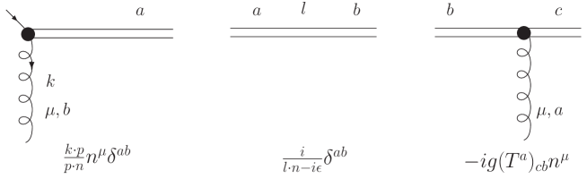
Figure 1: Feynman rules for the eikonal line, which is represented by a double line. $a,b$ and $c$ denote color indices.

The multiple scattering between the outgoing quark pair and the classical color field of the nucleus can be readily resummed to all orders [43, 44]. This gives rise to a path-ordered gauge factor along the straight line that extends in $x^{-}$ from minus infinity to plus infinity. More precisely, for a quark with incoming momentum $l$ and outgoing momentum $l+k$, the path-ordered gauge factor reads,

$$2\pi\delta(k^{-})p^{\mu}[U-1](k_{\perp})\,,$$ (3)

with

$$[U-1](k_{\perp})=\int d^{2}x_{\perp}e^{-ik_{\perp}\cdot x_{\perp}}[U(x_{\perp})-1]\,,$$ (4)

and

$$U(x_{\perp})=\langle{\cal P}e^{-ig_{s}\int_{-\infty}^{+\infty}dx^{-}A^{+}(x^{-},\ x_{\perp})}\rangle_{A}\,,$$ (5)

where $A^{+}=A^{+}_{c}t^{c}$ with $t^{c}$ being the generators in the fundamental representation. Similarly, multiple scattering between incoming gluon (or eikonal line) and classical color field of the nucleus also can be resummed to all orders,

$$2\pi\delta(k^{-})p^{\mu}[\tilde{U}-1](k_{\perp})\,,$$ (6)

with

$$[\tilde{U}-1](k_{\perp})=\int d^{2}x_{\perp}e^{-ik_{\perp}\cdot x_{\perp}}[\tilde{U}(x_{\perp})-1]\,,$$ (7)

and

$$\tilde{U}(x_{\perp})=\langle{\cal P}e^{-ig_{s}\int_{-\infty}^{+\infty}dx^{-}\tilde{A}^{+}(x^{-},\ x_{\perp})}\rangle_{A}\,,$$ (8)

where $(\tilde{A}^{+})_{ab}=A^{+}_{c}(-if^{abc})$ with $f^{abc}$ being the generators in the adjoint representation.

We use these as the building blocks to compute the amplitude for quark pair production in high energy $pA$ collisions. It is straightforward to obtain the production amplitude for diagram(a) illustrated in the Fig.2,

$${\cal M}^{(a)}=-ig_{s}\bar{u}(l_{1})\gamma^{\rho}t^{a}\frac{l\!\!\!/_{2}-k\!\!\!/_{1}-m}{(l_{2}-k_{1})^{2}-m^{2}+i\epsilon}p\!\!\!/[U^{\dagger}-1](k_{1\perp})v(l_{2})\frac{\varepsilon_{\rho\sigma}(k_{2})}{k^{2}_{2}+i\epsilon}n^{\sigma}\frac{k_{2}\!\cdot\!p}{p\!\cdot\!n}\phi_{p}(x_{2},k_{2\perp})\,,$$ (9)

where the factor $2\pi\delta(k_{1}^{-})$ is suppressed. $m$ is the quark mass. $k_{2}=l_{1}+l_{2}-k_{1}$ denotes the momentum of the gluon from the proton with $l_{1}$ and $l_{2}$ being the quark and anti-quark momentum, respectively. $\phi_{p}(x_{2},k_{2\perp})$ represents the probability amplitude for finding a gluon carrying a certain momentum inside the proton, with $x_{2}g(x_{2},k_{2\perp})=\phi_{p}\phi_{p}^{*}$. The other diagrams shown in Fig.2 give,

$${\cal M}^{(b)}\!\! = \!\!-ig_{s}\bar{u}(l_{1})p\!\!\!/[U-1](k_{1\perp})\frac{l\!\!\!/_{1}-k\!\!\!/_{1}+m}{(l_{1}-k_{1})^{2}-m^{2}+i\epsilon}\gamma^{\rho}t^{a}v(l_{2})\frac{\varepsilon_{\rho\sigma}(k_{2})}{k^{2}_{2}+i\epsilon}n^{\sigma}\frac{k_{2}\!\cdot\!p}{p\!\cdot\!n}\phi_{p}(x_{2},k_{2\perp})$$ (10)

$${\cal M}^{(c)}\!\! = \!\!g_{s}\!\!\int\!\frac{d^{4}k_{1}^{\prime}}{(2\pi)^{3}}\delta(k_{1}^{{}^{\prime}-})\bar{u}(l_{1})p\!\!\!/[U-1](k_{1\perp}-k_{1\perp}^{\prime})\frac{l\!\!\!/_{1}-k\!\!\!/_{1}+k\!\!\!/_{1}^{\prime}+m}{(l_{1}-k_{1}+k_{1}^{\prime})^{2}-m^{2}+i\epsilon}\gamma^{\rho}t^{a}$$ (11)

$$\ \ \ \ \ \ \ \ \ \ \ \ \ \times\frac{l\!\!\!/_{2}-k\!\!\!/_{1}^{\prime}-m}{(l_{2}-k_{1}^{\prime})^{2}-m^{2}+i\epsilon}p\!\!\!/[U^{\dagger}-1](k_{1\perp}^{\prime})v(l_{2})\frac{\varepsilon_{\rho\sigma}(k_{2})}{k^{2}_{2}+i\epsilon}n^{\sigma}\frac{k_{2}\!\cdot\!p}{p\!\cdot\!n}\phi_{p}(x_{2},k_{2\perp})$$

$${\cal M}^{(d)}\!\! = \!\!-ig_{s}\bar{u}(l_{1})\gamma^{\rho}t^{b}v(l_{2})\frac{1}{k_{1}\!\cdot\!n-i\epsilon}\frac{\varepsilon_{\rho\sigma}(k_{2}+k_{1})}{(k_{2}+k_{1})^{2}+i\epsilon}n^{\sigma}\frac{(k_{2}+k_{1})\!\cdot\!p}{p\!\cdot\!n}[\tilde{U}-1]_{ba}(k_{1\perp})\phi_{p}(x_{2},k_{2\perp})$$ (12)

$${\cal M}^{(e)}\!\! = \!\!-ig_{s}\bar{u}(l_{1})\gamma^{\rho}t^{b}v(l_{2})\frac{\varepsilon_{\rho\rho^{\prime}}(k_{2}+k_{1})}{(k_{2}+k_{1})^{2}+i\epsilon}\frac{\varepsilon_{\sigma\sigma^{\prime}}(k_{2})}{k_{2}^{2}+i\epsilon}p^{\mu}\Lambda^{\mu\rho^{\prime}\sigma^{\prime}}n^{\sigma}\frac{k_{2}\!\cdot\!p}{p\!\cdot\!n}[\tilde{U}-1]_{ba}(k_{1\perp})\phi_{p}(x_{2},k_{2\perp})\ .$$ (13)

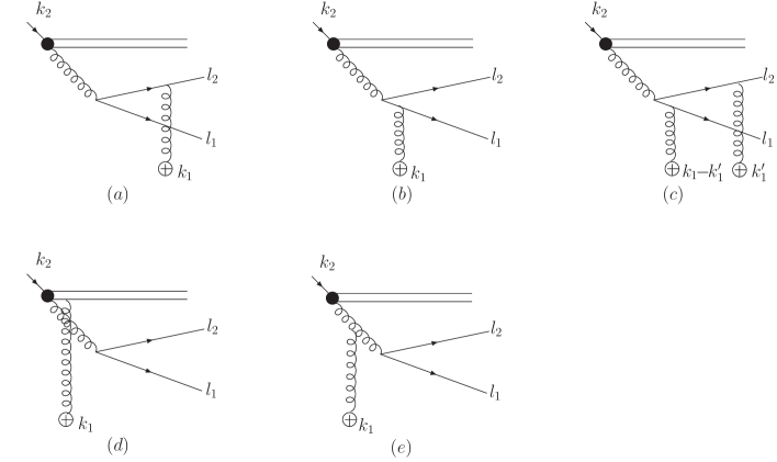
Figure 2: The diagrams contributing to quark pair production. The gluon line terminated by a $\oplus$ denotes a classical field insertion. The contributions from all other diagrams disappear because the multiple poles are located in the same half plane.

Putting all these terms together, we obtain the following expression for the complete production amplitude,

$${\cal M} = {\cal M}^{(a)}+{\cal M}^{(b)}+{\cal M}^{(c)}+{\cal M}^{(d)}+{\cal M}^{(e)}$$ (14)

$$= \!\!g_{s}\!\!\int\!\frac{d^{4}k_{1}^{\prime}}{(2\pi)^{3}}\left\{\delta(k_{1}^{{}^{\prime}-})\bar{u}(l_{1})p\!\!\!/\frac{l\!\!\!/_{1}-k\!\!\!/_{1}+k\!\!\!/_{1}^{\prime}+m}{(l_{1}-k_{1}+k_{1}^{\prime})^{2}-m^{2}+i\epsilon}\gamma^{\rho}\frac{l\!\!\!/_{2}-k\!\!\!/_{1}^{\prime}-m}{(l_{2}-k_{1}^{\prime})^{2}-m^{2}+i\epsilon}p\!\!\!/\right.\$$

$$\!\!\!\left.\ \times\left[U(k_{1\perp}-k_{1\perp}^{\prime})t^{a}U^{\dagger}(k_{1\perp}^{\prime})\right]v(l_{2})\frac{\varepsilon_{\rho\sigma}(k_{2})}{k^{2}_{2}+i\epsilon}n^{\sigma}\frac{k_{2}\!\cdot\!p}{p\!\cdot\!n}\phi_{p}(x_{2},k_{2\perp})\right\}-ig_{s}\bar{u}(l_{1})\gamma^{\rho}t^{b}v(l_{2})\tilde{U}_{ba}(k_{1\perp})$$

$$\times\left[\frac{\varepsilon_{\rho\rho^{\prime}}(k_{2}+k_{1})}{(k_{2}+k_{1})^{2}+i\epsilon}\frac{\varepsilon_{\sigma\sigma^{\prime}}(k_{2})}{k_{2}^{2}+i\epsilon}p^{\mu}\Lambda^{\mu\rho^{\prime}\sigma^{\prime}}+\frac{1}{k_{1}\!\cdot\!n-i\epsilon}\frac{\varepsilon_{\rho\sigma}(k_{2}+k_{1})}{(k_{2}+k_{1})^{2}+i\epsilon}\right]n^{\sigma}\frac{k_{2}\!\cdot\!p}{p\!\cdot\!n}\phi_{p}(x_{2},k_{2\perp})\ .$$

To arrive the above formula, we have made use of the Dirac equation of motion obeyed by the free spinors and the following identity for the Wilson lines in the different representations:

$$U(x_{\perp})t^{a}U^{\dagger}(x_{\perp})=t^{b}\tilde{U}^{ba}(x_{\perp})\ .$$ (15)

After some algebra, this production amplitude can be further rewritten in a more conventional form,

$${\cal M} = \!\!ig_{s}\frac{k_{2}\!\cdot\!p}{k^{2}_{2}}\phi_{p}(x_{2},k_{2\perp})$$ (16)

$$\times\bar{u}(l_{1})\left\{T_{g}(k_{1\perp})t^{b}\tilde{U}_{ba}(k_{1\perp})+\!\int\!\frac{d^{2}k_{1\perp}^{\prime}}{(2\pi)^{2}}\left[T_{q\bar{q}}(k_{1\perp},k_{1\perp}^{\prime})U(k_{1\perp}-k_{1\perp}^{\prime})t^{a}U^{\dagger}(k_{1\perp}^{\prime})\right]\right\}v(l_{2})$$

where,

$$T_{q\bar{q}}(k_{2\perp},k_{1\perp},k_{1\perp}^{\prime})\!\!\! = \!\!\!i\int\frac{dk^{{}^{\prime}-}dk^{{}^{\prime}+}}{2\pi}\delta(k_{1}^{{}^{\prime}-})p\!\!\!/\frac{l\!\!\!/_{1}-k\!\!\!/_{1}+k\!\!\!/_{1}^{\prime}+m}{(l_{1}-k_{1}+k_{1}^{\prime})^{2}-m^{2}+i\epsilon}n\!\!\!/\frac{l\!\!\!/_{2}-k\!\!\!/_{1}^{\prime}-m}{(l_{2}-k_{1}^{\prime})^{2}-m^{2}+i\epsilon}p\!\!\!/$$ (17)

$$T_{g}(k_{2\perp},k_{1\perp})\!\!\! = \!\!\!\frac{1}{(k_{1}+k_{2})^{2}}\left[\frac{k_{1\perp}^{2}-(k_{1\perp}+k_{2\perp})^{2}}{k_{2}\cdot p}p\!\!\!/-\frac{k_{2\perp}^{2}}{k_{1}\cdot n}n\!\!\!/+2k\!\!\!/_{2\perp}\right]-\frac{1}{k_{2}\cdot p}p\!\!\!/\ .$$ (18)

This result is in agreement with the production amplitude obtained in Ref. [19] up to a trivial prefactor. Note that $T_{q\bar{q}}(k_{2\perp}=0,k_{1\perp},k_{1\perp}^{\prime})+T_{g}(k_{2\perp}=0,k_{1\perp})=0$.

Squaring the amplitude, we obtain the following expression for the pair production cross section,

$$\frac{d\sigma}{d{\cal P.S.}} = \frac{\alpha_{s}\pi}{N_{c}^{2}-1}\int\frac{2d^{2}k_{1\perp}}{(2\pi)^{3}}d^{2}k_{2\perp}\frac{d^{2}k_{1\perp}^{\prime}d^{2}k_{1\perp}^{\prime\prime}}{(2\pi)^{4}}\frac{1}{(2\pi)^{2}}\delta^{2}(k_{1\perp}+k_{2\perp}-q_{\perp})x_{2}g(x_{2},k_{2\perp})$$ (19)

$$\times \!\!\!\int d^{2}x_{\perp}d^{2}y_{\perp}d^{2}x_{\perp}^{\prime}d^{2}y_{\perp}^{\prime}e^{-ix_{\perp}\cdot(k_{1\perp}-k_{1\perp}^{\prime})}e^{-iy_{\perp}\cdot k_{1\perp}^{\prime}}e^{ix_{\perp}^{\prime}\cdot(k_{1\perp}-k_{1\perp}^{\prime\prime})}e^{iy_{\perp}^{\prime}\cdot k_{1\perp}^{\prime\prime}}\frac{1}{k_{2\perp}^{2}}$$

$$\!\!\!\times\left\{{\rm Tr}\left[(l\!\!\!/_{1}+m)T_{q\bar{q}}(l\!\!\!/_{2}-m)\gamma^{0}T_{q\bar{q}}^{{\dagger}^{\prime}}\gamma^{0}\right]C(x_{\perp},y_{\perp},y_{\perp}^{\prime},x_{\perp}^{\prime})\right.\$$

$$\left.\ +{\rm Tr}\left[(l\!\!\!/_{1}+m)T_{q\bar{q}}(l\!\!\!/_{2}-m)\gamma^{0}T_{g}^{{\dagger}^{\prime}}\gamma^{0}\right]C(x_{\perp},y_{\perp},y_{\perp}^{\prime},y_{\perp}^{\prime})\right.\$$

$$\left.\ +{\rm Tr}\left[(l\!\!\!/_{1}+m)T_{g}(l\!\!\!/_{2}-m)\gamma^{0}T_{q\bar{q}}^{{\dagger}^{\prime}}\gamma^{0}\right]C(x_{\perp},x_{\perp},y_{\perp}^{\prime},x_{\perp}^{\prime})\right.\$$

$$\left.\ +{\rm Tr}\left[(l\!\!\!/_{1}+m)T_{g}(l\!\!\!/_{2}-m)\gamma^{0}T_{g}^{{\dagger}^{\prime}}\gamma^{0}\right]C(x_{\perp},x_{\perp},y_{\perp}^{\prime},y_{\perp}^{\prime})\right\}\ .$$

where $g(x_{2},k_{2\perp})$ denotes the un-integrated gluon distribution of a proton. In the phase space factor $d{\cal P.S.}=d^{2}l_{1\perp}d^{2}l_{2\perp}dy_{1}dy_{2}$, the quantities $y_{1},y_{2}$ are the rapidities of the produced quark and anti-quark respectively. The quark pair imbalance is defined as $q_{\perp}=l_{1\perp}+l_{2\perp}$. The factor $2/(2\pi)^{3}$ associated with the phase space integration is chosen such that for a single gluon target, $\int\frac{2d^{2}k_{1\perp}}{(2\pi)^{3}}\frac{k_{1\perp}^{2}}{g^{2}N_{c}}\langle\tilde{U}(k_{1\perp})\tilde{U}^{\dagger}(k_{1\perp})\rangle_{\rm gluon}=x_{1}\delta(1-x_{1})$ at lowest non-trivial order (see, for example, Ref. [45]). To obtain the above result, we have defined the normalization factor and the flux factor to be $k_{2\perp}^{2}/(2k_{2}\cdot p(N_{c}^{2}-1))$ and $1/(2k_{2}\cdot p)$, respectively, rather than $k_{1\perp}^{2}k_{2\perp}^{2}/(4x_{1}x_{2}P_{A}\cdot P_{B}(N_{c}^{2}-1)^{2})$, $1/(4x_{1}x_{2}P_{A}\cdot P_{B})$ as used in Ref. [16], since the Lipatov approximation is only applied on the proton side. We have omitted the arguments of $T_{q\bar{q}},T_{g}$. And $T_{q\bar{q}}^{\prime},T_{g}^{\prime}$ denote the same quantities with $k_{1\perp}^{\prime}$ replaced by $k_{1\perp}^{\prime\prime}$. The four point function $C(x_{\perp},y_{\perp},y_{\perp}^{\prime},x_{\perp}^{\prime})$ is defined as,

$$C(x_{\perp},y_{\perp},y_{\perp}^{\prime},x_{\perp}^{\prime})={\rm Tr_{c}}\left\langle U(x_{\perp})t^{a}U^{\dagger}(y_{\perp})U(y_{\perp}^{\prime})t^{a}U^{\dagger}(x_{\perp}^{\prime})\right\rangle_{x_{1}}\,$$ (20)

Here ${\rm Tr_{c}}$ is a trace over the color indices. The longitudinal momentum fraction of proton and nucleus carried by the incoming gluons are constrained by the kinematics,

$$x_{1}=\frac{|l_{1\perp}|e^{-y_{1}}+|l_{2\perp}|e^{-y_{2}}}{\sqrt{s}}\ \ \ ,\ \ x_{2}=\frac{|l_{1\perp}|e^{y_{1}}+|l_{2\perp}|e^{y_{2}}}{\sqrt{s}}\ ,$$ (21)

where $\sqrt{s}$ is the center of mass energy.

With this derived full CGC result, we proceed to the correlation limit where $|P_{\perp}|\equiv|l_{1\perp}-l_{2\perp}|/2\gg|q_{\perp}|/2$. In this kinematical region, we may systemically neglect the terms suppressed by powers of $|k_{2\perp}|/|P_{\perp}|,|k_{1\perp}|/|P_{\perp}|$, $|k_{1\perp}^{\prime}|/|P_{\perp}|$ and $|k_{1\perp}^{\prime\prime}|/|P_{\perp}|$ in the four hard coefficients. We first perform a Taylor expansion of the hard coefficients in terms of $k_{2\perp}$. By dropping all terms suppressed by powers of $|k_{2\perp}|/|P_{\perp}|$, one ends up with,

$$\frac{d\sigma}{d{\cal P.S.}} \approx \frac{\alpha_{s}}{N_{c}^{2}-1}\int\frac{d^{2}k_{1\perp}}{(2\pi)^{4}}d^{2}k_{2\perp}\frac{d^{2}k_{1\perp}^{\prime}d^{2}k_{1\perp}^{\prime\prime}}{(2\pi)^{4}}\delta^{2}(k_{1\perp}+k_{2\perp}-q_{\perp})x_{2}g(x_{2},k_{2\perp})$$ (22)

$$\times \!\!\!\int d^{2}x_{\perp}d^{2}y_{\perp}d^{2}x_{\perp}^{\prime}d^{2}y_{\perp}^{\prime}e^{-ix_{\perp}\cdot(k_{1\perp}-k_{1\perp}^{\prime})}e^{-iy_{\perp}\cdot k_{1\perp}^{\prime}}e^{ix_{\perp}^{\prime}\cdot(k_{1\perp}-k_{1\perp}^{\prime\prime})}e^{iy_{\perp}^{\prime}\cdot k_{1\perp}^{\prime\prime}}$$

$$\!\!\!\times\left\{{\rm Tr}\left[(l\!\!\!/_{1}+m)\bar{T}_{q\bar{q}}(l\!\!\!/_{2}-m)\gamma^{0}\bar{T}_{q\bar{q}}^{{\dagger}^{\prime}}\gamma^{0}\right]_{k_{2\perp}=0}C(x_{\perp},y_{\perp},y_{\perp}^{\prime},x_{\perp}^{\prime})\right.\$$

$$\left.\ +{\rm Tr}\left[(l\!\!\!/_{1}+m)\bar{T}_{q\bar{q}}(l\!\!\!/_{2}-m)\gamma^{0}\bar{T}_{g}^{{\dagger}^{\prime}}\gamma^{0}\right]_{k_{2\perp}=0}C(x_{\perp},y_{\perp},y_{\perp}^{\prime},y_{\perp}^{\prime})\right.\$$

$$\left.\ +{\rm Tr}\left[(l\!\!\!/_{1}+m)\bar{T}_{g}(l\!\!\!/_{2}-m)\gamma^{0}\bar{T}_{q\bar{q}}^{{\dagger}^{\prime}}\gamma^{0}\right]_{k_{2\perp}=0}C(x_{\perp},x_{\perp},y_{\perp}^{\prime},x_{\perp}^{\prime})\right.\$$

$$\left.\ +{\rm Tr}\left[(l\!\!\!/_{1}+m)\bar{T}_{g}(l\!\!\!/_{2}-m)\gamma^{0}\bar{T}_{g}^{{\dagger}^{\prime}}\gamma^{0}\right]_{k_{2\perp}=0}C(x_{\perp},x_{\perp},y_{\perp}^{\prime},y_{\perp}^{\prime})\right\}\ ,$$

and with $\bar{T}_{q\bar{q}},\bar{T}_{g}$ given by,

$$\bar{T}_{q\bar{q}}(k_{1\perp},k_{1\perp}^{\prime})\!\!\! = \!\!\!i\int\frac{dk^{{}^{\prime}-}dk^{{}^{\prime}+}}{2\pi}\delta(k_{1}^{{}^{\prime}-})p\!\!\!/\frac{l\!\!\!/_{1}-k\!\!\!/_{1}+k\!\!\!/_{1}^{\prime}+m}{(l_{1}-k_{1}+k_{1}^{\prime})^{2}-m^{2}+i\epsilon}\frac{\hat{k}\!\!\!/_{2\perp}}{(k_{2}\cdot p)}\frac{l\!\!\!/_{2}-k\!\!\!/_{1}^{\prime}-m}{(l_{2}-k_{1}^{\prime})^{2}-m^{2}+i\epsilon}p\!\!\!/$$ (23)

$$\bar{T}_{g}(k_{1\perp})\!\!\! = \!\!\!\frac{1}{(k_{1}+x_{2}P_{B})^{2}}\left[\frac{-2k_{1\perp}\cdot\hat{k}_{2\perp}}{k_{2}\cdot p}p\!\!\!/+2\hat{k}\!\!\!/_{2\perp}\right]\ ,$$ (24)

where $\hat{k}_{2\perp}=k_{2\perp}/|k_{2\perp}|$ is a unit vector.

Now let’s move on to discuss the power expansion on the nucleus side. The fact that the integrations over $k_{1\perp}^{\prime},k_{1\perp}^{\prime\prime}$ are dominated by the kinematical region $|k_{1\perp}^{\prime}|\sim|k_{1\perp}^{\prime\prime}|\sim Q_{s}$ — because the typical small $x$ gluon transverse momentum is characterized by the saturation momentum — allows us to employ the power expansion in the correlation limit $Q_{s}\sim|k_{1\perp}+k_{2\perp}|/2\ll|P_{\perp}|$. To facilitate the power expansion, we replace $\bar{T}_{q\bar{q}}(k_{1\perp},k_{1\perp}^{\prime})$, $\bar{T}_{g}(k_{1\perp})$ with the following two expressions with the help of Ward identities (gauge invariance violation terms in the amplitude are proportional to the gluon off-shellness $\sim k_{1\perp}^{2}$ , and thus can be neglected in the correlation limit.),

$$\!\!\!\!\!\!\!\!\!\!\!\!\!\!\!\!\!\!\!\!\bar{T}_{q\bar{q}}(k_{1\perp},k_{1\perp}^{\prime})\Rightarrow\bar{T}_{q\bar{q}}(k_{1\perp},k_{1\perp}^{\prime})$$ (26)

$$\!\!\!\!\!\!-i\int\frac{dk^{{}^{\prime}-}dk^{{}^{\prime}+}}{2\pi}\delta(k_{1}^{{}^{\prime}-})\frac{k\!\!\!/_{1}-k\!\!\!/_{1}^{\prime}}{(x_{1}-x_{1}^{\prime})P_{A}^{+}}\frac{l\!\!\!/_{1}-k\!\!\!/_{1}+k\!\!\!/_{1}^{\prime}+m}{(l_{1}-k_{1}+k_{1}^{\prime})^{2}-m^{2}+i\epsilon}\frac{\hat{k}\!\!\!/_{2\perp}}{(k_{2}\cdot p)}\frac{l\!\!\!/_{2}-k\!\!\!/_{1}^{\prime}-m}{(l_{2}-k_{1}^{\prime})^{2}-m^{2}+i\epsilon}\frac{k\!\!\!/_{1}^{\prime}}{x_{1}^{\prime}P_{A}^{+}}$$

$$\Rightarrow -\left[\frac{\gamma_{i}}{x_{1}P_{A}^{+}}\frac{l\!\!\!/_{1}-k\!\!\!/_{1}+m}{(l_{1}-k_{1})^{2}-m^{2}+i\epsilon}\frac{\hat{k}\!\!\!/_{2\perp}}{(k_{2}\cdot p)}\right]_{k_{1\perp}=0}(k_{1\perp}^{i}-k_{1\perp}^{\prime i})$$

$$-\left[\frac{\hat{k}\!\!\!/_{2\perp}}{(k_{2}\cdot p)}\frac{l\!\!\!/_{2}-k\!\!\!/_{1}-m}{(l_{2}-k_{1})^{2}-m^{2}+i\epsilon}\frac{\gamma_{i}}{x_{1}P_{A}^{+}}\right]_{k_{1\perp}=0}k_{1\perp}^{\prime i}+O(\frac{k_{1\perp}^{2}}{P_{\perp}^{2}})\approx\tilde{T}_{q\bar{q},i}^{A}(k_{1\perp}^{i}-k_{1\perp}^{\prime i})+\tilde{T}_{q\bar{q},i}^{B}k_{1\perp}^{\prime i}$$

$$\!\!\!\!\!\!\!\!\!\!\!\!\!\!\!\!\!\!\!\!\bar{T}_{g}(k_{1\perp})\Rightarrow\bar{T}_{g}(k_{1\perp})-\frac{1}{(k_{1}+x_{2}P_{B})^{2}}\left(2+\frac{k_{1\perp}^{2}}{x_{1}x_{2}P_{A}^{+}P_{B}^{-}}\right)\hat{k}\!\!\!/_{2\perp}$$

$$\approx\left[\frac{1}{(k_{1}+x_{2}P_{B})^{2}}\frac{-2\hat{k}_{2\perp,i}}{k_{2}\cdot p}p\!\!\!/\right]_{k_{1\perp}=0}k_{1\perp}^{i}=\tilde{T}_{g,i}k_{1\perp}^{i}\ ,$$

with $i$ denoting the transverse index. By making the above replacement, the differential cross section can be rewritten in the form,

$$\frac{d\sigma}{d{\cal P.S.}} \approx \frac{\alpha_{s}}{(N_{c}^{2}-1)}\int\frac{d^{2}k_{1\perp}d^{2}k_{2\perp}}{(2\pi)^{4}}\delta^{2}(k_{1\perp}+k_{2\perp}-q_{\perp})x_{2}g(x_{2},k_{2\perp})\int d^{2}x_{\perp}d^{2}x_{\perp}^{\prime}e^{-ik_{1\perp}\cdot(x_{\perp}-x_{\perp}^{\prime})}$$ (27)

$$\!\!\!\times\left\{{\rm Tr}\left[(l\!\!\!/_{1}+m)\tilde{T}_{q\bar{q},i}^{A}(l\!\!\!/_{2}-m)\gamma^{0}\tilde{T}_{q\bar{q},j}^{A{\dagger}^{\prime}}\gamma^{0}\right]_{k_{2\perp},k_{1\perp}=0}\left[\frac{\partial^{2}C(x_{\perp},y_{\perp},y_{\perp}^{\prime},x_{\perp}^{\prime})}{\partial x_{\perp}^{i}\partial x_{\perp}^{\prime j}}\right]_{x_{\perp}=y_{\perp},x_{\perp}^{\prime}=y_{\perp}^{\prime}}\right.\$$

$$\left.\ +{\rm Tr}\left[(l\!\!\!/_{1}+m)\tilde{T}_{q\bar{q},i}^{A}(l\!\!\!/_{2}-m)\gamma^{0}\tilde{T}_{q\bar{q},j}^{B{\dagger}^{\prime}}\gamma^{0}\right]_{k_{2\perp},k_{1\perp}=0}\left[\frac{\partial^{2}C(x_{\perp},y_{\perp},y_{\perp}^{\prime},x_{\perp}^{\prime})}{\partial x_{\perp}^{i}\partial y_{\perp}^{\prime j}}\right]_{x_{\perp}=y_{\perp},x_{\perp}^{\prime}=y_{\perp}^{\prime}}\right.\$$

$$\left.\ +{\rm Tr}\left[(l\!\!\!/_{1}+m)\tilde{T}_{q\bar{q},i}^{B}(l\!\!\!/_{2}-m)\gamma^{0}\tilde{T}_{q\bar{q},j}^{A{\dagger}^{\prime}}\gamma^{0}\right]_{k_{2\perp},k_{1\perp}=0}\left[\frac{\partial^{2}C(x_{\perp},y_{\perp},y_{\perp}^{\prime},x_{\perp}^{\prime})}{\partial y_{\perp}^{i}\partial x_{\perp}^{\prime j}}\right]_{x_{\perp}=y_{\perp},x_{\perp}^{\prime}=y_{\perp}^{\prime}}\right.\$$

$$\left.\ +{\rm Tr}\left[(l\!\!\!/_{1}+m)\tilde{T}_{q\bar{q},i}^{B}(l\!\!\!/_{2}-m)\gamma^{0}\tilde{T}_{q\bar{q},j}^{B{\dagger}^{\prime}}\gamma^{0}\right]_{k_{2\perp},k_{1\perp}=0}\left[\frac{\partial^{2}C(x_{\perp},y_{\perp},y_{\perp}^{\prime},x_{\perp}^{\prime})}{\partial y_{\perp}^{i}\partial y_{\perp}^{\prime j}}\right]_{x_{\perp}=y_{\perp},x_{\perp}^{\prime}=y_{\perp}^{\prime}}\right.\$$

$$\left.\ +{\rm Tr}\left[(l\!\!\!/_{1}+m)\tilde{T}_{q\bar{q},i}^{A}(l\!\!\!/_{2}-m)\gamma^{0}\tilde{T}_{g,j}^{{\dagger}^{\prime}}\gamma^{0}\right]_{k_{2\perp},k_{1\perp}=0}\left[\frac{\partial^{2}C(x_{\perp},y_{\perp},x_{\perp}^{\prime},x_{\perp}^{\prime})}{\partial x_{\perp}^{i}\partial x_{\perp}^{\prime j}}\right]_{x_{\perp}=y_{\perp}}\right.\$$

$$\left.\ +{\rm Tr}\left[(l\!\!\!/_{1}+m)\tilde{T}_{q\bar{q},i}^{B}(l\!\!\!/_{2}-m)\gamma^{0}\tilde{T}_{g,j}^{{\dagger}^{\prime}}\gamma^{0}\right]_{k_{2\perp},k_{1\perp}=0}\left[\frac{\partial^{2}C(x_{\perp},y_{\perp},x_{\perp}^{\prime},x_{\perp}^{\prime})}{\partial y_{\perp}^{i}\partial x_{\perp}^{\prime j}}\right]_{x_{\perp}=y_{\perp}}\right.\$$

$$\left.\ +{\rm Tr}\left[(l\!\!\!/_{1}+m)\tilde{T}_{g,i}(l\!\!\!/_{2}-m)\gamma^{0}\tilde{T}_{q\bar{q},j}^{A{\dagger}^{\prime}}\gamma^{0}\right]_{k_{2\perp},k_{1\perp}=0}\left[\frac{\partial^{2}C(x_{\perp},x_{\perp},y_{\perp}^{\prime},x_{\perp}^{\prime})}{\partial x_{\perp}^{i}\partial x_{\perp}^{\prime j}}\right]_{x_{\perp}^{\prime}=y_{\perp}^{\prime}}\right.\$$

$$\left.\ +{\rm Tr}\left[(l\!\!\!/_{1}+m)\tilde{T}_{g,i}(l\!\!\!/_{2}-m)\gamma^{0}\tilde{T}_{q\bar{q},j}^{B{\dagger}^{\prime}}\gamma^{0}\right]_{k_{2\perp},k_{1\perp}=0}\left[\frac{\partial^{2}C(x_{\perp},x_{\perp},y_{\perp}^{\prime},x_{\perp}^{\prime})}{\partial x_{\perp}^{i}\partial y_{\perp}^{\prime j}}\right]_{x_{\perp}^{\prime}=y_{\perp}^{\prime}}\right.\$$

$$\left.\ +{\rm Tr}\left[(l\!\!\!/_{1}+m)\tilde{T}_{g,i}(l\!\!\!/_{2}-m)\gamma^{0}\tilde{T}_{g,j}^{{\dagger}^{\prime}}\gamma^{0}\right]_{k_{2\perp},k_{1\perp}=0}\left[\frac{\partial^{2}C(x_{\perp},x_{\perp},x_{\perp}^{\prime},x_{\perp}^{\prime})}{\partial x_{\perp}^{i}\partial x_{\perp}^{\prime j}}\right]\right\}\ ,$$

where the transverse momenta $k_{1\perp}^{\prime}$ and $k_{1\perp}^{\prime\prime}$ have been integrated out. As a result, the four point functions collapse into the two point functions. The calculation of the Dirac traces in the above formula is rather easy, while the evaluation of the soft part in the McLerran-Venugopalan(MV) model is a bit more involved. In general, the tensor structure of the soft part can be decomposed in the following way,

$$\int\left[\frac{\partial^{2}C(x_{\perp},y_{\perp},y_{\perp}^{\prime},x_{\perp}^{\prime})}{\partial x_{\perp,i}\partial x_{\perp,j}^{\prime}}\right]_{x_{\perp}=y_{\perp},x_{\perp}^{\prime}=y_{\perp}^{\prime}}=\frac{\delta_{\perp}^{ij}}{2}\,F_{1}(x_{1},k_{1\perp})+\bigg{(}\hat{k}_{1\perp}^{i}\hat{k}_{1\perp}^{j}-\frac{1}{2}\delta_{\perp}^{ij}\bigg{)}H_{1}(x_{1},k_{1\perp})\,.$$ (28)

where $\int$ denotes $\int d^{2}x_{\perp}d^{2}x_{\perp}^{\prime}e^{-ik_{1\perp}\cdot(x_{\perp}-x_{\perp}^{\prime})}$. $\hat{k}_{1\perp}^{i}$ is a unit vector $\hat{k}_{1\perp}^{i}\equiv k_{1\perp}^{i}/|k_{1\perp}|$, and $\delta_{\perp}^{ij}=-g^{ij}+(p^{i}n^{j}+p^{j}n^{i})/p\cdot n$. The four point function $C(x_{\perp},y_{\perp},y_{\perp}^{\prime},x_{\perp}^{\prime})$ has been evaluated in the MV model in Ref. [19]. With the derived four point function, the coefficients $F_{i}$ and $H_{i}$ can be computed in a tedious but straightforward way. One finds,

$$F_{1} = \int\left[\frac{\partial^{2}C(x_{\perp},y_{\perp},y_{\perp}^{\prime},x_{\perp}^{\prime})}{\partial x_{\perp}^{i}\partial x_{\perp}^{\prime j}}\right]_{x_{\perp}=y_{\perp},x_{\perp}^{\prime}=y_{\perp}^{\prime}}\!\!\!\!\!\!\!\delta_{\perp}^{ij}=\int\left[\frac{\partial^{2}C(x_{\perp},y_{\perp},y_{\perp}^{\prime},x_{\perp}^{\prime})}{\partial y_{\perp}^{i}\partial y_{\perp}^{\prime j}}\right]_{x_{\perp}=y_{\perp},x_{\perp}^{\prime}=y_{\perp}^{\prime}}\!\!\!\!\!\!\!\delta_{\perp}^{ij}$$ (29)

$$F_{2} = \int\left[\frac{\partial^{2}C(x_{\perp},y_{\perp},y_{\perp}^{\prime},x_{\perp}^{\prime})}{\partial x_{\perp}^{i}\partial y_{\perp}^{\prime j}}\right]_{x_{\perp}=y_{\perp},x_{\perp}^{\prime}=y_{\perp}^{\prime}}\!\!\!\!\!\!\!\delta_{\perp}^{ij}=\int\left[\frac{\partial^{2}C(x_{\perp},y_{\perp},y_{\perp}^{\prime},x_{\perp}^{\prime})}{\partial y_{\perp}^{i}\partial y_{\perp}^{\prime j}}\right]_{x_{\perp}=y_{\perp},x_{\perp}^{\prime}=y_{\perp}^{\prime}}\!\!\!\!\!\!\!\delta_{\perp}^{ij}$$ (30)

$$F_{3} = \int\left[\frac{\partial^{2}C(x_{\perp},x_{\perp},y_{\perp}^{\prime},x_{\perp}^{\prime})}{\partial x_{\perp}^{i}\partial x_{\perp}^{\prime j}}\right]_{x_{\perp}^{\prime}=y_{\perp}^{\prime}}\delta_{\perp}^{ij}=\int\left[\frac{\partial^{2}C(x_{\perp},x_{\perp},y_{\perp}^{\prime},x_{\perp}^{\prime})}{\partial y_{\perp}^{i}\partial x_{\perp}^{\prime j}}\right]_{x_{\perp}^{\prime}=y_{\perp}^{\prime}}\delta_{\perp}^{ij}$$ (31)

$$= \int\left[\frac{\partial^{2}C(x_{\perp},y_{\perp},x_{\perp}^{\prime},x_{\perp}^{\prime})}{\partial y_{\perp}^{i}\partial x_{\perp}^{\prime j}}\right]_{x_{\perp}=y_{\perp}}\delta_{\perp}^{ij}=\int\left[\frac{\partial^{2}C(x_{\perp},y_{\perp},x_{\perp}^{\prime},x_{\perp}^{\prime})}{\partial y_{\perp}^{i}\partial x_{\perp}^{\prime j}}\right]_{x_{\perp}=y_{\perp}}\delta_{\perp}^{ij}$$

$$= \frac{1}{2}\int\left[\frac{\partial^{2}C(x_{\perp},x_{\perp},x_{\perp}^{\prime},x_{\perp}^{\prime})}{\partial x_{\perp}^{i}\partial x_{\perp}^{\prime j}}\right]\delta_{\perp}^{ij}\ ,$$

and,

$$H_{1} = \int\left[\frac{\partial^{2}C(x_{\perp},y_{\perp},y_{\perp}^{\prime},x_{\perp}^{\prime})}{\partial x_{\perp,i}\partial x_{\perp,j}^{\prime}}\right]_{x_{\perp}=y_{\perp},x_{\perp}^{\prime}=y_{\perp}^{\prime}}\bigg{(}2\hat{k}_{1\perp}^{i}\hat{k}_{1\perp}^{j}-\delta_{\perp}^{ij}\bigg{)}$$ (32)

$$= \int\left[\frac{\partial^{2}C(x_{\perp},y_{\perp},y_{\perp}^{\prime},x_{\perp}^{\prime})}{\partial y_{\perp}^{i}\partial y_{\perp}^{\prime j}}\right]_{x_{\perp}=y_{\perp},x_{\perp}^{\prime}=y_{\perp}^{\prime}}\bigg{(}2\hat{k}_{1\perp}^{i}\hat{k}_{1\perp}^{j}-\delta_{\perp}^{ij}\bigg{)}$$

$$H_{2} = \int\left[\frac{\partial^{2}C(x_{\perp},y_{\perp},y_{\perp}^{\prime},x_{\perp}^{\prime})}{\partial x_{\perp}^{i}\partial y_{\perp}^{\prime j}}\right]_{x_{\perp}=y_{\perp},x_{\perp}^{\prime}=y_{\perp}^{\prime}}\bigg{(}2\hat{k}_{1\perp}^{i}\hat{k}_{1\perp}^{j}-\delta_{\perp}^{ij}\bigg{)}$$ (33)

$$= \int\left[\frac{\partial^{2}C(x_{\perp},y_{\perp},y_{\perp}^{\prime},x_{\perp}^{\prime})}{\partial y_{\perp}^{i}\partial y_{\perp}^{\prime j}}\right]_{x_{\perp}=y_{\perp},x_{\perp}^{\prime}=y_{\perp}^{\prime}}\bigg{(}2\hat{k}_{1\perp}^{i}\hat{k}_{1\perp}^{j}-\delta_{\perp}^{ij}\bigg{)}$$

$$H_{3} = \int\left[\frac{\partial^{2}C(x_{\perp},x_{\perp},y_{\perp}^{\prime},x_{\perp}^{\prime})}{\partial x_{\perp}^{i}\partial x_{\perp}^{\prime j}}\right]_{x_{\perp}^{\prime}=y_{\perp}^{\prime}}\bigg{(}2\hat{k}_{1\perp}^{i}\hat{k}_{1\perp}^{j}-\delta_{\perp}^{ij}\bigg{)}$$ (34)

$$= \int\left[\frac{\partial^{2}C(x_{\perp},x_{\perp},y_{\perp}^{\prime},x_{\perp}^{\prime})}{\partial y_{\perp}^{i}\partial x_{\perp}^{\prime j}}\right]_{x_{\perp}^{\prime}=y_{\perp}^{\prime}}\bigg{(}2\hat{k}_{1\perp}^{i}\hat{k}_{1\perp}^{j}-\delta_{\perp}^{ij}\bigg{)}$$

$$= \int\left[\frac{\partial^{2}C(x_{\perp},y_{\perp},x_{\perp}^{\prime},x_{\perp}^{\prime})}{\partial y_{\perp}^{i}\partial x_{\perp}^{\prime j}}\right]_{x_{\perp}=y_{\perp}}\bigg{(}2\hat{k}_{1\perp}^{i}\hat{k}_{1\perp}^{j}-\delta_{\perp}^{ij}\bigg{)}$$

$$= \int\left[\frac{\partial^{2}C(x_{\perp},y_{\perp},x_{\perp}^{\prime},x_{\perp}^{\prime})}{\partial y_{\perp}^{i}\partial x_{\perp}^{\prime j}}\right]_{x_{\perp}=y_{\perp}}\bigg{(}2\hat{k}_{1\perp}^{i}\hat{k}_{1\perp}^{j}-\delta_{\perp}^{ij}\bigg{)}$$

$$= \frac{1}{2}\int\left[\frac{\partial^{2}C(x_{\perp},x_{\perp},x_{\perp}^{\prime},x_{\perp}^{\prime})}{\partial x_{\perp}^{i}\partial x_{\perp}^{\prime j}}\right]\bigg{(}2\hat{k}_{1\perp}^{i}\hat{k}_{1\perp}^{j}-\delta_{\perp}^{ij}\bigg{)}\ ,$$

with,

$$F_{1} = 2\pi^{4}N_{c}\alpha_{s}x_{1}\left[G_{DP}(x_{1},k_{1\perp})+\left(1-\frac{4}{N_{c}^{2}}\right)G_{q\bar{q}}(x_{1},k_{1\perp})+\frac{2}{N_{c}^{2}}G_{WW}(x_{1},k_{1\perp})\right]$$ (35)

$$F_{2} = 2\pi^{4}N_{c}\alpha_{s}x_{1}\left[G_{DP}(x_{1},k_{1\perp})-\left(1-\frac{4}{N_{c}^{2}}\right)G_{q\bar{q}}(x_{1},k_{1\perp})-\frac{2}{N_{c}^{2}}G_{WW}(x_{1},k_{1\perp})\right]$$ (36)

$$F_{3} = 2\pi^{4}N_{c}\alpha_{s}x_{1}\left[2G_{DP}(x_{1},k_{1\perp})\right]$$ (37)

$$H_{1} = 2\pi^{4}N_{c}\alpha_{s}x_{1}\left[h_{1,DP}^{\perp g}(x_{1},k_{1\perp})+\left(1-\frac{4}{N_{c}^{2}}\right)h_{1,q\bar{q}}^{\perp g}(x_{1},k_{1\perp})+\frac{2}{N_{c}^{2}}h_{1,WW}^{\perp g}(x_{1},k_{1\perp})\right]$$ (38)

$$H_{2} = 2\pi^{4}N_{c}\alpha_{s}x_{1}\left[h_{1,DP}^{\perp g}(x_{1},k_{1\perp})-\left(1-\frac{4}{N_{c}^{2}}\right)h_{1,q\bar{q}}^{\perp g}(x_{1},k_{1\perp})-\frac{2}{N_{c}^{2}}h_{1,WW}^{\perp g}(x_{1},k_{1\perp})\right]$$ (39)

$$H_{3} = 2\pi^{4}N_{c}\alpha_{s}x_{1}\left[2h_{1,DP}^{\perp g}(x_{1},k_{1\perp})\right]\ .$$ (40)

To arrive at the results given above, we have neglected the logarithmic dependence of the saturation momentum on $r_{\perp}^{2}$. $G_{DP},G_{WW},h_{1,DP}^{\perp g}$ and $h_{1,WW}^{\perp g}$ are the unpolarized gluon dipole distribution, the Weizsäcker-Williams (WW) type unpolarized gluon distribution, the dipole type linearly polarized gluon distribution, and the WW type linearly polarized gluon distribution, respectively. In the MV model, they read [46, 47, 31],

$$x_{1}G_{DP}(x_{1},k_{1\perp})\!\!\! = \!\!\!x_{1}h^{\perp g}_{1,DP}(x_{1},k_{1\perp})=\frac{C_{F}S_{\perp}}{2\pi^{2}\alpha_{s}}k_{1\perp}^{2}\int\frac{d^{2}r_{\perp}}{(2\pi)^{2}}\,e^{-ik_{1\perp}\cdot r_{\perp}}e^{-\frac{r_{\perp}^{2}Q_{s}^{2}}{4}}$$ (41)

$$x_{1}G_{WW}(x_{1},k_{1\perp})\!\!\! = \!\!\!\frac{N_{c}^{2}-1}{N_{c}}\frac{S_{\perp}}{4\pi^{4}\alpha_{s}}\int d^{2}r_{\perp}e^{-ik_{1\perp}\cdot r_{\perp}}\,\frac{1}{r_{\perp}^{2}}\bigg{(}1-e^{-\frac{r_{\perp}^{2}Q_{s}^{2}}{4}}\bigg{)}$$ (42)

$$x_{1}h^{\perp g}_{1,WW}(x_{1},k_{1\perp})\!\!\! = \!\!\!\frac{N_{c}^{2}-1}{8\pi^{3}}\,S_{\perp}\int dr_{\perp}\,\frac{J_{2}(|k_{1\perp}||r_{\perp})|}{\frac{1}{4\mu_{A}}|r_{\perp}|Q_{s}^{2}}\bigg{(}1-e^{-\frac{r_{\perp}^{2}Q_{s}^{2}}{4}}\bigg{)}\,.$$ (43)

Here $S_{\perp}$ is the transverse area of the target nucleus. $Q_{s}^{2}=\alpha_{s}N_{c}\mu_{A}{\rm ln}\left[1/(r_{\perp}^{2}\Lambda_{QCD}^{2})\right]$ is the gluon saturation scale with $\mu_{A}$ being a common CGC parameter. $J_{2}$ is the second order Bessel function. Note that our convention for $h^{\perp g}_{1,WW}$ differs from that in Ref. [31] by a factor 1/2. The WW type gluon distributions have a clear physical interpretation as the number density of gluons inside a hadron/nucleus, while the dipole type distribution does not. On the other hand, the dipole type unpolarized gluon distribution in the adjoint representation enters the single gluon production cross section in pA collisions [48]. Besides these widely used gluon TMDs, two novel ones are given by,

$$x_{1}G_{q\bar{q}}(x_{1},k_{1\perp})\!\!\! = \!\!\!\frac{C_{F}S_{\perp}}{2\pi^{2}\alpha_{s}}\int\frac{d^{2}r_{\perp}}{(2\pi)^{2}}\,e^{-ik_{1\perp}\cdot r_{\perp}}\,Q_{s}^{2}e^{-\frac{r_{\perp}^{2}Q_{s}^{2}}{4}}\ ,$$ (44)

$$x_{1}h^{\perp g}_{1,q\bar{q}}(x_{1},k_{1\perp})\!\!\! = \!\!\!\frac{N_{c}^{2}-1}{8\pi^{3}}\,S_{\perp}\int d|r_{\perp}|\mu_{A}|r_{\perp}|J_{2}(|k_{1\perp}||r_{\perp}|)e^{-\frac{r_{\perp}^{2}Q_{s}^{2}}{4}}\,.$$ (45)

Collecting all the pieces together, the differential cross section for quark pair production can be written in the following general form,

$$\frac{d\sigma}{d{\cal P.S.}}=\frac{\alpha_{s}^{2}N_{c}}{\hat{s}^{2}(N_{c}^{2}-1)}\left[{\cal A}(q_{\perp}^{2})+\frac{m^{2}}{P_{\perp}^{2}}{\cal B}(q_{\perp}^{2})\cos 2\phi+{\cal C}(q_{\perp}^{2})\cos 4\phi\right]$$ (46)

where $\phi$ is the azimuthal angle between the transverse momenta $q_{\perp}$ and $P_{\perp}$. The coefficients ${\cal A}(q_{\perp}^{2})$, ${\cal B}(q_{\perp}^{2})$ and ${\cal C}(q_{\perp}^{2})$ contain convolutions of various gluon TMDs. Instead of presenting the full results for these coefficients, we neglect all higher powers in $m^{2}/P_{\perp}^{2}$ ,

$$\!\!\!\!\!\!\!\!\!\!\!\!\!\!{\cal A}(q_{\perp}^{2})=\int d^{2}k_{1\perp}d^{2}k_{2\perp}\delta^{2}(k_{1\perp}+k_{2\perp}-q_{\perp})x_{2}g(x_{2},k_{2\perp})\frac{(\hat{u}^{2}+\hat{t}^{2})}{4\hat{u}\hat{t}}$$

$$\times\left\{\frac{(\hat{t}-\hat{u})^{2}}{\hat{s}^{2}}x_{1}G_{DP}(x_{1},k_{1\perp})+x_{1}\left[\left(1-\frac{4}{N_{c}^{2}}\right)G_{q\bar{q}}(x_{1},k_{1\perp})+\frac{2}{N_{c}^{2}}G_{WW}(x_{1},k_{1\perp})\right]\right\}$$ (47)

$$\!\!\!\!\!\!\!\!\!\!\!\!\!\!{\cal B}(q_{\perp}^{2})=\int d^{2}k_{1\perp}d^{2}k_{2\perp}\delta^{2}(k_{1\perp}+k_{2\perp}-q_{\perp})x_{2}g(x_{2},k_{2\perp})$$

$$\times\left\{\left[2(\hat{k}_{1\perp}\cdot\hat{q}_{\perp})^{2}-1\right]\right.\$$

$$\left.\ \times\left(\frac{(\hat{t}-\hat{u})^{2}}{\hat{s}^{2}}x_{1}h_{1,DP}^{\perp g}(x_{1},k_{1\perp})+x_{1}\left[\left(1-\frac{4}{N_{c}^{2}}\right)h_{1,q\bar{q}}^{\perp g}(x_{1},k_{1\perp})+\frac{2}{N_{c}^{2}}h_{1,WW}^{\perp g}(x_{1},k_{1\perp})\right]\right)\right.\$$

$$\ \ \ \ +\left[2(\hat{k}_{2\perp}\cdot\hat{q}_{\perp})^{2}-1\right]$$

$$\left.\ \times\left(\frac{(\hat{t}-\hat{u})^{2}}{\hat{s}^{2}}x_{1}G_{DP}(x_{1},k_{1\perp})+x_{1}\left[\left(1-\frac{4}{N_{c}^{2}}\right)G_{q\bar{q}}(x_{1},k_{1\perp})+\frac{2}{N_{c}^{2}}G_{WW}(x_{1},k_{1\perp})\right]\right)\right\}$$ (48)

$$\!\!\!\!\!\!\!\!\!\!\!\!\!\!{\cal C}(q_{\perp}^{2})=\int d^{2}k_{1\perp}d^{2}k_{2\perp}\delta^{2}(k_{1\perp}+k_{2\perp}-q_{\perp})x_{2}g(x_{2},k_{2\perp})$$

$$\times\left[\left(2(\hat{q}\cdot\hat{k}_{1\perp})(\hat{q}\cdot\hat{k}_{2\perp})-\hat{k}_{1\perp}\cdot\hat{k}_{2\perp}\right)^{2}-\frac{1}{2}\right]$$

$$\times\left\{\frac{(\hat{t}-\hat{u})^{2}}{\hat{s}^{2}}x_{1}h_{1,DP}^{\perp g}(x_{1},k_{1\perp})+x_{1}\left[\left(1-\frac{4}{N_{c}^{2}}\right)h_{1,q\bar{q}}^{\perp g}(x_{1},k_{1\perp})+\frac{2}{N_{c}^{2}}h_{1,WW}^{\perp g}(x_{1},k_{1\perp})\right]\right\}\ ,$$ (49)

where $\hat{s}=(x_{1}P_{A}+x_{2}P_{B})^{2}$, $\hat{t}=(x_{2}P_{B}-l_{1})^{2}$ and $\hat{u}=(x_{1}P_{A}-l_{1})^{2}$ are kinematical variables defined in the usual way. This is the main result of our paper.

A few remarks are in order on the above analytical result.

• One notices that six different types of TMD gluon distributions are involved in the azimuthal angle dependent differential cross section, among which three are unpolarized gluon TMDs and the rest are linearly polarized gluon distributions. They differ due to the different gauge link structures arising from initial/final state interaction(ISF/FSF). Thus, by measuring the di-jet imbalance and the azimuthal asymmetries one can investigate how the gluon transverse momentum spectrum is affected by ISF/FSF.

• We have taken into account the $N_{c}$ suppressed terms in both the unpolarized and polarized cross sections. As discussed in the next section, the $N_{c}$ suppressed terms play an important role for low transverse momentum. Therefore, the large $N_{c}$ limit adopted in the papers [10, 11] is actually not a good approximation in certain kinematical regions.

• The $\cos 2\phi$ azimuthal asymmetry is proportional to the mass of the produced quark. Therefore, it might be optimal to study this asymmetry for charm and bottom quark-antiquark pair production at RHIC and LHC.

• It is worthwhile to point out that as observed in [36], one automatically takes into account the contribution from the linearly polarized gluon TMD in $k_{t}$ factorization. In other words, the usual unpolarized gluon distribution of the nucleon is the same as its linearly polarized gluon distribution in the Lipatov approximation.

• Finally, we would like to mention that it is also feasible to take into account small $x$ evolution effect [49, 50].

3 The dilute limit, forward limit, and large $N_{c}$ limit

In this section, we show how the obtained complete analytical results reduce to the existing results in the literatures in the dilute limit, and large $N_{c}$ limit in the nucleon forward region.

We first discuss the expression in the dilute limit. In the correlation limit, the low gluon densities limit is reached in the kinematic region $Q_{s}^{2}\ll k_{1\perp}^{2}\ll P_{\perp}^{2}$. When $Q_{s}^{2}\ll k_{1\perp}^{2}$ , all six gluon distribution functions become identical, though they differ significantly at low $k_{1\perp}$,

$$\!\!\!\!\!\!\!\!\!\!\!\!\!\!\!\!\!\!\!\!\!\!\!\!\!\!\!\!\!\!\!\!\!\!\!x_{1}G(x_{1},k_{1\perp})\equiv x_{1}h_{1,DP}^{\perp g}(x_{1},k_{1\perp})=x_{1}h_{1,WW}^{\perp g}(x_{1},k_{1\perp})=x_{1}h_{1,q\bar{q}}^{\perp g}(x_{1},k_{1\perp})$$

$$=x_{1}G_{DP}(x_{1},k_{1\perp})=x_{1}G_{WW}(x_{1},k_{1\perp})=x_{1}G_{q\bar{q}}(x_{1},k_{1\perp})\simeq S_{\perp}\frac{N_{c}^{2}-1}{4\pi^{3}}\frac{\mu_{A}}{k_{1\perp}^{2}}\,.$$ (50)

Note that the well known bremsstrahlung spectrum $1/k_{1\perp}^{2}$ is recovered for all types of gluon TMD distributions in the dilute limit. This is because, when the gluon densities of the nuclear target are not too large, the multiple gluon re-scattering plays a less important role in describing the gluon transverse momentum spectrum. By replacing the various gluon distributions appearing in the coefficients ${\cal A}(q_{\perp}^{2})$, ${\cal B}(q_{\perp}^{2})$ and ${\cal C}(q_{\perp}^{2})$ with the above dilute gluon distribution, we have,

$${\cal A}(q_{\perp}^{2}) = \int d^{2}k_{1\perp}d^{2}k_{2\perp}\delta^{2}(k_{1\perp}+k_{2\perp}-q_{\perp})x_{2}g(x_{2},k_{2\perp})x_{1}G(x_{1},k_{1\perp})$$ (51)

$$\times\left[\frac{N_{c}^{2}-1}{2N_{c}^{2}}\frac{\hat{u}^{2}+\hat{t}^{2}}{\hat{u}\hat{t}}-\frac{\hat{t}^{2}+\hat{u}^{2}}{\hat{s}^{2}}\right]$$

$${\cal B}(q_{\perp}^{2}) = \int d^{2}k_{1\perp}d^{2}k_{2\perp}\delta^{2}(k_{1\perp}+k_{2\perp}-q_{\perp})x_{2}g(x_{2},k_{2\perp})x_{1}G(x_{1},k_{1\perp})$$ (52)

$$\times 4\left[\frac{N_{c}^{2}-1}{2N_{c}^{2}}-\frac{\hat{t}\hat{u}}{\hat{s}^{2}}\right]\left[2(\hat{k}_{1\perp}\cdot\hat{q}_{\perp})^{2}+2(\hat{k}_{2\perp}\cdot\hat{q}_{\perp})^{2}-2\right]$$

$${\cal C}(q_{\perp}^{2}) = \int d^{2}k_{1\perp}d^{2}k_{2\perp}\delta^{2}(k_{1\perp}+k_{2\perp}-q_{\perp})x_{2}g(x_{2},k_{2\perp})x_{1}G(x_{1},k_{1\perp})$$ (53)

$$\times 4\left[\frac{N_{c}^{2}-1}{2N_{c}^{2}}-\frac{\hat{t}\hat{u}}{\hat{s}^{2}}\right]\left[\left(2(\hat{q}\cdot\hat{k}_{1\perp})(\hat{q}\cdot\hat{k}_{2\perp})-\hat{k}_{1\perp}\cdot\hat{k}_{2\perp}\right)^{2}-\frac{1}{2}\right]\ .$$

Here the known unpolarized Born cross section for $q\bar{q}$ production through gluon fusion has been recovered for the unpolarized term, as it should be. Agreement is also found between our results and the explicit expressions of the polarized cross section given in [32, 33], provided that these results are extended to the small $x$ region and the same dilute limit is taken. As mentioned in the previous section, one automatically takes into account the linearly polarized gluons inside a proton in the Lipatov approximation. The result presented in [32, 33] were computed in the TMD factorization approach. In principle, the gluon TMDs associated with different hard scattering processes contain different gauge link structures. However, the non-trivial initial/final state interaction effects encoded in the gauge links were not quantitatively analyzed in [32, 33]. Therefore, by observing these consistences, we conclude that in the dilute limit, the contribution from initial/final state interactions encoded in the gauge links can be neglected, and single gluon exchange dominates the processes.

Let us now discuss the expressions we obtain in the nucleon forward limit. Since the gluon intrinsic transverse momentum $k_{2\perp}$ inside a nucleon can be neglected in the forward limit as compared to that from the gluon distribution of nucleus, we may make the approximation $\delta^{2}(k_{1\perp}+k_{2\perp}-q_{\perp})\approx\delta^{2}(k_{1\perp}-q_{\perp})$ and integrate out $k_{1\perp}$ and $k_{2\perp}$. In doing so, we essentially recover a hybrid approach widely used in the CGC calculation, in which one applies the collinear factorization for the integrated gluon or quark distributions inside the dilute proton at large $x_{2}$, while the CGC formalism is used on the nucleus side. After making such approximations, one ends up with the following simplified result,

$$\!\!\!\!\!\!\!\!\!\!\!\!\!\!{\cal A}(q_{\perp}^{2})=x_{2}g(x_{2})\frac{(\hat{u}^{2}+\hat{t}^{2})}{4\hat{u}\hat{t}}$$

$$\times\left\{\frac{(\hat{t}-\hat{u})^{2}}{\hat{s}^{2}}x_{1}G_{DP}(x_{1},q_{\perp})+x_{1}\left[\left(1-\frac{4}{N_{c}^{2}}\right)G_{q\bar{q}}(x_{1},q_{\perp})+\frac{2}{N_{c}^{2}}G_{WW}(x_{1},q_{\perp})\right]\right\}$$ (54)

$$\!\!\!\!\!\!\!\!\!\!\!\!\!\!{\cal B}(q_{\perp}^{2})=x_{2}g(x_{2})$$

$$\times\left\{\frac{(\hat{t}-\hat{u})^{2}}{\hat{s}^{2}}x_{1}h_{1,DP}^{\perp g}(x_{1},q_{\perp})+x_{1}\left[\left(1-\frac{4}{N_{c}^{2}}\right)h_{1,q\bar{q}}^{\perp g}(x_{1},q_{\perp})+\frac{2}{N_{c}^{2}}h_{1,WW}^{\perp g}(x_{1},q_{\perp})\right]\right\}$$ (55)

$$\!\!\!\!\!\!\!\!\!\!\!\!\!\!{\cal C}(q_{\perp}^{2})=0\ ,$$ (56)

where $g(x_{2})$ is the integrated gluon distribution function for the proton. It is shown that the $\cos 4\phi$ modulation arising from the product of two linearly polarized gluon distributions from both the nucleon and nucleus drops out in the forward limit. This is because the linearly polarized gluon distribution of the nucleon disappears after integrating over the gluon transverse momentum.

In order to compare with existing results for quark pair production in $pA$ collisions in the forward limit, we further take the large $N_{c}$ limit,

$$\!\!\!\!\!\!\!\!\!\!\!\!\!\!{\cal A}(q_{\perp}^{2})=x_{2}g(x_{2})\frac{(\hat{u}^{2}+\hat{t}^{2})}{4\hat{u}\hat{t}}\left\{\frac{(\hat{t}-\hat{u})^{2}}{\hat{s}^{2}}x_{1}G_{DP}(x_{1},q_{\perp})+x_{1}G_{q\bar{q}}(x_{1},q_{\perp})\right\}$$ (57)

$$\!\!\!\!\!\!\!\!\!\!\!\!\!\!{\cal B}(q_{\perp}^{2})=x_{2}g(x_{2})\left\{\frac{(\hat{t}-\hat{u})^{2}}{\hat{s}^{2}}x_{1}h_{1,DP}^{\perp g}(x_{1},q_{\perp})+x_{1}h_{1,q\bar{q}}^{\perp g}(x_{1},q_{\perp})\right\}$$ (58)

$$\!\!\!\!\!\!\!\!\!\!\!\!\!\!{\cal C}(q_{\perp}^{2})=0\ ,$$ (59)

where the unpolarized cross section is in agreement with that obtained in Ref. [11] if one uses the relations $x_{1}G_{DP}(x_{1},q_{\perp})={\cal F}_{gg}^{(1)}-{\cal F}_{gg}^{(2)}$ and $x_{1}G_{q\bar{q}}(x_{1},q_{\perp})={\cal F}_{gg}^{(1)}+{\cal F}_{gg}^{(2)}$ valid in the large $N_{c}$ limit. ${\cal F}_{gg}^{(1)}$ and ${\cal F}_{gg}^{(2)}$ are expressed as convolution between the dipole gluon distribution and a Gaussian form and are given by [11],

$${\cal F}_{gg}^{(1)}(x_{1},q_{\perp}) = \int d^{2}q_{1\perp}d^{2}q_{2\perp}\delta^{2}(q_{\perp}-q_{1\perp}-q_{2\perp})x_{1}G_{DP}(x_{1},q_{1\perp})F(q_{2})\ ,$$ (60)

$${\cal F}_{gg}^{(2)}(x_{1},q_{\perp}) = -\int d^{2}q_{1\perp}d^{2}q_{2\perp}\delta^{2}(q_{\perp}-q_{1\perp}-q_{2\perp})\frac{q_{1\perp}\cdot q_{2\perp}}{q_{1\perp}^{2}}x_{1}G_{DP}(x_{1},q_{1\perp})F(q_{2})\ ,$$ (61)

where $F(q_{2})$ is a Gaussian and its definition can be found in Ref. [11]. At this point, we would like to emphasize that the large $N_{c}$ limit is not necessarily a good approximation. In particular, $N_{c}$ suppressed terms could be the dominant contribution in the dense medium region. This can be best seen by investigating how the various gluon TMDs involved in unpolarized and polarized cross sections scale as at low $k_{1\perp}$:

$$x_{1}G_{DP}(x_{1},k_{1\perp})=x_{1}h_{1,DP}^{\perp g}(x_{1},k_{1\perp})\sim k_{1\perp}^{2}/Q_{s}^{2},\ \ \ \ x_{1}G_{q\bar{q}}(x_{1},k_{1\perp})\sim constant,$$

$$x_{1}G_{WW}(x_{1},k_{1\perp})\sim{\rm ln}(Q_{s}^{2}/k_{1\perp}^{2}),\ \ \ \ x_{1}h_{1,WW}^{\perp g}(x_{1},k_{1\perp})\sim x_{1}h_{1,q\bar{q}}^{\perp g}(x_{1},k_{1\perp})\sim\mu_{A}/Q_{s}^{2}\ .$$ (62)

Clearly, the term proportional to the WW type unpolarized gluon distribution is the dominant one in the unpolarized differential cross section at low transverse momentum, as it keeps rising like the logarithm of $1/k_{1\perp}^{2}$ in the saturation regime where all other gluon distributions either approach a constant or vanish. In contrast to the unpolarized case, the sub-leading $N_{c}$ contribution is indeed suppressed by a factor $2/N_{c}^{2}$ as compared to the leading $N_{c}$ contribution in the $\cos 2\phi$ dependent differential cross section at low transverse momentum.

4 Quark pair production in TMD factorization

Roughly speaking, transverse momentum dependent factorization applies in the hard scattering processes when a hard scale involved in the corresponding processes is much larger than the parton intrinsic transverse momenta. This is indeed the case for quark pair production in pA collisions in the correlation limit where the individual quark transverse momentum serves as the hard scale of the process and is much larger than the transverse momentum imbalance of the quark pair related to incoming gluon transverse momenta. In general, the differential cross section computed in the TMD factorization framework can be factorized into the hard partonic cross section and the various spin and transverse momentum dependent parton distributions. Hard parts are perturbatively calculable, while the parton TMDs are normally regarded as universal non-perturbative objects. The proper gauge invariant definitions of TMDs involve nonlocal operators containing path-ordered exponentials, the gauge links, which result from resumming all longitudinally polarized gluons into the soft parts. The gauge link has important physical effects, and particularly plays a central role in the description of transverse single spin asymmetries as well as transverse momentum broadening in high energy collisions involving a large nucleus [51].

However, it has been realized that standard TMD factorization fails in di-jet production in hadronic collisions [8]. Since the structure of gauge links generally depends on the process, TMD distributions are essentially process dependent, implying a breakdown of universality. A solution to this problem has been proposed by introducing the so-called generalized TMD factorization [52], in which the basic factorized structure is assumed to remain valid, but with TMD distributions that contain non-standard, process dependent gauge link structures. In the framework of generalized TMD factorization, the modified gauge links are obtained by resumming longitudinally polarized gluons into parton correlation functions on each nucleon side separately. However, recent work has shown that it is impossible to do so for di-jet production in nucleon nucleon collisions because the initial/final state interaction will not allow a separation of gauge links into the matrix elements of the various TMDs associated with each incoming hadron. This has been explicitly illustrated by a concrete counter-example in Ref. [9].

Similarly, for quark pair production in hadronic collisions, generalized TMD factorization is not valid any longer. However, in pA collisions, if one only takes into account the interaction between the active partons and the background gluon field inside a large nucleus while neglecting the longitudinal gluons attached to the proton side, the type of graph (for example Fig.11 in [9]) which can produce a violation of generalized TMD-factorization disappears. In this section, we use this approximation. Admittedly we cannot quantify the systematic errors introduced by it. After neglecting the extra gluon attachment on the proton side, the multiple gluon re-scattering between the hard part and the nucleus can be resummed to all orders in the form of a process dependent gauge link. Due to the different color structures, the gluon TMDs associated with different Feynman diagrams correspond to different gauge link structures. For example, the gluon TMD correlation function associated with graph Fig.3(a) takes the form [52],

$$\Phi_{g,(a)}^{ij} = 2\int\frac{d\xi^{-}d\xi_{\perp}}{(2\pi)^{3}P^{+}_{A}}e^{ix_{1}P_{A}^{+}-ik_{1\perp}\cdot\xi_{\perp}}$$ (63)

$$\times\langle P|{\rm Tr_{c}}\left\{F^{i}(\xi)\left[\frac{N_{c}^{2}}{N_{c}^{2}-1}\frac{{\rm Tr}\left[U^{[\!\!\!\!\!\!\!\!\qed]{\dagger}}\right]}{N_{c}}U^{[-]{\dagger}}-\frac{1}{N_{c}^{2}-1}U^{[+]{\dagger}}\right]F^{j}(0)U^{[+]}\right\}|P\rangle\ ,$$

where $i,j$ denote the gluon polarization index. The gauge links $U^{[+]}$, $U^{[-]}$ are defined as,

$$U^{[+]} = \mathcal{P}\,e^{-ig_{s}\int_{0}^{\infty}d\zeta^{-}A^{+}(\zeta^{-},0_{\perp})}\,\mathcal{P}\,e^{-ig_{s}\int^{\xi^{-}}_{\infty}d\zeta^{-}A^{+}(\zeta^{-},\xi_{\perp})}\,,$$ (64)

$$U^{[-]} = \mathcal{P}\,e^{-ig_{s}\int_{0}^{-\infty}d\zeta^{-}A^{+}(\zeta^{-},0_{\perp})}\,\mathcal{P}\,e^{-ig_{s}\int^{\xi^{-}}_{-\infty}d\zeta^{-}A^{+}(\zeta^{-},\xi_{\perp})}\,.$$ (65)

And $U^{[\!\!\!\!\!\!\!\!\qed]}=U^{[+]}U^{[-]{\dagger}}=U^{[-]{\dagger}}U^{[+]}$ emerges as a Wilson loop. At small $x$, this gluon TMD can be expressed as the derivative of a multiple-point function and subsequently be computed in the MV model. In order to derive this relation, we make use of the Fierz identities,

$$\!\!\!\!\!\!\!\!\!\!C(x_{\perp},y_{\perp},y_{\perp}^{\prime},x_{\perp}^{\prime})={\rm Tr_{c}}\langle U(x_{\perp})t^{a}U^{\dagger}(y_{\perp})U(y_{\perp}^{\prime})t^{a}U^{\dagger}(x_{\perp}^{\prime})\rangle$$

$$=\frac{1}{2}{\rm Tr_{c}}\langle U^{\dagger}(x_{\perp}^{\prime})U(x_{\perp})\rangle{\rm Tr_{c}}\langle U^{\dagger}(y_{\perp})U(y_{\perp}^{\prime})\rangle-\frac{1}{2N_{c}}{\rm Tr_{c}}\langle U(x_{\perp})U^{\dagger}(y_{\perp})U(y_{\perp}^{\prime})U^{\dagger}(x_{\perp}^{\prime})\rangle,$$ (66)

and the formula,

$$\partial^{i}U(x_{\perp})=-ig_{s}\int_{-\infty}^{\infty}dx^{-}U[-\infty,x^{-},x_{\perp}]\partial^{i}A^{+}(x^{-},x_{\perp})U[x^{-},\infty,x_{\perp}]\ .$$ (67)

With the help of the above two identities, one finds,

$$\Phi_{(a)}^{ij}=\frac{2N_{c}}{N_{c}^{2}-1}\frac{2}{\alpha_{s}}\int\frac{d^{2}x_{\perp}d^{2}x_{\perp}^{\prime}}{(2\pi)^{4}}e^{-ik_{1\perp}(x_{\perp}-x_{\perp}^{\prime})}\left[\frac{\partial^{2}}{\partial x_{\perp,i}\partial x_{\perp,j}^{\prime}}C(x_{\perp},y_{\perp},y_{\perp}^{\prime},x_{\perp}^{\prime})\right]_{x_{\perp}=y_{\perp},\ x_{\perp}^{\prime}=y_{\perp}^{\prime}}$$ (68)

The normalization on the right hand side of the equation is fixed according to the arguments made in Ref.[11]. Following a similar procedure, for the gluon distribution correlation functions associated with other diagrams shown in Fig.3, we obtain,

$$\Phi_{(b)}^{ij} = \frac{2N_{c}}{N_{c}^{2}-1}\frac{2}{\alpha_{s}}\int\frac{d^{2}x_{\perp}d^{2}x_{\perp}^{\prime}}{(2\pi)^{4}}e^{-ik_{1\perp}(x_{\perp}-x_{\perp}^{\prime})}\left[\frac{\partial^{2}}{\partial y_{\perp,i}\partial y_{\perp,j}^{\prime}}C(x_{\perp},y_{\perp},y_{\perp}^{\prime},x_{\perp}^{\prime})\right]_{x_{\perp}=y_{\perp},\ x_{\perp}^{\prime}=y_{\perp}^{\prime}}$$ (69)

$$\Phi_{(c)}^{ij} = 2N_{c}\frac{2}{\alpha_{s}}\int\frac{d^{2}x_{\perp}d^{2}x_{\perp}^{\prime}}{(2\pi)^{4}}e^{-ik_{1\perp}(x_{\perp}-x_{\perp}^{\prime})}\left[\frac{\partial^{2}}{\partial x_{\perp,i}\partial y_{\perp,j}^{\prime}}C(x_{\perp},y_{\perp},y_{\perp}^{\prime},x_{\perp}^{\prime})\right]_{x_{\perp}=y_{\perp},\ x_{\perp}^{\prime}=y_{\perp}^{\prime}}$$ (70)

$$\Phi_{(d)}^{ij} = \frac{1}{N_{c}}\frac{2}{\alpha_{s}}\int\frac{d^{2}x_{\perp}d^{2}x_{\perp}^{\prime}}{(2\pi)^{4}}e^{-ik_{1\perp}(x_{\perp}-x_{\perp}^{\prime})}\left[\frac{\partial^{2}}{\partial x_{\perp,i}\partial x_{\perp,j}^{\prime}}C(x_{\perp},x_{\perp},x_{\perp}^{\prime},x_{\perp}^{\prime})\right]$$ (71)

$$\Phi_{(e)}^{ij} = \frac{2}{N_{c}}\frac{2}{\alpha_{s}}\int\frac{d^{2}x_{\perp}d^{2}x_{\perp}^{\prime}}{(2\pi)^{4}}e^{-ik_{1\perp}(x_{\perp}-x_{\perp}^{\prime})}\left[\frac{\partial^{2}}{\partial x_{\perp,i}\partial x_{\perp,j}^{\prime}}C(x_{\perp},x_{\perp},y_{\perp}^{\prime},x_{\perp}^{\prime})\right]_{\ x_{\perp}^{\prime}=y_{\perp}^{\prime}}$$ (72)

$$\Phi_{(f)}^{ij} = \frac{2}{N_{c}}\frac{2}{\alpha_{s}}\int\frac{d^{2}x_{\perp}d^{2}x_{\perp}^{\prime}}{(2\pi)^{4}}e^{-ik_{1\perp}(x_{\perp}-x_{\perp}^{\prime})}\left[\frac{\partial^{2}}{\partial x_{\perp,i}\partial y_{\perp,j}^{\prime}}C(x_{\perp},x_{\perp},y_{\perp}^{\prime},x_{\perp}^{\prime})\right]_{x_{\perp}^{\prime}=y_{\perp}^{\prime}}$$ (73)

With these relations, all of the unpolarized and linearly polarized gluon TMDs can be calculated in the MV model. On the other hand, it is straightforward to compute the partonic hard cross section contributions from each diagram in the Fig.3. Combining the derived gluon TMDs and hard parts and summing the contributions from all diagrams, we obtain the finial result in the TMD factorization framework. In order to compare the obtained TMD factorization result with that calculated in the CGC formalism, we have to take the same dilute limit on the proton side, which means that the unpolarized gluon distribution and the linearly polarized gluon distribution inside a proton become identical. After making this assumption, a perfect matching between the CGC formalism and TMD factorization is found in the correlation limit. We emphasize that this conclusion is valid beyond the large $N_{c}$ limit.

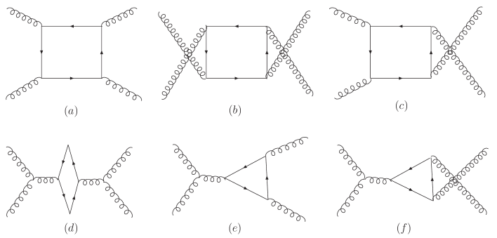
Figure 3: The diagrams contributing to quark pair production in TMD factorization approach. The gauge link structure of gluon TMD distributions associated with each diagram are different. The mirror diagrams are not shown.

As an effective TMD factorization is established in the quark pair production process, the measurement of the azimuthal asymmetries in pA collisions allows to probe directly the distribution of the linearly polarized gluons inside a large nucleus. Such measurements provide us with a first chance to explore the gluon polarization effect in the saturation regime. Since the magnitude of various linearly polarized gluon distributions are of the same magnitude as the unpolarized ones at small $x$ ( this becomes evident in the dilute limit where polarized and unpolarized distributions become identical), we also anticipate that these asymmetries are quite sizeable, suggesting a promising prospect for the extraction of polarized gluon distributions from quark pair production process. By comparing the gluon distributions extracted from this process with that probed in the other processes, like di-jet production in eA collisions, one could deduce how the gluon transverse momentum spectrum is affected by the different initial/final state interactions.

To emphasize the phenomenological relevance of our results, let us add that recently a strong back-to-back de-correlation of the two hadrons in $dAu$ collisions in the forward rapidity region of the deuteron was discovered by STAR and PHENIX [53, 54]. However, at RHIC energy, the dominant channel is $qg\rightarrow qg$ in the forward region. The $gg\rightarrow q\bar{q}$ channel only becomes relevant in the central rapidity region at RHIC. Apart from this, the effects caused by the polarized gluon distributions can not be isolated by only looking at the angular deviation from the back-to-back situation, but depend on the jet transverse energy [32]. Finally, it is important to mention that the small $x$ evolution effect has to be taken into account at LHC since the MV model is only a good model for high energy scattering when $x$ is not smaller than $0.01$ for a large nucleus. It should be feasible to measure these polarization dependent observables at RHIC and LHC. We plan to perform a complete set of phenomenological studies to investigate this possibility in the future.

5 Summary

In this paper, we have studied quark pair production in high energy proton-nucleus collisions in the central rapidity region and in the correlation limit where the total transverse momentum of the quark pair ($q_{\perp}$) is much smaller than the transverse momenta of the individual quarks ($\approx P_{\perp}$). Our main focus lay on the polarized case. We first used a hybrid approach to reproduce the full CGC result for quark pair production beyond the correlation limit. Our hybrid approach allowed us to take into account finite gluon transverse momentum effects on the proton side in a certain approximation. Employing a power expansion in the correlation limit, the multiple-point functions appearing in the full CGC result collapse into two-point functions and are thus given by a combination of gluon TMDs. All finite $N_{c}$ terms are kept in our calculation. The resulting cross section contains $\cos 2\phi$ and $\cos 4\phi$ dependent terms, where $\phi$ is the azimuthal angle between the transverse momenta $q_{\perp}$ and $P_{\perp}$. In addition to WW and dipole type linearly polarized gluon distributions, the novel linearly polarized gluon distribution $h^{\perp g}_{1,q\bar{q}}$ also generates $\cos 2\phi$ and $\cos 4\phi$ modulations. Such asymmetries could be measured at RHIC and LHC.

We further discussed our results in the dilute limit, the forward limit and the large $N_{c}$ limit, and found consistency with existing results in the different limits. The physical implications of the observed consistences were also addressed. In the end, we showed that a calculation based on TMD factorization leads to the same result as that obtained in the hybrid approach. The technique introduced in this paper can be extended to study di-jet production in other channels for pA collisions (e.g. di-jets initiated by different partons and/or various polarization channels). For these the linearly polarized gluon TMDs with different gauge link structures may also manifest themselves through $\cos 2\phi$ or $\cos 4\phi$ azimuthal dependencies of the cross sections. We would expect that exploring these polarization obervables at small $x$ will open a new path to investigate spin physics as well as saturation physics.

Acknowledgments: One of us (Jian Zhou) thanks Andreas Metz for suggesting this work to him and for helpful discussions. This work has been supported by BMBF (OR 06RY9191).

References

• [1] J. C. Collins and D. E. Soper, Nucl. Phys. B 193, 381 (1981) [Erratum-ibid. B 213, 545 (1983)] [Nucl. Phys. B 213, 545 (1983)]; Nucl. Phys. B 194, 445 (1982). J. C. Collins, D. E. Soper and G. F. Sterman, Nucl. Phys. B 250, 199 (1985).
• [2] X. -d. Ji, J. -p. Ma and F. Yuan, Phys. Rev. D 71, 034005 (2005) [hep-ph/0404183].
• [3] J. C. Collins and T. C. Rogers, arXiv:1210.2100 [hep-ph]. M. G. Echevarria, A. Idilbi and I. Scimemi, arXiv:1211.1947 [hep-ph]. T. Becher, M. Neubert and D. Wilhelm, JHEP 1202, 124 (2012) [arXiv:1109.6027 [hep-ph]]. and references therein
• [4] J. Collins, arXiv:1212.5974 [hep-ph].
• [5] G. Aad et al. [ATLAS Collaboration], arXiv:1212.5198 [hep-ex].
• [6] D. Boer, M. Diehl, R. Milner, R. Venugopalan, W. Vogelsang, D. Kaplan, H. Montgomery and S. Vigdor et al., arXiv:1108.1713 [nucl-th].
• [7] M. Anselmino et al., Eur. Phys. J.  A 47, 35 (2011) [arXiv:1101.4199 [hep-ex]].
• [8] J. Collins and J. -W. Qiu, Phys. Rev. D 75, 114014 (2007) [arXiv:0705.2141 [hep-ph]].
• [9] T. C. Rogers and P. J. Mulders, Phys. Rev. D 81, 094006 (2010) [arXiv:1001.2977 [hep-ph]].
• [10] F. Dominguez, B. W. Xiao and F. Yuan, Phys. Rev. Lett.  106, 022301 (2011) [arXiv:1009.2141 [hep-ph]].
• [11] F. Dominguez, C. Marquet, B. W. Xiao and F. Yuan, Phys. Rev.  D 83, 105005 (2011) [arXiv:1101.0715 [hep-ph]].
• [12] E. Avsar, arXiv:1203.1916 [hep-ph].
• [13] P. Nason, S. Dawson and R. K. Ellis, Nucl. Phys. B 303, 607 (1988); Nucl. Phys. B 327, 49 (1989) [Erratum-ibid. B 335, 260 (1990)].
• [14] S. Frixione, M. L. Mangano, P. Nason and G. Ridolfi, Adv. Ser. Direct. High Energy Phys.  15, 609 (1998) [hep-ph/9702287].
• [15] S. Catani, M. Ciafaloni, F. Hautmann, Nucl. Phys.  B366, 135-188 (1991).
• [16] J. C. Collins, R. K. Ellis, Nucl. Phys.  B360, 3-30 (1991).
• [17] E. M. Levin, M. G. Ryskin, Y. .M. Shabelski and A. G. Shuvaev, Sov. J. Nucl. Phys.  53, 657 (1991) [Yad. Fiz.  53, 1059 (1991)].
• [18] F. Gelis and R. Venugopalan, Phys. Rev. D 69, 014019 (2004) [hep-ph/0310090].
• [19] J. P. Blaizot, F. Gelis, R. Venugopalan, Nucl. Phys.  A743, 57-91 (2004). [hep-ph/0402257].
• [20] A. Schafer and J. Zhou, Phys. Rev. D 85, 114004 (2012) [arXiv:1203.1534 [hep-ph]].
• [21] L. D. McLerran and R. Venugopalan, Phys. Rev.  D 49, 2233 (1994) [arXiv:hep-ph/9309289]; Phys. Rev.  D 49, 3352 (1994) [arXiv:hep-ph/9311205].
• [22] A. H. Mueller, arXiv:hep-ph/0111244.
• [23] E. A. Kuraev, L. N. Lipatov, V. S. Fadin, Sov. Phys. JETP 45, 199-204 (1977).
• [24] L. V. Gribov, E. M. Levin, M. G. Ryskin, Phys. Rept.  100, 1-150 (1983).
• [25] P. J. Mulders and J. Rodrigues, Phys. Rev.  D 63, 094021 (2001) [arXiv:hep-ph/0009343].
• [26] M. Anselmino, M. Boglione, U. D’Alesio, E. Leader, S. Melis and F. Murgia, Phys. Rev. D 73, 014020 (2006) [hep-ph/0509035].
• [27] S. Meissner, A. Metz and K. Goeke, Phys. Rev.  D 76, 034002 (2007) [arXiv:hep-ph/0703176].
• [28] D. Boer and P. J. Mulders, Phys. Rev.  D 57, 5780 (1998) [arXiv:hep-ph/9711485].
• [29] S. J. Brodsky, D. S. Hwang and I. Schmidt, Phys. Lett.  B 530, 99 (2002) [arXiv:hep-ph/0201296].
• [30] J. C. Collins, Phys. Lett.  B 536, 43 (2002) [arXiv:hep-ph/0204004].
• [31] A. Metz, J. Zhou, Phys. Rev.  D84, 051503 (2011). [arXiv:1105.1991 [hep-ph]].
• [32] D. Boer, P. J. Mulders and C. Pisano, Phys. Rev.  D 80, 094017 (2009) [arXiv:0909.4652 [hep-ph]].
• [33] D. Boer, S. J. Brodsky, P. J. Mulders and C. Pisano, Phys. Rev. Lett.  106, 132001 (2011) [arXiv:1011.4225 [hep-ph]].
• [34] J. -W. Qiu, M. Schlegel and W. Vogelsang, Phys. Rev. Lett.  107, 062001 (2011) [arXiv:1103.3861 [hep-ph]].
• [35] D. Boer, W. J. den Dunnen, C. Pisano, M. Schlegel and W. Vogelsang, Phys. Rev. Lett.  108, 032002 (2012) [arXiv:1109.1444 [hep-ph]].
• [36] P. Sun, B. -W. Xiao, F. Yuan, Phys. Rev.  D84, 094005 (2011). [arXiv:1109.1354 [hep-ph]].
• [37] T. Liou, arXiv:1206.6123 [hep-ph].
• [38] D. Boer and C. Pisano, arXiv:1208.3642 [hep-ph].
• [39] S. Catani, M. Grazzini, Nucl. Phys.  B845, 297-323 (2011). [arXiv:1011.3918 [hep-ph]].
• [40] S. Mantry, F. Petriello, Phys. Rev.  D81, 093007 (2010). [arXiv:0911.4135 [hep-ph]]; and references therein.
• [41] P. M. Nadolsky, C. Balazs, E. L. Berger, C. -P. Yuan, Phys. Rev.  D76, 013008 (2007). [hep-ph/0702003 [HEP-PH]].
• [42] M. Garcia-Echevarria, A. Idilbi and I. Scimemi, arXiv:1111.4996 [hep-ph]. M. G. Echevarria, A. Idilbi, A. Schäfer and I. Scimemi, arXiv:1208.1281 [hep-ph].
• [43] I. Balitsky, Nucl. Phys.  B463, 99-160 (1996). [hep-ph/9509348].
• [44] L. D. McLerran, R. Venugopalan, Phys. Rev.  D59, 094002 (1999). [hep-ph/9809427].
• [45] E. Iancu, A. Leonidov and L. McLerran, arXiv:hep-ph/0202270.
• [46] Y. V. Kovchegov, Phys. Rev.  D 54, 5463 (1996) [arXiv:hep-ph/9605446].
• [47] J. Jalilian-Marian, A. Kovner, L. D. McLerran and H. Weigert, Phys. Rev.  D 55, 5414 (1997) [arXiv:hep-ph/9606337].
• [48] Y. V. Kovchegov, A. H. Mueller, Nucl. Phys.  B529, 451-479 (1998). [hep-ph/9802440]. B. Z. Kopeliovich, A. V. Tarasov, A. Schäfer, Phys. Rev.  C59, 1609-1619 (1999). [hep-ph/9808378]. A. Dumitru, L. D. McLerran, Nucl. Phys.  A700, 492-508 (2002). [hep-ph/0105268]. J. P. Blaizot, F. Gelis, R. Venugopalan, Nucl. Phys.  A743, 13-56 (2004). [hep-ph/0402256].
• [49] J. Jalilian-Marian, A. Kovner, A. Leonidov, H. Weigert, Phys. Rev.  D59, 014014 (1999). [hep-ph/9706377]. J. Jalilian-Marian, A. Kovner, A. Leonidov, H. Weigert, Nucl. Phys.  B504, 415-431 (1997). [hep-ph/9701284]. E. Iancu, A. Leonidov, L. D. McLerran, Nucl. Phys.  A692, 583-645 (2001). [hep-ph/0011241]. E. Ferreiro, E. Iancu, A. Leonidov, L. McLerran, Nucl. Phys.  A703, 489-538 (2002). [hep-ph/0109115].
• [50] A. Dumitru, J. Jalilian-Marian, Phys. Rev.  D81, 094015 (2010). [arXiv:1001.4820 [hep-ph]]; Phys. Rev.  D82, 074023 (2010) [arXiv:1008.0480 [hep-ph]]. F. Dominguez, A. H. Mueller, S. Munier, B. -W. Xiao, Phys. Lett.  B705, 106-111 (2011). [arXiv:1108.1752 [hep-ph]]. F. Dominguez, J. -W. Qiu, B. -W. Xiao and F. Yuan, Phys. Rev. D 85, 045003 (2012) [arXiv:1109.6293 [hep-ph]]. A. Dumitru, J. Jalilian-Marian, T. Lappi, B. Schenke and R. Venugopalan, Phys. Lett. B 706, 219 (2011) [arXiv:1108.4764 [hep-ph]]. E. Iancu and D. N. Triantafyllopoulos, JHEP 1111, 105 (2011) [arXiv:1109.0302 [hep-ph]]. JHEP 1204, 025 (2012) [arXiv:1112.1104 [hep-ph]].
• [51] Z. -t. Liang, X. -N. Wang and J. Zhou, Phys. Rev. D 77, 125010 (2008) [arXiv:0801.0434 [hep-ph]].
• [52] C. J. Bomhof, P. J. Mulders and F. Pijlman, Phys. Lett. B 596, 277 (2004) [hep-ph/0406099]; Eur. Phys. J. C 47, 147 (2006) [hep-ph/0601171].
• [53] E. Braidot [STAR Collaboration], Nucl. Phys. A 854, 168 (2011) [arXiv:1008.3989 [nucl-ex]].
• [54] A. Adare et al. [PHENIX Collaboration], Phys. Rev. Lett.  107, 172301 (2011) [arXiv:1105.5112 [nucl-ex]].