Evaluation of small elements of the eigenvectors of certain symmetric tridiagonal matrices with high relative accuracy

Abstract

Evaluation of the eigenvectors of symmetric tridiagonal matrices is one of the most basic tasks in numerical linear algebra. It is a widely known fact that, in the case of well separated eigenvalues, the eigenvectors can be evaluated with high relative accuracy. Nevertheless, in general, each coordinate of the eigenvector is evaluated with only high absolute accuracy. In particular, those coordinates whose magnitude is below the machine precision are not expected to be evaluated with any accuracy whatsoever.

It turns out that, under certain conditions, frequently ecountered in applications, small (e.g. $10^{-50}$) coordinates of eigenvectors of symmetric tridiagonal matrices can be evaluated with high relative accuracy. In this paper, we investigate such conditions, carry out the analysis, and describe the resulting numerical schemes. While our schemes can be viewed as a modification of already existing (and well known) numerical algorithms, the related error analysis appears to be new. Our results are illustrated via several numerical examples.

Keywords: symmetric tridiagonal matrices, eigenvectors, small elements, high accuracy, recurrence relations

Math subject classification: 65G99, 65F15, 65Q30

1 Introduction

The evaluation of eigenvectors of symmetric tridiagonal matrices is one of the most basic tasks in numerical linear algebra (see, for example, such classical texts as [3], [4], [5], [6], [8], [9], [19], [21], [22]). Several algorithms to perform this task have been developed; these include Power and Inverse Power methods, Jacobi Rotations, QR and QL algorithms, to mention just a few. Many of these algorithms have become standard and widely known tools.

In the case when the eigenvalues of the matrix in question are well separated, most of these algorithms will evaluate the corresponding eigenvectors to a high relative accuracy. More specifically, suppose that $n>0$ is an integer, that $A$ is an $n$ by $n$ symmetric matrix, that $\lambda$ is an eigenvalue of $A$, that $v\in\mathbb{R}^{n}$ is the corresponding unit-length eigenvector, and that $\hat{v}\in\mathbb{R}^{n}$ is its numerical approximation (produced by one of the standard algorithms). Then,

$$\|v-\hat{v}\|\leq M\cdot\varepsilon,$$ (1)

where $\|\cdot\|$ denotes the Euclidean norm, $\varepsilon$ is the machine precision (e.g. $\varepsilon\approx 10^{-16}$ for double precision calculations), and $M$ is proportional to the inverse of the distance between $\lambda$ and the rest of the spectrum of $A$.

However, a closer look at (1) reveals that it only guarantees that the coordinates of $v$ be evaluated to high absolute accuracy. This is due to the following trivial observation. Suppose that we add $\varepsilon$ to the first coordinate $\hat{v}_{1}$ of $\hat{v}$. Then, the perturbed $\hat{v}$ will not violate (1). On the other hand, the relative accuracy of $\hat{v}_{1}$ can be as large as

$$\frac{|v_{1}+\varepsilon-v_{1}|}{|v_{1}|}=\frac{\varepsilon}{|v_{1}|}.$$ (2)

In particular, if $|v_{1}|<\varepsilon$, then $\hat{v}_{1}$ is not guaranteed to approximate $v_{1}$ with any relative accuracy whatsoever.

Sometimes the poor relative accuracy of ”small” coordinates is of no concern; for example, this is usually the case when $v$ is only used to project other vectors onto it. Nevertheless, in several prominent problems, small coordinates of the eigenvector often need to be evaluated to high relative accuracy. Numerical evaluation of special functions provides a rich source of such problems; these include the evaluation of Bessel functions (see Sections 2.1, 2.2.2, 5.1), the evaluation of some quantities associated with prolate spheroidal wave functions (see Section 5.2, and also [18]), and the evaluation of singular values of the truncated Laplace transform (see [11]), among others.

In this paper, we describe a scheme for the evaluation of the coordinates of eigenvectors of certain symmetric tridiagonal matrices, to high relative accuracy. More specifically, we consider the matrices whose non-zero off-diagonal elements are constant (or approximately so), and whose diagonal elements constitute a monotonically increasing sequence (see, however, Remark 2 below). The connection of such matrices to Bessel functions and prolate spheroidal wave functions is discussed in Sections 2.2.2, 5.2, respectively. Also, we carry out detailed error analysis of our algorithm (see Sections 3.2, 3.3). While our scheme can be viewed as a modification of already existing (and well known) algorithms, such error analysis, perhaps surprisingly, appears to be new. In addition, we conduct several numerical experiments to illustrate the analysis, to demonstrate our scheme’s accuracy, and to compare the latter to that of some classical algorithms (see Section 6).

The following is one of the principal analytical results of this paper (see Theorem 19 in Section 3.3 for a more precise statement, and Theorems 13, 14, 15, Corollary 6 in Section 3.2 below for the treatment of a more general case).

Theorem 1.

Suppose that $a\geq 1$ is a real number, and that, for any real $c\geq 1$, $n=n(c)>c$ is an integer, the real numbers $A_{1}(c),\dots,A_{n}(c)$ are defined via the formula

$$A_{j}(c)=2+2\cdot\left(\frac{j}{c}\right)^{a},$$ (3)

for every $j=1,\dots,n$, and that the $n$ by $n$ symmetric tridiagonal matrix $A=A(c)$ is defined via the formula

$$A(c)=\begin{pmatrix}A_{1}&1&&&&\\ 1&A_{2}&1&&&\\ &1&A_{3}&1&&\\ &&\ddots&\ddots&\ddots&\\ &&&1&A_{n-1}&1\\ &&&&1&A_{n}\\ \end{pmatrix}.$$ (4)

Suppose furthermore that, for any real $c>1$, $\lambda(c)$ is an eigenvalue of $A(c)$, that $1<k(c)<n(c)$ is an integer, that

$$2+A_{k(c)}<\lambda(c)\leq 2+A_{k(c)+1}.$$ (5)

and that $X(c)=(X_{1},\dots,X_{n})\in\mathbb{R}^{n}$ is the unit-length $\lambda(c)-$eigenvector of $A(c)$. Suppose, in addition, that $\varepsilon>0$, and that the entries of $A(c)$ are defined to relative precision $\varepsilon$, for any $c>1$. Then, the first $k(c)$ coordinates $X_{1},\dots,X_{k}$ of $X(c)$ are defined to the relative precision $R(c,a)$, where

$$R(c,a)\leq\varepsilon\cdot O\left(-\log(X_{1})\right)\cdot O\left(c^{4\cdot a/(a+2)}\right),\quad c\to\infty.$$ (6)

Remark 1.

We observe that, according to (6), the relative precision of $X_{1},\dots,X_{k}$ depends only logarithmically on their order of magnitude. In other words, even if, say, $X_{1}$ is significantly smaller than $\varepsilon$, it is still defined to fairly high relative precision.

Remark 2.

The definition of the entries of the matrix $A$ in Theorem 1 is motivated by particular applications (see Section 5). On the other hand, Theorem 1 and Remark 1 generalize to a much wider class of matrices; these include, for example, perturbations of $A$, defined via (4); matrices whose diagonal entries are of a more general form than (3); banded (not necessarily tridiagonal) matrices, etc. While such generalizations are straightforward (and are based, in part, on the results of Section 3.1), the analysis is somewhat involved, and will be published at a later date (see, however, Theorems 13, 14 and Corollary 6 in Section 3.2 below for one such generalization).

The proof of Theorem 1 is constructive and somewhat technical (see Sections 3.2, 3.3). The resulting numerical algorithms for the evaluation of the eigenvector $X$ are described in Section 4.

In practice, the upper bound in (6) above seems to be overly pessimistic. In fact, the following conjecture has been verified by extensive numerical experiments (see Section 6).

Conjecture 1.

Suppose that, in addition to the hypothesis of Theorem 1 above, we evaluate the eigenvector $X(c)$ by the algorithm from Section 4.3. Then, for any real $c>1$ and any integer $1\leq j\leq k(c)$,

$$\text{\rm{rel}}(X_{j}(c))\leq 100\cdot c^{2\cdot a/(a+2)}\cdot\varepsilon.$$ (7)

In particular, $\text{\rm{rel}}(X_{1})$ does not depend on the magnitude of $X_{1}$, for any $c>1$.

We observe that the power of $c$ in (7) is half the power of $c$ in (6). In other words, Theorem 1 appears to overestimate the number of lost digits in the evaluation of the first $k$ elements of $X$ by roughly a factor of two.

The paper is organized as follows. In Section 2, we summarize a number of well known mathematical and numerical facts to be used in the rest of this paper. In Section 3, we develop the necessary analytical apparatus and perform error analysis of the algorithm, described in Section 4 (and we also describe a number of related algorithms). In Section 5, we discuss some applications of our algorithm to other computational problems. In Section 6, we illustrate the numerical stability of our algorithm and corresponding theoretical results via several numerical examples, and provide comparison to some related classical algorithms.

2 Mathematical and Numerical Preliminaries

In this section, we introduce notation and summarize several facts to be used in the rest of the paper.

2.1 Bessel Functions

In this section, we describe some well known properties of Bessel functions. All of these properties can be found, for example, in [1], [7].

Suppose that $n\geq 0$ is a non-negative integer. The Bessel function of the first kind $J_{n}:\mathbb{C}\to\mathbb{C}$ is defined via the formula

$$J_{n}(z)=\sum_{m=0}^{\infty}\frac{(-1)^{m}}{m!\cdot(m+n)!}\cdot\left(\frac{z}{2}\right)^{2m+n},$$ (8)

for all complex $z$. Also, the function $J_{-n}:\mathbb{C}\to\mathbb{C}$ is defined via the formula

$$J_{-n}(z)=(-1)^{n}\cdot J_{n}(z),$$ (9)

for all complex $z$.

The Bessel functions $J_{0},J_{\pm 1},J_{\pm 2},\dots$ satisfy the three-term recurrence relation

$$z\cdot J_{n-1}(z)+z\cdot J_{n+1}(z)=2n\cdot J_{n}(z),$$ (10)

for any complex $z$ and every integer $n$. In addition,

$$\sum_{n=-\infty}^{\infty}J^{2}_{n}(x)=1,$$ (11)

for all real $x$.

2.2 Numerical Tools

In this subsection, we summarize several numerical techniques to be used in this paper.

2.2.1 Shifted Inverse Power Method

Suppose that $n\geq 0$ is an integer, and that $A$ is an $n$ by $n$ real symmetric matrix. Suppose also that $\sigma_{1}<\sigma_{2}<\dots<\sigma_{n}$ are the eigenvalues of $A$. The Shifted Inverse Power Method iteratively finds the eigenvalue $\sigma_{k}$ and the corresponding eigenvector $v_{k}\in\mathbb{R}^{n}$, provided that an approximation $\lambda$ to $\sigma_{k}$ is given, and that

$$|\lambda-\sigma_{k}|<\max\left\{|\lambda-\sigma_{j}|\;:\;j\neq k\right\}.$$ (12)

Each Shifted Inverse Power iteration solves the linear system

$$\left(A-\lambda_{j}I\right)\cdot x=w_{j}$$ (13)

in the unknown $x\in\mathbb{R}^{n}$, where $\lambda_{j}$ and $w_{j}\in\mathbb{R}^{n}$ are the approximations to $\sigma_{k}$ and $v_{k}$, respectively, after $j$ iterations; the number $\lambda_{j}$ is usually referred to as ”shift”. The approximations $\lambda_{j+1}$ and $w_{j+1}\in\mathbb{R}^{n}$ (to $\sigma_{k}$ and $v_{k}$, respectively) are evaluated from $x$ via the formulae

$$w_{j+1}=\frac{x}{\|x\|},\quad\lambda_{j+1}=w_{j+1}^{T}\cdot A\cdot w_{j+1}$$ (14)

(see, for example, [3], [22] for more details).

Remark 3.

For symmetric matrices, the Shifted Inverse Power Method converges cubically in the vicinity of the solution. In particular, if the matrix $A$ is tridiagonal, and the initial approximation $\lambda$ is sufficiently close to $\sigma_{k}$, the Shifted Inverse Power Method evaluates $\sigma_{k}$ and $v_{k}$ essentially to machine precision $\varepsilon$ in $\displaystyle O\left(\log(-\log\varepsilon)\right)$ iterations, and each iteration requires $O(n)$ operations (see e.g [22], [3]).

2.2.2 Evaluation of Bessel Functions

Suppose that $x>0$ is a real number, and that $m>x$ is an integer. The classical scheme for the evaluation of $J_{0}(x),J_{1}(x),\dots,J_{m}(x)$ is based on (9), (10), (11) in Section 2.1 (see e.g [1], [13]) consists of the following steps.

• select integer $N>\max\left\{m,x\right\}$ (see Remark 4 below).

• set $X_{N}=1$ and $X_{N+1}=0$.

• evaluate $X_{N-1},X_{N-2},\dots,X_{1},X_{0}$ iteratively via the recurrence relation (10), in the direction of decreasing indices. In other words, for every $k=N,\dots,1$, evaluate $X_{k-1}$ via the formula

  $$X_{k-1}=\frac{2k}{x}\cdot X_{k}(x)-X_{k+1}(x),$$ (15)

• for every $k=0,\dots,m$, evaluate the approximation $\tilde{J}_{k}$ to $J_{k}(x)$ via

  $$\tilde{J}_{k}=X_{k}\cdot\left(X^{2}_{0}+2\cdot\sum_{l=1}^{N}X^{2}_{l}\right)^{-\frac{1}{2}}.$$ (16)

Remark 4.

In this paper, we always select sufficiently large $N$ so that the algorithm described above, when carried out in extended precision, evaluates $J_{0}(x),\dots,J_{m}(x)$ to at least 17 decimal digits. Further discussion of the matter is beyond the scope of this paper (see e.g. [1], [13] for more details).

3 Analytical Apparatus

The purpose of this section is to provide the analytical apparatus to be used in the rest of the paper.

3.1 Local Properties of Eigenvectors of Certain Tridiagonal Matrices

In this subsection, we develop several analytical results pertaining to the eigenvectors of certain tridiagonal symmetric matrices.

In the following theorem, we describe some obvious properties of the eigenvectors of certain tridiagonal symmetric matrices.

Theorem 2.

Suppose that $n>1$ is an integer, that $2<A_{1}<A_{2}<\dots$ is an increasing sequence of positive real numbers, and that the symmetric tridiagonal $n$ by $n$ matrix $A$ is defined via the formula

$$A=\begin{pmatrix}A_{1}&1&&&&\\ 1&A_{2}&1&&&\\ &1&A_{3}&1&&\\ &&\ddots&\ddots&\ddots&\\ &&&1&A_{n-1}&1\\ &&&&1&A_{n}\\ \end{pmatrix}.$$ (17)

Suppose also that the real number $\lambda$ is an eigenvalue of $A$, and that $x=(x_{1},\dots,x_{n})\in\mathbb{R}^{n}$ is an eigenvector corresponding to $\lambda$. Then,

$$x_{2} \;=\left(\lambda-A_{1}\right)\cdot x_{1}.$$ (18)

Also,

$$x_{j+1}=\left(\lambda-A_{j}\right)\cdot x_{j}-x_{j-1},$$ (19)

for every $j=2,\dots,n-1$. Finally,

$$x_{n-1} \;=\left(\lambda-A_{n}\right)\cdot x_{n}.$$ (20)

In particular, both $x_{1}$ and $x_{n}$ differ from zero, and $\lambda$ is simple.

Proof.

The identities (18), (19), (20) follow immediately from (17) and the fact that

$$A\cdot x=\lambda\cdot x.$$ (21)

We observe that the coordinates $x_{2},\dots,x_{n}$ are completely determined by $x_{1}$ and $\lambda$ via (18), (19), and hence the eigenvalue $\lambda$ is simple. Obviously, neither $x_{1}$ nor $x_{n}$ can be equal to zero, for otherwise $x$ would be the zero vector. ∎

In the following theorem, we assert that, under certain conditions, the first element of the eigenvectors of the matrix $A$ from Theorem 2 must be ”small”.

Theorem 3.

Suppose that the $n$ by $n$ symmetric tridiagonal matrix $A$ is defined via (17) in Section 3.1. Suppose also that $\lambda$ is an eigenvalue of $A$, and that $x=(x_{1},\dots,x_{n})\in\mathbb{R}^{n}$ is a corresponding eigenvector whose first coordinate is positive, i.e. $x_{1}>0$. Suppose, in addition, that $1\leq k\leq n$ is an integer, and that

$$\lambda\geq A_{k}+2.$$ (22)

Then,

$$0<x_{1}<x_{2}<\dots<x_{k}<x_{k+1}.$$ (23)

Also,

$$\frac{x_{j}}{x_{j-1}}>\frac{\lambda-A_{j}}{2}+\sqrt{\left(\frac{\lambda-A_{j}}{2}\right)^{2}-1},$$ (24)

for every $j=2,\dots,k$. In addition,

$$1<\frac{x_{k}}{x_{k-1}}<\dots<\frac{x_{3}}{x_{2}}<\frac{x_{2}}{x_{1}}.$$ (25)

Proof.

It follows from (22) that

$$\lambda_{k}-A_{1}>\lambda_{k}-A_{2}>\dots>\lambda_{k}-A_{k}\geq 2.$$ (26)

We combine (18), (19) in Theorem 2 with (26) to obtain (23) by induction. Suppose now that the real numbers $r_{1},\dots,r_{k}$ are defined via the formula

$$r_{j}=\frac{x_{j+1}}{x_{j}},$$ (27)

for every $j=1,\dots,k$, and that the real numbers $\sigma_{1},\dots,\sigma_{k}$ are defined via the formula

$$\sigma_{j}=\frac{\lambda-A_{j}}{2}+\sqrt{\left(\frac{\lambda-A_{j}}{2}\right)^{2}-1},$$ (28)

for every $j=1,\dots,k$. In other words, $\sigma_{j}$ is the largest root of the quadratic equation

$$x^{2}-\left(\lambda-A_{j}\right)\cdot x+1=0.$$ (29)

We observe that

$$\sigma_{1}>\dots>\sigma_{k}\geq 1,$$ (30)

due to (26) and (28). Also,

$$r_{1}>\sigma_{1}>\sigma_{2}>1,$$ (31)

due to the combination of (28) and (18). Suppose now, by induction, that

$$r_{j-1}>\sigma_{j}>1.$$ (32)

for some $2\leq j\leq k-1$. We observe that the roots of the quadratic equation (29) are $1/\sigma_{j}<1<\sigma_{j}$, and combine this observation with (32) to obtain

$$r_{j-1}^{2}-\left(\lambda-A_{j}\right)\cdot r_{j-1}+1>0.$$ (33)

We combine (33) with (27) and (19) to obtain

$$r_{j}=\frac{x_{j+1}}{x_{j}}=\frac{\left(\lambda-A_{j}\right)\cdot x_{j}-x_{j-1}}{x_{j}}=\lambda-A_{j}-\frac{1}{r_{j-1}}<r_{j-1}.$$ (34)

Also, we combine (28), (32), (34) to obtain

$$r_{j}=\lambda-A_{j}-\frac{1}{r_{j-1}}>\lambda-A_{j}-\frac{1}{\sigma_{j}}=\frac{\left(\lambda-A_{j}\right)\cdot\sigma_{j}-1}{\sigma_{j}}=\sigma_{j}>\sigma_{j+1}.$$ (35)

In other words, (32) implies (35), and we combine this observation with (31) to obtain

$$r_{1}>\sigma_{2},\quad r_{2}>\sigma_{3},\quad\dots,\quad r_{k-1}>\sigma_{k}.$$ (36)

Also, due to (34),

$$r_{1}>r_{2}>\dots>r_{k-1}.$$ (37)

We combine (27), (28), (36), (37) to obtain (24), (25). ∎

Corollary 1.

Under the assumptions of Theorem 3,

$$\frac{x_{k}}{x_{1}}>\prod_{j=2}^{k}\left(\frac{\lambda-A_{j}}{2}+\sqrt{\left(\frac{\lambda-A_{j}}{2}\right)^{2}-1}\right).$$ (38)

Remark 5.

In [17], the derivation of an upper bound on the first coordinate of an eigenvector of a certain matrix is based on a generalization of Theorem 3.

In the following theorem, we study the behavior of several last elements of an eigenvector of the matrix $A$ from Theorem 2 above.

Theorem 4.

Suppose that the $n$ by $n$ symmetric tridiagonal matrix $A$ is defined via (17) in Section 3.1. Suppose also that $\lambda$ is an eigenvalue of $A$, and that $x=(x_{1},\dots,x_{n})\in\mathbb{R}^{n}$ is a corresponding eigenvector whose last coordinate is positive, i.e. $x_{n}>0$. Suppose, in addition, that $1\leq k\leq n$ is an integer, and that

$$\lambda\leq A_{k}-2.$$ (39)

Then,

$$0<|x_{n}|<|x_{n-1}|<\dots<|x_{k}|<|x_{k-1}|.$$ (40)

Also,

$$-\frac{x_{j}}{x_{j+1}}>\frac{A_{j}-\lambda}{2}+\sqrt{\left(\frac{\lambda-A_{j}}{2}\right)^{2}-1},$$ (41)

for every $j=k,\dots,n-1$. In addition,

$$-1>\frac{x_{k}}{x_{k+1}}>\dots>\frac{x_{n-2}}{x_{n-1}}>\frac{x_{n-1}}{x_{n}}.$$ (42)

Proof.

The proof is essentially identical to that of Theorem 3 above and will be omitted. ∎

In the rest of this subsection, we investigate the behavior of the ”middle” elements of an eigenvector of the matrix $A$ from Theorems 2, 3, 4 above. We start with the following theorem.

Theorem 5.

Suppose that $k,m>0$ are integers, that $x_{k},\dots,x_{k+m+2}$ are real numbers, that $B_{k+1},\dots,B_{k+m+1}$ are real numbers, that

$$2>B_{k+1}>\dots>B_{k+m+1}\geq 0,$$ (43)

and that

$$x_{j+1}=B_{j}\cdot x_{j}-x_{j-1},$$ (44)

for every $j=k+1,\dots,k+m+1$. Suppose also that, for any real number $0<\theta\leq\pi/2$, the real $2\times 2$ matrix $A(\theta)$ is defined via the formula

$$A(\theta)=\begin{pmatrix}0&1\\ -1&2\cdot\cos(\theta)\end{pmatrix}.$$ (45)

Then,

$$\begin{pmatrix}x_{j+1}\\ x_{j+2}\end{pmatrix}=A\left(\arccos\left(\frac{B_{j+1}}{2}\right)\right)\cdot\begin{pmatrix}x_{j}\\ x_{j+1}\end{pmatrix},$$ (46)

for every $j=k,\dots,k+m$.

Proof.

The identity (46) follows from the combination of (44) and (45). ∎

Theorem 6.

Suppose that $k>0$ and $l>0$ are integers, and that

$$0<\theta_{k}<\theta_{k+1}<\dots<\theta_{k+l-1}\leq\frac{\pi}{4}\cdot\frac{1}{l+3/2}$$ (47)

are real numbers. Suppose also that $\varepsilon>0$, and that the sequence $x_{k},\dots,x_{k+l+2}$ is defined via the formulae

$$x_{k}=1,\quad x_{k+1}=1+\varepsilon,$$ (48)

and

$$\begin{pmatrix}x_{j+1}\\ x_{j+2}\end{pmatrix}=\begin{pmatrix}0&1\\ -1&2\cos(\theta_{j})\end{pmatrix}\begin{pmatrix}x_{j}\\ x_{j+1}\end{pmatrix},$$ (49)

for every $j=k,\dots,k+l-1$. Then,

$$x_{k},x_{k+1},\dots,x_{k+l},x_{k+l+1}>0.$$ (50)

In addition,

$$\frac{m+1}{m}>\frac{x_{k+m+1}}{x_{k+m}}>\frac{\cos\left((m+1/2)\cdot\theta_{k+l-1}\right)}{\cos\left((m-1/2)\cdot\theta_{k+l-1}\right)},$$ (51)

for every integer $m=1,2,\dots,l$; in particular,

$$1+\frac{1}{l}>\frac{x_{k+l+1}}{x_{k+l}}>1-\frac{1}{l+3/2}.$$ (52)

Proof.

We observe that

$$\frac{x_{k+m+1}}{x_{k+m}}=2\cdot\cos(\theta_{k+m-1})-\frac{x_{k+m-1}}{x_{k+m}},$$ (53)

for every $m=1,\dots,l$. We use (53) to prove (51) by induction on $m$. For $m=1$,

$$\frac{x_{k+2}}{x_{k+1}}=2\cdot\cos(\theta_{k})-\frac{1}{1+\varepsilon}<2,$$ (54)

and also

$$\frac{\cos(3\cdot\theta_{k+l-1}/2)}{\cos(\theta_{k+l-1}/2)} \;=4\cdot\cos(\theta_{k+l-1}/2)-3=2\cdot\cos(\theta_{k+l-1})-1$$

$$\;<2\cdot\cos(\theta_{k})-1<\frac{x_{k+2}}{x_{k+1}}.$$ (55)

By induction, for $2\leq m\leq l$,

$$\frac{x_{k+m+1}}{x_{k+m}}<2\cdot\cos(\theta_{k+m-1})-\frac{m-1}{m}<2-\frac{m-1}{m}=\frac{m+1}{m},$$ (56)

which proves the left-hand side of (51), and also

$$\frac{x_{k+m+1}}{x_{k+m}}>2\cdot\cos(\theta_{k+m-1})-\frac{\cos(\theta_{k+l-1}\cdot(m-3/2))}{\cos(\theta_{k+l-1}\cdot(m-1/2))}.$$ (57)

However, for any real $\theta$,

$$\frac{\cos(\theta\cdot(m-3/2))}{\cos(\theta\cdot(m-1/2))}+\frac{\cos(\theta\cdot(m+1/2))}{\cos(\theta\cdot(m-1/2))}=2\cdot\cos(\theta),$$ (58)

and we combine (57), (58) to conclude the right-hand side of (51). The inequality (51) implies (50). Next, we observe that

$$\cos(x)-\sin(x)\geq 1-\frac{4x}{\pi},$$ (59)

for all real $0\leq x\leq\pi/4$, and combine (59) with (47) to obtain

$$\frac{\cos\left((l+1/2)\cdot\theta_{k+l-1}\right)}{\cos\left((l-1/2)\cdot\theta_{k+l-1}\right)} \;=\cos\left(\theta_{k+l-1}\right)-\sin\left(\theta_{k+l-1}\right)\cdot\tan\left(\theta_{k+l-1}\cdot(l-1/2)\right)$$

$$\;>\cos\left(\theta_{k+l-1}\right)-\sin\left(\theta_{k+l-1}\right)$$

$$\;>1-\frac{4}{\pi}\cdot\frac{\pi}{4}\cdot\frac{1}{l+3/2}.$$ (60)

Finally, we combine (60) with (51) to obtain (52). ∎

Corollary 2.

If, in addition to (47),

$$\left(m+\frac{3}{2}\right)\cdot\theta_{k+m-1}<\frac{\pi}{4}$$ (61)

for every $m=1,\dots,l$, then

$$1+\frac{1}{m}>\frac{x_{k+m+1}}{x_{k+m}}>1-\frac{1}{m+3/2},$$ (62)

for every $m=1,\dots,l$.

Remark 6.

One can prove (along the lines of Theorem 6) that $x_{j+1}>x_{j}$ for every $j=k,\dots,k+l$, provided that $l<k$ and that $\varepsilon>k^{-1}$.

Theorem 7.

Suppose that $m>0$ is an integer, and $\theta_{1},\dots,\theta_{m}$ are real numbers such that

$$0<\theta_{1}<\dots<\theta_{m}\leq\frac{\pi}{2}.$$ (63)

Suppose also that, for any real number $0<\theta\leq\pi/2$, the real $2\times 2$ matrix $A(\theta)$ is defined via (45), and the complex $2\times 2$ matrices $D(\theta),\Lambda(\theta)$ are defined, respectively, via the formulae

$$D(\theta)=\begin{pmatrix}e^{i\theta}&0\\ 0&e^{-i\theta}\end{pmatrix},$$ (64)

$$\Lambda(\theta)=\begin{pmatrix}-2\cdot i\cdot\sin(\theta/2)&0\\ 0&2\cos(\theta/2)\end{pmatrix}.$$ (65)

Suppose furthermore that, for any real numbers $0<\eta_{1},\eta_{2}\leq\pi/2$, the complex $2\times 2$ matrix $D(\eta_{1},\eta_{2})$ is defined via the formula

$$D(\eta_{1},\eta_{2})=\begin{pmatrix}\sin(\eta_{1}/2)/\sin(\eta_{2}/2)&0\\ 0&\cos(\eta_{1}/2)/\cos(\eta_{2}/2)\end{pmatrix},$$ (66)

and that the unitary complex $2\times 2$ matrix $V$ is defined via the formula

$$V=\frac{1}{\sqrt{2}}\cdot\begin{pmatrix}-1&1\\ 1&1\end{pmatrix}.$$ (67)

Then,

$$A(\theta_{m})\cdot\dots\cdot A(\theta_{1})=$$

$$V\cdot\Lambda(\theta_{m})\cdot V\cdot$$

$$\quad D(\theta_{m})\cdot V\cdot D(\theta_{m-1},\theta_{m})\cdot V\cdot$$

$$\quad D(\theta_{m-1})\cdot V\cdot D(\theta_{m-2},\theta_{m-1})\cdot V\cdot$$

$$\quad\dots$$

$$\quad D(\theta_{2})\cdot V\cdot D(\theta_{1},\theta_{2})\cdot V\cdot$$

$$\quad D(\theta_{1})\cdot V\cdot\Lambda^{-1}(\theta_{1})\cdot V.$$ (68)

Proof.

Suppose that, for any real number $0<\theta\leq\pi/2$, the complex $2\times 2$ matrix $U(\theta)$ is defined via the formula

$$U(\theta)=\begin{pmatrix}1&e^{i\theta}\\ e^{i\theta}&1\\ \end{pmatrix}.$$ (69)

Obviously, $U(\theta)$ admits the decomposition

$$U(\theta)=e^{i\cdot\theta/2}\cdot V\cdot\Lambda(\theta)\cdot V.$$ (70)

Due to (70), the inverse of $U(\theta)$ admits the decomposition

$$U(\theta)^{-1}=e^{-i\cdot\theta/2}\cdot V\cdot\Lambda^{-1}(\theta)\cdot V.$$ (71)

Due to the combination of (70), (71),

$$U(\theta_{2})^{-1}\cdot U(\theta_{1}) \;=e^{i(\theta_{1}-\theta_{2})/2}\cdot V\cdot\Lambda^{-1}(\theta_{2})\cdot\Lambda(\theta_{1})\cdot V$$

$$\;=e^{i(\theta_{1}-\theta_{2})/2}\cdot V\cdot D(\theta_{1},\theta_{2})\cdot V.$$ (72)

We observe that, for any $0<\theta<\pi$,

$$\frac{i}{2\sin(\theta)}\cdot\begin{pmatrix}e^{-i\theta}&-1\\ -1&e^{-i\theta}\end{pmatrix}\begin{pmatrix}0&1\\ -1&2\cos(\theta)\end{pmatrix}\begin{pmatrix}1&e^{i\theta}\\ e^{i\theta}&1\end{pmatrix}=\begin{pmatrix}e^{i\theta}&0\\ 0&e^{-i\theta}\end{pmatrix},$$ (73)

and combine (73) with (70), (64), (45) to conclude that

$$A(\theta)=U(\theta)\cdot D(\theta)\cdot U^{-1}(\theta).$$ (74)

Subsequently, due to the combination of (70), (71), (72), (74),

$$A(\theta_{2})\cdot A(\theta_{1}) \;=U(\theta_{2})\cdot D(\theta_{2})\cdot U^{-1}(\theta_{2})\cdot U(\theta_{1})\cdot D(\theta_{1})\cdot U^{-1}(\theta_{1})$$

$$\;=V\cdot\Lambda(\theta_{2})\cdot V\cdot D(\theta_{2})\cdot V\cdot D(\theta_{1},\theta_{2})\cdot V\cdot D(\theta_{1})\cdot V\cdot\Lambda^{-1}(\theta_{1})\cdot V.$$ (75)

Now (68) follows from (75). ∎

Corollary 3.

Suppose that, for any complex square matrix $A$, we denote by $\sigma_{\min}(A)$ and $\sigma_{\max}(A)$, respectively, the minimal and maximal singular values of $A$. Then, under the assumptions of Theorem 7 above,

$$\sigma_{\min}(A(\theta_{m})\cdot\dots\cdot A(\theta_{1})\cdot V\cdot\Lambda(\theta_{1}))\geq 2\cdot\sin\left(\frac{\theta_{1}}{2}\right),$$ (76)

$$\sigma_{\max}(A(\theta_{m})\cdot\dots\cdot A(\theta_{1})\cdot V\cdot\Lambda(\theta_{1}))\leq 2\cdot\cos\left(\frac{\theta_{1}}{2}\right),$$ (77)

and also

$$\sigma_{\min}(A(\theta_{m})\cdot\dots\cdot A(\theta_{1}))\geq\tan\left(\frac{\theta_{1}}{2}\right),$$ (78)

$$\sigma_{\max}(A(\theta_{m})\cdot\dots\cdot A(\theta_{1}))\leq\cot\left(\frac{\theta_{1}}{2}\right).$$ (79)

Theorem 8.

Suppose, in addition to the hypothesis of Theorem 7, that $\delta>0$ is a real number, and that the vector $x\in\mathbb{R}^{2}$ is defined via the formula

$$x=\begin{pmatrix}1\\ 1+\delta\end{pmatrix}.$$ (80)

Then,

$$\frac{\min\left\{\left|A(\theta_{j})\cdot\dots\cdot A(\theta_{1})\cdot x\right|\;:\;1\leq j\leq m\right\}}{\max\left\{\left|A(\theta_{j})\cdot\dots\cdot A(\theta_{1})\cdot x\right|\;:\;1\leq j\leq m\right\}}\geq\frac{\theta_{1}}{2},$$ (81)

and also,

$$\frac{\left|A(\theta_{m})\cdot\dots\cdot A(\theta_{1})\cdot x\right|}{|x|} \;\leq 1+\frac{1}{2}\cdot\frac{(4/\theta_{1}^{2}-1)\cdot\delta^{2}}{(2+\delta)^{2}+\delta^{2}}.$$ (82)

Proof.

Due to the combination of (65), (67) and (80),

$$\Lambda^{-1}(\theta_{1})\cdot V\cdot x=\frac{1}{2\sqrt{2}}\cdot\begin{pmatrix}i\cdot\delta/\sin(\theta_{1}/2)\\ (2+\delta)/\cos(\theta_{1}/2)\end{pmatrix}.$$ (83)

We combine (83) with (68) and (77) to conclude that

$$\left|A(\theta_{m})\cdot\dots\cdot A(\theta_{1})\cdot x\right|\leq\frac{1}{\sqrt{2}}\left|\begin{pmatrix}\delta\cdot\cot(\theta_{1}/2)\\ 2+\delta\end{pmatrix}\right|\leq\frac{1}{\sqrt{2}}\left|\begin{pmatrix}2\cdot\delta/\theta_{1}\\ 2+\delta\end{pmatrix}\right|.$$ (84)

and

$$\left|A(\theta_{m})\cdot\dots\cdot A(\theta_{1})\cdot x\right|\geq\frac{1}{\sqrt{2}}\left|\begin{pmatrix}\delta\\ (2+\delta)\cdot\tan(\theta_{1}/2)\end{pmatrix}\right|\geq\frac{1}{\sqrt{2}}\left|\begin{pmatrix}\delta\\ (2+\delta)\cdot\theta_{1}/2\end{pmatrix}\right|.$$ (85)

It follows from (84) that

$$\left|A(\theta_{m})\cdot\dots\cdot A(\theta_{1})\cdot x\right|^{2}\leq\frac{1}{2}\cdot\left((2+\delta)^{2}+\left(\frac{2\cdot\delta}{\theta_{1}}\right)^{2}\right).$$ (86)

Also, it follows from (85) that

$$\left|A(\theta_{m})\cdot\dots\cdot A(\theta_{1})\cdot x\right|^{2}\geq\frac{1}{2}\cdot\left((2+\delta)^{2}+\left(\frac{2\cdot\delta}{\theta_{1}}\right)^{2}\right)\cdot\frac{\theta_{1}^{2}}{4}.$$ (87)

Now (81) follows from the combination of (86) and (87). Next we observe that, due to (80),

$$|x|^{2}=(1+\delta)^{2}+1=\frac{1}{2}\cdot\left((2+\delta)^{2}+\delta^{2}\right).$$ (88)

We combine (86) with (88) to conclude that

$$\frac{\left|A(\theta_{m})\cdot\dots\cdot A(\theta_{1})\cdot x\right|}{|x|}\leq\sqrt{1+\frac{(4/\theta_{1}^{2}-1)\cdot\delta^{2}}{(2+\delta)^{2}+\delta^{2}}},$$ (89)

which implies (82). ∎

Corollary 4.

Suppose, in addition to the hypotheses of Theorem 8, that $l\geq 1$ is an integer, that

$$\theta_{1}\cdot\left(l+\frac{5}{2}\right)\geq\frac{\pi}{4}$$ (90)

(compare to (47)), and that

$$-\frac{1}{l+3/2}<\delta<\frac{1}{l}$$ (91)

(see (52)). Then,

$$\frac{|x|}{9\cdot l}<\left|A(\theta_{m})\cdot\dots\cdot A(\theta_{1})\cdot x\right|<4\cdot|x|.$$ (92)

Proof.

The right inequality in (92) follows from the combination of (82), (90), (91). The left inequality in (92) follows from the combination of (90) and (81). ∎

3.2 Error Analysis

In Section 3.1 above, we investigated various analytical properties of eigenvectors of certain tridiagonal symmetric matrices. This section deals with stability issues pertaining to the numerical evaluation of such eigenvectors.

The following theorem is closely related to Theorem 3 in Section 3.1.

Theorem 9.

Suppose that $k>2$ is an integer, and that

$$B_{1}>B_{2}>\dots>B_{k}\geq 2$$ (93)

are real numbers. Suppose also that $x_{1},\dots,x_{k+1}$ are real numbers defined via the recurrence relation

$$x_{1}=1,$$

$$x_{2}=B_{1},$$

$$x_{j+1}=B_{j}\cdot x_{j}-x_{j-1},$$ (94)

for $j\geq 2$, and that the real numbers $r_{1},\dots,r_{k}$ are defined via the formula

$$r_{j}=\frac{x_{j+1}}{x_{j}},$$ (95)

for every $j=1,\dots,k$. Then,

$$r_{j}=B_{j}-\frac{1}{r_{j-1}},$$ (96)

for every $j=2,\dots,k$.

Proof.

The recurrence relation (96) follows from the combination of (94), (95). ∎

Theorem 10.

Suppose that $k>2$ is an integer, and that the real numbers $B_{1},\dots,B_{k}$, $x_{1},\dots,x_{k+1}$, $r_{1},\dots,r_{k}$ are those of Theorem 9 above. Suppose also that $\varepsilon>0$ is the machine precision, that $B_{1},\dots,B_{k}$ are defined to machine precision, and that $x_{1},\dots,x_{k+1}$, $r_{1},\dots,r_{k}$ are calculated, respectively, via (94), (96). Then,

$$\text{\rm{rel}}(r_{j})\leq(2\cdot j-1)\cdot\varepsilon,$$ (97)

for every $j=1,\dots,k$,

$$\text{\rm{rel}}(x_{j+1})\leq\varepsilon\cdot j^{2},$$ (98)

for every $j=1,\dots,k$, and also

$$\text{\rm{rel}}(x_{1}^{2}+x_{2}^{2}+\dots+x_{k}^{2}+x_{k+1}^{2})\leq\varepsilon\cdot 2\cdot k^{2}.$$ (99)

Proof.

First, suppose that $\varepsilon_{1},\dots,\varepsilon_{k}$ and $\delta_{1},\dots,\delta_{k}$ are real numbers, that

$$|\delta_{j-1}|\leq\varepsilon,$$ (100)

for every $j=2,\dots,k$, that

$$\hat{r}_{j-1}=r_{j-1}\cdot(1+\varepsilon_{j-1}),$$ (101)

for every $j=2,\dots,k$, that

$$\hat{B}_{j-1}=B_{j-1}\cdot(1+\delta_{j-1}),$$ (102)

for every $j=2,\dots,k$, and that

$$\hat{r}_{j}=\hat{B}_{j}-\frac{1}{\hat{r}_{j-1}},$$ (103)

for every $j=2,\dots,k$. Then, due to the combination of (101), (103), (96),

$$\hat{r}_{j} \;=\hat{B}_{j}-\frac{1}{r_{j-1}}+\frac{1}{r_{j-1}}-\frac{1}{\hat{r}_{j-1}}$$

$$\;=r_{j}\cdot\left(1+\frac{\varepsilon_{j-1}}{r_{j-1}\cdot r_{j}\cdot(1+\varepsilon_{j-1})}+\frac{B_{j}\cdot\delta_{j}}{r_{j}}\right).$$ (104)

Also, due to Theorem 3 in Section 3.1,

$$B_{1}=r_{1}>r_{2}>\dots>r_{k}>1,$$ (105)

and, moreover, for every $j=1,\dots,k$,

$$\frac{B_{j}}{r_{j}}<2.$$ (106)

We combine (100), (104), (105), (106) to conclude (97). Next, due to (95),

$$x_{j+1}=r_{1}\cdot r_{2}\cdot r_{3}\cdot\dots\cdot r_{j},$$ (107)

and we combine (107) with (97) to obtain

$$\text{\rm{rel}}(x_{j+1})\leq\varepsilon\cdot\left(1+3+\dots+2j-1\right),$$ (108)

for every $j=1,\dots,k-1$, which implies (98). Finally, due to (98),

$$\text{\rm{rel}}(x_{1}^{2}+\dots+x_{k+1}^{2}) \leq\frac{\sum_{j=1}^{k}x_{j+1}^{2}\cdot(1+\varepsilon\cdot j^{2})^{2}-(x_{1}^{2}+\dots+x_{k+1}^{2})}{x_{1}^{2}+\dots+x_{k+1}^{2}}$$

$$=\varepsilon\cdot\frac{\sum_{j=1}^{k}x_{j+1}^{2}\cdot(2\cdot j^{2}+\varepsilon\cdot j^{4})}{x_{1}^{2}+\dots+x_{k+1}^{2}},$$ (109)

which implies (99). ∎

Theorem 11.

Suppose that $k>0$ and $l>0$ are integers, that

$$0<\theta_{k}<\theta_{k+1}<\dots<\theta_{k+l-1}<\frac{\pi}{4}\cdot\frac{1}{l+3/2}$$ (110)

are real numbers, and that the real numbers $B_{k+1},\dots,B_{k+l}$ are defined via the formula

$$B_{j+1}=2\cdot\cos(\theta_{j}),$$ (111)

for every $j=k,\dots,k+l-1$. Suppose also that $\varepsilon>0$, that the real numbers $x_{k},x_{k+1}$ are those of Theorem 9 above, that the sequence $x_{k+2},\dots,x_{k+l+1}$ is defined via the formula

$$x_{j+2}=B_{j+1}\cdot x_{j+1}-x_{j},$$ (112)

for every $j=k,\dots,k+l-1$, and that the real numbers $r_{k},\dots,r_{k+l}$ are defined via (95) for every $j=k,\dots,k+l$. Suppose furthermore that $\varepsilon>0$ is the machine precision, that $B_{k+1},\dots,B_{k+l}$ are defined to precision $\varepsilon$, and that the precision of $r_{k},x_{k},x_{k+1}$ is described in (97), (98) of Theorem 10 above. Then,

$$\text{\rm{rel}}(x_{k+m+1})<\varepsilon\cdot(k+2\cdot m)^{2},$$ (113)

for every $m=1,\dots,l$. Also,

$$\text{\rm{rel}}(x_{k+2}^{2}+\dots+x_{k+l}^{2}+x_{k+l+1}^{2})<2\cdot\varepsilon\cdot(k+2\cdot l)^{2}.$$ (114)

In addition,

$$\text{\rm{rel}}(r_{k+l})<4\cdot(k+l)\cdot\varepsilon.$$ (115)

Proof.

Suppose that the real numbers $C_{1},\dots,C_{l}$ are defined via the formula

$$C_{j}=\frac{\cos\left((j-1/2)\cdot\theta_{k+l-1}\right)}{\cos\left((j+1/2)\cdot\theta_{k+l-1}\right)},$$ (116)

for every $j=1,\dots,l$. Then, due to (51),

$$\frac{1}{r_{k+j}}=\frac{x_{k+j}}{x_{k+j+1}}<C_{j},$$ (117)

for every $j=1,\dots,l$. It follows from (117) that

$$\frac{1}{r_{k+1}\cdot\dots\cdot r_{k+m-1}}<\frac{1}{\cos\left((m-1/2)\cdot\theta_{k+l-1}\right)},$$ (118)

for every $m=2,\dots,l$. Therefore,

$$\frac{1}{r_{k}\cdot r_{k+1}^{2}\cdot\dots\cdot r_{k+m-1}^{2}\cdot r_{k+m}} \;<\frac{C_{m}}{\cos^{2}\left((m-1/2)\cdot\theta_{k+l-1}\right)}$$

$$\;<\frac{1}{\cos^{2}\left((m+1/2)\cdot\theta_{k+l-1}\right)},$$ (119)

for every $m=2,\dots,l$. We observe that, similar to (96),

$$\frac{B_{k+m}}{r_{k+m}}=1+\frac{1}{r_{k+m}\cdot r_{k+m-1}},$$ (120)

for every $m=1,\dots,l$. Suppose that for every $j=k,k+1,\dots,k+l$ the relative errors of $r_{j},B_{j}$ are denoted, respectively, by $\varepsilon_{j},\delta_{j}$ (similar to (101), (102)). Due to the combination of (23), (96), (120),

$$\hat{r}_{k+m}=$$

$$r_{k+m}\cdot\left(1+\frac{\varepsilon_{k+m-1}}{r_{k+m-1}\cdot r_{k+m}\cdot(1+\varepsilon_{k+m-1})}+\;\delta_{k+m}\cdot\left(1+\frac{1}{r_{k+m-1}\cdot r_{k+m}}\right)\right),$$ (121)

for every $m=1,\dots,l$. In particular, using (117),

$$\varepsilon_{k+1}\leq\varepsilon_{k}\cdot C_{1}+\varepsilon\cdot(1+C_{1})\leq(\varepsilon_{k}+2\varepsilon)\cdot C_{1},$$ (122)

and, more generally,

$$\varepsilon_{k+m}<(\varepsilon_{k}+2\cdot m\cdot\varepsilon)\cdot C_{1}^{2}\cdot C_{2}^{2}\cdot\dots C_{k+m-1}^{2}\cdot C_{k+m},$$ (123)

for every $m=1,\dots,l$. Next, we combine (123) with (119) and Theorem 3 in Section 3.1 to conclude that

$$\varepsilon_{k+m}<(\varepsilon_{k}+2\cdot m\cdot\varepsilon)\cdot{\cos^{-2}\left((m+1/2)\cdot\theta_{k+l-1}\right)},$$ (124)

for every $m=1,\dots,l$. We substitute (110) into (124) to obtain the inequality

$$\varepsilon_{k+m}<(\varepsilon_{k}+2\cdot m\cdot\varepsilon)\cdot\cos^{-2}\left(\frac{\pi}{4}\cdot\frac{2m+1}{2l+3}\right)<2\cdot(\varepsilon_{k}+2\cdot m\cdot\varepsilon),$$ (125)

for every $m=1,\dots,l$. In particular, for $m=l$,

$$\varepsilon_{k+l}<2\cdot(\varepsilon_{k}+2\cdot l\cdot\varepsilon).$$ (126)

It follows from (125) that

$$\varepsilon_{k+1}+\cdots+\varepsilon_{k+m}<2\cdot m\cdot\varepsilon_{k}+2\cdot m\cdot(m+1)\cdot\varepsilon,$$ (127)

for every integer $m=1,\dots,l$. We observe that

$$x_{k+m+1}=x_{k+1}\cdot r_{k+1}\cdot\dots\cdot r_{k+m},$$ (128)

for every $m>1$, and hence (ignoring the $O(\varepsilon^{2})$ terms)

$$\text{\rm{rel}}(x_{k+m+1})<\text{\rm{rel}}(x_{k+1})+2\cdot m\cdot\varepsilon_{k}+2\cdot m\cdot(m+1)\cdot\varepsilon,$$ (129)

for every $m=1,2,\dots,l$. We combine (129) with Theorem 10 above to obtain (113), (114), and combine Theorem 10 with (126) to obtain (115). ∎

Theorem 12.

Suppose that $k>0$ and $0<l<m$ are integers, that $\theta_{k+l},\dots,\theta_{k+m}$ are real numbers such that

$$0<\frac{\pi}{2\cdot(2\cdot l+5)}\leq\theta_{k+l}<\dots<\theta_{k+m}\leq\frac{\pi}{2},$$ (130)

that $x_{k+l},\dots,x_{k+m+2}$ are real numbers, that $x_{k+l},x_{k+l+1}$ satisfy (52), and that $v_{k+l},\dots,v_{k+m+1}$ are vectors in $\mathbb{R}^{2}$ defined via the formula

$$v_{j}=\begin{pmatrix}x_{j}\\ x_{j+1}\end{pmatrix}$$ (131)

for every $j=k+l,\dots,k+m+1$. Suppose also that the real $2\times 2$ matrices $A(\theta_{k+l}),\dots,A(\theta_{k+m+1})$ are defined via (45), and that

$$v_{j+1}=A(\theta_{j})\cdot v_{j}$$ (132)

for every $j=k+l,\dots,k+m$. Suppose, in addition, that $\varepsilon>0$ is the machine precision, that $\cos(\theta_{k+j})$ are defined to relative precision $\varepsilon$ for every $j=l,\dots,m$, and that $v_{k+l+1},\dots,v_{k+m}$ are evaluated recursively via (132). Then,

$$\text{\rm{rel}}(v_{j})\leq 9\cdot l\cdot\text{\rm{rel}}(v_{k+l})\cdot\frac{\|v_{k+l}\|}{\|v_{j}\|},$$ (133)

for every $j=k+l+1,\dots,k+m+1$. Also,

$$\text{\rm{rel}}(v_{j})\leq 81\cdot l^{2}\cdot\text{\rm{rel}}(v_{k+l}),$$ (134)

for every $j=k+l+1,\dots,k+m+1$. Finally,

$$\text{\rm{rel}}\left(x_{k+l}^{2}+2\cdot\left(x_{k+l+1}^{2}+\dots+x_{k+m+1}^{2}\right)+x_{k+m+2}^{2}\right)\leq 162\cdot l^{2}\cdot\text{\rm{rel}}(v_{k+l}).$$ (135)

Proof.

Due to the combination of (130), (132) with (79) and (52),

$$\text{\rm{rel}}(v_{j})\cdot\|v_{j}\| \;\leq\cot\left(\frac{\theta_{k+l}}{2}\right)\cdot\|v_{k+l}\|\cdot\text{\rm{rel}}(v_{k+l})\leq\frac{2}{\theta_{k+l}}\cdot\|v_{k+l}\|\cdot\text{\rm{rel}}(v_{k+l})$$

$$\;\leq 9\cdot l\cdot\|v_{k+l}\|\cdot\text{\rm{rel}}(v_{k+l}),$$ (136)

for every $j=k+l+1,\dots,k+m+1$, which implies (133). The combination of (133) and (92) implies (134).

Thus, ignoring the $O(\varepsilon^{2})$ terms,

$$\text{\rm{rel}}(\|v_{j}\|^{2})=\text{\rm{rel}}(v_{j}\cdot v_{j})\leq 2\cdot\text{\rm{rel}}(v_{j})\leq 18\cdot l\cdot\text{\rm{rel}}(v_{k+l})\cdot\frac{\|v_{k+l}\|}{\|v_{j}\|},$$ (137)

for every $j=k+l+1,\dots,k+m+1$. Therefore,

$$\text{\rm{rel}}(\|v_{k+l}\|^{2}+\dots+\|v_{k+m+1}\|^{2})\leq$$

$$18\cdot l\cdot\text{\rm{rel}}(v_{k+l})\cdot\|v_{k+l}\|\cdot\frac{\|v_{k+l}\|+\dots+\|v_{k+m+1}\|}{\|v_{k+l}\|^{2}+\dots+\|v_{k+m+1}\|^{2}}.$$ (138)

We substitute (92) into (138) to obtain

$$\text{\rm{rel}}(\|v_{k+l}\|^{2}+\dots+\|v_{k+m+1}\|^{2})\leq 18\cdot 9\cdot l^{2}\cdot\text{\rm{rel}}(v_{k+l})\cdot\|v_{k+l}\|,$$ (139)

and substitute (131) into (139) to obtain (135). ∎

Corollary 5.

Suppose, in addition to the hypothesis of Theorem 12, that the relative accuracy of $x_{k+l}$ satisfies (113) in Theorem 11. Then,

$$\text{\rm{rel}}\left(x_{k+l}^{2}+\dots+x_{k+m+2}^{2}\right)\leq 162\cdot l^{2}\cdot(k+2\cdot l)^{2}\cdot\varepsilon.$$ (140)

Proof.

We observe that

$$\text{\rm{rel}}(x_{k+m+1}^{2}+2\cdot x_{k+m+2}^{2})\leq 2\cdot\text{\rm{rel}}\left((x_{k+m+1},x_{k+m+2})^{T}\right),$$ (141)

and combine this observation with (113), (135) to obtain (140). ∎

In the following two theorems, we summarize Theorems 9, 10, 11, 12 and Corollary 5 above.

Theorem 13.

Suppose that $k>0$, $l>0$ and $r>k+l$ are integers, that $B_{1},\dots,B_{r}$ is a sequence of real numbers, that

$$B_{1}>B_{2}>\dots>B_{k}\geq 2>B_{k+1}>\dots>B_{k+l}>2\cdot\cos\left(\frac{\pi}{4}\cdot\frac{1}{l+3/2}\right)$$ (142)

and that

$$2\cdot\cos\left(\frac{\pi}{4}\cdot\frac{1}{l+5/2}\right)\geq B_{k+l+1}>\dots>B_{r}\geq 0.$$ (143)

Suppose also that $\varepsilon>0$ is the machine precision, that $B_{1},\dots,B_{r}$ are defined to precision $\varepsilon$, and that the real numbers $x_{1},x_{2},\dots,x_{r+1}$ are evaluated from $B_{1},\dots,B_{r}$ via the recurrence relation (94). Then,

$$\text{\rm{rel}}(x_{j})\leq(j-1)^{2}\cdot\varepsilon,$$ (144)

for every $j=1,\dots,k+1$. Also,

$$\text{\rm{rel}}(x_{k+1+j})\leq(k+2\cdot j)^{2}\cdot\varepsilon,$$ (145)

for every $j=1,\dots,l$. In addition,

$$\text{\rm{rel}}\begin{pmatrix}x_{j-1}\\ x_{j}\end{pmatrix}\leq 81\cdot l^{2}\cdot(k+2\cdot l)^{2}\cdot\varepsilon,$$ (146)

$$\text{\rm{rel}}(x_{j})\leq 18\cdot l\cdot(k+2\cdot l)^{2}\cdot\left|\frac{x_{k+l}}{x_{j}}\right|\cdot\varepsilon$$ (147)

for every $j=k+l+1,\dots,r+1$. Finally,

$$\text{\rm{rel}}\left(x_{1}^{2}+\dots+x_{r}^{2}+x_{r+1}^{2}\right)\leq 162\cdot l^{2}\cdot(k+2\cdot l)^{2}\cdot\varepsilon.$$ (148)

Proof.

The combination of Theorems 10, 11, 12 and Corollary 5 above. ∎

Theorem 14.

Suppose that $n>0$ and $r,p,q>0$ are integers, that

$$r+p+q+1\leq n,$$ (149)

that $B_{r+1},\dots,B_{n}$ is a sequence of real numbers, that

$$B_{n}<\dots<B_{n+1-q}\leq-2<B_{n-q}<\dots<B_{n+1-p-q}<-2\cdot\cos\left(\frac{\pi}{4}\cdot\frac{1}{p+3/2}\right)$$ (150)

and that

$$-2\cdot\cos\left(\frac{\pi}{4}\cdot\frac{1}{p+5/2}\right)\leq B_{n-q-p}<\dots<B_{r+1}<0.$$ (151)

Suppose also that $\varepsilon>0$ is the machine precision, that $B_{r+1},\dots,B_{n}$ are defined to precision $\varepsilon$, and that the real numbers $y_{n},y_{n-1},\dots,y_{r+1},y_{r}$ are evaluated from $B_{r+1},\dots,B_{n}$ via the recurrence relation

$$y_{n}=1,$$

$$y_{n-1}=B_{n},$$

$$y_{j-1}=B_{j}\cdot y_{j}-y_{j+1},$$ (152)

for $j<n$ (similar to (94), but the direction is reversed). Then,

$$\text{\rm{rel}}(y_{n-j})\leq j^{2}\cdot\varepsilon,$$ (153)

for every $j=1,\dots,q$. Also,

$$\text{\rm{rel}}(y_{n-q-j})\leq(q+2\cdot j)^{2}\cdot\varepsilon,$$ (154)

for every $j=1,\dots,p$. In addition,

$$\text{\rm{rel}}\begin{pmatrix}y_{j+1}\\ y_{j}\end{pmatrix}\leq 81\cdot p^{2}\cdot(q+2\cdot p)^{2}\cdot\varepsilon,$$ (155)

$$\text{\rm{rel}}(y_{j})\leq 18\cdot l\cdot(k+2\cdot l)^{2}\cdot\left|\frac{y_{n-p-q}}{y_{j}}\right|\cdot\varepsilon,$$ (156)

for every $j=r,\dots,n-q-p-1$. Finally,

$$\text{\rm{rel}}\left(y_{n}^{2}+\dots+y_{r+2}^{2}\right)\leq 162\cdot p^{2}\cdot(q+2\cdot p)^{2}\cdot\varepsilon.$$ (157)

Proof.

We define $\tilde{B}_{1},\dots$ and $\tilde{x}_{1},\dots$ via the formula

$$\tilde{B}_{j}=-B_{n+1-j}$$ (158)

and

$$\tilde{x}_{j}=(-1)^{j+1}\cdot y_{n+1-j},$$ (159)

for $j\geq 1$. Then, due to the combination of (158), (159) with (152),

$$\tilde{x_{j+1}} \;=(-1)^{j}\cdot y_{n-j}$$

$$\;=(-1)^{j}\cdot\left(B_{n-(j-1)}\cdot y_{n-(j-1)}-y_{n-(j-2)}\right)$$

$$\;=(-1)^{(}j+1)\cdot\left(\tilde{B}_{j}\cdot\tilde{x}_{j}\cdot(-1)^{j+1}+\tilde{x}_{j-1}\cdot(-1)^{j}\right)$$

$$\;=\tilde{B}_{j}\cdot\tilde{x}_{j}-\tilde{x}_{j-1},$$ (160)

for $j\geq 2$. We conclude by combining (160) with (149), (150) and Theorem 13 above. ∎

Theorem 15.

Suppose, in addition to hypotheses of Theorems 13, 14, that the $n\times n$ matrix $B$, defined via the formula

$$B=\begin{pmatrix}B_{1}&1&&&&\\ 1&B_{2}&1&&&\\ &1&B_{3}&1&&\\ &&\ddots&\ddots&\ddots&\\ &&&1&B_{n-1}&1\\ &&&&1&B_{n}\\ \end{pmatrix},$$ (161)

is singular, that $x_{1},\dots,x_{r},x_{r+1}$ are those of Theorem 13, that $y_{r},y_{r+1},\dots,y_{n}$ are those of Theorem 14, that the real number $s$ is defined via the formula

$$s=\frac{x_{r}\cdot y_{r}+x_{r+1}\cdot y_{r+1}}{|x_{r}\cdot y_{r}+x_{r+1}\cdot y_{r+1}|}\cdot\sqrt{\frac{x_{r}^{2}+x_{r+1}^{2}}{y_{r}^{2}+y_{r+1}^{2}}},$$ (162)

and that the vector $z=(z_{1},\dots,z_{n})^{T}$ in $\mathbb{R}^{n}$ is defined via the formula

$$z=\left(x_{1},\dots,x_{r},x_{r+1},s\cdot y_{r+2},\dots,s\cdot y_{n}\right)^{T}.$$ (163)

Then, $z$ is an eigenvector of $B$ corresponding to the zero eigenvalue. Moreover,

$$\text{\rm{rel}}(s)\leq 81\cdot\left((q+2\cdot p)^{2}\cdot p^{2}+(k+2\cdot l)^{2}\cdot l^{2}\right)\cdot\varepsilon,$$ (164)

and

$$\text{\rm{rel}}(z_{1}^{2}+\dots+z_{n}^{2})\leq 243\cdot\left(p^{2}\cdot(q+2\cdot p)^{2}+(k+2\cdot l)^{2}\cdot l^{2}\right)\cdot\varepsilon.$$ (165)

Proof.

Due to Theorem 2 in Section 3.1, $x_{1},\dots,x_{r+1}$ are the first $r+1$ coordinates of an eigenvector of $B$ corresponding to the zero eigenvalue; also, $y_{r},\dots,y_{n}$ are the last $n+1-r$ coordinates of an eigenvector of $B$ in the same eigenspace. We combine this observation with Theorem 2 and (162) to conclude that $z$ is the eigenvector in the null-space of $B$ whose first coordinate is equal to $1$. The inequality (164) follows from the combination of (146) and (155) (in particular, $s$ in (162) is well defined). We combine (164) with (157) to obtain

$$\text{\rm{rel}}\left(s^{2}\cdot\left(y_{n}^{2}+\dots+y_{r+2}^{2}\right)\right)\leq$$

$$\left(3\cdot 81\cdot p^{2}\cdot(q+2\cdot p)^{2}+81\cdot(k+2\cdot l)^{2}\cdot l^{2}\right)\cdot\varepsilon.$$ (166)

Finally, we combine (166) with (148) to obtain (165). ∎

Corollary 6.

Suppose that, in addition to the hypothesis of Theorem 15, the vector $X\in\mathbb{R}^{n}$ is evaluated from $z$ in (163) via the formula

$$X=(X_{1},\dots,X_{n})^{T}=\frac{z}{\|z\|}.$$ (167)

Then,

$$\text{\rm{rel}}(X_{1})\leq 243\cdot\left(p^{2}\cdot(q+2\cdot p)^{2}+(k+2\cdot l)^{2}\cdot l^{2}\right)\cdot\varepsilon,$$ (168)

where $k,l,p,q,r$ are those of Theorems 13, 14. More generally,

$$\text{\rm{rel}}(X_{j})\leq\text{\rm{rel}}(X_{1})+\text{\rm{rel}}(x_{j}),$$ (169)

for every $2\leq j\leq r+1$, and

$$\text{\rm{rel}}(X_{j})\leq\text{\rm{rel}}(X_{1})+\text{\rm{rel}}(y_{j})+\text{\rm{rel}}(s),$$ (170)

for every $j=r+2,\dots,n$, where the sequences $\left\{x_{j}\right\}$, $\left\{y_{j}\right\}$ and the real number $s$ are those from Theorems 13, 14, 15.

3.3 Asymptotic Error Analysis of a Special Case

The analysis of Section 3.2 (e.g. Theorems 13, 14, 15 and Corollary 6) is carried out for a fairly general class of sequences $\left\{B_{j}\right\}$ (and related matrices $B$ defined via (161)). The resulting upper bounds on relative errors of coordinates of the null-space eigenvector of $B$ depend on the parameters $k,l,p,q$ determined from $\left\{B_{j}\right\}$ via (142), (143), (150), (151) (see e.g. the bounds in (165), (168)).

Despite the fact that these bounds are explicitly defined by $B$, the relation between the relative error of, say, the first coordinate $X_{1}$ of an eigenvector of unit norm and the magnitude of $X_{1}$ is not immediately obvious (see (168)). In this section, this relation is investigated in some detail for a special, but still fairly broad class of matrices $B$ (that also appear in various applications; see e.g. Section 5). First, we need a technical theorem.

Theorem 16.

Suppose that $a\geq 1$ is a real number, that $\delta>1$ is a real number, that the real number $D_{a}$ is defined via the formula

$$D_{a}=\sqrt{2}\cdot\int_{0}^{\pi/2}\left(\sin(\theta)\right)^{1+2/a}\;d\theta,$$ (171)

and that the real number $\alpha(a,\delta)$ is the solution of the equation

$$\alpha^{2}\cdot\left((1+\alpha)^{a}-1\right)\cdot\delta^{2}=\frac{\pi^{2}}{32}$$ (172)

in the unknown $\alpha$. Then,

$$\frac{2\cdot\sqrt{2}}{3}\leq D_{a}=\sqrt{\frac{\pi}{2}}\cdot\frac{\Gamma(1+1/a)}{\Gamma(3/2+1/a)},\leq\sqrt{2},$$ (173)

where $\Gamma$ is the standard Gamma function, and also

$$\alpha(a,\delta)\leq\left(\frac{\pi^{2}}{32\cdot a\cdot\delta^{2}}\right)^{1/3}.$$ (174)

Proof.

The proof is straightforward, elementary, and will be omitted. ∎

The rest of this section is dedicated to asymptotic error analysis pertaining to a certain class of symmetric tridiagonal matrices.

Theorem 17.

Suppose that $a\geq 1$ is a real number, that $\delta>1$ is a real number, that the real numbers $D_{a},\alpha(a,\delta)$ are those of Theorem 16 above. Suppose also that, for any real number $c\geq 1$, the real number $\kappa(c)$ is defined via the formula

$$\kappa(c)=\delta^{2/(a+2)}\cdot c^{a/(a+2)},$$ (175)

and the sequence $B_{1}(c),B_{2}(c),\dots$ is defined via the formula

$$B_{j}(c)=2+2\cdot\left(\frac{\kappa(c)}{c}\right)^{a}-2\cdot\left(\frac{j}{c}\right)^{a},$$ (176)

for every $j=1,2,\dots$. Suppose also that, for any real number $c\geq 1$, the sequence $x_{1}(c),x_{2}(c),\dots$ is defined from $\left\{B_{j}(c)\right\}$ via (94), and the integers $k=k(c),l=l(c)$ are defined from $\left\{B_{j}(c)\right\}$ via (142), (143). Then,

$$k=k(c)=\kappa(c)\cdot(1+o(c)),\quad c\to\infty,$$ (177)

$$l=l(c)=\alpha(a,\delta)\cdot\kappa(c)\cdot(1+o(c)),\quad c\to\infty,$$ (178)

and also

$$x_{1}(c)\leq x_{k}(c)\cdot\exp\left(-D_{a}\cdot\delta\cdot(1+o(1))\right),\quad c\to\infty.$$ (179)

Proof.

In this proof, we omit the dependence of various parameters on $c$ whenever it causes no confusion. First, (177) follows from the combination of (176), (175) and (142). We substitute (176), (177) into (38) to obtain

$$\frac{x_{k}}{x_{1}} \;\geq\prod_{j=2}^{k}\left(1+\left(\frac{\kappa}{c}\right)^{a}-\left(\frac{j}{c}\right)^{a}+\sqrt{\left(1+\left(\frac{\kappa}{c}\right)^{a}-\left(\frac{j}{c}\right)^{a}\right)^{2}-1}\right)$$

$$\;=\prod_{j=2}^{k}\left(1+\sqrt{2\cdot\left(\left(\frac{k}{c}\right)^{a}-\left(\frac{j}{c}\right)^{a}\right)}\right)\cdot(1+o(1)),\quad c\to\infty.$$ (180)

We define the real-valued function $g$ via the formula

$$g(x)=1+\sqrt{2\cdot\left(\left(\frac{k}{c}\right)^{a}-\left(\frac{x}{c}\right)^{a}\right)},$$ (181)

for real $0\leq x\leq k$, and combine (176), (175), (180), (181) to obtain

$$\prod_{j=2}^{k}\left(\frac{B_{j}}{2}+\sqrt{\left(\frac{B_{j}}{2}\right)^{2}-1}\right)=\exp\left((1+o(1))\cdot\int_{0}^{k}\log(g(x))\;dx\right),\quad c\to\infty.$$ (182)

Since $\log(g(k))=0$ due to (181),

$$\int_{0}^{k}\log(g(x))=-\int_{0}^{k}x\cdot\frac{d}{dx}\log(g(x))\;dx=-\int_{0}^{k}\frac{x\cdot g^{\prime}(x)}{g(x)}\;dx.$$ (183)

We combine (181) and (183) to obtain

$$\int_{0}^{k}\log(g(x))=\frac{a}{\sqrt{2}}\int_{0}^{k}\frac{x^{a}\;dx}{\sqrt{2}\cdot(k^{a}-x^{a})+\sqrt{c^{a}}\cdot\sqrt{k^{a}-x^{2}}}.$$ (184)

We perform the changes of variable

$$x^{a}=k^{a}\cdot\sin^{2}(\theta),$$ (185)

and substitute (185) into (184) to obtain

$$\int_{0}^{k}\log(g(x))=k\cdot\int_{0}^{\pi/2}\frac{\left(\sin(\theta)\right)^{1+2/a}\;d\theta}{\cos(\theta)+\sqrt{c^{a}/(2\cdot k^{a})}}.$$ (186)

Due to the combination of (186) and (171), (175), (177),

$$\int_{0}^{k}\log(g(x))=D_{a}\cdot\sqrt{\frac{k^{a+2}}{c^{a}}}\cdot(1+o(1)),\quad c\to\infty,$$ (187)

and we substitute (187) into (182) to obtain

$$\prod_{j=2}^{k}\left(\frac{B_{j}}{2}+\sqrt{\left(\frac{B_{j}}{2}\right)^{2}-1}\right)=\exp\left(D_{a}\cdot\sqrt{\frac{k^{a+2}}{c^{a}}}\cdot(1+o(1))\right),\quad c\to\infty.$$ (188)

We combine (188) with (175), (177) to obtain (179). Next, we combine (142), (143), (175), (176) to obtain

$$\frac{(k+l)^{a}-k^{a}}{c^{a}}=\frac{\pi^{2}}{32\cdot l^{2}}\cdot(1+o(1)),\quad c\to\infty.$$ (189)

If

$$k(c)\ll l(c),\quad c\to\infty,$$ (190)

then due to (189)

$$l^{a+2}=c^{a}\cdot\frac{\pi^{2}}{32}\cdot(1+o(1)),\quad c\to\infty,$$ (191)

in contradiction to the combination of (190) and (142), (143). If, on the other hand,

$$l\ll k,\quad c\to\infty,$$ (192)

then due to (189), (177)

$$l^{3}=\frac{c^{a}}{k^{a-1}}\cdot(1+o(c))=O\left(c^{a-(a-1)\cdot a/(a+2)}\right)=O\left(c^{3a/(a+2)}\right),\quad c\to\infty,$$ (193)

in contradiction to the combination of (192) and (142), (143). Therefore,

$$l(c)=O(k(c)),\quad c\to\infty,$$ (194)

and we combine (194) with (175), (177), (189) to obtain (178). ∎

The following theorem compliments Theorem 17 above.

Theorem 18.

Suppose that $a\geq 1$ and $\varepsilon>0$ are real numbers. Suppose also that, for any real number $c\geq 1$, the real numbers $\mu(c),\nu(c),\rho(c)$ are defined via the formulae

$$\mu(c)=\left(\frac{2^{1/a}\cdot c}{a}\right)^{1/3}\cdot\left(-\frac{3}{4}\cdot\log(\varepsilon)\right)^{2/3},$$ (195)

$$\nu(c)=2^{1/a}\cdot c+\mu(c),$$ (196)

$$\rho(c)=\left(\frac{\pi^{2}\cdot 2^{1/a}}{64\cdot a}\right)^{1/3}\cdot c^{1/3},$$ (197)

and that the integer $n(c)$ is defined via the formula

$$n(c)=\text{\rm{floor}}(\nu(c))+1.$$ (198)

Suppose furthermore that, for any real $c\geq 1$, the sequence $B_{1}(c),B_{2}(c),\dots,$ is defined via (176), that the integers $q=q(c)$ and $p=p(c)$ are defined from $\left\{B_{j}(c)\right\}$ via (150), (151), and that the sequence $y_{1}(c),\dots,y_{n}(c)$ is defined via (152). Then,

$$q(c)=\mu(c)\cdot(1+o(1)),\quad c\to\infty,$$ (199)

$$p(c)=\rho(c)\cdot(1+o(1)),\quad c\to\infty,$$ (200)

and also

$$|y_{n(c)}(c)|\leq\varepsilon\cdot|y_{n(c)+1-q(c)}(c)|\cdot(1+o(1)),\quad c\to\infty.$$ (201)

Proof.

We observe that, due to (175), (150),

$$2+2\cdot\left(\frac{\kappa(c)}{c}\right)^{a}-2\cdot\left(\frac{n(c)-q(c)}{c}\right)^{a}=-2+o(1),\quad c\to\infty,$$ (202)

and combine (202), (175), (177), (195), (196), (198) to obtain (199). We combine (197), (198), (199), (150), (151) to obtain

$$\frac{(n-q)^{a}-(n-q-p)^{a}}{c^{a}} \;=2\left(1-\left(1-\frac{p}{c\cdot 2^{1/a}}\right)^{a}\right)\cdot(1+o(1))$$

$$\;=\frac{\pi^{2}}{32\cdot p^{2}}\cdot(1+o(1)),\quad c\to\infty.$$ (203)

We combine (203) with (197) to obtain (200). Next, for $j=1,\dots,q(c)$,

$$B_{n-q+j} \;=-2\cdot\left(1+\left(\frac{n(c)-q(c)}{c}\right)^{a}\cdot\left(\left(1+\frac{j}{n(c)-q(c)}\right)^{a}-1\right)\right)$$

$$\;=-2\cdot\left(1+\frac{2\cdot a\cdot j}{2^{1/a}\cdot c}\right)\cdot(1+o(1)),\quad c\to\infty,$$ (204)

and hence, similar to (182),

$$\prod_{j=1}^{q}\left(\frac{B_{n-q+j}}{2}+\sqrt{\left(\frac{B_{n-q+j}}{2}\right)^{2}-1}\right)=$$

$$\exp\left((1+o(1))\cdot\int_{0}^{q}\log\left(1+\sqrt{\frac{4\cdot a\cdot x}{2^{1/a}\cdot c}}\right)\;dx\right),\quad c\to\infty.$$ (205)

We observe that

$$\int_{0}^{1}\log(1+Z\cdot\sqrt{s})\;ds=\frac{2\cdot Z}{3}\cdot(1+o(1)),\quad Z\to 0,$$ (206)

and combine (205), (205) and Theorem 4 in Section 3.1 to obtain

$$|y_{n}|\leq|y_{n-q+1}|\cdot\exp\left(-\frac{4}{3}\cdot\sqrt{\frac{a\cdot q^{3}}{2^{1/a}\cdot c}}\cdot(1+o(1))\right),\quad c\to\infty,$$ (207)

and combine (195), (199), (207) to obtain (201). ∎

The following theorem is a consequence of Theorems 17, 18 above.

Theorem 19.

Suppose that $\varepsilon>0$ is the machine precision, and that $a\geq 1$ and $1\leq\tilde{\delta}<\delta$ are real numbers. Suppose also that, for any real $c\geq 1$, we define $\mu(c)$ via (195), that $n(c)$ is an integer, that

$$2^{1/a}\cdot c<n(c)<2^{1/a}\cdot c+\mu(c)+1,$$ (208)

that the sequence $A_{1}(c),\dots,A_{n(c)}(c)$ is defined via the formula

$$A_{j}(c)=2+2\cdot\left(\frac{j}{c}\right)^{a},$$ (209)

for every $j=1,\dots,n(c)$, and the $n(c)\times n(c)$ matrix $A(c)$ is defined from $\left\{A_{j}(c)\right\}$ via (17). Suppose also that, for any $c\geq 1$, the real number $\lambda(c)$ is an eigenvalue of $A(c)$, that $\delta(c)$ is a real number, that

$$1<\tilde{\delta}<\delta(c)<\delta,$$ (210)

that

$$\lambda(c)=4+2\cdot\left(\frac{\delta(c)}{c}\right)^{2a/(a+2)},$$ (211)

and that $X(c)=(X_{1}(c),\dots,X_{n}(c))^{T}$ is the unit-norm $\lambda(c)$-eigenvector of $A(c)$. Suppose furthermore that, for any $c\geq 1$, the quantities $A_{j}(c)-\lambda(c)$ are defined to precision $\varepsilon$, for any $c\geq 1$ and every $j=1,\dots,n(c)$. Then,

$$|X_{1}(c)|<\exp\left(-\tilde{\delta}\cdot D_{a}\right)\cdot(1+o(1)),\quad c\to\infty,$$ (212)

where $D_{a}$ is defined via (171). Also, if $a>1$, then

$$\text{\rm{rel}}(X_{1}(c))\leq 620\cdot\delta^{(16-4a)/(3a+6)}\cdot c^{4a/(a+2)}\cdot\varepsilon\cdot(1+o(1)),\quad c\to\infty.$$ (213)

If $a=1$, then

$$\text{\rm{rel}}(X_{1}(c))\leq 960\cdot\left(\frac{\delta^{4/3}}{4}+\left(-\log\varepsilon\right)^{4/3}+1\right)\cdot c^{4/3}\cdot\varepsilon\cdot(1+o(1)),\quad c\to\infty.$$ (214)

Proof.

Suppose that $c\geq 1$, and that $k,l,p,q$ are defined from $A(c)$ via (142), (143), (150), (151), respectively. If $a>1$, we combine (208), (209), (210), (211) with Theorems 17, 18 above to obtain

$$243\cdot l^{2}\cdot(k+2\cdot l)^{2}=$$

$$243\cdot k^{4}\cdot\alpha^{2}\cdot(1+2\cdot\alpha)^{2}<$$

$$243\cdot\left(\frac{\pi^{2}}{32\cdot a}\right)^{2/3}\cdot\left(1+2\cdot\left(\frac{\pi^{2}}{32\cdot a}\right)\right)\cdot\delta^{8/(a+2)-4/3}\cdot c^{4a/(a+2)}<$$

$$620\cdot\delta^{(4/3)\cdot(4-a)/(a+2)}\cdot c^{4a/(a+2)}.$$ (215)

and combine (215) with Corollary 6 in Section 3.2 to obtain (213). If $a=1$, then we combine (208), (209), (210), (211) with Theorems 17, 18 above to obtain

$$243\cdot\left(l^{2}\cdot(k+2\cdot l)^{2}+p^{2}\cdot(q+2\cdot p)^{2}\right)\leq$$

$$243\cdot c^{4/3}\cdot\left(\frac{\pi^{2}}{32}\right)^{2/3}\cdot\left(\left(\delta^{2/3}+2\cdot\left(\frac{\pi^{2}}{32}\right)^{1/3}\right)^{2}+\left((-3\cdot\log\varepsilon)^{2/3}+2\cdot\left(\frac{\pi^{2}}{32}\right)^{1/3}\right)^{2}\right)$$

$$960\cdot c^{4/3}\cdot\left(\frac{\delta^{4/3}}{4}+\left(-\log\varepsilon\right)^{4/3}+1\right),$$ (216)

and combine (216) with Corollary 6 in Section 3.2 to obtain (214). For any $a\geq 1$, the inequality (212) follows now from (179). ∎

Remark 7.

The conclusions of Theorem 19 above hold even under a milder assumption that each of $A_{j}(c)$ and $\lambda(c)$ separately is defined to relative precision $\varepsilon$ for every $j$ (and not necessarily their difference). The related analysis (beyond the scope of this paper) is based on Theorems 13, 14 in Section 3.2, and on the observation that when $\lambda(c)\approx A_{j}(c)$ what matters is the absolute (and not relative) accuracy of $\lambda(c)-A_{j}(c)$.

4 Numerical Algorithms

In this section, we describe several numerical algorithms for the evaluation of the eigenvectors of certain symmetric tridiagonal matrices.

4.1 Problem Settings

Suppose that $n>0$ is an integer, that $2<A_{1}<A_{2}<\dots$ is a sequence of positive real numbers, that $A$ is an $n$ by $n$ symmetric tridiagonal matrix defined via (17) in Section 3.1, and that the real number $\lambda$ is an eigenvalue of $A$.

Task. Evaluate the unit-length eigenvector

$$X=(X_{1},\dots,X_{n})\in\mathbb{R}^{n}$$ (217)

of $A$ corresponding to $\lambda$.

Desired accuracy of the solution. We want the coordinates $X_{j}$ of $X$ to be evaluated to high relative accuracy (as opposed to absolute accuracy; see also Section 1).

Observation. This task is potentially difficult if $|X_{j}|$ is small compared to $\|X\|=1$. For example, if $|X_{1}|<\varepsilon$, where $\varepsilon$ is the machine precision (e.g. $\varepsilon\approx 10^{-16}$ for double-precision calculations), it is not obvious why $X_{1}$ should be evaluated to any correct digit at all (see also Section 1).

Observation. Due to Theorem 2 in Section 3.1,

$$X_{j-1}+\left(A_{j}-\lambda\right)\cdot X_{j}+X_{j+1}=0,$$ (218)

for every $j=2,\dots,n-1$. Qualitatively, the relation between $X_{j-1},X_{j},X_{j+1}$ depends on whether $\left(A_{j}-\lambda\right)$ is greater than 2, is less than -2, or is between -2 and 2 (see Section 3.1).

Assumption on $\lambda$. For the sake of clarity of presentation, in the rest of this section we assume that the eigenvalue $\lambda$ satisfies the inequality

$$2+A_{1}<\lambda<A_{n}-2.$$ (219)

Clearly, the obvious simplification of the algorithm described below will handle any eigenvalue $\lambda$ of $A$.

4.2 Informal Description of the Algorithm

This section contains an informal description of an algorithm for the evaluation of $X=(X_{1},\dots,X_{n})\in\mathbb{R}^{n}$ (see (217)). On the other hand, Section 4.3 below contains a complete outline of the steps of the algorithm.

Suppose that $1<r<n$ is an integer, and that

$$A_{r}\leq\lambda<A_{r+1}$$ (220)

(see (143), (151)). For any $\lambda-$eigenvector $x=(x_{1},\dots,x_{n})\in\mathbb{R}^{n}$ of $A$ and every $j=2,\dots,n-1$, the three consecutive coordinates $x_{j-1},x_{j},x_{j+1}$ satisfy the recurrence relation (19) of Theorem 2 (see also (218) above).

We set $x_{1}=1$ and use (19) to iteratively evaluate $x_{2},\dots,x_{r+1}$ (e.g. ”going forward”). Obviously, we have evaluated the first $r+1$ coordinates of $X$ up to a scaling constant. Next, we set $y_{n}=1$ and use (19) to iteratively evaluate $y_{n-1},y_{n-2},\dots,y_{r}$ (e.g. ”going backward”). Again, this gives the last $n-r+1$ coordinates of $X$ up to a different scaling constant. The accuracy of both evaluations is investigated in detail in Section 3.2.

The indices of the two sequences overlap at $j=r,r+1$. In exact arithmetic, the planar vectors $(x_{r},x_{r+1})$ and $(y_{r},y_{r+1})$ are linearly dependent (see Theorem 15 in Section 3.2). We ”glue the two sequences together” by multiplying $y_{r},\dots,y_{n}$ through by the correct scaling factor $s$; in particular, $x_{j}=s\cdot y_{j}$ for $j=r,r+1$. The resulting vector $z$ in $\mathbb{R}^{n}$ is a $\lambda-$eigenvector of $A$ (see Theorem 15). We then normalize it to obtain $X$.

4.3 Short Description of the Algorithm

Suppose that $n>0$ is an integer, that the $n$ by $n$ matrix $A$ is that from Section 4.1, that $\lambda$ is an eigenvalue of $A$, and that the integer $1<r<n$ is defined via (220) above.

Step A: evaluation of the left coordinates of $X$ (see (217)).

1. Set $x_{1}=1$.

2. Compute $x_{2}$ via (18) of Theorem 2.

3. Compute $x_{3},\dots,x_{r},x_{r+1}$ iteratively via (19) of Theorem 2.

Step B: evaluation of the right coordinates of $X$.

1. Set $y_{n}=1$.

2. Compute $y_{n-1}$ via (20) of Theorem 2.

3. Compute $y_{n-2},\dots,y_{r+1},y_{r}$ iteratively via (19) of Theorem 2.

Step C: glue them together.

1. Compute the real number $s$ via (162) in Theorem 15.

2. Compute the vector $z=(z_{1},\dots,z_{n})$ via (163) in Theorem 15.

3. Compute the vector $X=(X_{1},\dots,X_{n})$ from $z$ via (167) in Corollary 6.

Observation. The vector $X\in\mathbb{R}^{n}$ is the unit-norm $\lambda-$eigenvector of $A$ whose first coordinate is positive (see Corollary 6 in Section 3.2).

Running time. Obviously, the running time of this algorithm is $O(n)$ operations, where $n$ is the dimensionality of the matrix.

4.4 Accuracy

In Sections 4.2, 4.3, we described an algorithm for the evaluation of the unit length $\lambda-$eigenvector $X=(X_{1},\dots,X_{n})$ of $A$, whose first coordinate is positive. The accuracy of this procedure is investigated in some detail in Section 3.2 for a general tridiagonal matrix with constant off-diagonal elements and monotone diagonal. More specifically, the relative accuracy of various coordinates is described in Theorems 13, 14, 15 and Corollary 6 in Section 3.2. For example, (168) provides a bound on $\text{\rm{rel}}(X_{1})$ in terms of the integers $1<k,l,p,q<n$ (defined via (142), (143), (150), (151)) and the relative accuracy $\varepsilon$ of $\lambda-A_{j}$ for $j=1,\dots,n$ (see also Remark 7 in Section 3.3). We summarize the results of Section 3.2 qualitatively in the following observations (see also Section 6 for related numerical experiments).

Observation 1. For all $j$ such that $\lambda-A_{j}\geq 2$ (e.g. for $1\leq j\leq k$ in the notation of Theorem 13 in Section 3.2), the coordinates $X_{j}$ are evaluated to roughly the same relative accuracy, independent of how small they are (see e.g. Theorem 10 in Section 3.2 and (144) in Theorem 13). These coordinates form a monotonically increasing sequence (see Theorem 3 in Section 3.1 for an estimate on its growth).

Observation 2. For all $j$ such that $\lambda-A_{j}\leq-2$ (e.g. for $n-q\leq j\leq n$ in the notation of Theorem 14 in Section 3.2), the coordinates $X_{j}$ are evaluated to roughly the same relative accuracy, independent of how small they are (see e.g. (153) in Theorem 14). These coordinates form an alternating sequence, and their absolute values form a monotonically decreasing sequence (see Theorem 4 in Section 3.1 for an estimate on its decay).

Observation 3. For all $j$ such that $\lambda-2\leq A_{j}\leq\lambda+2$ (e.g. for $k<j<n-q$ in the notation of Theorems 13, 14) in Section 3.2, the coordinates $X_{j}$ are evaluated to roughly the same absolute accuracy (see e.g. (133) in Theorem 12, (146), (147) in Theorem 13, (155), (156) in Theorem 14). These coordinates vary in magnitude in a fairly moderate way and exhibit an oscillatory behavior (see e.g. Theorems 7, 8 and Corollaries 3, 4 in Section 3.1, and also Section 6).

Remark 8.

Extensive numerical experiments seem to indicate that the estimates from Section 3.2 are somewhat pessimistic. In other words, in practice the relative error tends to be smaller than our estimates suggest (see also Section 6).

Remark 9.

It is somewhat surprising that, according to (169) in Corollary 6, the relative error of, say, $X_{1}$ seems to be independent of the order of magnitude of $X_{1}$. In particular, while $X_{1}$ can be fairly small (see e.g. Theorem 3 and Corollary 1 in Section 3.1), it still will be evaluated to reasonable relative precision.

Remark 10.

When the coordinates of the eigenvector are evaluated via the three-terms recurrence (19), the choice of direction plays a crucial role. Roughly speaking, this recurrence is unstable in the backward direction in the region of growth, and is unstable in the forward direction in the region of decay (see also Section 3.2). As expected, the use of this recurrence relation in a ”wrong” direction leads to a disastrous loss of accuracy.

4.5 Related Algorithms

In Section 4.2, 4.3, we presented an algorithm for accurate evaluation of the coordinates of the eigenvector $X$ (see (217) in Section 4.1). In this section, we briefly discuss the accuracy of several classical algorithms for the solution of the same problem.

4.5.1 Inverse Power

The unit-length $\lambda-$eigenvector $X$ of $A$ can be obtained via Inverse Power Method with Shifts (see Section 2.2.1 for more details). This method is iterative, and, on each iteration, the approximation $x^{(k+1)}$ of $X$ is obtained from $x^{(k)}$ via solving the linear system

$$\left(\lambda\cdot I-A\right)\cdot x^{(k+1)}=x^{(k)},$$ (221)

and normalizing the solution. We observe that this method also evaluates $\lambda$ (even though in Section 4.1 we assume that $\lambda$ has already been evaluated). On each iteration, we solve the linear system (221) by Gaussian elimination (since $A$ is tridiagonal, each iteration costs $O(n)$ operations; moreover, $O(1)$ iterations are required: see Remark 3 in Section 2.2.1).

The following conjecture about the accuracy of Inverse Power Method is substantiated by extensive numerical experiments (see Section 6).

Conjecture 2.

Suppose that $\varepsilon>0$ is the machine precision (e.g. $\varepsilon\approx 10^{-16}$ for double-precision calculations), and that the eigenvalue $\lambda$ of $A$ is defined to accuracy $\varepsilon$. Suppose also that $\lambda-A_{1}>2$. Suppose furthermore that $K>0$ is an integer, and that

$$K>\frac{\log\left(|X_{1}|\right)}{\log(\varepsilon)}+1,$$ (222)

where $X=(X_{1},\dots,X_{n})\in\mathbb{R}^{n}$ is the unit-length $\lambda-$eigenvector of $A$. Then, after $K$ iterations of Inverse Power Method, $X_{1}$ is evaluated to high relative accuracy. More specifically, this relative accuracy is roughly of the same order of magnitude as for the algorithm described in Sections 4.2, 4.3 (see also (228), (233) below).

Remark 11.

The inequality (222) reflects on the fact that each iteration of Inverse Power Method can reduce the coordinates of the approximation $x^{(k)}$ by a factor of at most $\varepsilon^{-1}$. In other words, if $X_{1}\approx 10^{-50}$, and, in the initial approximation, $x^{(1)}_{1}=O(1)$, then $x^{(4)}_{1}$ will already be of the same order of magnitude as $X_{1}$, and $x^{(5)}$ will approximate $X_{1}$ to a high relative precision.

4.5.2 Jacobi Rotations

In the view of Section 4.5.1, one might suspect that virtually any standard algorithm would accurately solve the problem introduced in Section 4.1. In other words, one might suspect that the small coordinates of $X$ in the region of growth and the region of decay will be evaluated to high relative precision by any reasonable algorithm that computes eigenvectors.

Unfortunately, this is emphatically not the case, and the accuracy of the result strongly depends on the choice of the algorithm. For example, the popular Jacobi Rotations algorithm for the evaluation of the eigenvalues and eigenvectors of a symmetric matrix $A$ (see, for example, [3], [6], [21], [22]) typically evaluates the eigenvalues of $A$ fairly accurately. Moreover, the corresponding unit-length eigenvectors are evaluated to high relative accuracy, in the sense of (1) in Section 1. However, the coordinates of $X$ are typically evaluated only to high absolute accuracy. In particular, the relative accuracy of small coordinates will typically be poor: if, for example, $X_{1}\approx 10^{-50}$, its numerical approximation, produced by Jacobi Rotations, will usually have no correct digits at all (the latest statement is supported by extensive numerical evidence).

4.5.3 Gaussian Elimination

Another possible method to evaluate $X$ would be to solve the linear system

$$\left(\lambda\cdot I-A\right)\cdot X=0,$$ (223)

by means of Gaussian Elimination (see, for example, [3], [6], [21], [22]). Unfortunately, this method, in general, fails to evaluate the small coordinates of $X$ with high relative accuracy (see, however, Section 4.5.1, where Gaussian Elimination is used several times, as a step of Inverse Power Method).

5 Applications

In this section, we describe some applications of the algorithm from Section 4 to other computational problems.

5.1 Bessel Functions

Suppose that $x>0$ is a real number, and that $m>0$ is an integer. Below we describe a connection between the classical algorithm for the evaluation of $J_{0}(x),J_{\pm 1}(x),\dots,J_{\pm}(x)$ from Section 2.2.2 and the scheme from Section 4.3.

Suppose that $N>m$ is an integer (see Remark 4 in Section 2.2.2), that the symmetric tridiagonal $(2N+1)\times(2N+1)$ matrix $A=A(x)$ is that of Theorem 19 in Section 3.3 with $a=1$ and $c=x$ (see (209)), and that the real number $\lambda$ is defined via the formula

$$\lambda=2+\frac{2\cdot(N+1)}{x}.$$ (224)

In the notation of Section 2.2.2, $\lambda$ is an eigenvalue of $A$, and the corresponding unit-length eigenvector $X$ is precisely

$$X=\frac{1}{d}\cdot\left(\tilde{J}_{N},\dots,\tilde{J}_{1},\tilde{J}_{0},-\tilde{J}_{1},\dots,(-1)^{N}\cdot\tilde{J}_{N}\right).$$ (225)

In addition, the evaluation $\tilde{J}_{0},\dots,\tilde{J}_{N}$ via the scheme described in Section 2.2.2 (see (16)) is essentially identical to the evaluation of $X$ in (225) via the algorithm from Section 4.3.

We conclude that the accuracy of this evaluation has been analyzed in Theorems 17, 18 in Section 3.3, and, despite the scheme being classical, this analysis appears to be new (see (214) in Theorem 19 in Section 3.3 and Conjecture 1 in Section 1, as well as Section 6.3 for the related numerical experiments).

5.2 Prolate Spheroidal Wave Functions

Suppose that $c>0$ is a real number, and that the integral operator $F_{c}:L^{2}[-1,1]\to[-1,1]$ is defined via the formula

$$F_{c}[\varphi](x)=\int_{-1}^{1}\varphi(t)\cdot e^{icxt}\;dt.$$ (226)

Suppose also that the complex numbers $\lambda_{0}(c),\lambda_{1}(c),\dots$ are the eigenvalues of $F_{c}$ (ordered such that $|\lambda_{0}(c)|>|\lambda_{1}(c)|>\dots$). The prolate spheroidal wave functions (PSWFs) corresponding to the band limit $c$ are the unit-norm eigenfunctions $\psi_{0}^{(c)},\psi_{1}^{(c)},\dots$ of $F_{c}$ (see e.g. [23], [12], [20], [10], [15]).

It turns out that, for any $n\geq 0$, the eigenvalue $\lambda_{n}(c)$ can be evaluated at $O(1)$ operations from the first coordinate of the unit-length eigenvector corresponding to a certain eigenvalue of a symmetric tridiagonal matrix $A(c)$; moreover, this matrix is essentially a perturbed version of the matrix from Theorem 19 in Section 3.3, with $a=2$ (see e.g. [18], [15] for more details).

In particular, the algorithm of Sections 4.2, 4.3, with obvious minor modifications, is applicable to the task of evaluating $\lambda_{n}(c)$ numerically with high relative accuracy (even when $|\lambda_{n}(c)|<\varepsilon$, where $\varepsilon>0$ is the machine precision). Moreover, the error analysis of such evaluation, in a somewhat more general form, has been carried out in Theorems 17, 18, 19 in Section 3.3 (see also Corollary 6 in Section 3.2).

In Section 6, we present several related numerical examples. For the results of additional numerical experiments, see, for example, [18].

6 Numerical Results

In this section, we illustrate the analysis of Section 3 via several numerical experiments. All the calculations were implemented in FORTRAN (the Lahey 95 LINUX version), and were carried out in double precision. In addition, extended precision calculations were used to estimate the accuracy of double precision calculations.

6.1 Experiment 1.

In this experiment, we illustrate the performance of the algorithm on certain matrices.

Description. We first choose, more or less arbitrarily, the real numbers $a,\delta\geq 0$. Then, for each choice of five different values $c=10^{2},10^{3},10^{4},10^{5},10^{6}$, we proceed as follows. We define the integer $n=n(c)$ via (198) in Theorem 18, define $A_{1},\dots,A_{n}$ via (209) in Theorem 19, and then define the symmetric tridiagonal $n\times n$ matrix $A=A(c)$ via (17). Then, we define the real number $\tilde{\lambda}$ via the formula

$$\tilde{\lambda}=4+2\cdot\left(\frac{\delta}{c}\right)^{2a/(a+2)},$$ (227)

(see (211) in Theorem 19), and find the closest eigenvalue $\lambda(c)$ of $A(c)$ by Shifted Inverse Power method, using $\tilde{\lambda}$ as the initial approximation to $\lambda(c)$ (see Section 2.2.1). We then compute $\delta(c)$ from $\lambda(c)$ via (211).

Next, we obtain the unit-length $\lambda(c)$-eigenvector of $A$ by four different methods:

1. $Y=(Y_{1},\dots,Y_{n})$ via 30 iterations of Shifted Inverse Power, in double precision.

2. $X=(X_{1},\dots,X_{n})$ via the algorithm from Section 4.3, in double precision.

3. $\hat{Y}=(\hat{Y}_{1},\dots,\hat{Y}_{n})$ via 30 iterations of Shifted Inverse Power, in extended precision (we also recompute the eigenvalue $\hat{\lambda}(c)$ in extended precision).

4. $\hat{X}=(\hat{X}_{1},\dots,\hat{X}_{n})$ via the algorithm from Section 4.3, in extended precision.

We verify that each of $\hat{X}$ and $\hat{Y}$ satisfies the definition of an eigenvector coordinate-wise to at least 17 decimal digits, and also that $\hat{X}=\hat{Y}$ to at least 17 decimal digits. In other words, each of $\hat{X},\hat{Y}$ is the unit-length $\lambda(c)-$eigenvector of $A$ defined to full double precision. We use this observation to evaluate the relative and absolute errors of $X_{j},Y_{j}$, for every $j=1,\dots,n$.

For every $a=1,2,3,4,6$, we repeat this procedure for ten different values of $\delta$ between 50 and 200.

Tables and Figures. The results of the experiment are displayed in Tables 1–6. Each of these tables corresponds to a particular choice of $a$ and $\delta$, and has the following structure. Each of five columns corresponds to a different value of $c$, between $10^{2}$ and $10^{6}$. The first three rows contain $c$, the matrix size $n$, and the index $k$ (such that $A_{k}\approx\lambda(c)-2$: see (142) in Theorem 13 for the precise definition). The next two rows contain the eigenvalue $\lambda(c)$ and the related real number $\delta(c)$ (see (227)). The next two rows contain the coordinates $X_{1}$ and $X_{k}$. The next two rows contain the relative accuracy of $X_{1}$ and $Y_{1}$. The last two rows contain the maximal absolute accuracy among all coordinates of $X,Y$, respectively.

$c$	$10^{2}$	$10^{3}$	$10^{4}$	$10^{5}$	$10^{6}$
$n$	180	1,497	14,320	141,803	1,415,035
$k$	71	226	706	2,244	7,109
$\lambda$	0.50164E+01	0.41021E+01	0.40099E+01	0.40010E+01	0.40000E+01
$\delta(c)$	0.50826E+02	0.51086E+02	0.49906E+02	0.50379E+02	0.50551E+02
$X_{1}$	0.19744E-24	0.46025E-26	0.21813E-26	0.20152E-27	0.26903E-28
$X_{k}$	0.12621E+00	0.60020E-01	0.28690E-01	0.14439E-01	0.73972E-02
$\text{\rm{rel}}(X_{1})$	0.19302E-13	0.26421E-12	0.43114E-11	0.13247E-10	0.11171E-09
$\text{\rm{rel}}(Y_{1})$	0.55816E-14	0.24161E-13	0.55651E-12	0.68590E-11	0.30212E-10
$\underset{j}{\max}|X_{j}-\hat{X}_{j}|$	0.17885E-14	0.10874E-13	0.81497E-13	0.11156E-12	0.48541E-12
$\underset{j}{\max}|Y_{j}-\hat{Y}_{j}|$	0.47183E-15	0.62991E-15	0.86371E-14	0.56234E-13	0.13395E-12

Table 1: Experiment 1. Parameters: $a=2$, $\delta=50$.

$c$	$10^{2}$	$10^{3}$	$10^{4}$	$10^{5}$	$10^{6}$
$n$	180	1,497	14,320	141,803	1,415,035
$k$	101	315	1,004	3,180	9,992
$\lambda$	0.60503E+01	0.41993E+01	0.40201E+01	0.40019E+01	0.40002E+01
$\delta(c)$	0.10251E+03	0.99703E+02	0.10087E+03	0.10118E+03	0.99842E+02
$X_{1}$	0.29706E-47	0.33654E-49	0.73691E-51	0.77717E-52	0.54741E-52
$X_{k}$	0.13199E+00	0.56585E-01	0.28214E-01	0.14026E-01	0.71872E-02
$\text{\rm{rel}}(X_{1})$	0.14729E-13	0.20625E-12	0.14676E-11	0.40918E-10	0.46459E-10
$\text{\rm{rel}}(Y_{1})$	0.47051E-14	0.39500E-13	0.57239E-12	0.68254E-11	0.32697E-10
$\underset{j}{\max}|X_{j}-\hat{X}_{j}|$	0.11519E-14	0.79096E-14	0.21711E-13	0.30486E-12	0.17340E-12
$\underset{j}{\max}|Y_{j}-\hat{Y}_{j}|$	0.78063E-15	0.75123E-15	0.77475E-14	0.52657E-13	0.12385E-12

Table 2: Experiment 1. Parameters: $a=2$, $\delta=100$.

$c$	$10^{2}$	$10^{3}$	$10^{4}$	$10^{5}$	$10^{6}$
$n$	180	1,497	14,320	141,803	1,415,035
$k$	123	389	1,227	3,875	12,296
$\lambda$	0.70491E+01	0.43029E+01	0.40301E+01	0.40030E+01	0.40003E+01
$\delta(c)$	0.15244E+03	0.15146E+03	0.15076E+03	0.15021E+03	0.15121E+03
$X_{1}$	0.24360E-68	0.10108E-73	0.79506E-75	0.19809E-75	0.10325E-76
$X_{k}$	0.14129E+00	0.59531E-01	0.27646E-01	0.13861E-01	0.70498E-02
$\text{\rm{rel}}(X_{1})$	0.57053E-14	0.39666E-12	0.31336E-13	0.28896E-10	0.16840E-09
$\text{\rm{rel}}(Y_{1})$	0.29582E-14	0.44484E-13	0.58518E-12	0.69078E-11	0.32768E-10
$\underset{j}{\max}|X_{j}-\hat{X}_{j}|$	0.64401E-15	0.14322E-13	0.88880E-14	0.19695E-12	0.58894E-12
$\underset{j}{\max}|Y_{j}-\hat{Y}_{j}|$	0.30530E-15	0.81206E-15	0.75181E-14	0.50491E-13	0.11008E-12

Table 3: Experiment 1. Parameters: $a=2$, $\delta=150$.

$c$	$10^{2}$	$10^{3}$	$10^{4}$	$10^{5}$	$10^{6}$
$n$	148	1,251	12,025	119,207	1,189,823
$k$	80	371	1,725	8,052	37,584
$\lambda$	0.48307E+01	0.40378E+01	0.40018E+01	0.40000E+01	0.40000E+01
$\delta(c)$	0.51745E+02	0.51066E+02	0.51375E+02	0.52214E+02	0.53092E+02
$X_{1}$	0.15657E-27	0.56925E-29	0.34307E-30	0.11988E-31	0.40486E-33
$X_{k}$	0.16156E+00	0.70686E-01	0.31217E-01	0.14289E-01	0.65824E-02
$\text{\rm{rel}}(X_{1})$	0.24916E-13	0.17710E-12	0.82978E-11	0.45445E-09	0.39497E-08
$\text{\rm{rel}}(Y_{1})$	0.50118E-14	0.40247E-13	0.15850E-11	0.24346E-10	0.10033E-09
$\underset{j}{\max}|X_{j}-\hat{X}_{j}|$	0.14710E-14	0.50368E-14	0.85255E-13	0.21667E-11	0.85706E-11
$\underset{j}{\max}|Y_{j}-\hat{Y}_{j}|$	0.53949E-15	0.14180E-14	0.15365E-13	0.11264E-12	0.27496E-12

Table 4: Experiment 1. Parameters: $a=4$, $\delta=50$.

$c$	$10^{2}$	$10^{3}$	$10^{4}$	$10^{5}$	$10^{6}$
$n$	149	1,251	12,025	119,207	1,189,823
$k$	99	468	2,160	10,074	46,353
$\lambda$	0.59504E+01	0.40964E+01	0.40044E+01	0.40002E+01	0.40000E+01
$\delta(c)$	0.98136E+02	0.10293E+03	0.10085E+03	0.10226E+03	0.99596E+02
$X_{1}$	0.65592E-50	0.16890E-56	0.13441E-56	0.22928E-58	0.60367E-58
$X_{k}$	0.16663E+00	0.69229E-01	0.31413E-01	0.14323E-01	0.65935E-02
$\text{\rm{rel}}(X_{1})$	0.36733E-13	0.11611E-12	0.64777E-11	0.56745E-10	0.58871E-08
$\text{\rm{rel}}(Y_{1})$	0.17734E-13	0.71711E-13	0.15602E-11	0.24704E-10	0.12500E-09
$\underset{j}{\max}|X_{j}-\hat{X}_{j}|$	0.20053E-14	0.38650E-14	0.58993E-13	0.24506E-12	0.11594E-10
$\underset{j}{\max}|Y_{j}-\hat{Y}_{j}|$	0.88124E-15	0.11261E-14	0.14018E-13	0.10435E-12	0.30450E-12

Table 5: Experiment 1. Parameters: $a=4$, $\delta=100$.

$c$	$10^{2}$	$10^{3}$	$10^{4}$	$10^{5}$	$10^{6}$
$n$	148	1,251	12,025	119,207	1,189,823
$k$	115	535	2,472	11,446	53,300
$\lambda$	0.75092E+01	0.41649E+01	0.40075E+01	0.40003E+01	0.40000E+01
$\delta(c)$	0.15244E+03	0.15386E+03	0.15112E+03	0.14999E+03	0.15141E+03
$X_{1}$	0.28839E-74	0.19053E-83	0.17930E-83	0.66661E-84	0.11235E-85
$X_{k}$	0.19676E+00	0.68972E-01	0.31725E-01	0.14354E-01	0.66008E-02
$\text{\rm{rel}}(X_{1})$	0.76598E-14	0.18105E-12	0.89870E-11	0.47429E-09	0.44710E-08
$\text{\rm{rel}}(Y_{1})$	0.76598E-14	0.67667E-13	0.13524E-11	0.23468E-10	0.14141E-09
$\underset{j}{\max}|X_{j}-\hat{X}_{j}|$	0.25396E-14	0.53898E-14	0.80525E-13	0.19056E-11	0.81957E-11
$\underset{j}{\max}|Y_{j}-\hat{Y}_{j}|$	0.24146E-14	0.10780E-14	0.12499E-13	0.99000E-13	0.22676E-12

Table 6: Experiment 1. Parameters: $a=4$, $\delta=150$.

$a$	1	2	3	4	6
$\beta_{Y}(a)$	0.791E+00	0.104E+01	0.103E+01	0.109E+01	0.110E+01
$\beta_{X}(a)$	0.586E+00	0.101E+01	0.115E+01	0.131E+01	0.146E+01
$\beta(a)$	0.666E+00	0.100E+01	0.119E+01	0.133E+01	0.150E+01
$4a/(a+2)$	0.133E+01	0.200E+01	0.239E+01	0.266E+01	0.300E+01

Table 7: Experiment 1. Best fit slopes of $\log_{10}(\text{\rm{rel}}(Y_{1}))$, $\log_{10}(\text{\rm{rel}}(X_{1}))$ as functions of $\log_{10}(c)$.

$c$	$10^{2}$	$10^{3}$	$10^{4}$	$10^{5}$	$10^{6}$
$m$	162	1,135	10,292	100,629	1,001,357
$N$	192	1,175	10,392	100,829	1,001,757
$J_{m}(c)$	0.13298E-20	0.11471E-21	0.32071E-22	0.14301E-22	0.59576E-23
$J_{c}(c)$	0.96366E-01	0.44730E-01	0.20762E-01	0.96369E-02	0.44730E-02
$|1-X_{m}/J_{m}(c)|$	0.33801E-13	0.15085E-12	0.24630E-12	0.22284E-11	0.77524E-11
$|1-Y_{m}/J_{m}(c)|$	0.36770E-14	0.22545E-13	0.14788E-12	0.98237E-12	0.24681E-11

Table 8: Experiment 3. Parameters: $\delta=50$.

$c$	$10^{2}$	$10^{3}$	$10^{4}$	$10^{5}$	$10^{6}$
$m$	200	1,215	10,464	101,000	1,002,154
$N$	230	1,255	10,564	101,200	1,002,554
$J_{m}(c)$	0.20593E-40	0.61117E-42	0.10612E-42	0.39770E-43	0.18323E-43
$J_{c}(c)$	0.96366E-01	0.44730E-01	0.20762E-01	0.96369E-02	0.44730E-02
$|1-X_{m}/J_{m}(c)|$	0.38368E-14	0.13658E-12	0.20091E-11	0.10091E-11	0.56160E-11
$|1-Y_{m}/J_{m}(c)|$	0.28466E-14	0.93836E-14	0.14805E-12	0.11176E-11	0.29720E-11

Table 9: Experiment 3. Parameters: $\delta=100$.

$c$	$10^{2}$	$10^{3}$	$10^{4}$	$10^{5}$	$10^{6}$
$m$	231	1,282	10,608	101,310	1,002,823
$N$	261	1,322	10,708	101,510	1,003,223
$J_{m}(c)$	0.25898E-59	0.45624E-62	0.42252E-63	0.13902E-63	0.57054E-64
$J_{c}(c)$	0.96366E-01	0.44730E-01	0.20762E-01	0.96369E-02	0.44730E-02
$|1-X_{m}/J_{m}(c)|$	0.72561E-14	0.28169E-12	0.13717E-12	0.72506E-12	0.25122E-10
$|1-Y_{m}/J_{m}(c)|$	0.64024E-15	0.28275E-13	0.12375E-12	0.13185E-11	0.38545E-11

Table 10: Experiment 3. Parameters: $\delta=150$.

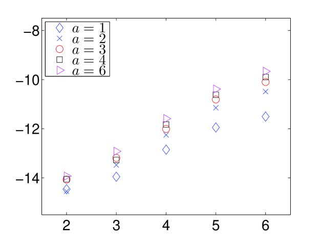
Also, in Figures 1(a), 1(b) we plot the relative errors of $X_{1},Y_{1}$, respectively, on a logarithmic scale as functions of $\log_{10}(c)$. More specifically, each of Figures 1(a), 1(b) contains five plots of such errors, corresponding to $a=1,2,3,4,6$, respectively. Each point on such plot is the geometric mean of ten relative errors (corresponding to ten different values of $\delta$ between 50 and 200). For example, to generate plots corresponding to $a=2$ in Figure 1(a), we use the data from Tables 1–3 (as well as the data corresponding to seven other values of $\delta$).

To each plot in Figures 1(a), 1(b), one can fit a line (in the least square sense). The slopes of such lines are displayed in Table 7. This table has the following structure. Each column corresponds to a different value of $a$. Second row contains the slopes corresponding to $\text{\rm{rel}}(Y_{1})$ (see Figure 1(b)). Third row contains the slopes corresponding to $\text{\rm{rel}}(X_{1})$ (see Figure 1(a)). Fourth row contains $\beta(a)$, where $\beta(a)$ is defined via (229) below (the values in third and fourth rows would be identical if $\text{\rm{rel}}(X_{1})$ were proportional to $c^{\beta(a)}$). Last row contains the number $4\cdot a/(a+2)$ (the power of $c$ in (213) of Theorem 19).

Observations. Several observations can be made from Tables 1–6, Figure 1, Table 7, and some additional numerical experiments by the author.

Observation 1. For every choice of parameters in Experiment 1, the coordinate $X_{1}$ is fairly small compared to $X_{k}$, as predicted by Theorem 3 and Corollary 1 in Section 3.1 (for all $c$, $X_{1}/X_{k}\approx 10^{-25},10^{-50},10^{-75}$ for $\delta=50,100,150$, respectively). Despite this fact, both $X_{1}$ and $Y_{1}$ are still evaluated to fairly high relative accuracy, in all cases.

Observation 3. For any $c$ and $a$, the relative accuracy of both $X_{1}$ and $Y_{1}$ seems to be essentially independent of their magnitude. For example, for $a=4$ and $c=10^{6}$, the relative accuracy of $X_{1}$ is 0.4E-8, 0.6E-8, 0.4E-8 for $\delta=50,100,150$, respectively (despite the fact that $X_{1}$ itself is equal to 0.4E-33, 0.6E-58, 0.1E-85, respectively). In other words, the $\delta$-dependent factor in (213) of Theorem 19 seems to be an artifact of the analysis.

Observation 4. On the other hand, the relative accuracy of both $X_{1}$ and $Y_{1}$ does depend on $c$ (as Theorem 19 suggests). In particular, for any fixed $a$, the relative error of $Y_{1}$ seems to be roughly proportional to $c$, e.g.

$$\text{\rm{rel}}(Y_{1})=O(c)\cdot\varepsilon,$$ (228)

where $\varepsilon$ is the machine precision (see second row in Table 7).

Observation 5. For any fixed $a$, the relative error of $X_{1}$ seems to be roughly proportional to $c^{\beta}$, where $\beta=\beta(a)$ is defined via the formula

$$\beta(a)=\frac{2\cdot a}{a+2}$$ (229)

(see third and fourth rows in Table 7, and also Conjecture 1). On the other hand, in Theorem 19 in Section 3.3 we derived a certain upper bound on the relative error of $X_{1}$ (see (213) and last row in Table 7); this bound is proportional to $c^{4a/(a+2)}$. In other words, numerical experiments seem to indicate that Theorem 19 overestimates the number of lost digits roughly by a factor of two. For example, for $a=4$, $\delta=150$ and $c=10^{6}$ (see last column in Table 6) we lose almost $\beta(a)\cdot 6=8$ decimal digits, while the pessimistic estimate from Theorem 19 suggest that we will lose 16 decimal digits. In other words, the estimate from Theorem 19 is overly cautious.

(a) $\log_{10}(\text{\rm{rel}}(X_{1}))$ as a function of $\log_{10}(c)$.

(b) $\log_{10}(\text{\rm{rel}}(Y_{1}))$ as a function of $\log_{10}(c)$.

Figure 1: Relative errors of $X_{1},Y_{1}$, on a logarithmic scale, as a function of $\log_{10}(c)$, for $a=1,2,3,4,6$. Corresponds to Experiment 1.

6.2 Experiment 2.

In Experiment 1, we took a rather detailed look at relative errors to which the first coordinate of an eigenvector of certain tridiagonal matrices is evaluated. The purpose of this section is to illustrate the analysis of Section 3 in a more qualitative way.

To that end, we carry out the experiment described in Section 6.1 with the following parameters: $a=2$, $c=1000$, $n=1497$, $\delta=50$ (see Table 1). We obtain the four unit-length vectors $X,Y,\hat{X},\hat{Y}$ in $\mathbb{R}^{n}$, as described in Section 6.1.

Figures. We display the results of this experiment in Figures 2(a)–2(c). In each figure, the abscissa corresponds to the indices of the eigenvector, i.e. $1\leq j\leq n$; thus, we plot certain functions of the indices of the eigenvector.

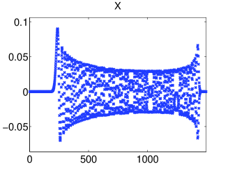
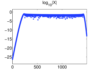
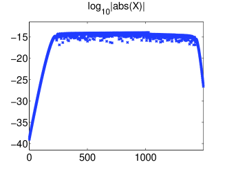
In Figure 2(a), we plot the coordinates $X_{j}$ of $X$, on the linear scale (left) and on the logarithmic scale (right).

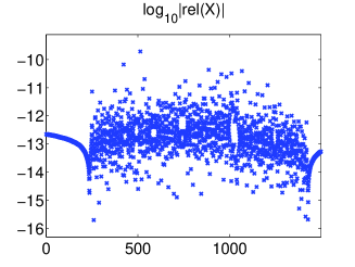
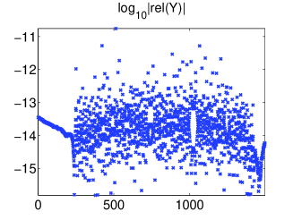
In Figure 2(b), we plot the relative (left) and absolute (right) errors of $X_{j}$ on the logarithmic scale.

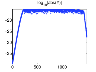
In Figure 2(c), we plot the relative (left) and absolute (right) errors of $Y_{j}$ on the logarithmic scale.

Observations. Several observations can be made from Figures 2(a)–2(c).

The following three observations pertain to the behavior of the coordinates of $X$ (see Figure 2(a)).

Observation 1. In the beginning, the coordinates of $X$ grow rapidly from $\approx 10^{-26}$ to $\approx 10^{-1}$ up to the index $k$ such that $\lambda\approx A_{k}+2$ (in agreement with Theorem 3 in Section 3.1). We refer to the corresponding indices as the ”region of growth”.

Observation 2. At the other end, they decay rapidly (while changing signs) from $\approx 0.05$ to $\approx 10^{-14}$, starting from the index $n-q$ such that $\lambda\approx A_{n-q}-2$ (in agreement with Theorem 4 in Section 3.1). We refer to the corresponding indices as the ”region of decay”.

Observation 3. In the middle (i.e. for indices $j$ such that $\lambda-2\leq A_{j}\leq\lambda+2$), the coordinates behave in an ”oscillatory way” (see e.g. Figure 2(a)). Such behavior is expected from Theorems 7, 8 and Corollaries 3, 4 in Section 3.1. We refer to the corresponding indices as the ”oscillatory region” (see also [16] for an alternative approach to the evaluation of $X_{j}$ in the oscillatory region that, inter alia, further justifies this term).

The following observations pertain to the behavior of relative and absolute errors to which the coordinates of the eigenvector are evaluated, by either Inverse Power or the algorithm from Section 4.3.

Observation 4. Qualitatively, the behavior of relative errors of $X_{j}$ is similar to that of $Y_{j}$ and depends of whether $j$ is in the region of growth, in the region of decay, or in the oscillatory region.

Observation 5. In the region of growth, the relative errors of $X_{j}$ change monotonically with $j$ and always stays ”small” (below $10^{-12}$), in agreement with Theorems 10, 13, Corollary 6 in Section 3.2 and Theorem 19 in Section 3.3. In the region of decay, the relative errors of $X_{j}$ display a similar behavior, in agreement with Theorem 14, Corrolary 6 in Section 3.2, and Theorem 19 in Section 3.3. In particular, both in the regions of growth and in the region of decay the relative errors of $X_{j}$ essentially do not depend on the magnitude of $X_{j}$.

Observation 6. In the oscillatory region, the relative errors of $X_{j}$ oscillate between $10^{-16}$ and $10^{-10}$. On the other hand, the absolute errors of $X_{j}$ always stay below roughly $10^{-14}$. In other words, the relative errors of $X_{j}$ in the oscillatory region depend on the magnitude of $X_{j}$, in agreement with Theorems 12, 13 in Section 3.2.

6.3 Experiment 3.

In this experiment, we illustrate the numerical algorithms of Section 4 via evaluation of Bessel functions (see Sections 2.1, 2.2.2, 5.1).

Description. We first choose, more or less arbitrarily, the real number $\delta\geq 0$. Then, for each choice of five different values $c=10^{2},10^{3},10^{4},10^{5},10^{6}$, we do the following. We define the integer $m=m(\delta,c)$ via the formula

$$m=c+\delta^{2/3}\cdot c^{1/3}$$ (230)

(see (175) in Theorem 17 and (198) in Theorem 18), select the integer $N>m$ (according to Remark 4 in Section 2.2.2), define the integer $n$ via the formula

$$n=2\cdot N+1,$$ (231)

define $A_{1},\dots,A_{n}$ via (209) with $a=1$ in Theorem 19, and then define the symmetric tridiagonal $n\times n$ matrix $A=A(c)$ via (17). Then, we define the real number $\lambda(c)$ via the formula

$$\lambda(c)=2+\frac{n+1}{c}.$$ (232)

(We observe that $\lambda(c)$ is an eigenvalue of $A$, according to (224) in Section 2.2.2.)

Next, we obtain the unit-length $\lambda(c)$-eigenvector of $A$ by four different methods:

1. $Y=(Y_{N},\dots,Y_{0},\dots,Y_{-N})$ via 30 iterations of Shifted Inverse Power, in double precision (observe that the indices vary between $N$ and $-N$, as in (225)).

2. $X=(X_{N},\dots,X_{0},\dots X_{-N})$ via the algorithm from Section 4.3, in double precision.

3. $\hat{Y}=(\hat{Y}_{N},\dots,\hat{Y}_{0},\dots,\hat{Y}_{-N})$ via 30 iterations of Shifted Inverse Power, in extended precision.

4. $\hat{X}=(\hat{X}_{N},\dots,\hat{X}_{0},\dots,\hat{X}_{-N})$ via the algorithm from Section 4.3, in extended precision.

The experiment is conducted for each pair of values $\delta,c$, where $\delta=50,100,150$ and $c=10^{2},10^{3},10^{4},10^{5},10^{6}$. In each case, we verify that each of $\hat{X}$ and $\hat{Y}$ satisfies the definition of an eigenvector coordinate-wise to at least 17 decimal digits, and also that $\hat{X}=\hat{Y}$ to at least 17 decimal digits. In other words, each of $\hat{X},\hat{Y}$ is the unit-length $\lambda(c)-$eigenvector of $A$ defined to full double precision. Also, we verify that the middle $2\cdot m+1$ coordinates of both $\hat{X}$ and $\hat{Y}$ are equal to $J_{m}(c),\dots,J_{0}(c),\dots,J_{-m}(c)$ to at least 17 decimal digits (see Remark 4 in Section 2.2.2). We use these observations to compute the accuracy to which the coordinates $X_{m},\dots,X_{0}$ of $X$ and $Y_{m},\dots,Y_{0}$ of $Y$ approximate $J_{m}(c),\dots,J_{0}(c)$.

The results of the experiment are displayed in Tables 8–10. Each of these tables corresponds to a particular choice $\delta$ in (230), and has the following structure. Each of five columns corresponds to a different value of $c$, between $10^{2}$ and $10^{6}$. The first three rows contain $c$, the integer $m$ defined via (230), and the integer $N>m$ (see Remark 4 in Section 2.2.2). The next two rows contain $J_{m}(c)$ and $J_{c}(c)$. The last two rows contain the relative accuracy to which $X_{m}$ and $Y_{m}$, respectively, approximate $J_{m}(c)$.

Observations. Several observations can be made from Tables 8–10.

Observation 1. For every choice of parameters in Experiment 3, $J_{m}(c)$ is fairly small compared to $J_{c}(c)$, as predicted by Theorem 3 and Corollary 1 in Section 3.1 (for all $c$, $J_{c}(c)\leq 10^{-20},10^{-40},10^{-59}$ for $\delta=50,100,150$, respectively). Despite this fact, both $X_{m}$ and $Y_{m}$ approximate $J_{m}(c)$ to a fairly high relative accuracy, in all cases. Moreover, for any $c$, this accuracy seems to be independent of the magnitude of $J_{m}(c)$ (compare to (213) of Theorem 19; see also Conjecture 1).

Observation 4. On the other hand, the relative accuracy of both $X_{1}$ and $Y_{1}$ does depend on $c$ (as Theorem 19 in Section 3.3 suggests). In particular, for any fixed $a$, the relative error of $Y_{1}$ seems to be roughly proportional to $c^{0.8}$, e.g.

$$\text{\rm{rel}}(Y_{1})=O(c^{0.8})\cdot\varepsilon,$$ (233)

where $\varepsilon$ is the machine precision (see second column in Table 7). Also, the relative error of $X_{1}$ seems to be roughly proportional to $c^{2/3}$ (see Table 7), in agreement with Conjecture 1 above (compare to (213) of Theorem 19).

(a) coordinates: linear and logarithmic scales

(b) principal algorithm: relative and absolute errors

(c) inverse power: relative and absolute errors

Figure 2: The coordinates of $X$ (principal algorithm) and $Y$ (30 iterations of Inverse Power). Parameters: $c=1000$, $n=1500$, $\lambda=\mbox{\text{\rm{0.41022E+01}}}$, $k=226$, $q=65$. Corresponds to Experiment 2.

References

- [1] M. Abramowitz, I. A. Stegun, Handbook of Mathematical Functions with Formulas, Graphs and Mathematical Tables, Dover Publications, 1964.
- [2] W. Barth, R. S. Martin, J. H. Wilkinson, Calculation of the Eigenvalues of a Symmetric Tridiagonal Matrix by the Method of Bisection, Numerische Mathematik 9, 386-393, 1967.
- [3] G. Dahlquist, A. Björk, Numerical Methods, Prentice-Hall Inc., 1974.
- [4] G. J. F. Francis The QR transformation, parts I and II, Computer J. 4, 265-271, 332-345. 1961-2.
- [5] W. J. Givens Numerical computation of the characteristic values of a real symmetric matrix, Technical Report ORNL-1574, Oak Ridge National Laboratory, TX. 1954.
- [6] G. Golub, C. V. Loan, Matrix Computations, Second Edition, Johns Hopkins University Press, Baltimore, 1989.
- [7] I.S. Gradshteyn, I.M. Ryzhik, Table of Integrals, Series, and Products, Seventh Edition, Elsevier Inc., 2007.
- [8] E. Isaacson, H. B. Keller, Analysis of Numerical Methods, New York: Wiley, 1966.
- [9] V. N. Kublanovskaya On some algorithms for the solution of the complete eigenvalue problem, Zh. Vych. Mat. 1, pp. 555-570. 1961.
- [10] H. J. Landau, H. O. Pollak, Prolate spheroidal wave functions, Fourier analysis, and uncertainty - II, Bell Syst. Tech. J. January 65-94, 1961.
- [11] R. Lederman, On the Analytical and Numerical Properties of the Truncated Laplace Transform, Yale CS Technical Report #1490, 2014.
- [12] H. J. Landau, H. Widom, Eigenvalue distribution of time and frequency limiting, J. Math. Anal. Appl. 77, 469-81, 1980.
- [13] J. C. P. Miller, Bessel Functions. Part II, Functions of Positive Integer Order, Cambridge University Press, Cambridge, 1952.
- [14] F. W. J. Olver, Some new asymptotic expansions for Bessel functions of large orders, Proc. Cambridge Philos. Soc. 48 (3), pp. 414–427 (1952).
- [15] A. Osipov, V. Rokhlin, H. Xiao, Prolate Spheroidal Wave Functions of Order Zero, Springer, Applied Mathematical Sciences, Vol. 187 (2013).
- [16] A. Osipov, Evaluation of small elements of the eigenvectors of certain symmetric tridiagonal matrices with high relative accuracy, Yale CS Technical Report #1460, 2012.
- [17] A. Osipov, Certain upper bounds on the eigenvalues associated with prolate spheroidal wave functions, Appl. Comput. Harmon. Anal. (2013), http://dx.doi.org/10.1016/j.acha.2013.03.002.
- [18] A. Osipov, V. Rokhlin, On the evaluation of prolate spheroidal wave functions and associated quadrature rules, Appl. Comput. Harmon. Anal. (2013), http://dx.doi.org/10.1016/j.acha.2013.04.002.
- [19] B. N. Parlett, The symmetric eigenvalue problem, Prentice Hall, Inc. 1980.
- [20] D. Slepian, H. O. Pollak, Prolate spheroidal wave functions, Fourier analysis, and uncertainty - I, Bell Syst. Tech. J. January 43-63, 1961.
- [21] J. Stoer, R. Bulirsch, Introduction to Numerical Analysis, Second Edition, Springer-Verlag, 1993.
- [22] J. H. Wilkinson, Algebraic Eigenvalue Problem, Oxford University Press, New York, 1965.
- [23] H. Xiao, V. Rokhlin, N. Yarvin, Prolate spheroidal wavefunctions, quadrature and interpolation, Inverse Problems, 17(4):805-828, 2001.