Double stochastic resonance in the mean-field $q$-state clock models

Abstract

A magnetic system with a phase transition at temperature $T_{c}$ may exhibit double resonance peaks under a periodic external magnetic field because the time scale matches the external frequency at two different temperatures, one above $T_{c}$ and the other below $T_{c}$. We study the double resonance phenomena for the mean-field $q$-state clock model based on the heat-bath-typed master equation. We find double peaks as observed in the kinetic Ising case ($q=2$) for all $q\geq 4$, but for the three-state clock model ($q=3$), the existence of double peaks is possible only above a certain external frequency since it undergoes a discontinuous phase transition.

I Introduction

From extensive investigations on stochastic resonance *[See; e.g.; ][forageneralreviewonstochasticresonance.]gamma, it is now widely accepted that noise can play a constructive role. A schematic example of a particle in a double-well potential illustrates that the particle can move in a synchronized way with a weak external periodic force, when its average waiting time inside a well, determined by the noise strength, is comparable to the half of the period of the external forcing Gammaitoni et al. (1998). This is what is generally called a time-scale matching condition in studies of stochastic resonance. A particularly interesting model system for stochastic resonance is the kinetic Ising model since it can be regarded as coupled two-state oscillators with many degrees of freedom under thermal fluctuations Néda (1995); *leung2; *brey; *neda3d; Kim et al. (2001a). The probability to flip a spin $j$ from $S_{j}$ to $-S_{j}$ is given by the Glauber dynamics Glauber (1963) as

$$w(S_{j}\rightarrow-S_{j})=\frac{1}{1+\exp\{-\beta[E(S_{1},\ldots,S_{j},\ldots,S_{N})-E(S_{1},\ldots,-S_{j},\ldots,S_{N})]\}},$$ (1)

where $\beta$ is the inverse temperature defined by $\beta\equiv 1/T$ with the Boltzmann constant $k_{B}\equiv 1$, and $N$ is the system size. The energy $E$ is a function of the spin configuration $(S_{1},\ldots,S_{N})$, given by

$$E=-J\sum_{\left<ij\right>}S_{i}S_{j}-h\sum_{i}S_{i},$$

where $J$ is a coupling strength, $\sum_{\left<ij\right>}$ runs over the nearest neighbors, and $h$ is an external magnetic field. If we ignore spin correlations and assume that each spin experiences the mean field of the system, we arrive at the mean-field kinetic Ising model, which has served as an ideal starting point to study exact results on stochastic resonance Leung and Néda (1998); Kim et al. (2001a). This model has been analytically shown that there can be two temperatures where the time-scale matching condition is met, one above the critical temperature $T_{c}$ of the system and the other below $T_{c}$. The reason for this double stochastic resonance is that the intrinsic time scale of the system diverges in both the sides, whether $T$ approaches $T_{c}$ from above or from below, so that the matching with the external frequency can occur on either side. Recently, the similar mechanism of time-scale matching in quantum kinetic Ising model is shown to be responsible for the double resonance peaks in quantum stochastic resonance Han et al. (2012).

A natural extension of the Ising model is the $q$-state clock model, where each spin $\theta$ has an angle among discrete values $2\pi n/q$ where $n=0,\ldots,q-1$. The spin at the $j$th site should now take a vector form as $\bm{S}_{j}=(\cos\theta_{j},\sin\theta_{j})=\left(\cos(2\pi n_{j}/q),\sin(2\pi n_{j}/q)\right)$, and the energy function is accordingly rewritten as

$$E=-J\sum_{\left<ij\right>}\bm{S}_{i}\cdot\bm{S}_{j}-\bm{h}\cdot\sum_{i}\bm{S}_{i},$$

where $\bm{h}=(h_{x},h_{y})$ also takes a vector form. The total magnetization is $\bm{M}=N^{-1}\sum_{i}\bm{S}_{i}$, and its magnitude $M\equiv\left|\bm{M}\right|$ will be used as an order parameter. The Ising model corresponds to the case of $q=2$, and the $XY$ model can be studied by taking the limit of $q\rightarrow\infty$. If we wish to construct a kinetic dynamics for this $q$-state clock model, the probability to update spins such as Eq. (1) for the Ising case is readily obtainable by considering the heat-bath algorithm Loison et al. (2004).

In this work, we check the double stochastic resonance in the $q$-state clock model within the linear response theory. When the external field $\bm{h}$ is parallel to the magnetization vector $\bm{M}$, we find qualitatively the same double-resonance feature for all $q>3$. When the field is perpendicular to $\bm{M}$, however, the response is more complicated, and one of the resonance peaks will disappear as we approach the $XY$-model limit by taking $q\rightarrow\infty$. We will pay particular attention to the case of $q=3$, because the system undergoes a discontinuous phase transition unlike the other values of $q\geq 2$ Kihara et al. (1954). This work is organized as follows. In Sec. II, we derive the equation of motion in terms of $M$ for the general $q$-state clock model. From this equation of motion, we discuss the static phase transitions in Sec. III. Then, Sec. IV examines responses of the system when perturbed by a small amount from the static equilibrium. In Sec. V, we will see how the system under thermal fluctuations responds in a resonant way when the perturbation is given as a periodic magnetic field. Then, we conclude this work in Sec. VI.

II Equation of motion

The master equation describing the probability distribution function $P({\bm{\theta}};t)$ for the spin configuration ${\bm{\theta}}$ at time $t$ can be written as

$$\frac{d}{dt}P({\bm{\theta}};t)=-\sum_{j=1}^{N}\sum_{\theta_{j}^{\prime}}w_{j}(\theta_{j}\rightarrow\theta_{j}^{\prime})P({\bm{\theta}};t)+\sum_{j=1}^{N}\sum_{\theta_{j}^{\prime}}w_{j}(\theta_{j}^{\prime}\rightarrow\theta_{j})P({\bm{\theta}}^{\prime};t),$$ (2)

where ${\bm{\theta}}^{\prime}\equiv\{\theta_{1},\theta_{2},\cdots,\theta_{j}^{\prime},\cdots,\theta_{N}\}$ differs from ${\bm{\theta}}\equiv\{\theta_{1},\theta_{2},\cdots,\theta_{j},\cdots,\theta_{N}\}$ only at one site $j$. In the summations over $\theta_{j}^{\prime}$, note that inclusion of the term for $\theta_{j}^{\prime}=\theta_{j}$ gives null contribution in total, and thus has been included only for convenience. In the heat-bath algorithm, the transition rate is given by

$$w_{j}(\theta_{j}\rightarrow\theta_{j}^{\prime})=Z_{j}^{-1}\exp[\beta F_{j}\cos(\theta_{j}^{\prime}-\phi_{j})],$$

where

$$Z_{j}\equiv\sum_{\theta_{j}}\exp[\beta F_{j}\cos(\theta_{j}-\phi_{j})]$$

with the inverse temperature $\beta$. The local field is defined as

$$F_{j}e^{i\phi_{j}}\equiv\frac{J}{z}\sum_{k\in\Lambda_{j}}e^{i\theta_{k}}+h_{j}$$ (3)

with magnitude $F_{j}$ and phase $\phi_{j}$, where $\Lambda_{j}$ is the set of nearest-neighboring sites of $j$ and $z$ is the coordination number ($z\equiv|\Lambda_{j}|={\rm const}$). We also denote the external local field $h_{j}$ as a complex number so that its real (imaginary) part yields the field in $x$ ($y$) direction. The use of the heat-bath transition rate has a great benefit in calculation since it does not depend on the initial state, i.e., $w_{j}(\theta_{j}\rightarrow\theta_{j}^{\prime})=w_{j}(\theta_{j}^{\prime})$, which enables us to write the master equation (2) as

$$\frac{d}{dt}P({\bm{\theta}};t)=-\sum_{j=1}^{N}P({\bm{\theta}};t)+\sum_{j=1}^{N}\sum_{\theta_{j}^{\prime}}w_{j}(\theta_{j}^{\prime}\rightarrow\theta_{j})P({\bm{\theta}}^{\prime};t).$$ (4)

For an arbitrary single-spin function, denoted by $f(\theta_{l})$, the following equation is derived from the master equation

$$\frac{d}{dt}\left<f(\theta_{l})\right>=-\left<f(\theta_{l})\right>+\left<\frac{\sum_{\theta_{l}}\exp[\beta F_{l}\cos(\theta_{l}-\phi_{l})]f(\theta_{l})}{\sum_{\theta_{l}}\exp[\beta F_{l}\cos(\theta_{l}-\phi_{l})]}\right>,$$ (5)

as explained in Appendix A. When $q=2$, it recovers the kinetic Ising case in Ref. Leung and Néda (1998). For the globally-coupled system with no external field, Eq. (3) simply corresponds to the complex magnetization (we henceforth set $J\equiv 1$)

$$Me^{i\phi}=\frac{1}{N}\sum_{k=1}^{N}e^{i\theta_{k}}$$ (6)

and Eq. (5) turns out to be

$$\frac{d}{dt}\left<f(\theta_{l})\right>=-\left<f(\theta_{l})\right>+\left<\frac{\sum_{\theta_{l}}\exp[\beta M\cos(\theta_{l}-\phi)]f(\theta_{l})}{\sum_{\theta_{l}}\exp[\beta M\cos(\theta_{l}-\phi)]}\right>.$$ (7)

We further use $f(\theta_{l})=e^{i(\theta_{l}-\phi)}$ to get $\left<f(\theta_{l})\right>=(1/N)\left<\sum_{l}e^{i(\theta_{l}-\phi)}\right>=\langle M\rangle$ and

$$\frac{d\left<M\right>}{dt}=-\left<M\right>+\left<\frac{\sum_{\theta_{l}}e^{i(\theta_{l}-\phi)}\exp[\beta M\cos(\theta_{l}-\phi)]}{\sum_{\theta_{l}}\exp[\beta M\cos(\theta_{l}-\phi)]}\right>.$$ (8)

The Hamiltonian of the $q$-state clock model without external field is invariant both under the uniform rotation, i.e., $\theta_{l}\rightarrow\theta_{l}+\phi$, and under the reflection, i.e., $\theta_{l}\rightarrow-\theta_{l}$, which leads to

$$\frac{d\left<M\right>}{dt}=-\left<M\right>+\left<\frac{\sum_{\theta_{l}}\cos\theta_{l}\exp(\beta M\cos\theta_{l})}{\sum_{\theta_{l}}\exp(\beta M\cos\theta_{l})}\right>.$$ (9)

For the globally-coupled system in thermodynamic limit, the mean-field approximation becomes exact and we can drop the average symbols to get

$$\frac{dM}{dt}=-M+\frac{\sum_{\theta_{l}}\cos\theta_{l}\exp(\beta M\cos\theta_{l})}{\sum_{\theta_{l}}\exp(\beta M\cos\theta_{l})}.$$ (10)

III Equilibrium phase transition

Table 1: $A_{qm}=\sum_{n=0}^{q-1}\cos^{m}(2\pi n/q)$ for $m=0,1,\cdots,4$. We also list the critical value of the inverse temperature $\beta_{c}$. For the $q$-state globally-coupled clock model $\beta_{c}=2$ for all $q\geq 4$. See text for details.

	$q=2$	$q=3$	$q=4$	$q\geq 5$
$A_{q0}$	$q$
$A_{q1}$	$0$
$A_{q2}$	2	$q/2$
$A_{q3}$	0	$3/4$	$0$
$A_{q4}$	2	$9/8$	4	$3q/8$
$\beta_{c}$	1	$8\ln 2/3\approx 1.848~{}39$	$2$

We are going to apply the above result in Sec. II to the $q$-state clock model, where $\theta_{l}=2\pi n/q$ with $n=0,\ldots,q-1$ in Eq. (10). In this section, we restrict ourselves to a static situation ($dM/dt=0$) in the absence of the magnetic field ($h=0$). In such a static case, Eq. (10) is interpreted as $0=-\partial\mathcal{F}/\partial M$ with the free energy $\mathcal{F}$, and assumes the following form of a self-consistent equation for $M$:

$$M=\frac{\sum_{n=0}^{q-1}\cos(2\pi n/q)\exp[\beta M\cos(2\pi n/q)]}{\sum_{n=0}^{q-1}\exp[\beta M\cos(2\pi n/q)]}=\frac{\partial\ln Z}{\partial(\beta M)},$$ (11)

where

$$Z\equiv\sum_{n=0}^{q-1}\exp[\beta M\cos(2\pi n/q)]=\sum_{m=0}^{\infty}\frac{(\beta M)^{m}}{m!}A_{qm},$$ (12)

with $A_{qm}\equiv\sum_{n=0}^{q-1}\cos^{m}(2\pi n/q)$. Equation (11) is then expanded in the power of $\beta M$ as

$$M = \frac{A_{q1}+\beta MA_{q2}+\frac{1}{2}\beta^{2}M^{2}A_{q3}+\frac{1}{6}\beta^{3}M^{3}A_{q4}+O(M^{4})}{A_{q0}+\beta MA_{q1}+\frac{1}{2}\beta^{2}M^{2}A_{q2}+\frac{1}{6}\beta^{3}M^{3}A_{q3}+\frac{1}{24}\beta^{4}M^{4}+O(M^{5})}$$

$$= \frac{A_{q1}}{A_{q0}}+\frac{A_{q0}A_{q2}-A^{2}_{q1}}{A^{2}_{q0}}(\beta M)+\frac{2A^{3}_{q1}-3A_{q0}A_{q1}A_{q2}+A^{2}_{q0}A_{q3}}{2A^{3}_{q0}}(\beta M)^{2}$$

$$-\frac{6A^{4}_{q1}-12A_{q0}A^{2}_{q1}A_{q2}+4A^{2}_{q0}A_{q1}A_{q3}-A^{2}_{q0}[A_{q0}A_{q4}-3A^{2}_{q2}]}{6A^{4}_{q0}}(\beta M)^{3}+O(\beta^{4}M^{4}).$$

In Table 1, we list values of $A_{qm}$ for $m\leq 4$. Since $A_{q0}=q$ and $A_{q1}=0$ for $q\geq 1$, the above expansion is further simplified to

$$M=\frac{A_{q2}}{q}(\beta M)+\frac{A_{q3}}{2q}(\beta M)^{2}+\frac{qA_{q4}-3A^{2}_{q2}}{6q^{2}}(\beta M)^{3}+O(\beta^{4}M^{4}).$$ (13)

The second term containing $M^{2}$ is particularly interesting, since it corresponds to the cubic term in $\mathcal{F}$, and thus is responsible for discontinuity of a phase transition Goldenfeld (1993). Its coefficient in this case, $A_{q3}$, vanishes for every integer $q>1$ except $q=3$ (see Table 1). It agrees with our expectation since every mean-field $q$-state clock model undergoes a continuous transition except $q=3$, which can be transformed to the mean-field three-state Potts model with a discontinuous transition Kihara et al. (1954).

III.1 $q\neq 3$

When $q\neq 3$, $A_{q3}=0$ (see Table 1) and Eq. (11) does not have the cubic term:

$$M\approx\frac{A_{q2}}{q}\beta M+\frac{qA_{q4}-3A^{2}_{q2}}{6q^{2}}(\beta M)^{3}$$

From Table 1, $A_{q2}=A_{q4}=2$ for $q=2$, and we find

$$M\approx\beta M-\frac{1}{3}\beta^{3}M^{3},$$

which yields $M\sim(\beta-\beta_{c})^{1/2}$ with $\beta_{c}=1$. For $q=4$, we have $A_{q2}=2$ and $A_{q4}=4$, which yields

$$M\approx\frac{1}{2}\beta M-\frac{1}{24}\beta^{3}M^{3},$$

resulting in $M\sim(\beta-\beta_{c})^{1/2}$ with $\beta_{c}=2$. This agrees with an exact relationship between $q=2$ and $4$ Suzuki (1967). For $q>4$, we have $A_{q2}=q/2$ and $A_{q4}=3q/8$ and we arrive at

$$M\approx\frac{1}{2}\beta M-\frac{1}{16}\beta^{3}M^{3},$$

irrespective of $q$, which means that we always find $M\sim(\beta-\beta_{c})^{1/2}$ with $\beta_{c}=2$ [Fig. 1(a)]. The scaling form of $M$ with respect to the temperature also confirms the mean-field value $1/2$ of the magnetization critical exponent, for all values of $q$ other than three. We finally remark that for the $XY$ model ($q\rightarrow\infty$), we replace the summations in Eq. (11) by integrals as

$$M=\frac{\partial}{\partial(\beta M)}\ln\left(\int d\theta e^{\beta M\cos\theta}\right)=\frac{I_{1}(\beta M)}{I_{0}(\beta M)},$$ (14)

where $I_{n}$ is the modified Bessel function Antoni and Ruffo (1995). It is known that $\beta_{c}=2$ in the limit of $q\rightarrow\infty$ Antoni and Ruffo (1995); Kim et al. (2001b), which is in agreement with the above conclusion of $\beta_{c}=2$ for $q\geq 4$. These are verified by numerical calculations as shown in Fig. 1(a), which are obtained by directly solving Eq. (11) in a numerical way.

III.2 $q=3$

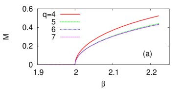
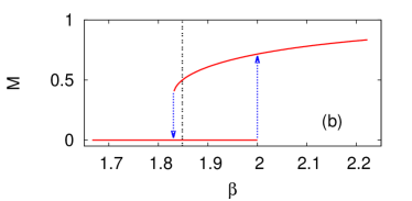
Figure 1: Magnetization of the $q$-state clock model as a function of $T$. (a) $q=4,5,6$, and $7$, which exhibit qualitatively the same behavior as $M\sim|\beta-\beta_{c}|^{1/2}$ with $\beta_{c}=2$. (b) Three-state clock model ($q=3$), exhibiting a discontinuous transition. The bistable region is bounded by $\beta_{1}=2$ and $\beta_{2}\approx 1.830~{}43$ as depicted by the arrows. The vertical dashed line indicates the transition point $\beta_{c}=\frac{8}{3}\ln 2\approx 1.848~{}39$.

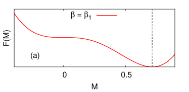
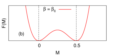
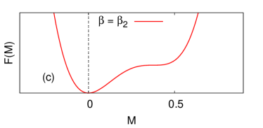
Figure 2: Free-energy landscapes of the three-state clock model as a function of $M$. The free energy ${\mathcal{F}}=M(M+1)/2-\beta^{-1}\log(e^{3\beta M/2}+2)$ is obtained from the integration of Eq. (15). (a) If $\beta\geq\beta_{1}=2$, there exists only one free-energy minimum at nonzero $M$. If $\beta$ is decreased further below $\beta_{1}$, ${\mathcal{F}}$ begins to have two minima, but the global minimum of ${\mathcal{F}}$ occurs at nonzero $M$ for $\beta>\beta_{c}$. (b) At $\beta=\beta_{c}=\frac{8}{3}\ln 2\approx 1.848~{}39$, the two free-energy minima have equal height, one at $M=0$ and the other at $M=1/2$. As $\beta$ is decreased below $\beta_{c}$, the minimum at $M=0$ begins to locate lower than the other minimum at nonzero $M$, but the two minima coexist until $\beta=\beta_{2}$ is reached. (c) When $\beta\leq\beta_{2}\approx 1.830~{}43$, the only minimum is found at $M=0$. Note that the system is bistable for $\beta_{2}<\beta<\beta_{1}$. The vertical dashed lines indicate free-energy minima, and the values of $M$ at these minima are observed in Fig. 1(b).

In the three-state clock model, we observe a discontinuous phase transition due to the cubic term in the expansion of the self-consistent equation (11). However, in order to look into the bistable region in detail, we are not allowed to use the expansion in terms of $\beta M$, since $M$ cannot be assumed to be small in this case. We thus start from Eq. (10) with the equilibrium magnetization $M$ which should satisfy

$$0=-M+\frac{e^{3\beta M/2}-1}{e^{3\beta M/2}+2}.$$ (15)

Let us assume that there exists a certain $\beta$, where the derivative of Eq. (15) with respect to $M$ vanishes. This tells us when bistability becomes possible. Defining $y\equiv e^{3\beta M/2}$, these two conditions can be written as

$$M = \frac{y-1}{y+2},$$

$$\beta = 2y^{-1}(y+2)^{2}/9,$$

which leads to

$$y = \frac{1+2M}{1-M},$$

$$\beta = \frac{2}{(1+2M)(1-M)}.$$ (16)

Inserting these into the definition of $y$, we get a transcendental equation for $M$ as follows:

$$\frac{1}{1-M}-\frac{1}{1+2M}=\ln\left(\frac{1+2M}{1-M}\right).$$ (17)

Note that there is a trivial solution $M_{1}=0$ with $\beta_{1}=2$ from Eq. (16). One can also find a nontrivial solution of Eq. (17) numerically as $M_{2}\approx 0.377~{}201$, and the corresponding inverse temperature is $\beta_{2}\approx 1.830~{}43$. It means that the system is bistable between $\beta_{1}$ and $\beta_{2}$ [Fig. 1(b)]. The transition point $\beta_{c}$ can be determined by checking when the two free-energy minima have an equal height as in the Maxwell construction. Interpreting the left-hand side of Eq. (15) as $\partial\mathcal{F}/\partial M$, we find that $\beta_{c}=\frac{8}{3}\ln 2\approx 1.848~{}39$ (Fig. 2), which is between $\beta_{1}$ and $\beta_{2}$ and in agreement with Refs. Kihara et al. (1954); Mittag and Stephen (1974). One can also readily check that the nonzero magnetization at $\beta_{c}$ is $M=1/2$ by using Eq. (15).

IV Relaxation time

Returning back to the general $q$-state case, the evolution equation of the magnetization vector ($M_{x}$, $M_{y}$) is given by putting $f(\theta_{l})=\cos\theta_{l}$ and $f(\theta_{l})=\sin\theta_{l}$ in Eq. (7) since $M_{x}=\left<\cos\theta_{l}\right>$ and $M_{y}=\left<\sin\theta_{l}\right>$. Within the mean-field scheme with no external field, we find

$$\frac{\displaystyle dM_{x}}{\displaystyle dt}=-M_{x}+\frac{\sum_{\theta}\cos\theta\exp[\beta M\cos(\theta-\phi)]}{\sum_{\theta}\exp[\beta M\cos(\theta-\phi)]}$$

$$\frac{\displaystyle dM_{y}}{\displaystyle dt}=-M_{y}+\frac{\sum_{\theta}\sin\theta\exp[\beta M\cos(\theta-\phi)]}{\sum_{\theta}\exp[\beta M\cos(\theta-\phi)]},$$

where $(M_{x},M_{y})=(M\cos\phi,M\sin\phi)$ from Eq. (6) and $\sum_{\theta}$ runs over $\theta=2\pi n/q$ with $n=1,\ldots,q-1$. We then add perturbation $\bm{\delta}=(\delta_{x},\delta_{y})$ around the equilibrium magnetization with the assumption $\beta|\bm{\delta}|\ll 1$. By expanding the exponential functions and leaving linear terms with respect to $\beta\delta_{x}$ or $\beta\delta_{y}$, one can study linear responses of the system. Without loss of generality, we may set the initial magnetization along the $x$-axis, i.e., $\bm{M}^{\ast}=(M_{x}^{\ast},M_{y}^{\ast})=(M^{\ast},0)$, where $M^{\ast}$ satisfies Eq. (11) as

$$M^{\ast} = \frac{\sum_{\theta}\cos\theta\exp(\beta M^{\ast}\cos\theta)}{\sum_{\theta}\exp(\beta M^{\ast}\cos\theta)},$$

$$0 = \frac{\sum_{\theta}\sin\theta\exp(\beta M^{\ast}\cos\theta)}{\sum_{\theta}\exp(\beta M^{\ast}\cos\theta)}.$$

The linearized equations for perturbation $\delta_{x}(t)=M_{x}(t)-M_{x}^{\ast}$ and $\delta_{y}(t)=M_{y}(t)-M_{y}^{\ast}$ are derived in Appendix B as follows:

$$\frac{d\delta_{x}}{dt} = -\left(1+\beta{M^{\ast}}^{2}-\beta C\right)\delta_{x},$$ (18)

$$\frac{d\delta_{y}}{dt} = -\left(1-\beta+\beta C\right)\delta_{y},$$ (19)

where

$$C\equiv\frac{\sum_{\theta}\cos^{2}\theta\exp(\beta M^{\ast}\cos\theta)}{\sum_{\theta}\exp(\beta M^{\ast}\cos\theta)}.$$ (20)

In other words, we have two relaxation times $\tau_{\parallel}$ and $\tau_{\perp}$ in the parallel and perpendicular directions with respect to the equilibrium magnetization vector, respectively, which are given as

$$\tau_{\parallel}^{-1} = 1+\beta{M^{\ast}}^{2}-\beta C,$$ (21)

$$\tau_{\perp}^{-1} = 1-\beta+\beta C=2+\beta({M^{\ast}}^{2}-1)-\tau_{\parallel}^{-1}.$$ (22)

Very near to the critical point, we may assume that $M^{\ast}\approx 0$, and we get $C=\sum_{\theta}\cos^{2}\theta/\sum_{\theta}1=A_{q2}/A_{q0}$ (see Table 1). When $q=2$, the $y$ component of magnetization is not defined, and we have $C=A_{22}/A_{20}=1$ from Table 1, yielding $\tau_{\parallel}^{-1}=1-\beta$. For $q>2$, we instead have $C=1/2$ from Table 1, and $\tau_{\parallel}^{-1}=\tau_{\perp}^{-1}=1-\beta/2$. Consequently, the divergence of the relaxation time occurs when $\beta=1$ for $q=2$, and when $\beta=2$ for $q>2$ ($q\neq 3$), in complete agreement with $\beta_{c}=1$ for $q=2$ and $\beta_{c}=2$ for $q>2$ (except for $q=3$ in which $M^{\ast}\approx 0$ is not justified) found in Sec. III.1. Also, the divergence of the relaxation time in the form of $\tau\sim|\beta-\beta_{c}|^{-1}$, determines the dynamic critical exponent $z=2$ in the scaling form $\tau\sim\xi^{z}$, since the correlation-length ($\xi$) exponent $\nu=1/2$ in $\xi\sim|\beta-\beta_{c}|^{-\nu}$ for the mean-field universality class.

IV.1 $q\neq 3$

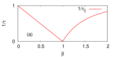
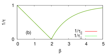
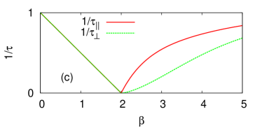
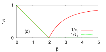
Figure 3: Inverse relaxation times for the $q$-state clock models. (a) $q=2$, (b) $q=4$, (c) $q=5$, and (d) the $XY$ limit ($q\rightarrow\infty$) where $\tau_{\perp}^{-1}\rightarrow 0$ above $\beta_{c}=2$.

As mentioned above, $\tau_{\perp}$ becomes meaningless for the Ising case ($q=2$), and we get $\tau_{\parallel}^{-1}=1+\beta{M^{\ast}}^{2}-\beta$, recovering the result in Refs. Leung and Néda (1998); Kim et al. (2001a) [Fig. 3(a)]. For different values of $q$, we plot Eqs. (21) and (22) in Fig. 3 by solving Eq. (11). For $q=4$, we find $\tau_{\parallel}=\tau_{\perp}$ in the entire region of $T$ [Fig. 3(b)] since

$$C=\frac{e^{\beta M^{\ast}}+e^{-\beta M^{\ast}}}{e^{\beta M^{\ast}}+e^{-\beta M^{\ast}}+2}=1+\left(\frac{e^{\beta M^{\ast}}-1}{e^{\beta M^{\ast}}+1}\right)^{2}=1+{M^{\ast}}^{2}.$$

For $q>4$, we instead observe $\tau_{\perp}\geq\tau_{\parallel}$ at $\beta>\beta_{c}$ [Fig. 3(c)] and the difference becomes pronounced as $q$ increases. In the limiting case of $q\rightarrow\infty$, $\tau_{\perp}$ diverges at $\beta>\beta_{c}$, which reflects the $U(1)$ symmetry of the system. This shows the following identity of the modified Bessel function for $\beta\geq 2$,

$$C=\frac{1}{2}\left[1+\frac{I_{2}(\beta M^{\ast})}{I_{0}(\beta M^{\ast})}\right]=1-\frac{1}{\beta}$$

where $M^{\ast}$ satisfies Eq. (14). This observation is also related to the idea in Ref. Baek et al. (2009) that fluctuations in the angular direction can distinguish the discrete symmetry in the clock model from the continuous symmetry of the $XY$ model.

IV.2 $q=3$

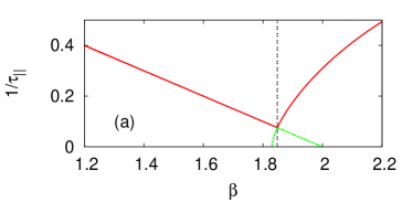
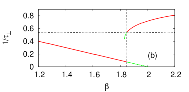
Figure 4: Three-state clock model. (a) Inverse relaxation time $\tau_{\parallel}^{-1}$ in the direction of magnetization and (b) $\tau_{\perp}^{-1}$ in the perpendicular direction. The solid lines represent values at the lowest free energy, while the dotted lines mean what one can observe at metastable states. The vertical dashed lines indicate the transition point $\beta_{c}=\frac{8}{3}\ln 2\approx 1.848~{}39$. The horizontal dashed line shows $1-\frac{2}{3}\ln 2\approx 0.537~{}902$.

As explained above, this system has a bistable region between $\beta_{1}=2$ and $\beta_{2}\approx 1.830~{}43$. Even though the relaxation times can be expressed in the same way, one should note that they are defined in the linear-response regime. In other words, even if the system becomes bistable, the relaxation here means returning back to the original state and not jumping to the other state. If $M^{\ast}=0$, we have seen that $\tau_{\parallel}^{-1}=\tau_{\perp}^{-1}=1-\beta/2$. So both of them vanish if $\beta\rightarrow\beta_{1}^{-}$ from below with keeping $M^{\ast}=0$. If $\beta$ approaches $\beta_{2}$ from above with keeping $M^{\ast}\neq 0$, on the other hand, we find

$$\tau_{\parallel}^{-1}(\beta\rightarrow\beta_{2}^{+})=1-\frac{\beta_{2}}{2}-\frac{\beta_{2}M_{2}}{2}+\beta_{2}M_{2}^{2}=0,$$

by using Eq. (16). Here $M_{2}$ means the nontrivial solution of Eq. (17). These results are plotted in Fig. 4(a). One can clearly see why those metastable branches cannot be sustained beyond $\beta_{1}$ and $\beta_{2}$, respectively. The other inverse relaxation time $\tau_{\perp}^{-1}$ is plotted in Fig. 4(b). Note the jump at $\beta_{c}$ from $\tau_{\perp}^{-1}(\beta\rightarrow\beta_{c}^{-})=1-\beta_{c}/2=1-\frac{4}{3}\ln 2\approx 0.075~{}803~{}8$ to $\tau_{\perp}^{-1}(\beta\rightarrow\beta_{c}^{+})=1-\frac{2}{3}\ln 2\approx 0.537~{}902$. The latter value is obtained by using Eq. (22) with $M^{\ast}=1/2$. This behavior is in accordance with the general tendency that $\tau_{\perp}$ increases in the ordered phases as $q$ becomes larger, but manifests itself in a discontinuous way.

V Resonance

If there exists a uniform external field $\bm{h}=(h_{x},h_{y})$, the evolution equations are generalized to

$$\frac{\displaystyle dM_{x}}{\displaystyle dt}=-M_{x}+\frac{\sum_{\theta}\cos\theta\exp[\beta F\cos(\theta-\phi)]}{\sum_{\theta}\exp[\beta F\cos(\theta-\phi)]}$$ (23)

$$\frac{\displaystyle dM_{y}}{\displaystyle dt}=-M_{y}+\frac{\sum_{\theta}\sin\theta\exp[\beta F\cos(\theta-\phi)]}{\sum_{\theta}\exp[\beta F\cos(\theta-\phi)]},$$ (24)

where $(F\cos\phi,F\sin\phi)=(M_{x}+h_{x},M_{y}+h_{y})$ [see Eq. (3) for globally-coupled ($z=N$) model with a uniform external field]. The magnetization is again decomposed into $(M_{x},M_{y})=(M_{x}^{\ast}+\delta_{x},M_{y}^{\ast}+\delta_{y})$, where we set again $M_{x}^{\ast}=M^{\ast}$ and $M_{y}^{\ast}=0$ as before. Let us furthermore assume that $\beta|\bm{h}|\ll 1$ and expand the equations up to the linear order. The derivation is almost the same as what we did for Eqs. (18) and (19), except that we have to replace $\delta_{x}$ by $\delta_{x}+h_{x}$ as well as $\delta_{y}$ by $\delta_{y}+h_{y}$ in expanding the second terms of Eqs. (23) and (24). This results in

$$\frac{d\delta_{x}}{dt} = -\delta_{x}-\beta\left({M^{\ast}}^{2}-C\right)(\delta_{x}+h_{x})$$

$$= -\tau_{\parallel}^{-1}(\delta_{x}+h_{x})+h_{x}$$

$$= -\tau_{\parallel}^{-1}\delta_{x}+(1-\tau_{\parallel}^{-1})h_{x},$$

$$\frac{d\delta_{y}}{dt} = -\delta_{y}+\beta\left(1-C\right)(\delta_{y}+h_{y})$$

$$= -\tau_{\perp}^{-1}(\delta_{y}+h_{y})+h_{y}$$

$$= -\tau_{\perp}^{-1}\delta_{y}+(1-\tau_{\perp}^{-1})h_{y},$$

where $\tau_{\parallel}^{-1}$ and $\tau_{\perp}^{-1}$ are given by Eqs. (21) and (22). Since these equations have basically the same form, we may drop the subscript $\parallel$ or $\perp$ in finding the formal solution. If we set $h=h_{0}\cos\omega t$, the resulting equation is the following:

$$\frac{d\delta}{dt}=-\tau^{-1}\delta+(1-\tau^{-1})h_{0}\cos\omega t.$$ (25)

Its solution is obtained by assuming

$$\delta(t)=\delta_{0}\cos(\omega t-\sigma),$$

which results in phase shift $\sigma=\arctan(\omega\tau)$ and amplitude

$$\delta_{0}=\frac{(\tau-1)h_{0}}{\sqrt{1+\omega^{2}\tau^{2}}}.$$

We can interpret this solution as follows. When $\tau\sim O(1)$, the left-hand side of Eq. (25) is negligible compared to the first term of the right-hand side since $\omega\ll 1$ by assumption. Then, $\delta$ becomes directly proportional to $h_{0}\cos\omega t$ without any phase shift, even though the amplitude will be small. On the other hand, if $\tau\gg 1$, the first term on the right-hand side of Eq. (25) becomes negligible so that $d\delta/dt$ is proportional to $h_{0}\cos\omega t$, which leads to a phase shift of $\pi/2$ in $\delta(t)$ compared to the magnetic field.

The ac susceptibility components are defined as

$$\chi^{\prime} = \frac{1}{\pi h_{0}}\int_{0}^{2\pi}d(\omega t)~{}M\cos\omega t,$$

$$\chi^{\prime\prime} = \frac{1}{\pi h_{0}}\int_{0}^{2\pi}d(\omega t)~{}M\sin\omega t.$$

The former one $\chi^{\prime}$ is closely related to the occupancy ratio used in Ref. Kim et al. (2001a) to measure how many spins are aligned in the direction of the external field. By inserting $\delta(t)$ here, we obtain

$$\chi^{\prime} = \frac{\tau-1}{1+\omega^{2}\tau^{2}},$$ (26)

$$\chi^{\prime\prime} = \frac{\omega\tau(\tau-1)}{1+\omega^{2}\tau^{2}}=\omega\tau\chi^{\prime},$$ (27)

where the static value $M^{\ast}$ integrates out to zero when multiplied by the sinusoidal functions. When $M^{\ast}=0$ and $\tau^{-1}=1-\beta/2$, the maximum of Eq. (26) is found at $\beta=2\omega^{2}+2-2\omega\sqrt{\omega^{2}+1}$, which approaches unity as $\omega\rightarrow\infty$. In general, the extremum condition of $\chi^{\prime}$ with respect to $\beta$ is equivalent to $2\omega\chi^{\prime\prime}=1$ since

$$\frac{d\chi^{\prime}}{d\beta}=\frac{d\tau/d\beta}{1+\omega^{2}\tau^{2}}-\frac{\tau-1}{(1+\omega^{2}\tau^{2})^{2}}2\omega^{2}\tau\frac{d\tau}{d\beta}=\left(\frac{d\tau}{d\beta}\right)\frac{1-2\omega\chi^{\prime\prime}}{1+\omega^{2}\tau^{2}}.$$

This condition yields a solution $\omega=(\tau^{2}-2\tau)^{-1/2}$, which can be expanded as $\tau^{-1}+\tau^{-2}+\frac{3}{2}\tau^{-3}+\cdots$. Therefore, the optimal frequency $\omega$ for resonance coincides with $\tau^{-1}$ to the leading order when $\tau\gg 1$. Consequently, the stochastic resonance occurs when the extrinsic time scale $1/\omega$ matches with the intrinsic one $\tau$ Gammaitoni et al. (1998); Kim et al. (2001a).

V.1 $q\neq 3$

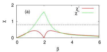
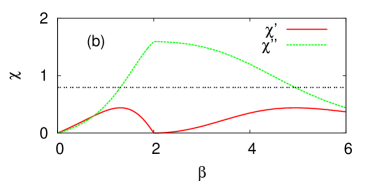
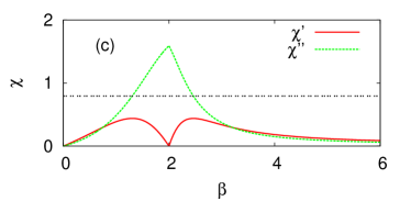
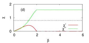
Figure 5: ac susceptibility components for $q=6$ given by Eqs. (26) and (27) with $\omega=2\pi\times 10^{-1}$. (a) The field can be exerted in the $x$ direction or (b) in the $y$ direction. The next two panels show the same plots for $q\rightarrow\infty$, with (c) the field in the $x$ direction and (d) in the $y$ direction. The horizontal dashed lines indicate $\chi^{\prime\prime}=(2\omega)^{-1}$ to locate the maxima in $\chi^{\prime}$.

First, we consider the field in the $x$ direction, parallel to the magnetization. We thus use $\tau_{\parallel}$ in place of $\tau$ in Eqs. (26) and (27). If the system undergoes a continuous phase transition with $q\neq 3$, one can clearly see two peaks in $\chi^{\prime}$ above and below $\beta_{c}$. We show the case of $q=6$ in Fig. 5(a), noting that qualitatively the same behavior is observed for other $q$ values. Now let us apply the field in the $y$ direction for $q\neq 2$ (note that the field in $y$ direction for $q=2$ is meaningless). When $\beta<\beta_{c}$, the disordered phase of the system is isotropic so we observe the same response as above, although the field direction has changed. However, when $\beta>\beta_{c}$, the peak is suppressed to a higher $\beta$ [Fig. 5(b)]. As $q\rightarrow\infty$, $\chi^{\prime}$ eventually vanishes and $\chi^{\prime\prime}$ becomes constant at $\beta>\beta_{c}$, which signals the $U(1)$ symmetry [Fig. 5(d)].

V.2 $q=3$

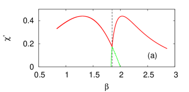
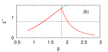
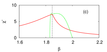
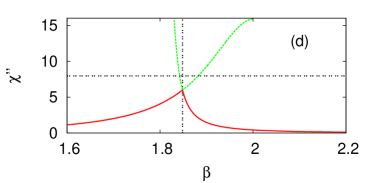
Figure 6: Three-state clock model under the field in the $x$ direction. (a)-(b) ac susceptibilities at $\omega=2\pi\times 10^{-1}$ and (c)-(d) the same quantities but at $\omega=2\pi\times 10^{-2}$. The solid lines represent values at the lowest free energy, while the dotted lines mean what one can observe at metastable states. The vertical dashed lines indicate the transition point $\beta_{c}=\frac{8}{3}\ln 2\approx 1.848~{}39$. The horizontal dashed lines indicate $(2\omega)^{-1}$.

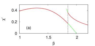
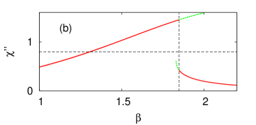
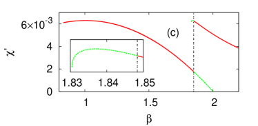
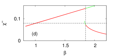
Figure 7: Three-state clock model under the field in the $y$ direction. (a)-(b) ac susceptibilities at $\omega=2\pi\times 10^{-1}$ and (c)-(d) the same quantities but at $\omega=2\pi$. Inset: a zoomed view of the left branch, showing a maximum around $\beta\approx 1.837$. The solid lines represent values at the lowest free energy, while the dotted lines mean what one can observe at metastable states. The vertical dashed lines indicate the transition point $\beta_{c}=\frac{8}{3}\ln 2\approx 1.848~{}39$. The horizontal dashed lines indicate $(2\omega)^{-1}$.

When the field is parallel to the magnetization, one can infer from Fig. 4(a) the possibility of two resonance peaks only above a certain frequency since one can find two temperatures where the external frequency matches the relaxation time scale only if $\tau^{-1}>1-\beta_{c}/2\approx 0.075~{}803~{}8$. One cannot find proper relaxation time scales to match the external driving frequency if the frequency is too low. It is readily confirmed in Figs. 6(a) to 6(d). More precisely, the threshold of $\omega$ for the stable double resonance peaks can be found by requiring $\chi^{\prime\prime}=(2\omega)^{-1}$ to be met exactly at $\beta=\beta_{c}=\frac{8}{3}\ln 2$. Since $\tau_{\parallel}^{-1}(\beta_{c})=1-\beta_{c}/2$, we get the following quadratic equation,

$$\frac{\omega\tau_{\parallel}(\tau_{\parallel}-1)}{1+\omega^{2}\tau_{\parallel}^{2}}=\frac{1}{2\omega},$$ (28)

which yields $\omega=(3-4\ln 2)/\sqrt{24\ln 2-9}\approx 0.0822986$.

When the field is perpendicular to the magnetization, one can guess that the external frequency $\omega$ should be again large enough to find two matching temperatures. In Fig. 4(b), for example, the minimum $\tau_{\perp}^{-1}$ above which there stably exist two matching temperatures is found to be $\tau_{\perp}^{-1}=1-\frac{2}{3}\ln 2\approx 0.537~{}902$. It is true that one finds only one maximum in $\chi^{\prime}$ when $\omega$ is low [Figs. 7(a) and (b)]. However, our calculation shows that the double resonance is anyway impossible if we take only truly stable states into account. The left maximum in $\chi^{\prime}$ can be located only on a metastable branch even for a very large value of $\omega$ [Figs. 7(c)]. If we repeat the same calculation as Eq. (28) to find the threshold of $\omega$ with $\tau_{\perp}^{-1}=1-\frac{2}{3}\ln 2$, we indeed find that the equation does not possess any real solution, confirming this impossibility.

VI Summary

In summary, we have studied stochastic resonance with the mean-field kinetic version of the $q$-state clock model. The response under a periodic external field now depends on the direction of the field relative to the magnetization vector. When they are parallel, the double stochastic resonance is observed for every $q>3$ qualitatively in the same way as in the kinetic Ising case ($q=2$) Kim et al. (2001a). When the field is perpendicular to the magnetization vector, on the other hand, the resonance peak is suppressed to a lower temperature and eventually vanishes as $q\rightarrow\infty$ since the $U(1)$ symmetry sets in. For $q=3$, the discontinuous transition should be also taken into account, and we have concluded that the double resonance peaks are observable in a truly stable manner only when the external driving frequency is high enough and the field direction is parallel to that of the magnetization vector.

Appendix A Derivation of Eq. (5)

We multiply each side of Eq. (4) by an arbitrary function of spin $l$, denoted by $f(\theta_{l})$, and carry out summation over all the possible configurations:

$$\sum_{\bm{\theta}}\frac{d}{dt}P({\bm{\theta}};t)f(\theta_{l})=-\sum_{\bm{\theta}}\sum_{j=1}^{N}P({\bm{\theta}};t)f(\theta_{l})+\sum_{\bm{\theta}}\sum_{j=1}^{N}\sum_{\theta_{j}^{\prime}}w_{j}(\theta_{j}^{\prime}\rightarrow\theta_{j})P({\bm{\theta}}^{\prime};t)f(\theta_{l}).$$ (29)

The sum over $j$ is decomposed into two parts: the sum over terms with $j\neq l$ and the term for $j=l$. Let us consider the former first. If we write $\theta_{j}^{\prime}=\theta_{j}+\Delta$, we get

$$-\sum_{\bm{\theta}}\sum_{j\neq l}^{N}P({\bm{\theta}};t)f(\theta_{l})+\sum_{\bm{\theta}}\sum_{j\neq l}^{N}\sum_{\Delta}w_{j}(\theta_{j})P(\theta_{1},\cdots,\theta_{j}+\Delta,\cdots,\theta_{N};t)f(\theta_{l})$$

$$= -\sum_{\bm{\theta}}\sum_{j\neq l}^{N}P({\bm{\theta}};t)f(\theta_{l})+\sum_{\bm{\theta}}\sum_{j\neq l}^{N}\sum_{\Delta}w_{j}(\theta_{j}-\Delta)P({\bm{\theta}};t)f(\theta_{l})=0,$$

where $\sum_{\theta_{j}^{\prime}}w_{j}(\theta_{j}^{\prime})=1$ has again been used. With $\langle f(\theta_{l})\rangle\equiv\sum_{\bm{\theta}}P({\bm{\theta}};t)f(\theta_{l})$ and $\theta_{l}^{\prime}=\theta_{l}+\Delta$ again, Eq. (29) is now reduced to

$$\frac{d}{dt}\left<f(\theta_{l})\right> = -\left<f(\theta_{l})\right>+\sum_{\bm{\theta}}\sum_{\Delta}w_{l}(\theta_{l})P(\theta_{1},\cdots,\theta_{l}+\Delta,\cdots,\theta_{N};t)f(\theta_{l})$$

$$= -\left<f(\theta_{l})\right>+\sum_{\bm{\theta}}\sum_{\Delta}w_{l}(\theta_{l}-\Delta)P({\bm{\theta}};t)f(\theta_{l}-\Delta)$$

$$= -\left<f(\theta_{l})\right>+\left<\sum_{\Delta}w_{l}(\theta_{l}-\Delta)f(\theta_{l}-\Delta)\right>$$

$$= -\left<f(\theta_{l})\right>+\left<\frac{\sum_{\Delta}\exp[\beta F_{l}\cos(\theta_{l}-\phi_{l}-\Delta)]f(\theta_{l}-\Delta)}{\sum_{\theta_{l}}\exp[\beta F_{l}\cos(\theta_{l}-\phi_{l})]}\right>$$

$$= -\left<f(\theta_{l})\right>+\left<\frac{\sum_{\theta_{l}}\exp[\beta F_{l}\cos(\theta_{l}-\phi_{l})]f(\theta_{l})}{\sum_{\theta_{l}}\exp[\beta F_{l}\cos(\theta_{l}-\phi_{l})]}\right>.$$

Appendix B Derivation of Eqs. (18) and (19)

The perturbation in $M_{x}$ is expanded up to the first order as follows:

$$\frac{d\delta_{x}}{dt} = -M_{x}^{\ast}-\delta_{x}+\frac{\sum_{\theta}\cos\theta~{}e^{\beta M_{x}\cos\theta}e^{\beta M_{y}\sin\theta}}{\sum_{\theta}e^{\beta M_{x}\cos\theta}e^{\beta M_{y}\sin\theta}}$$

$$= -M^{\ast}-\delta_{x}+\frac{\sum_{\theta}\cos\theta~{}e^{\beta M^{\ast}\cos\theta}e^{\beta\delta_{x}\cos\theta}e^{\beta\delta_{y}\sin\theta}}{\sum_{\theta}e^{\beta M^{\ast}\cos\theta}e^{\beta\delta_{x}\cos\theta}e^{\beta\delta_{y}\sin\theta}}$$

$$\approx -M^{\ast}-\delta_{x}+\frac{\sum_{\theta}\cos\theta~{}e^{\beta M^{\ast}\cos\theta}(1+\beta\delta_{x}\cos\theta+\beta\delta_{y}\sin\theta)}{\sum_{\theta}e^{\beta M^{\ast}\cos\theta}(1+\beta\delta_{x}\cos\theta+\beta\delta_{y}\sin\theta)}$$

$$= -M^{\ast}-\delta_{x}+\frac{\sum_{\theta}\cos\theta~{}e^{\beta M^{\ast}\cos\theta}+\sum_{\theta}\cos\theta~{}e^{\beta M^{\ast}\cos\theta}(\beta\delta_{x}\cos\theta+\beta\delta_{y}\sin\theta)}{\sum_{\theta}e^{\beta M^{\ast}\cos\theta}+\sum_{\theta}e^{\beta M^{\ast}\cos\theta}(\beta\delta_{x}\cos\theta+\beta\delta_{y}\sin\theta)}$$

$$\approx -M^{\ast}-\delta_{x}+\left\{\sum_{\theta}\cos\theta~{}e^{\beta M^{\ast}\cos\theta}+\sum_{\theta}\cos\theta~{}e^{\beta M^{\ast}\cos\theta}(\beta\delta_{x}\cos\theta+\beta\delta_{y}\sin\theta)\right\}$$

$$\times\left\{\sum_{\theta}e^{\beta M^{\ast}\cos\theta}-\sum_{\theta}e^{\beta M^{\ast}\cos\theta}(\beta\delta_{x}\cos\theta+\beta\delta_{y}\sin\theta)\right\}\times\left\{\sum_{\theta}e^{\beta M^{\ast}\cos\theta}\right\}^{-2}$$

$$= -\delta_{x}-\left\{\sum_{\theta}\cos\theta~{}e^{\beta M^{\ast}\cos\theta}\sum_{\theta}e^{\beta M^{\ast}\cos\theta}(\beta\delta_{x}\cos\theta+\beta\delta_{y}\sin\theta)\right\}\times\left\{\sum_{\theta}e^{\beta M^{\ast}\cos\theta}\right\}^{-2}$$

$$+\left\{\sum_{\theta}e^{\beta M^{\ast}\cos\theta}\sum_{\theta}\cos\theta~{}e^{\beta M^{\ast}\cos\theta}(\beta\delta_{x}\cos\theta+\beta\delta_{y}\sin\theta)\right\}\times\left\{\sum_{\theta}e^{\beta M^{\ast}\cos\theta}\right\}^{-2}$$

$$= -\delta_{x}-\beta{M^{\ast}}^{2}\delta_{x}+\frac{\sum_{\theta}\cos\theta\exp(\beta M^{\ast}\cos\theta)(\beta\delta_{x}\cos\theta+\beta\delta_{y}\sin\theta)}{\sum_{\theta}\exp(\beta M^{\ast}\cos\theta)}.$$

Likewise, we obtain

$$\frac{d\delta_{y}}{dt}=-\delta_{y}+\frac{\sum_{\theta}\sin\theta\exp(\beta M^{\ast}\cos\theta)(\beta\delta_{x}\cos\theta+\beta\delta_{y}\sin\theta)}{\sum_{\theta}\exp(\beta M^{\ast}\cos\theta)}.$$

One can furthermore show that

$$\sum_{\theta}\cos\theta\sin\theta\exp(\beta M^{\ast}\cos\theta)=0,$$

by which we can rewrite the above equations as

$$\frac{d\delta_{x}}{dt} = -\left(1+\beta{M^{\ast}}^{2}-\beta C\right)\delta_{x},$$

$$\frac{d\delta_{y}}{dt} = -\left(1-\beta+\beta C\right)\delta_{y},$$

where

$$C\equiv\frac{\sum_{\theta}\cos^{2}\theta\exp(\beta M^{\ast}\cos\theta)}{\sum_{\theta}\exp(\beta M^{\ast}\cos\theta)}.$$