The Effect of Macrodiversity on the Performance of Maximal Ratio Combining in Flat Rayleigh Fading

Abstract

The performance of maximal ratio combining (MRC) in Rayleigh channels with co-channel interference (CCI) is well-known for receive arrays which are co-located. Recent work in network MIMO, edge-excited cells and base station collaboration is increasing interest in macrodiversity systems. Hence, in this paper we consider the effect of macrodiversity on MRC performance in Rayleigh fading channels with CCI. We consider the uncoded symbol error rate (SER) as our performance measure of interest and investigate how different macrodiversity power profiles affect SER performance. This is the first analytical work in this area. We derive approximate and exact symbol error rate results for $M$-QAM/BPSK modulations and use the analysis to provide a simple power metric. Numerical results, verified by simulations, are used in conjunction with the analysis to gain insight into the effects of the link powers on performance.

I Introduction

Maximum ratio combining (MRC) is a well-known linear combining technique that maximizes the signal-to-noise ratio (SNR) in noise limited systems [1]. In the presence of co-channel interferers, MRC is sub-optimal compared to minimum mean squared error (MMSE) combining. However, MMSE combining requires instantaneous channel knowledge of both the desired source and interfering sources. In contrast, MRC only requires a knowledge of the desired source and hence is simpler to implement. For this reason, there is still interest in MRC processing in the presence of interference. In [2], MRC is investigated for large systems where it was shown that in the limit as the number of antennas increases, intercell interference effects disappear. In [3], a switched MRC/MMSE receiver is proposed where the simplicity of MRC is preferred when the interference levels drop below a threshold. Here, MRC performance in the presence of small but non-zero interference is important. There are well-known methods to estimate the interference level in comparison with the signal level as described in [4].
The performance of MRC systems with co-located antenna arrays is well known for Rayleigh fading channels with multiple co-channel interferers [5, 6]. Recently, interest in distributed combining has grown due to research in cooperative systems, base-station collaboration [7, pp. 69], edge-excited cells [8, 9] and network MIMO [10, 11]. In the standards, distributed processing is part of coordinated multipoint transmission (CoMP) in LTE Advanced. For these macrodiversity systems, every link may have a different average SNR since the sources and the receive antennas are all in different locations. This variation in SNR makes performance analysis more complex and to the best of our knowledge no analytical results are currently available for such systems.
Hence, in this paper we analyze the symbol-error-rate (SER) of macrodiversity MRC systems. Note that the system is not new. Standard MRC processing is considered and so the general form of the receiver output and the initial steps in the performance evaluation are well-known. However the macrodiversity layout creates a new channel structure which is far more complex than the microdiversity channel. Hence, the MRC output has a completely new statistical distribution and a novel, more advanced analysis is required for system performance evaluation. In particular, we consider a distributed antenna array performing MRC combining for a single antenna desired source in the presence of an arbitrary number of single antenna co-channel interferers. The analysis also covers the case where both the desired and interfering sources may have multiple antennas. Since the sources and the receive antennas are not co-located, the channels are normally independent and so the focus is on independent Rayleigh fading channels where each link has a different SNR. In this paper, we evaluate the SER over Rayleigh fading for fixed values of the long term link SNRs. Hence, the SER is computed over fast fading while path loss effects and shadowing are held constant. Looking at the joint effects of the slow fading (see, for example, [12, 13]) would be an interesting topic for future work. In the scenario where some sources have multiple antennas, there may be spatial correlation in the channels corresponding to the antennas at that source. However, this is beyond the scope of the current work where independent channels are considered. We provide specific results for BPSK and QPSK modulations, but the analysis can be applied to $M$-QAM and a wide range of modulations where the SER can be written in terms of an expected value of the Gaussian $Q$-function and $Q^{2}$-function. The general analytical approach follows the techniques in [14]. The novelty in the analysis is the identification of a representation for the interference and noise term in the combiner output and the use of this representation in exact SER calculations. We then use the SER results to analyze the effect of macrodiversity on MRC performance.

The rest of the paper is organized as follows. In Sec. II, we give the system model and in Sec. III the performance results and SER are derived. Sec. IV gives numerical results where the analysis is verified by simulation and conclusions are presented in Sec. V.

II System Model

Consider $N$ single-antenna distributed users communicating with $n_{R}$ distributed transmission points (TP) [16] each with a single receive antenna over an independent flat fading Rayleigh channel. The system diagram is given in Fig.1. The received signal is given by

$$r = \mbox{\boldsymbol{$Hs$}}+\mbox{\boldsymbol{$n$}},$$ (1)

where $\mbox{\boldsymbol{$r$}}=\left(r_{1},r_{2},\dots,r_{n_{R}}\right)^{T}$ is the $\mathcal{C}^{n_{R}\times 1}$ receive vector, $\mbox{\boldsymbol{$H$}}=\left(h_{ik}\right)$ is the $\mathcal{C}^{n_{R}\times N}$ channel matrix, $\mbox{\boldsymbol{$s$}}=\left(s_{1},s_{2},\dots,s_{N}\right)^{T}$ is the $\mathcal{C}^{N\times 1}$ signal vector and $\mbox{\boldsymbol{$n$}}=\left(n_{1},n_{2},\dots,n_{n_{R}}\right)^{T}$ is the $\mathcal{C}^{n_{R}\times 1}$ additive-white-Gaussian-noise (AWGN) vector at the receive antennas such that $\mbox{\boldsymbol{$n$}}\sim\mathcal{CN}\left(\mbox{\boldsymbol{$0$}},\sigma^{2}\mbox{\boldsymbol{$I$}}\right)$. The signals are normalized to be zero-mean, unit power variables so that $E\left\{|s_{i}|^{2}\right\}=1$ for $i=1,2,\dots,N$. The channel matrix, $H$, has independent zero-mean, complex Gaussian elements such that $E\left\{|\mbox{\boldsymbol{$H$}}_{ik}|^{2}\right\}=P_{ik}$. Hence, equation (1) can be rewritten as

$$r = \left(\mbox{\boldsymbol{$H$}}_{w}\circ\mbox{\boldsymbol{$P$}}^{\circ\frac{1}{2}}\right)\mbox{\boldsymbol{$s$}}+\mbox{\boldsymbol{$n$}},$$ (2)

where $\mbox{\boldsymbol{$P$}}=\left(P_{ik}\right)$, $\mbox{\boldsymbol{$P$}}^{\circ\frac{1}{2}}$ is the element-wise square root of $P$, the operator, $\circ$, represents Hadamard multiplication and the elements, $\mbox{\boldsymbol{$H$}}_{w,ik}$, of $\mbox{\boldsymbol{$H$}}_{w}$ satisfy $\mbox{\boldsymbol{$H$}}_{w,ik}\sim\mathcal{CN}\left(0,1\right)\quad\forall i,k$. The matrix, $P$, is the global power matrix for the system and for the $k^{th}$ source, an individual power matrix is also defined by $\mbox{\boldsymbol{$P$}}_{k}=E\left\{\mbox{\boldsymbol{$h$}}_{k}\mbox{\boldsymbol{$h$}}_{k}^{H}\right\}=\mbox{diag}\left(P_{1k},P_{2k},\dots,P_{n_{R}k}\right)$, for $k=1,2,\dots,N$. In the microdiversity case, $\mbox{\boldsymbol{$P$}}_{k}\propto\mbox{\boldsymbol{$I$}}$. In macrodiversity scenarios, $\mbox{\boldsymbol{$P$}}_{k}$ is no longer proportional to the identity and these more general power matrices make the analysis more complex. Assume, without loss of generality, that user 1 is the desired user. For the purpose of decoding user 1, (1) can be rewritten as

$$r =\mbox{\boldsymbol{$h$}}_{1}s_{1}+\tilde{\mbox{\boldsymbol{$H$}}}\tilde{\mbox{\boldsymbol{$s$}}}+\mbox{\boldsymbol{$n$}}$$ (3)

$$=\mbox{\boldsymbol{$h$}}_{1}s_{1}+\mbox{\boldsymbol{$i$}},$$ (4)

where $\mbox{\boldsymbol{$h$}}_{1}$ is the first column of $H$, $\tilde{\mbox{\boldsymbol{$H$}}}$ is all columns of $H$, excluding the first column, meaning $\mbox{\boldsymbol{$H$}}=\left(\mbox{\boldsymbol{$h$}}_{1},\tilde{\mbox{\boldsymbol{$H$}}}\right)$, and $\tilde{\mbox{\boldsymbol{$s$}}}=\left(s_{2},\dots,s_{N}\right)^{T}$. The $n_{R}\times 1$ vector, $i$ is the interference and noise vector. With MRC processing, the output of the combiner is given by [14]

$$\tilde{\mbox{\boldsymbol{$r$}}}=\frac{\mbox{\boldsymbol{$h$}}_{1}^{H}\mbox{\boldsymbol{$r$}}}{\mbox{\boldsymbol{$h$}}_{1}^{H}\mbox{\boldsymbol{$h$}}_{1}}=s_{1}+\frac{\mbox{\boldsymbol{$h$}}_{1}^{H}\mbox{\boldsymbol{$i$}}}{\mbox{\boldsymbol{$h$}}_{1}^{H}\mbox{\boldsymbol{$h$}}_{1}}.$$ (5)

Figure 1: System diagram. To reduce clutter, only paths from source 2 are shown.

The interference and noise term in (5) can be written as

$$Z=\frac{\mbox{\boldsymbol{$h$}}_{1}^{H}\mbox{\boldsymbol{$i$}}}{\mbox{\boldsymbol{$h$}}_{1}^{H}\mbox{\boldsymbol{$h$}}_{1}}=\frac{\mbox{\boldsymbol{$h$}}_{1}^{H}\left(\tilde{\mbox{\boldsymbol{$H$}}}\tilde{\mbox{\boldsymbol{$s$}}}+\mbox{\boldsymbol{$n$}}\right)}{\mbox{\boldsymbol{$h$}}_{1}^{H}\mbox{\boldsymbol{$h$}}_{1}}.$$ (6)

Following the standard approach [14], we develop a conditional Gaussian representation for $Z$ as follows. Since $\tilde{\mbox{\boldsymbol{$H$}}}$ and $n$ are zero-mean Gaussian and independent of $\mbox{\boldsymbol{$h$}}_{1}$ and $\tilde{\mbox{\boldsymbol{$s$}}}$, it follows that $Z$ is also zero-mean Gaussian conditioned on $\mbox{\boldsymbol{$h$}}_{1}$ and $\tilde{\mbox{\boldsymbol{$s$}}}$. The conditional variance of $Z$ is given by

$$\small{E\!\left\{\!\left|Z\right|^{2}|\mbox{\boldsymbol{$h$}}_{1},\tilde{\mbox{\boldsymbol{$s$}}}\right\}}\! =\!\small{E\!\left\{\!\!\left.\frac{\mbox{\boldsymbol{$h$}}_{1}^{H}\left(\tilde{\mbox{\boldsymbol{$H$}}}\tilde{\mbox{\boldsymbol{$s$}}}\!+\!\mbox{\boldsymbol{$n$}}\right)\left(\tilde{\mbox{\boldsymbol{$s$}}}^{H}\tilde{\mbox{\boldsymbol{$H$}}}^{H}\!+\!\mbox{\boldsymbol{$n$}}^{H}\right)\mbox{\boldsymbol{$h$}}_{1}}{\left(\mbox{\boldsymbol{$h$}}_{1}^{H}\mbox{\boldsymbol{$h$}}_{1}\right)^{2}}\right|\mbox{\boldsymbol{$h$}}_{1},\tilde{\mbox{\boldsymbol{$s$}}}\right\},}$$ (7)

$$=\frac{\mbox{\boldsymbol{$h$}}_{1}^{H}E\left\{\tilde{\mbox{\boldsymbol{$H$}}}\tilde{\mbox{\boldsymbol{$s$}}}\tilde{\mbox{\boldsymbol{$s$}}}^{H}\tilde{\mbox{\boldsymbol{$H$}}}^{H}+\sigma^{2}\mbox{\boldsymbol{$I$}}\right\}\mbox{\boldsymbol{$h$}}_{1}}{\left(\mbox{\boldsymbol{$h$}}_{1}^{H}\mbox{\boldsymbol{$h$}}_{1}\right)^{2}},$$ (8)

$$=\frac{\mbox{\boldsymbol{$h$}}_{1}^{H}\left(\sum_{k=2}^{N}\mbox{\boldsymbol{$P$}}_{k}\left|s_{k}\right|^{2}+\sigma^{2}\mbox{\boldsymbol{$I$}}\right)\mbox{\boldsymbol{$h$}}_{1}}{\left(\mbox{\boldsymbol{$h$}}_{1}^{H}\mbox{\boldsymbol{$h$}}_{1}\right)^{2}}.$$ (9)

Hence, since $Z$ is a conditional Gaussian with variance given by (9), it follows that $Z$ has the exact representation

$$Z =\frac{\sqrt{\mbox{\boldsymbol{$h$}}_{1}^{H}\left(\sum_{k=2}^{N}\mbox{\boldsymbol{$P$}}_{k}\left|s_{k}\right|^{2}+\sigma^{2}\mbox{\boldsymbol{$I$}}\right)\mbox{\boldsymbol{$h$}}_{1}}}{\left.\mbox{\boldsymbol{$h$}}_{1}^{H}\mbox{\boldsymbol{$h$}}_{1}\right.}U,$$ (10)

where $U\sim\mathcal{CN}\left(0,1\right)$. Using this representation in (5) gives the combiner output in simplified signal plus noise form as

$$\tilde{\mbox{\boldsymbol{$r$}}}=s_{1}+\frac{\sqrt{Y}}{X}U,$$ (11)

where $X=\mbox{\boldsymbol{$h$}}_{1}^{H}\mbox{\boldsymbol{$h$}}_{1}$, $Y=\mbox{\boldsymbol{$h$}}_{1}^{H}\mbox{\boldsymbol{$D$}}\left(\tilde{\mbox{\boldsymbol{$s$}}}\right)\mbox{\boldsymbol{$h$}}_{1}$ and $\mbox{\boldsymbol{$D$}}\left(\tilde{\mbox{\boldsymbol{$s$}}}\right)=\sum_{k=2}^{N}\mbox{\boldsymbol{$P$}}_{k}\left|s_{k}\right|^{2}+\sigma^{2}\mbox{\boldsymbol{$I$}}$.

III Performance Analysis

III-A A Simple SER Analysis

With the combiner output given by (11), SERs for many modulations can be obtained using standard methodology [14]. As an example, for BPSK, we have the SER

$$P_{s} =\mbox{Pr}\left(-1+\frac{\sqrt{Y}}{X}\mbox{Re}\left(U\right)>0\right),$$ (12)

$$=E\left\{Q\left(\sqrt{\frac{2X^{2}}{Y}}\right)\right\},$$ (13)

where $Q\left(x\right)=\frac{1}{\sqrt{2\pi}}\int_{x}^{\infty}e^{-\frac{t^{2}}{2}}dt$ is the Gaussian Q-function defined in [17]. Defining $\gamma=X^{2}Y^{-1}$ gives the BPSK SER as $E\left\{Q\left(\sqrt{2\gamma}\right)\right\}$. Note that in general $\gamma$ is a function of $\tilde{\mbox{\boldsymbol{$s$}}}$ but this dependence is not shown for convenience. For BPSK, each element of $\tilde{\mbox{\boldsymbol{$s$}}}$ has unit modulus and so there is no dependence on $\tilde{\mbox{\boldsymbol{$s$}}}$ and the SER in (13) is valid for any values of $\tilde{\mbox{\boldsymbol{$s$}}}$. For many modulations [18, 19], SERs are constructed from similar functions of the form

$$\mathcal{W}_{1}\left(a,b,\tilde{\mbox{\boldsymbol{$s$}}}\right) =E\left\{aQ\left(\sqrt{b\gamma}\right)\right\},$$ (14)

$$=\int_{0}^{\infty}aQ\left(\sqrt{b\gamma}\right)f\left(\gamma\right)d\gamma,$$ (15)

where $f\left(\gamma\right)$ is the probability density function (pdf) of $\gamma$. Hence, our approach involves averaging the $Q$-function in (15) over $\gamma$. There are alternative routes to the same result. For example, the $Q$-function in (13) could be averaged over the joint distribution of $X$ and $Y$. For some modulations, such as BPSK, the SER can be given exactly in terms of $\mathcal{W}_{1}\left(a,b,\tilde{\mbox{\boldsymbol{$s$}}}\right)$, whereas for other modulations it will provide an approximation. Using integration by parts on (15) gives

$$\mathcal{W}_{1}\left(a,b,\tilde{\mbox{\boldsymbol{$s$}}}\right)=\frac{a}{\sqrt{2\pi}}\int_{0}^{\infty}e^{-\frac{w^{2}}{2}}F_{\gamma}\left(\frac{w^{2}}{b}\right)dw,$$ (16)

where $F\left(.\right)$ is the cumulative distribution function (cdf) of $\gamma$. Hence, SER performance for MRC relies on the evaluation of (16) which in turn relies on the cdf of $\gamma$.
In the microdiversity case, all the $\mbox{\boldsymbol{$P$}}_{i}$ matrices are proportional to the identity and $\gamma$ reduces to a simplified expression, $\gamma\propto\chi^{2}$, where $\chi^{2}$ is a chi-squared random variable [20]. In the macrodiversity case, this reduction does not occur and $\gamma$ is proportional, not to a simple chi-squared random variable, but to a ratio of powers of correlated quadratic forms. This is the novel analytical challenge posed by the macrodiversity scenario. The derivation of the cdf is based on the joint distribution of $X,Y$. From [21], the joint distribution of $X$ and $Y$ becomes

$$\begin{split}f_{X,Y}\left(x,y\right)&=\sum_{i=1}^{n_{R}}\sum_{k\neq i}^{n_{R}}\xi_{ik}e^{-\frac{x}{P_{i1}}}e^{-\beta_{ik}\left(y-\frac{Q_{i}x}{P_{i1}}\right)}\\ &\times\begin{cases}u\left(y-\frac{Q_{i}}{P_{i1}}x\right)u\left(x\right)&\mbox{for}\hskip 5.69054pt\beta_{ik}>0\\ -u\left(\frac{Q_{i}}{P_{i1}}x-y\right)u\left(x\right)&\mbox{for}\hskip 5.69054pt\beta_{ik}<0,\end{cases}\end{split}$$ (17)

where $u\left(x\right)$ is the standard unit step function defined as

$$u\left(x\right) =\begin{cases}0&x<0\\ 1&x>0,\end{cases}$$ (18)

and

$$\xi_{ik} =\frac{P_{i1}^{n_{R}-2}\left.\upsilon_{ik}\right.^{n_{R}-3}}{\prod_{l\neq i,k}^{n_{R}}\left(\upsilon_{ik}\nu_{il}-\nu_{ik}\upsilon_{il}\right)},$$ (19)

$$\beta_{ik} =\frac{\nu_{ik}}{\upsilon_{ik}},$$ (20)

$$\upsilon_{ik} =P_{i1}Q_{k}-Q_{i}P_{k1},$$ (21)

$$\nu_{ik} =P_{i1}-P_{k1},$$ (22)

$$Q =\mbox{\boldsymbol{$D$}}\left(\tilde{\mbox{\boldsymbol{$s$}}}\right)\mbox{\boldsymbol{$P$}}_{1}=\mbox{diag}\left(Q_{1},Q_{2},\dots,Q_{n_{R}}\right).$$ (23)

Note that each term in the summation of (17) has its own region of validity depending on the algebraic sign of $\beta_{ik}$. For example, when $\beta_{ik}>0$, the region of validity becomes the infinite region bounded below by the $x=0$ and $y=\frac{Q_{i}}{P_{i1}}x$ curves. The $\beta_{ik}=0$ condition has been ignored since the case of distributed users with a single antenna always yields $\beta_{ik}\neq 0$. The cdf of $\gamma$ is defined by

$$F_{\gamma}\left(r\right) =\mbox{Pr}\left(\gamma<r\right)=\mbox{Pr}\left(\frac{X^{2}}{Y}<r\right),$$ (24)

$$=\mbox{Pr}\left(X^{2}-rY<0\right),$$ (25)

$$=\iint_{\mathcal{D}}f_{X,Y}\left(x,y\right)dxdy,$$ (26)

where the domain of integration is defined by ${\mathcal{D}}=\left\{x,y:x\geq 0,y\geq 0\hskip 5.69054pt\mbox{and}\hskip 5.69054ptx^{2}-ry<0\right\}$. In Appendix A, the integral in (26) is computed giving

$$F_{\gamma}\left(r\right) =\sum_{i=1}^{n_{R}}\sum_{k\neq i}^{n_{R}}F_{ik}\left(r\right),$$ (27)

where $F_{ik}\left(r\right)=F_{ik}^{1}\left(r\right)$ for $\beta_{ik}>0$ and $F_{ik}\left(r\right)=F_{ik}^{2}\left(r\right)$ for $\beta_{ik}<0$, where $F_{ik}^{1}\left(r\right)$ and $F_{ik}^{2}\left(r\right)$ are given in (28) and (29) and $\beta_{ik}$ is given in (20).

$$\begin{split}F_{ik}^{1}\left(r\right)&=\frac{P_{i1}\xi_{ik}}{\beta_{ik}}\left(1-e^{-\frac{rQ_{i}}{P_{i1}^{2}}}\right)+\frac{\xi_{ik}}{2\beta_{ik}}\sqrt{\frac{\pi r}{\beta_{ik}}}e^{\frac{r\omega_{ik}^{2}}{4\beta_{ik}}}\\ &\qquad\qquad\qquad\qquad\times\left(1-\Phi\left(\sqrt{r\beta_{ik}}\alpha_{ik}\right)\right),\end{split}$$ (28)

$$\begin{split}F_{ik}^{2}\left(r\right)&=\frac{P_{i1}\xi_{ik}}{\beta_{ik}}\left(1-e^{-\frac{rQ_{i}}{P_{i1}^{2}}}\right)-\frac{\xi_{ik}}{2\beta_{ik}}\sqrt{\frac{\pi r}{-\beta_{ik}}}e^{\frac{r\omega_{ik}^{2}}{4\beta_{ik}}}\\ &\times\left(\mbox{erfi}\left(\sqrt{-r\beta_{ik}}\alpha_{ik}\right)+\mbox{erfi}\left(\frac{1}{2}\sqrt{\frac{r}{-\beta_{ik}}}\omega_{ik}\right)\!\right),\end{split}$$ (29)

where

$$\omega_{ik} =\frac{1-\beta_{ik}Q_{i}}{P_{i1}},\quad\quad\alpha_{ik}=\frac{Q_{i}}{P_{i1}}+\frac{\omega_{ik}}{2\beta_{ik}},$$ (30a)

and $\Phi\left(x\right)=\frac{2}{\sqrt{\pi}}\int_{0}^{x}e^{-t^{2}}dt$ in (35) and (36) is the standard error function [17]. Furthermore, $Q\left(x\right)=0.5\left(1-\Phi\left(\frac{x}{\sqrt{2}}\right)\right)$. For convenience, we expand $\beta_{ik}$ in (20) and also give the result here as

$$\!\!\beta_{ik}\!=\!\frac{\frac{1}{P_{i1}}-\frac{1}{P_{k1}}}{\sum_{u=2}^{N}\left(P_{ku}-P_{iu}\right)\left|s_{u}\right|^{2}}.$$ (31)

Note that the case of $\beta_{ik}=0$ is not considered as this is the case when $P_{i1}=P_{k1}$, an event which occurs with probability zero when the receive antennas are not co-located. As for the cdf, the SER analysis is performed separately according to the algebraic sign of $\beta_{ik}$. Therefore, substituting (27) into (16), the final result is

$$\mathcal{W}_{1}\left(a,b,\tilde{\mbox{\boldsymbol{$s$}}}\right) =\sum_{i=1}^{n_{R}}\sum_{k\neq i}^{n_{R}}P_{s_{ik}},$$ (32)

where $P_{s_{ik}}=P_{s_{ik}}^{1}$ for $\beta_{ik}>0$ and $P_{s_{ik}}=P_{s_{ik}}^{2}$ for $\beta_{ik}<0$, and $P_{s_{ik}}^{1}$ and $P_{s_{ik}}^{2}$ are given in (33) and (34).

$$P_{s_{ik}}^{1} =\frac{a}{\sqrt{2}}\left(\frac{P_{i1}\xi_{ik}}{\beta_{ik}}\left(\frac{1}{\sqrt{2}}-\frac{1}{2\sqrt{\left(\frac{1}{2}+\frac{Q_{i}}{bP_{i1}^{2}}\right)}}\right)\right.+\left.\sqrt{\frac{b}{\beta_{ik}}}\frac{\xi_{ik}}{\left(\omega_{ik}^{2}-2b\beta_{ik}\right)}\left(\sqrt{\frac{\beta_{ik}}{b\left(\frac{1}{2}+\frac{Q_{i}}{bP_{i1}^{2}}\right)}}\alpha_{ik}-1\right)\right).$$ (33)

$$P_{s_{ik}}^{2} =\frac{a}{\sqrt{2}}\left(\frac{P_{i1}\xi_{ik}}{\beta_{ik}}\left(\frac{1}{\sqrt{2}}-\frac{1}{2\sqrt{\left(\frac{1}{2}+\frac{Q_{i}}{bP_{i1}^{2}}\right)}}\right)\right.+\left.\sqrt{\frac{b}{-\beta_{ik}}}\frac{\xi_{ik}}{\left(\omega_{ik}^{2}-2b\beta_{ik}\right)}\left(\sqrt{\frac{-\beta_{ik}}{b\left(\frac{1}{2}+\frac{Q_{i}}{bP_{i1}^{2}}\right)}}\alpha_{ik}+\frac{\omega_{ik}}{\sqrt{-2b\beta_{ik}}}\right)\right).$$ (34)

The results in (33) and (34) are obtained using the following three standard integral identities [17]

$$\int_{0}^{\infty}e^{\mu x}\left(1-\Phi\left(\sqrt{\alpha x}\right)\right) dx=\frac{1}{\mu}\left(\sqrt{\frac{\alpha}{\alpha-\mu}}-1\right),$$

for $$\mbox{Re}\left(\alpha\right)>0;\mbox{Re}\left(\mu\right)<\mbox{Re}\left(\alpha\right),$$ (35)

$$\int_{0}^{\infty}xe^{-\mu x^{2}}\Phi\left(jax\right)dx =\frac{ja}{2\mu\sqrt{\mu-a^{2}}},$$

for $$\mbox{Re}\left(\mu\right)>0;\mbox{Re}\left(\mu\right)>\mbox{Re}\left(a^{2}\right),$$ (36)

$$\int_{0}^{\infty}e^{-q^{2}x^{2}}dx =\frac{\sqrt{\pi}}{2q}\hskip 14.22636pt\mbox{for}\hskip 14.22636ptq>0.$$ (37)

For multi-level constellations, the values of $\tilde{\mbox{\boldsymbol{$s$}}}$ affect $\mbox{\boldsymbol{$D$}}\left(\tilde{\mbox{\boldsymbol{$s$}}}\right)$ and therefore $\gamma$. Hence, SER results must average (32) over all possible values of $\tilde{\mbox{\boldsymbol{$s$}}}$. This gives

$$\mathcal{W}_{1}\left(a,b\right) =\sum_{\tilde{\mbox{\boldsymbol{$s$}}}}\mathcal{W}_{1}\left(a,b,\tilde{\mbox{\boldsymbol{$s$}}}\right)\mbox{Pr}\left(\tilde{\mbox{\boldsymbol{$s$}}}\right),$$ (38)

where (38) may be an exact or approximate SER result, the summation is over all possible $\tilde{\mbox{\boldsymbol{$s$}}}$ and $\mbox{Pr}\left(\tilde{\mbox{\boldsymbol{$s$}}}\right)$ is the probability of a particular $\tilde{\mbox{\boldsymbol{$s$}}}$ value. Finally, for BPSK modulation, the SER in (13) becomes

$$P_{s} =\mathcal{W}_{1}\left(1,2,\tilde{\mbox{\boldsymbol{$s$}}}\right).$$ (39)

III-B Extended SER Analysis

For $M$-QAM, first order SER approximations can be found via expressions of the form in (14). Exact results involve expectation over the $Q^{2}(.)$ function in addition to (14). As an example, consider 4-QAM where the SER is given by

$$\begin{split}P_{s}=\mbox{Pr}&\left(-\frac{1}{\sqrt{2}}+\frac{1}{\sqrt{\gamma}}\mbox{Re}\left(U\right)>0\hskip 5.69054pt\right.\\ &\qquad\qquad\mbox{or}\left.\hskip 5.69054pt-\frac{1}{\sqrt{2}}+\frac{1}{\sqrt{\gamma}}\mbox{Im}\left(U\right)>0\right)\end{split}$$ (40)

$$P_{s} =1-\mbox{Pr}\left(\mbox{Re}\left(U\right)<\sqrt{\frac{\gamma}{2}}\right)^{2}$$ (41)

$$=1-E\left\{\left(1-Q\left(\sqrt{\gamma}\right)\right)^{2}\right\}$$ (42)

$$=2E\left\{Q\left(\sqrt{\gamma}\right)\right\}-E\left\{Q^{2}\left(\sqrt{\gamma}\right)\right\}.$$ (43)

Here, the $2E\left\{Q\left(\sqrt{\gamma}\right)\right\}=\mathcal{W}_{1}\left(2,1,\tilde{\mbox{\boldsymbol{$s$}}}\right)$ term in (43) is a good approximation to $P_{s}$ [14] and the remaining term, $E\left\{Q^{2}\left(\sqrt{\gamma}\right)\right\}$, makes only a small adjustment. However, in other variations of $M$-QAM modulation schemes the contribution from $Q^{2}\left(.\right)$ is not negligible [14]. Therefore, for general $M$-QAM, the exact SER is useful and this can be written in terms of $\mathcal{W}_{1}\left(a,b,\tilde{\mbox{\boldsymbol{$s$}}}\right)$ and $\mathcal{W}_{2}\left(a,b,\tilde{\mbox{\boldsymbol{$s$}}}\right)=E\left\{aQ^{2}\left(\sqrt{b\gamma}\right)\right\}$. The first expectation is found in (32). The second expectation can be derived as follows. Let,

$$\mathcal{W}_{2}\left(a,b,\tilde{\mbox{\boldsymbol{$s$}}}\right) =a\int_{0}^{\infty}Q^{2}\left(\sqrt{b\gamma}\right)f\left(\gamma\right)d\gamma.$$ (44)

Using integration by parts on (44) gives

$$\!\!\!\mathcal{W}_{2}\left(a,b,\tilde{\mbox{\boldsymbol{$s$}}}\right) =a\sqrt{\frac{2}{\pi}}\int_{0}^{\infty}e^{-\frac{w^{2}}{2}}Q\left(w\right)F_{\gamma}\left(\frac{w^{2}}{b}\right)dw.$$ (45)

In order to facilitate our analysis we need two fundamental probability integrals. Therefore, we derive both integrals in Appendix B along with their regions of convergence, since they may have applications in other communication problems. Note that similar results may be found in [15], but these are for restricted ranges of the parameter values. The macrodiversity integrals require a wider range of values and the analysis in Appendix B enables us to evaluate both the integral values and the precise region of validity. As for the simple SER analysis, the extended analysis is also performed separately according to the algebraic sign of $\beta_{ik}$. Therefore, substituting (27) into (45), the final result is derived in Appendix B as

$$\mathcal{W}_{2}\left(a,b,\tilde{\mbox{\boldsymbol{$s$}}}\right) =\sum_{i=1}^{n_{R}}\sum_{k\neq i}^{n_{R}}\tilde{P}_{s_{ik}},$$ (46)

where $\tilde{P}_{s_{ik}}=\tilde{P}_{s_{ik}}^{1}$ for $\beta_{ik}>0$ and $\tilde{P}_{s_{ik}}=\tilde{P}_{s_{ik}}^{2}$ for $\beta_{ik}<0$, where $\tilde{P}_{s_{ik}}^{1}$ and $\tilde{P}_{s_{ik}}^{2}$ are given in (47) and (48), respectively.

$$\tilde{P}_{s_{ik}}^{1} =\frac{a}{\sqrt{2}}\left(\frac{P_{i1}\xi_{ik}}{\beta_{ik}}\left(\frac{1}{\sqrt{8}}-\frac{\tan^{-1}\left(\sqrt{1+\frac{2Q_{i}}{bP_{i1}^{2}}}\right)}{\pi\sqrt{\left(\frac{1}{2}+\frac{Q_{i}}{bP_{i1}^{2}}\right)}}\right)+\frac{\xi_{ik}}{\sqrt{b\beta_{ik}}\beta_{ik}}I_{2}\left(\alpha_{ik}\sqrt{\frac{\beta_{ik}}{b}},\left.\frac{\omega_{ik}^{2}}{4b\beta_{ik}}-\frac{1}{2}\right.\right)\right).$$ (47)

$$\begin{split}\tilde{P}_{s_{ik}}^{2}\!=\!\frac{a}{\sqrt{2}}\!\left(\!\frac{P_{i1}\xi_{ik}}{\beta_{ik}}\!\left(\frac{1}{\sqrt{8}}\!-\!\frac{\tan^{-1}\!\!\left(\sqrt{1+\frac{2Q_{i}}{bP_{i1}^{2}}}\right)}{\pi\sqrt{\left(\frac{1}{2}\!+\!\frac{Q_{i}}{bP_{i1}^{2}}\right)}}\right)\right.\!\!&-\frac{1}{j}\frac{\xi_{ik}}{\sqrt{-b\beta_{ik}}\beta_{ik}}\\ \!\!&\times\!\!\left.\left(I_{1}\!\!\left(\alpha_{ik}\sqrt{\frac{-\beta_{ik}}{b}},\left.\frac{1}{2}-\frac{\omega_{ik}^{2}}{4b\beta_{ik}}\right.\right)\!+\!I_{1}\!\!\left(\frac{\omega_{ik}}{2\sqrt{-b\beta_{ik}}},\left.\frac{1}{2}-\frac{\omega_{ik}^{2}}{4b\beta_{ik}}\right.\right)\right)\right).\end{split}$$ (48)

Hence, the exact SERs are computable using (32) and (46) for any $M$-QAM modulation. As in Sec. III-A, for multi-level constellations the SER results depend on $\mathcal{W}_{1}\left(a,b\right)$ and $\mathcal{W}_{2}\left(a,b\right)$ results where $\mathcal{W}_{1}\left(a,b\right)$ is given in (38) and

$$\mathcal{W}_{2}\left(a,b\right) =\sum_{\tilde{\mbox{\boldsymbol{$s$}}}}\mathcal{W}_{2}\left(a,b,\tilde{\mbox{\boldsymbol{$s$}}}\right)\mbox{Pr}\left(\tilde{\mbox{\boldsymbol{$s$}}}\right).$$ (49)

For QPSK modulation the SER in (43) becomes

$$P_{s} =\mathcal{W}_{1}\left(2,1,\tilde{\mbox{\boldsymbol{$s$}}}\right)-\mathcal{W}_{2}\left(1,1,\tilde{\mbox{\boldsymbol{$s$}}}\right).$$ (50)

III-C A Simple Power Metric

The SER and any other performance metrics are functions of the power matrices $\mbox{\boldsymbol{$P$}}_{1},\mbox{\boldsymbol{$P$}}_{2},\dots,\mbox{\boldsymbol{$P$}}_{N}$. Although (32) and (46) give the exact SER as a function of these powers, the result is complex and does not offer any simple insights into the relationship between performance and the powers. Hence, we consider (5) and (9) which give the mean SINR of the combiner as

$$\tilde{m}_{P} \triangleq E\left\{\frac{\left(\mbox{\boldsymbol{$h$}}_{1}^{H}\mbox{\boldsymbol{$h$}}_{1}\right)^{2}}{\mbox{\boldsymbol{$h$}}_{1}^{H}\left(\sum_{k=2}^{N}\mbox{\boldsymbol{$h$}}_{k}\mbox{\boldsymbol{$h$}}_{k}^{H}+\sigma^{2}\mbox{\boldsymbol{$I$}}\right)\mbox{\boldsymbol{$h$}}_{1}}\right\},$$ (51)

where $\tilde{m}_{P}$ is a performance metric based on the link powers and we have used $E\left\{\left|s_{i}\right|^{2}\right\}=1$. Exact evaluation of (51) is possible but it is rather involved and produces complex expressions. Hence, we prefer the compact approximation based on the first order delta method, similar to the Laplace approximation [22], given by

$$m_{P} =\frac{E\left\{\left(\mbox{\boldsymbol{$h$}}_{1}^{H}\mbox{\boldsymbol{$h$}}_{1}\right)^{2}\right\}}{E\left\{\mbox{\boldsymbol{$h$}}_{1}^{H}\left(\sum_{k=2}^{N}\mbox{\boldsymbol{$h$}}_{k}\mbox{\boldsymbol{$h$}}_{k}^{H}+\sigma^{2}\mbox{\boldsymbol{$I$}}\right)\mbox{\boldsymbol{$h$}}_{1}\right\}}.$$ (52)

Using established results for the moments of quadratic forms [20, pp. 119], we obtain

$$m_{P} =\frac{\mbox{Tr}\left(\mbox{\boldsymbol{$P$}}_{1}\right)^{2}+\mbox{Tr}\left(\mbox{\boldsymbol{$P$}}_{1}^{2}\right)}{\mbox{Tr}\left(\sum_{i=2}^{N}\mbox{\boldsymbol{$P$}}_{1}\mbox{\boldsymbol{$P$}}_{i}+\sigma^{2}\mbox{\boldsymbol{$P$}}_{1}\right)}.$$ (53)

From $(\ref{eq:mrc:simple_metric3})$, we observe that while a $\mbox{\boldsymbol{$P$}}_{1}$ matrix with large entries boosts the numerator, hence improving performance, it also interacts with the interferers in the denominator. Since MRC is based on weighting the strongest signal, the most advantageous interference profile is for the stronger interferers to line up with the weaker desired signals and vice-versa. This intuitive result is precisely captured by (53) which increases with $\mbox{Tr}\left(\mbox{\boldsymbol{$P$}}_{1}\right)$ and also increases as $\mbox{Tr}\left(\mbox{\boldsymbol{$P$}}_{1}\mbox{\boldsymbol{$P$}}_{i}\right)$ decreases, for $i=2,3,\dots,N$.
Although $m_{P}$ captures some of the important relationships between performance and the power matrices, it is not always an accurate predictor of performance. As the SINR grows, the mean becomes further from the lower tail which governs error rate performance. Hence, we expect the mean to carry less information about SER at high SINR. This is discussed in more detail in Sec. IV.

III-D Remarks on Systems with Multiple Co-located Receive Antennas at TPs

The analysis in Sec. III is restricted to situations where the TPs have a single antenna each. However, if the receiver, for example has two co-located antennas at any TP, the system analysis still can be handled by the same method, but will result in a different joint distribution for (17). Thus, every new scenario for co-located antennas gives a new joint distribution and in turn this gives a different error rate expression. A pragmatic solution is to use a perturbation approach. If $P_{i1}=P_{r1}$ (corresponding to receive antennas $i$ and $r$ of the desired user, being co-located at $i$^th TP) then we can use $P_{i1}$ and $P_{i1}+\epsilon$ for the two powers where $\epsilon$ is a small perturbation. This approach provides stable and accurate results as will be shown in Sec. IV.

IV Numerical and Simulation Results

For the numerical results, we consider a system with three distributed receive antennas and also a larger system with 6 receive antennas deployed in three sets of co-located pairs. Hence, there are three positions at which one or two antennas are deployed and these are refereed to as locations. Note that the number of interferers in the system is irrelevant, since, from (10), their effect is governed by $\sum_{k=2}^{N}\mbox{\boldsymbol{$P$}}_{k}\left|s_{k}\right|^{2}$. Hence, one interferer with a power matrix equal to $\sum_{k=2}^{N}\mbox{\boldsymbol{$P$}}_{k}\left|s_{k}\right|^{2}$ is equivalent to $N-1$ interferers with power matrices $\mbox{\boldsymbol{$P$}}_{2}\left|s_{2}\right|^{2},\dots,\mbox{\boldsymbol{$P$}}_{N}\left|s_{N}\right|^{2}$. Hence, we consider a single interferer throughout. In this section we consider BPSK and 4-QAM results where $|s_{i}|^{2}=1$ $\forall i$. Hence, for both systems, we parameterize the performance by three parameters which are independent of the transmit symbols. The average received signal to noise ratio is defined by $\rho=\left.\mbox{Tr}\left(\mbox{\boldsymbol{$P$}}_{1}\right)\right./n_{R}\sigma^{2}$. The total signal to interference ratio is defined by $\varsigma=\mbox{Tr}\left(\mbox{\boldsymbol{$P$}}_{1}\right)/\mbox{Tr}\left(\mbox{\boldsymbol{$P$}}_{2}\right)$. The spread of the signal power across the three locations is assumed to follow an exponential profile, as in [23], so that a range of possibilities can be covered with only one parameter. The exponential profile is defined by

$$P_{ik} =K_{k}\left(\alpha\right)\alpha^{i-1},$$ (54)

for receive location i and source k where

$$K_{k}\left(\alpha\right) =\mbox{Tr}\left(\mbox{\boldsymbol{$P$}}_{k}\right)/\left(1+\alpha+\alpha^{2}\right),\quad k=1,2,$$ (55)

and $\alpha>0$ is the parameter controlling the uniformity of the powers across the antennas. Note that as $\alpha\rightarrow 0$ the received power is dominant at the first location, as $\alpha$ becomes large $\left(\alpha\gg 1\right)$ the third location is dominant and as $\alpha\rightarrow 1$ there is an even spread, as in the standard microdiversity scenario. In Figs. 2-3 we show SER results for the ten scenarios (S1-S10) given in Table I.

TABLE I: Parameters for Figures 2 and 3

		Decay Parameter
Sc. No.	$\varsigma$	Desired	Interfering	$\overset{m_{P}}{\left(\mbox{dB}\right)}$	Err. Floor
S1	1	$\alpha=\frac{1}{65}$	$\alpha=\frac{1}{65}$	3.06	1.36e-1
S2	1	$\alpha=\frac{1}{65}$	$\alpha=1$	7.68	6.26e-2
S3	1	$\alpha=\frac{1}{65}$	$\alpha=65$	28.64	1.80e-3
S4	1	$\alpha=1$	$\alpha=1$	5.97	2.49e-2
S5	1	$\alpha=1$	$\alpha=\frac{1}{65}$	5.97	2.76e-2
S6	10	$\alpha=\frac{1}{65}$	$\alpha=\frac{1}{65}$	12.93	1.42e-2
S7	10	$\alpha=\frac{1}{65}$	$\alpha=1$	17.30	4.90e-3
S8	10	$\alpha=\frac{1}{65}$	$\alpha=65$	27.62	1.68e-4
S9	10	$\alpha=1$	$\alpha=1$	15.60	1.21e-4
S10	10	$\alpha=1$	$\alpha=\frac{1}{65}$	15.60	2.57e-4

TABLE II: Parameters for Figure 4

		Decay Parameter
Sc. No.	$\varsigma$	Desired	Interfering	$\overset{m_{P}}{\left(\mbox{dB}\right)}$	Err. Floor
S11	30	$\alpha=\frac{1}{65}$	$\alpha=\frac{1}{65}$	17.42	1.54e-2
S12	30	$\alpha=\frac{1}{65}$	$\alpha=1$	21.34	5.20e-3
S13	30	$\alpha=\frac{1}{65}$	$\alpha=65$	27.68	1.99e-4
S14	30	$\alpha=1$	$\alpha=1$	19.65	7.68e-5
S15	30	$\alpha=1$	$\alpha=\frac{1}{65}$	19.64	1.72e-4

Note that an error floor occurs as $\rho\rightarrow\infty$ $\left(\sigma^{2}\rightarrow 0\right)$ for fixed $\varsigma$. The value of the error floor is obtained by letting $\sigma^{2}\rightarrow 0$ in (32). In Table I we report the values of $m_{P}$ and the error floor for the ten scenarios considered. Note that $m_{p}$ is given for a $\sigma^{2}$ value corresponding to $\rho=20$ dB.

TABLE III: Parameters for Figure 5

		Decay Parameter
Sc. No.	$\varsigma$	Desired	Interfering	$\overset{m_{P}}{\left(\mbox{dB}\right)}$	Err. Floor
S16	20	$\alpha=\frac{1}{65}$	$\alpha=\frac{1}{65}$	17.57	1.50e-3
S17	20	$\alpha=\frac{1}{65}$	$\alpha=1$	21.69	1.61e-4
S18	20	$\alpha=\frac{1}{65}$	$\alpha=65$	29.32	5.51e-7
S19	20	$\alpha=1$	$\alpha=1$	20.57	1.54e-7
S20	20	$\alpha=1$	$\alpha=\frac{1}{65}$	19.96	1.04e-6

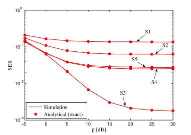
Figure 2: Analytical and simulated SER values for a MRC receiver with BPSK modulation in flat Rayleigh fading for scenarios S1-S5 with parameters: $n_{R}=3$ and $\varsigma=1$.

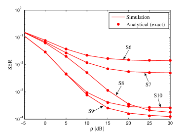
Figure 3: Analytical and simulated SER values for a MRC receiver with BPSK modulation in flat Rayleigh fading for scenarios S6-S10 with parameters: $n_{R}=3$ and $\varsigma=10$.

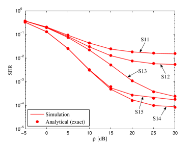
Figure 4: Analytical and simulated SER values for a MRC receiver with QPSK modulation in flat Rayleigh fading for scenarios S11-S15 with parameters: $n_{R}=3$ and $\varsigma=30$.

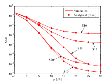
Figure 5: Analytical and simulated SER values for a MRC receiver with QPSK modulation in flat Rayleigh fading for scenarios S16-S20 with parameters: $n_{R}=6$ and $\varsigma=20$.

Figures 2 and 3 verify the analytical results in (32) for BPSK modulation with simulations and also explore the effect of different power profiles. In Fig. 2, a low SIR is considered with $\varsigma=1$. Here, S1 is the worst case since the desired signal profile is aligned with the interferer and the profile is rapidly decaying giving little diversity. S3 is the best since the profiles are opposing and the best desired signal aligns with the weakest interference. Since Fig. 2 has a low SIR the major impact on performance is caused by the presence or absence of a high SIR or low SIR at each antenna. In Fig. 3, the same power profiles are considered but at higher SIR, $\varsigma=10$, the order is changed. S6 is still the worst as this scenario has high interference at all antennas and little diversity. In contrast S8 is no longer the best with S9 now giving better performance. Note that S9 has greater diversity with an even spread of power across the antennas and this becomes more important at high SIR.
Another comparison between scenarios can be seen in Table I. Note that in Fig. 2 the ordering based on $m_{P}$ correctly identifies the best and worst scenarios whereas in Fig. 3 the $m_{p}$ metric suggest that S8 is best whereas S9 is better. The $m_{p}$ metric gives some intuition about macrodiversity MRC performance, especially at low SIR, but it doesn’t accurately capture diversity effects (seen in the lower tail of the combiner output) which are needed for accurate performance prediction.
In Fig. 4, the same power profiles are considered for QPSK transmission. Here, the exact results from Sec. III-B are verified by simulation. In particular, the SER expression in (43) for QPSK modulation is used along with (32) and (46). The relative performance provided by the 5 scenarios is the same as in Fig. 3 except that the cross over of S13 and S15 in Fig. 4 (equivalent to the cross over of S8 and S10 in Fig. 3) does not occur until $\mbox{SNR}>30$ dB.
Finally, in Fig. 5 we consider the six antenna receiver where antennas 1,2 are co-located, antennas 3,4 are co-located elsewhere and antennas 5,6 are also co-located and separated from antennas 1-4. Here, the long term receive SNR of a source at antennas 1 and 2 will be the same. Hence, we use the perturbation approach of Sec. III-D to obtain results. Fig. 5 validates the perturbation approach by simulation and shows a large performance improvement relative to Fig. 4 due to the increased number of antennas. Again, the results due to the five scenarios follow the same order as in Figs. 3 and 4. Note that when $\alpha=1$ for both desired and interfering sources, the system layout is microdiversity. Hence, scenarios S4, S9, S14 and S19 provide microdiversity results.

V Conclusion

Exact SER results are derived for BPSK and $M$-QAM modulations in a Rayleigh fading macrodiversity system employing MRC. The results have applications to several systems of current interest in communications including network MIMO and cooperative communications. The analysis is used to study the effects of the macrodiversity power profiles on MRC performance. It is shown that simple power metrics may capture several features of MRC performance but the impact of diversity in a distributed system is important at realistic SINR values. Here, the exact results are necessary to provide an accurate performance measure. In general, performance improves as the desired signal dominates the interferer at some antennas and as the desired power is spread more evenly over the receive antennas. The exact balance between these two key features is difficult to obtain in a simple form but is provided by the exact solutions given.

Appendix A Calculation of the cdf of $\gamma$

Since each term in the summation of (17) depends on the algebraic sign of $\beta_{ik}$, the final cdf has two parts as below

$$F_{\gamma}\left(r\right) =\sum_{i=1}^{n_{R}}\sum_{k\neq i}^{n_{R}}F_{ik}\left(r\right),$$ (56)

where $F_{ik}\left(r\right)=F_{ik}^{1}\left(r\right)$ for $\beta_{ik}>0$ and $F_{ik}\left(r\right)=F_{ik}^{2}\left(r\right)$ for $\beta_{ik}<0$. In subsection A-A we derive $F_{ik}^{1}\left(r\right)$ followed by the derivation of $F_{ik}^{2}\left(r\right)$ in subsection A-B.

A-A Derivation of $F_{ik}^{1}\left(r\right)$

From the joint pdf in (17), when $\beta_{ik}>0$, $F_{ik}^{1}\left(r\right)$ is given by

$$F_{ik}^{1}\left(r\right) =\iint_{\mathcal{F}_{1}}f_{X,Y}\left(x,y\right)dxdy,$$ (57)

where $\mathcal{F}_{1}=\left\{x,y:x,y\geq 0,y-\frac{Q_{i}}{P_{i1}}x\geq 0,y-\frac{x^{2}}{r}\geq 0\right\}$. By using standard methods for 2-D integrals we arrive at

$$F_{ik}^{1}\left(r\right) =\frac{P_{i1}\xi_{ik}}{\beta_{ik}}-\xi_{ik}\int_{\frac{rQ_{i}}{P_{i1}}}^{\infty}\int_{\frac{xQ_{i}}{P_{i1}}}^{\frac{x^{2}}{r}}e^{-\frac{x}{P_{i1}}}e^{-\beta_{ik}\left(y-\frac{Q_{i}x}{P_{i1}}\right)}dydx.$$ (58)

The final result then becomes

$$\begin{split}F_{ik}^{1}\left(r\right)&=\frac{P_{i1}\xi_{ik}}{\beta_{ik}}\left(1-e^{-\frac{rQ_{i}}{P_{i1}^{2}}}\right)+\frac{\xi_{ik}}{2\beta_{ik}}\sqrt{\frac{\pi r}{\beta_{ik}}}e^{\frac{r\omega_{ik}^{2}}{4\beta_{ik}}}\\ &\qquad\qquad\qquad\qquad\times\left(1-\Phi\left(\sqrt{r\beta_{ik}}\alpha_{ik}\right)\right),\end{split}$$ (59)

where

$$\omega_{ik} =\frac{1-\beta_{ik}Q_{i}}{P_{i1}},$$ (60a)

$$\alpha_{ik} =\frac{Q_{i}}{P_{i1}}+\frac{\omega_{ik}}{2\beta_{ik}}.$$ (60b)

The expression in (28) follows using standard methods of integration in (58) and employing the following integral identity [17] where necessary:

$$\int_{\alpha}^{\infty}e^{-\beta x^{2}}dx =\frac{1}{2}\sqrt{\frac{\pi}{\beta}}\left(1-\Phi\left(\sqrt{\beta}\alpha\right)\right).$$ (61)

A-B Derivation of $F_{ik}^{2}\left(r\right)$

From the joint pdf in (17), when $\beta_{ik}<0$, $F_{ik}^{2}\left(r\right)$ is given by

$$F_{ik}^{2}\left(r\right) =\iint_{\mathcal{F}_{2}}f_{X,Y}\left(x,y\right)dxdy,$$ (62)

where $\mathcal{F}_{2}=\left\{x,y:x,y\geq 0,y-\frac{Q_{i}}{P_{i1}}x\leq 0,y-\frac{x^{2}}{r}\geq 0\right\}$. By using standard methods for 2-D integrals we arrive at

$$F_{ik}^{2}\left(r\right) =-\xi_{ik}\int_{0}^{\frac{rQ_{i}}{P_{i1}}}\int_{\frac{x^{2}}{r}}^{\frac{xQ_{i}}{P_{i1}}}e^{-\frac{x}{P_{i1}}}e^{-\beta_{ik}\left(y-\frac{Q_{i}x}{P_{i1}}\right)}dydx.$$ (63)

The final result then becomes

$$\begin{split}F_{ik}^{2}\left(r\right)&=\frac{P_{i1}\xi_{ik}}{\beta_{ik}}\left(1-e^{-\frac{rQ_{i}}{P_{i1}^{2}}}\right)-\frac{\xi_{ik}}{2\beta_{ik}}\sqrt{\frac{\pi r}{-\beta_{ik}}}e^{\frac{r\omega_{ik}^{2}}{4\beta_{ik}}}\\ &\times\left(\mbox{erfi}\left(\sqrt{-r\beta_{ik}}\alpha_{ik}\right)+\mbox{erfi}\left(\frac{1}{2}\sqrt{\frac{r}{-\beta_{ik}}}\omega_{ik}\right)\!\right),\end{split}$$ (64)

where

$$\mbox{erfi}\left(x\right) =\frac{\Phi\left(jx\right)}{j}.$$ (65)

The function $\mbox{erfi}\left(.\right)$ is the error function with a complex argument defined in [17]. Note that the square roots appearing in (29) are the positive square root of $\beta_{ik}$. The expression in (29) follows using standard methods of integration and employing the following integral identity [17] where necessary:

$$\int e^{ax^{2}}dx =\frac{1}{2}\sqrt{\frac{\pi}{a}}\mbox{erfi}\left(\sqrt{a}x\right).$$ (66)

Appendix B Derivation of the exact SER

The integral in (45) is required for the exact SER analysis. Substituting $F_{\gamma}\left(w^{2}/b\right)$ from (27) into (45) gives two new integrals involving $F^{1}_{ik}\left(w^{2}/b\right)$ or $F^{2}_{ik}\left(w^{2}/b\right)$, which are given in (28) and (29). These two integrals can be written in terms of known functions and two fundamental probability integrals that we denote $I_{1}\left(\alpha,\beta\right)$ and $I_{2}\left(\alpha,\beta\right)$. These integrals are computed below.

B-A Integral Form I

Consider the integral,

$$I_{1}\left(\alpha,\beta\right) =\int_{0}^{\infty}xe^{-\beta x^{2}}Q\left(x\right)\Phi\left(j\alpha x\right)dx.$$ (67)

Applying the integral forms of $Q(.)$ and $\Phi(.)$ gives

$$I_{1}\left(\alpha,\beta\right) =\frac{2j}{\pi}\int_{0}^{\infty}\int_{\frac{x}{\sqrt{2}}}^{\infty}\int_{0}^{\alpha x}xe^{-\beta x^{2}-t_{1}^{2}+t_{2}^{2}}dt_{2}dt_{1}dx.$$ (68)

Using the substitutions, $t_{1}=r\cos\theta$ and $t_{2}=r\sin\theta$, the integral then becomes

$$I_{1}\left(\alpha,\beta\right) =\frac{2j}{\pi}\int_{0}^{\infty}\int_{0}^{\phi}\int_{r_{1}}^{r_{2}}xre^{-\beta x^{2}-r^{2}cos\left.2\theta\right.}drd\theta dx,$$ (69)

where $\tan\phi=\alpha\sqrt{2}$, $r_{1}=x/\sqrt{2}\cos\theta$ and $r_{2}=\alpha x/\sin\theta$. Using standard methods of integration with some simplifications we obtain

$$\begin{split}I_{1}\left(\alpha,\beta\right)&=\frac{j}{2\pi\beta}\int_{0}^{\alpha\sqrt{2}}\frac{dt}{t^{2}-1-2\beta}\\ &\qquad\qquad-\frac{j\alpha^{2}}{2\pi\beta}\int_{0}^{\alpha\sqrt{2}}\frac{dt}{\left(\alpha^{2}-\beta\right)t^{2}-\alpha^{2}}.\end{split}$$ (70)

Defining

$$I_{11}\left(\alpha,\beta\right) =\int_{0}^{\alpha\sqrt{2}}\frac{dt}{t^{2}-1-2\beta},$$ (71)

$$I_{12}\left(\alpha,\beta\right) =\int_{0}^{\alpha\sqrt{2}}\frac{dt}{\left(\alpha^{2}-\beta\right)t^{2}-\alpha^{2}},$$ (72)

allows (70) to be rewritten as

$$I_{1}\left(\alpha,\beta\right) =\frac{j}{2\pi\beta}I_{11}\left(\alpha,\beta\right)-\frac{j\alpha^{2}}{2\pi\beta}I_{12}\left(\alpha,\beta\right).$$ (73)

The integral in (71) and (72) can be solved in closed form to give

$$I_{11}\left(\alpha,\beta\right) =-\frac{1}{\sqrt{2\beta+1}}\tanh^{-1}\left(\frac{\alpha\sqrt{2}}{\sqrt{2\beta+1}}\right)$$ (74)

and

$$\!\!\!I_{12}\left(\alpha,\beta\right)\!\! =\!\!\begin{cases}-\frac{\sqrt{2}}{\alpha}&\quad\beta=\alpha^{2}\\ -\frac{1}{\alpha\sqrt{\beta-\alpha^{2}}}\tan^{-1}\!\!\left(\sqrt{2\left(\beta-\alpha^{2}\right)}\right)&\quad\mbox{otherwise}.\end{cases}$$ (75)

Note that some intermediate steps in the derivation show that $1+2\beta>2\alpha^{2}$ is required for the existence of (67). This constraint is satisfied by the current problem. This can easily be seen by substituting the arguments of both $I_{1}\left(.,.\right)$ functions in (48) in to $1+2\beta>2\alpha^{2}$ followed by simplifications using (30).

B-B Integral Form II

Consider the integral,

$$I_{2}\left(\alpha,\beta\right)=\int_{0}^{\infty}xe^{\beta x^{2}}Q\left(x\right)\left(1-\Phi\left(\alpha x\right)\right)dx.$$ (76)

Applying the integral forms of $Q(.)$ and $\Phi(.)$ we obtain

$$I_{2}\left(\alpha,\beta\right) =\frac{2}{\pi}\int_{0}^{\infty}\int_{\frac{x}{\sqrt{2}}}^{\infty}\int_{\alpha x}^{\infty}xe^{\beta x^{2}-t_{1}^{2}-t_{2}^{2}}dt_{2}dt_{1}dx.$$ (77)

Following the same procedure as in Appendix B-A and with some simplifications we arrive at

$$\begin{split}I_{2}\left(\alpha,\beta\right)=\frac{\alpha^{2}}{2\pi\beta}&\int_{0}^{\phi}\frac{d\theta}{\alpha^{2}-\beta\sin^{2}\theta}\\ &+\frac{1}{2\pi\beta}\int_{\phi}^{\pi/2}\frac{d\theta}{1-2\beta\cos^{2}\theta}-\frac{1}{4\beta},\end{split}$$ (78)

where $\tan\phi=\sqrt{2}\alpha$. Making another substitution as $t=\tan\theta$ in (78) gives

$$\begin{split}I_{2}\left(\alpha,\beta\right)=\frac{\alpha^{2}}{2\pi\beta}&\int_{0}^{\sqrt{2}\alpha}\frac{dt}{\left(\alpha^{2}-\beta\right)t^{2}+\alpha^{2}}\\ &+\frac{1}{2\pi\beta}\int_{\sqrt{2}\alpha}^{\infty}\frac{dt}{t^{2}+1-2\beta}-\frac{1}{4\beta}.\end{split}$$ (79)

Defining

$$I_{21}\left(\alpha,\beta\right) =\int_{0}^{\sqrt{2}\alpha}\frac{dt}{\left(\alpha^{2}-\beta\right)t^{2}+\alpha^{2}},$$ (80)

$$I_{22}\left(\alpha,\beta\right) =\int_{\sqrt{2}\alpha}^{\infty}\frac{dt}{t^{2}+1-2\beta},$$ (81)

allows (79) to be rewritten as

$$I_{2}\left(\alpha,\beta\right) =\frac{\alpha^{2}}{2\pi\beta}I_{21}\left(\alpha,\beta\right)+\frac{1}{2\pi\beta}I_{22}\left(\alpha,\beta\right)-\frac{1}{4\beta}.$$ (82)

The integrals in (80) and (81) can be solved in closed form to give

$$\!\!\!I_{21}\left(\alpha,\beta\right)\!\! =\!\!\begin{cases}\frac{\sqrt{2}}{\alpha}&\quad\alpha^{2}\!=\!\beta\\ \frac{1}{\alpha\sqrt{\alpha^{2}-\beta}}\tan^{-1}\!\left(\!\sqrt{2\left(\alpha^{2}\!-\!\beta\right)}\right)&\quad\mbox{otherwise}\end{cases}$$ (83)

and

$$\!\!\!I_{22}\left(\alpha,\beta\right) =\begin{cases}\frac{1}{\sqrt{2}\alpha}&\quad 1=2\beta\\ \frac{1}{\sqrt{2\beta-1}}\coth^{-1}\left(\frac{\sqrt{2}\alpha}{\sqrt{\left.2\beta-1\right.}}\right)&\quad\mbox{otherwise}.\end{cases}$$ (84)

As for $I_{1}\left(\alpha,\beta\right)$ there is an associated region of validity, $1+2\alpha^{2}>2\beta$, which is satisfied by the problem.

Dushyantha Basnayaka (S’11-M’12) was born in 1982 in Colombo, Sri Lanka. He received the B.Sc.Eng degree with 1st class honors from the University of Peradeniya, Sri Lanka, in Jan 2006. He is currently working towards for his PhD degree in Electrical and Computer Engineering at the University of Canterbury, Christchurch, New Zealand. He was an instructor in the Department of Electrical and Electronics Engineering at the University of Peradeniya from Jan 2006 to May 2006. He was a system engineer at MillenniumIT (a member company of London Stock Exchange group) from May 2006 to Jun. 2009. Since Jul. 2009 he is with the communication research group at the University of Canterbury, New Zealand. D. A. Basnayaka is a recipient of University of Canterbury International Doctoral Scholarship for his doctoral studies at UC. His current research interest includes all the areas of digital communication, especially macrodiversity wireless systems. He holds one pending US patent as a result of his doctoral studies at UC.

Peter Smith (M’93-SM’01) received the B.Sc degree in Mathematics and the Ph.D degree in Statistics from the University of London, London, U.K., in 1983 and 1988, respectively. From 1983 to 1986 he was with the Telecommunications Laboratories at GEC Hirst Research Centre. From 1988 to 2001 he was a lecturer in statistics at Victoria University, Wellington, New Zealand. Since 2001 he has been a Senior Lecturer and Associate Professor in Electrical and Computer Engineering at the University of Canterbury in New Zealand. Currently, he is a full Professor at the same department. His research interests include the statistical aspects of design, modeling and analysis for communication systems, especially antenna arrays, MIMO, cognitive radio and relays.

Philippa Martin (S 95-M 01-SM 06) received the B.E. (Hons. 1) and Ph.D. degrees in electrical and electronic engineering from the University of Canterbury, Christchurch, New Zealand, in 1997 and 2001, respectively. From 2001 to 2004, she was a postdoctoral fellow, funded in part by the New Zealand Foundation for Research, Science and Technology (FRST), in the Department of Electrical and Computer Engineering at the University of Canterbury. In 2002, she spent 5 months as a visiting researcher in the Department of Electrical Engineering at the University of Hawaii at Manoa, Honolulu, Hawaii, USA. Since 2004 she has been working at the University of Canterbury as a lecturer and then as a senior lecturer. Currently, she is an Associate Professor at the same department. In 2007, she was awarded the University of Canterbury, College of Engineering young researcher award. She served as an Editor for the IEEE Transactions on Wireless Communications 2005-2008 and regularly serves on technical program committees for IEEE conferences. Her current research interests include multilevel coding, error correction coding, iterative decoding and equalization, space-time coding and detection, cognitive radio and cooperative communications in particular for wireless communications

References

• [1] M.Β K. Simon and M.Β S. Alouini, Digital Communications over Fading Channels: A Unified Approach to Performance Analysis, New York, NY, USA: Wiley, 2000.
• [2] Q. H. Ngo, E. G. Larsson and T. L. Marzetta, β€œUplink power efficiency of multiuser MIMO with very large antenna arrays,” Proc. Allerton Conf. on Communication, Control, and computing, Illinois, USA, pp. 1272–1279, 2011.
• [3] J. Zhu, Qiang Li and Qinghua Li, β€œPragmatic adaptive MRC and MMSE MIMO-OFDM receiver algorithum,” U.S. Patent 20080310486, Dec. 18, 2008.
• [4] D. R. Pauluzzi and N. C. Beaulieu, β€œA Comparison of SNR Estimation Techniques for the AWGN Channel,” IEEE Trans. Commun., vol.Β 48, No. 10, pp. 1681–1691, Oct. 2000.
• [5] J. Cui and A. U. H. Sheikh, β€œOutage probability of cellular radio systems using maximal ratio combining in the presence of multiple interferers,” IEEE Trans. Commun., vol.Β 47, No. 47, pp. 1121–1124, Aug. 1999.
• [6] Y. Tokgoz and B. D. Rao, β€œThe effect of imperfect channel estimation on the performance of maximum ratio combining in the presence of cochannel interference,” IEEE Trans. Veh. Technol., vol. 55, no. 5, pp. 1527–1534, Sep. 2006.
• [7] E. Biglieri, R. Calderbank, A. Constantinides, A. Goldsmith, A. Paulraj and H. V. Poor, MIMO Wireless Communication, 1stΒ ed, Cambridge: Cambridge University Press, 2007.
• [8] S. Catreux, R. L. Kirlin and P. F. Driessen, β€œCapacity and performance of multiple-input multiple-output wireless systems in a cellular context,” IEEE PACRIM, Victoria, BC, Canada, pp. 516–519, 1999.
• [9] J. Zhang, X. Bi and Y. Wang, β€œAntenna pairing for space-frequency block codes in edge-excited distributed antenna systems” IEEE PIMRC, Istanbul, Turkey, pp. 117–122, 2010.
• [10] S. Venkatesan, A. Lozano and R. Valenzuela, β€œNetwork MIMO: Overcoming intercell interference in indoor wireless systems,” IEEE ACSSC, pp. 83–87, Jul. 2007.
• [11] M. K. Karakayali, G. J. Foschini, and R. A. Valenzuela, β€œNetwork coordination for spectrally efficient communications in cellular systems,” IEEE Trans. on Wireless Commun. Mag., vol. 13, no. 4, pp. 56–61, Aug. 2006.
• [12] M. Matthaiou, N. D. Chatzidiamantis, G. K. Karagiannidis, and J. A. Nossek, β€œOn the capacity of generalized-K fading MIMO channels,” IEEE Trans. Signal Processing, vol. 58, no. 11, pp. 5939 -5944, November 2010.
• [13] C. Zhong, K.-K. Wong, and S. Jin, β€œCapacity bounds for MIMO Nakagami-m fading channels,” IEEE Trans. Signal Processing, vol. 57, no. 9, pp. 3613 -3623, Sept. 2009.
• [14] J. G. Proakis, Digital Communications, 4thΒ ed, New York: McGraw-Hill, 2001.
• [15] A. Prudnikov, Y. Brychkov and O. Marichev, β€œTables and Integrals,” 2ndΒ ed, Gordon and Breach, New York, 1986.
• [16] D. Lee, B. Clerckx, E. Hardouin, D. Mazzarese, S. Nagata, and K. Sayana, β€œCoordinated multipoint transmission and reception in LTE-Advanced: Deployment scenarios and operational challenges,” IEEE Commun. Mag., vol. 50, no. 2, pp. 148–155, 2012.
• [17] I. S. Gradshteyn and I. M. Ryzhik, Table of Integrals, Series, and Products, 7thΒ ed, Boston: Academic Press, 2000.
• [18] A. Goldsmith, Wireless Communication, 4thΒ ed, New York: McGraw-Hill, 2000.
• [19] P. J. Smith, β€œExact performance analysis of optimum combining with multiple interferers in flat Rayleigh fading,” IEEE Trans. Commun., vol. 55, no. 9, pp. 1674–1677, Sep. 2007.
• [20] K. S. Miller, Multidimensional Gaussian Distributions, 1stΒ ed, New York: John Wiley & Sons, 1964.
• [21] A. Firag, P. J. Smith, H. Suraweera and A. Nallanathan, β€œBeamforming in correlated MISO systems with channel estimation error and feedback delay,” IEEE Trans. on Wireless Commun., vol. 10, no. 8, pp. 2592–2602, 2011.
• [22] O. Lieberman, β€œA Laplace approximation to the moments of a ratio of quadratic forms,” Biometrika, vol. 81, no. 4, pp. 681–690, Dec 1994.
• [23] H. Gao, P. J. Smith and M. V. Clark, β€œTheoretical reliability of MMSE linear diversity combining in Rayleigh-fading additive interference channels,” IEEE Trans. Commun., vol.Β 46, no. 5, pp. 666–672, May. 1998.