Concentration Dependence of Rheological Properties of Telechelic Associative Polymer Solutions

Abstract

We consider concentration dependence of rheological properties of associative telechelic polymer solutions. Experimental results for model telechelic polymer solutions show rather strong concentration dependence of rheological properties. For solutions with relatively high concentrations, linear viscoelasticity deviates from the single Maxwell behavior. The concentration dependence of characteristic relaxation time and moduli is different in high and low concentration cases. These results suggest that there are two different concentration regimes. We expect that densely connected (well percolated) networks are formed in high-concentration solutions, whereas sparsely connected (weakly percolated) networks are formed in low-concentration solutions. We propose single chain type transient network models to explain experimental results. Our models incorporate the spatial correlation effect of micellar cores and average number of elastically active chains per micellar core (the network functionality). Our models can reproduce non-single Maxwellian relaxation and nonlinear rheological behavior such as the shear thickening and thinning. They are qualitatively consistent with experimental results. In our models, the linear rheological behavior is mainly attributable to the difference of network structures (functionalities). The nonlinear rheological behavior is attributable to the nonlinear flow rate dependence of the spatial correlation of micellar core positions.

I Introduction

Telechelic associative polymers which have hydrophilic main chains and hydrophobic chain ends form self-assembled micellar structures in aqueous solutionsLarson (1999); Annable et al. (1993); Tripathi et al. (2006). If the concentration of telechelic polymers is sufficiently high, the micellar cores are bridged by polymers to form a percolated, network like structure. Such a network structure shows various kinds of interesting rheological behavior and rheological properties of telechelic associative polymer solutions have been extensively studied. For example, various experimental results have been reported for hydrophobically modified ethoxylated urethane (HEUR) aqueous solutions Annable et al. (1993); Xu et al. (1996); Tam et al. (1998); Tripathi et al. (2006).

One characteristic rheological property of telechelic polymer solutions is the linear viscoelasticity being well described by a single Maxwellian form in a rather wide range of experimental parameters. Theoretically, such a rheological property can be explained in the framework of the transient network modelGreen and Tobolsky (1946); Tanaka and Edwards (1992). The characteristic relaxation time is considered to be the dissociation time of a chain end, and the characteristic modulus is considered to be the elastic modulus of the network formed by telechelic polymers. However, the simple description by the transient network model is not always valid. For relatively high concentration solutions, deviation from the single Maxwellian form has been reportedCathébras et al. (1998); Séréro et al. (1998, 2000). In most of the transient network type models, such non-single Maxwellian relaxation cannot be explained straightforwardly. (This is due to the nature of the mean field type approximations in the transient network type models.) This implies that we need to incorporate some additional factors, which are affected by the polymer concentration, to the models.

Another characteristic rheological property is that telechelic polymer solutions often exhibit shear thickening behavior. The transient network model has been improved to reproduce such experimentally observed nonlinear rheological behavior. In some improved versions of the transient network modelWang (1992); Marrucci et al. (1993); Vaccaro and Marrucci (2000); Indei et al. (2005); Indei (2007a, b); Koga and Tanaka (2010); Tripathi et al. (2006), the nonlinear elasticity (or finite extensively) and the stretch dependent dissociation rate are introduced. It has been reported that the combination of the nonlinear elasticity and the stretch dependent dissociation rate can reproduce several nonlinear rheological properties. For example, models by Tripathi et al.Tripathi et al. (2006) and by Indei, Koga and TanakaIndei et al. (2005); Indei (2007a, b); Koga and Tanaka (2010) can reproduce several nonlinear features such as the shear thickening and thinning, by tuning some fitting parameters (which represent the strengths of the nonlinear elasticity and the stretch dependent dissociation).

However, a recent study showed that conventionally proposed transient network models cannot explain some rheological data of a HEUR aqueous solutionSuzuki et al. (2012), such as the first normal stress coefficient ($\Psi_{1}$) data that exhibit no nonlinearity in the shear-thickening regime of the shear viscosity ($\eta$). To explain this experimental fact, a new transient network model with an anisotropic (and shear rate dependent) bridge formation process was proposed. The anisotropic bridge formation model can qualitatively explain this behavior of $\Psi_{1}$ as well as the shear thickening (and thinning) behavior of $\eta$ under fast shear, the latter being explained also by conventionally proposed models. Although the new model provides a new viewpoint to understand dynamical behavior of telechelic polymer solutions, it was constructed in a phenomenological way and the molecular level mechanism of anisotropic bridge formation has not been specified explicitly.

From the viewpoint of nonequilibrium dynamics of flowing systems, anisotropies under flow are physically reasonable. For example, colloid dispersions show structural anisotropies and nonlinear rheological behavior under flowVerduin et al. (1996); Brader (2010). The interaction potential and spatial correlation between colloid particles are important to understand/analyze such systems. In telechelic polymer solutions, there are also interactions and spatial correlations between micellar coresSemenov et al. (1995); Khalatur and Khokhlov (1996); Séréro et al. (1998, 2000) (although their forms are quite different from colloid dispersions). Clearly, such interactions or spatial correlations depend on the polymer concentration, and thus we expect the rheological properties of telechelic polymer solutions to be rather strongly dependent on the concentration. Indeed, we can find rather strong concentration dependence of several rheological properties in literatureAnnable et al. (1993); Xu et al. (1996).

This implies that we should design a model for telechelic polymer solutions which directly takes into account the spatial correlation (or the interaction potential) of the micellar cores, to naturally reproduce concentration dependence of rheological properties and anisotropic correlations and nonlinear rheological behavior under shear. Nevertheless, the importance of the spatial correlations for the rheology of telechelic polymer solutions has been rarely pointed out. Especially, the spatial correlations have been overlooked or ignored for single chain type models, as far as the authors know.

In this work, we conducted linear viscoelastic measurements for HEUR aqueous solutions with different concentrations. We show that the linear rheological behavior is strongly affected by the concentration. The experimental data suggest that there are two different concentration regimes. Then we propose a simple but non-trivial single chain type transient network models for telechelic associative polymers, which explicitly take into account the spatial correlation information. We show that our models give both single and non-single Maxwellian relaxation moduli depending on the polymer concentration. We also show that nonlinear rheological behavior such as the shear thickening and thinning can be reproduced by our models considering neither nonlinear elasticity nor stretch dependence of the bridge reconstruction rates. We discuss concentration dependence of rheological data from the view point of the transient network type models.

II Experimental

II.1 Materials and Measurements

HEUR with hexadecyl end groups and polyethylene oxide (PEO) main chain was used. The HEUR was synthesized previouslySuzuki et al. (2012) with a conventional method, and the molecular weight and polydispersity index were $M_{w}=4.6\times 10^{4}$ and $M_{w}/M_{n}=1.35$ (the PEO precursor molecular weight and polydispersity index were $M_{w}=1.9\times 10^{4}$ and $M_{w}/M_{n}=1.1$). The details of the synthesis and characteristics are found in Ref. Suzuki et al. (2012).

The HEUR aqueous solutions were prepared by dissolving HEUR into distilled water through stirring for $24\text{ hours}$. For comparison, the PEO aqueous solutions with a similar molecular weight and the same concentrations as the HEUR solutions were also prepared. The PEO sample was purchased from Aldrich ($M_{w}=3.9\times 10^{4}$, $M_{w}/M_{n}=1.08$) and dissolved into distilled water.

Storage and loss moduli, $G^{\prime}(\omega)$ and $G^{\prime\prime}(\omega)$, were measured for HEUR aqueous solutions at various temperatures and concentrations. The measurements were conducted with a stress-controlled rheometer (MCR-301, Anton Paar). A cone-plate type fixture with the diameter $d=75\text{ mm}$ and the cone angle $\theta=1^{\circ}$ was utilized. The measurement temperatures were $T=5,10,15,20,$ and $25^{\circ}\text{C}$, and the concentration $c$ was varied from $1\text{wt\%}$ to $10\text{wt\%}$. The angular frequency range was set as $0.03$ rad/s $\leq\omega\leq$ $500$ rad/s. Storage and loss moduli of PEO aqueous solutions with the same concentrations and the similar molecular weight as HEUR solutions were also measured in the same condition. (Due to the low moduli of solutions and the limitation of the equipment, only the loss moduli data in a limited range $1\text{ rad/s}\lesssim\omega\lesssim 10\text{ rad/s}$ were obtained with acceptable accuracy.)

II.2 Results

First we show the master curves for the storage and loss moduli, $G^{\prime}(\omega)$ and $G^{\prime\prime}(\omega)$ of $1\text{wt\%}$ HEUR aqueous solution at the reference temperature $T_{r}=25^{\circ}\text{C}$ in Figure 1. The master curves (master plots of $b_{T,0}^{-1}G^{\prime}$ and $b_{T,0}^{-1}G^{\prime\prime}$ against $a_{T,0}\omega$) are constructed by shifting $G^{\prime}(\omega)$ and $G^{\prime\prime}(\omega)$ data at different temperatures horizontally and vertically, to superimpose the low frequency data. The horizontal and vertical shirt factors are denoted by $a_{T,0}$ and $b_{T,0}$, respectively. As reported in the previous workSuzuki et al. (2012), the time-temperature superposition works well for this HEUR solution and the $G^{\prime}(\omega)$ and $G^{\prime\prime}(\omega)$ data are fitted well by a single Maxwell model, except the high frequency region.

$$G^{\prime}(\omega)=G_{0}\frac{(\tau\omega)^{2}}{1+(\tau\omega)^{2}},\qquad G^{\prime\prime}(\omega)=G_{0}\frac{\tau\omega}{1+(\tau\omega)^{2}}$$ (1)

Here $\tau$ and $G_{0}$ are the characteristic relaxation time and modulus, respectively. The deviation in the high frequency region means that there is another relaxation mode of which temperature dependence is different from the relaxation mode in the low frequency region. In the followings, we call these modes in the high and low frequency regions as fast and slow modes, respectively.

Ng et al.Ng et al. (2000) proposed that the fast mode is due to the relaxation of micellar cores, whereas Bedrov et al.Bedrov et al. (2002) claimed that the fast mode corresponds to the local relaxation of hydrophilic main chains. If the fast mode corresponds to the local relaxation mode of PEO chains, it should show the same temperature dependence as a PEO aqueous solution without associative end groups. We determined the horizontal shift factor $a_{T,1}$ of the $1\text{wt\%}$ PEO solution (utilizing the vertical shift factor $b_{T,1}=T/T_{r}$). Then we shifted the $G^{\prime}$ and $G^{\prime\prime}$ data of the $1\text{wt\%}$ HEUR solution with the shift factors $a_{T,1}$ and $b_{T,1}$. The result is shown in Figure 2, and $a_{T,1}$ is compared with $a_{T,0}$ of the HEUR solution in Figure 3. As shown in Figure 2, $a_{T,1}$ allows the $G^{\prime}(\omega)$ and $G^{\prime\prime}(\omega)$ data to collapse into master curves at high frequencies where the fast mode is observed. $a_{T,1}$ is less dependent on $T$ compared with $a_{T,0}$. This result means that the fast mode corresponds to the local relaxation of PEO chains, as claimed by Bedrov et al.Bedrov et al. (2002). However, it should be also noticed that the relaxation time and the characteristic modulus of the fast mode of the HEUR solution are much larger than those of the PEO solution with the same concentration, mostly because the HEUR chains form an associated network-like structure and the relaxation modes of such a network are different from ones of the free chains. We will discuss this point later. Although we have shown the master curves only for the $1\text{wt\%}$ solution case, we can similarly construct master curves for slow and fast modes for other concentration cases.

We show the storage and loss moduli data at $T=25^{\circ}\text{C}$ for different concentrations ($c=1,2,5,$ and $10\text{wt\%}$) in Figure 4. We can observe slow and fast modes for all concentrations. However, the $\omega$ dependence of $G^{\prime}(\omega)$ and $G^{\prime\prime}(\omega)$ changes with the concentration rather largely. This change is more prominent for the fast mode than for the slow mode. For $c=1$ and $2\text{wt\%}$, the $G^{\prime\prime}(\omega)$ at high $\omega$ (the fast mode) is almost proportional to $\omega$, which indicates that the fast and slow modes are rather separated. For $c=5$ and $10\text{wt\%}$, on the other hand, the $G^{\prime\prime}(\omega)$ at high $\omega$ becomes less dependent on $\omega$, and the fast and slow modes are not well separated compared with the cases of the $1$ and $2\text{wt\%}$ solutions. The slow mode distribution also changes with the concentration, although it is not so clear in Figure 4. To see this change clearly, we show the $G^{\prime}(\omega)$ and $G^{\prime\prime}(\omega)$ rescaled by the characteristic time $\tau$ and modulus $G_{0}$ for the slow mode in Figure 5. It is evident from Figure 5 that the slow mode deviates from the single Maxwellian form as the concentration increases. Similar non-single Maxwellian relaxation moduli have already been reported in some experimental or simulation studiesCathébras et al. (1998); Séréro et al. (1998, 2000); Tae et al. (2002); Berret et al. (2003); Castelletto et al. (2004); Cass et al. (2008); Sprakel et al. (2009). For example, Berret and coworkers Cathébras et al. (1998); Séréro et al. (1998, 2000) reported that the shear relaxation moduli of solutions of F-HEUR (HEUR with perfluoroalkyl chain ends) can be fitted by the stretched exponential form, $G(t)=G_{0}\exp[-(t/\tau)^{\alpha}]$ (with $G_{0}$, $\tau$ and $\alpha$ being the characteristic modulus, characteristic relaxation time, and the power-law exponent). Mistry et al. reported non-single Maxwell relaxation modulus data for relatively high concentration poly(butylene oxide)-(etylene oxide)-(butylene oxide) triblock copolymer solutionsMistry et al. (2006). Some shear relaxation modulus data for relatively high concentration HEUR solutionsAnnable et al. (1993); Xu et al. (1996) also deviate from the single Maxwellian form.

Finally we show the characteristic relaxation time $\tau$ and modulus $G_{0}$ data of the slow mode in Figure 6. Both $\tau$ and $G_{0}$ depend on the HEUR concentration. The concentration dependence at low and high concentration regions can be individually fitted to power laws. The characteristic time $\tau$ depends on the concentration $c$ as $\tau\propto c^{0.63}$ and $\tau\propto c^{0.32}$ for low and high concentration regions, respectively (Figure 6(a)). Similarly, the characteristic modulus depends on $c$ as $G_{0}\propto c^{2.3}$ and $G_{0}\propto c^{1.8}$ (Figure 6(b)). Both $\tau$ and $G_{0}$ data show stronger $c$-dependence at the low concentration region. From Figure 6, the crossover concentration $c_{c}$ is roughly estimated as $c_{c}\approx 4\text{wt\%}$. At $c>c_{c}$, the $G^{\prime}(\omega)$ and $G^{\prime\prime}(\omega)$ data deviate considerably from the single Maxwellian forms, as noted in Figure 5. Here it should be noted that Annable et al.Annable et al. (1993) already measured the concentration dependence of $\tau$ and $G_{0}$ of HEUR solutions systematically, and reported similar data. (They proposed a statistical model to explain their experimental data. Their model takes account of superbridge and superloop structures, and can reasonably reproduce the concentration dependence of $\tau$ and $G_{0}$.) Further discussions of the experimental results in relation to conventional transient network models will be made in Sec. IV.

III Theoretical Model

As we have shown in Section II, the linear viscoelasticity of a telechelic polymer solution depends on the concentration and there are two different concentration regimes. The nonlinear rheological data of the $1\text{wt\%}$ aqueous solution of the same HEUR has suggested the existence of the anisotropic bridge formation dynamics under flowSuzuki et al. (2012). To explain such rheological behavior by theoretical models, we need to employ models which can take into account the polymer concentration and some spatial correlation between micellar cores. One possible candidate is the statistical model by Annable et al.Annable et al. (1993), which can reproduce concentration dependence of linear rheological properties. However, it is not easy to study nonlinear rheological properties by their model. We consider that the transient network type models are suitable to study both the linear and nonlinear rheological properties. In this section we propose transient network type models which take into account effects of the average number of bridge chains per micellar core and the correlation between micellar cores. We show that these factors qualitatively affect several rheological properties. We consider only the slow mode, and thus the models in the followings can not reproduce the fast mode.

III.1 Dense Network Model

We first consider cases where the average number of bridge chains per micellar core (the functionality $f$) is sufficiently large (typically $f\gtrsim 3$) and dense networks are formed. A schematic image of a well-percolated network is shown in Figure 7(a). We assume that the polymer chains are not sufficiently long and not too much concentrated so that the entanglement effects are negligible. For such cases, it will be sufficient to consider only one tagged (labeled) chain in the system. In the followings, we call such networks as “the dense networks” and the model described in this subsection as “the dense network model”.

Before we consider the dynamics, we focus on the equilibrium probability distribution function for a single, tagged chain in the system. We assume that a polymer chain can take two states; the bridge and the loop. (The dangling chains are not explicitly considered here because the characteristic reassociation time scale of the dangling chains should be much shorter than those of the bridge or loop states.) A schematic image is depicted in Figure 7(b). We express the state of the chain by a state variable $n$, which takes $0$ (loop) or $1$ (bridge). If the chain is in the bridge state, the information of the end-to-end vector $\bm{r}$ is needed to fully specify the state. We can interpret $\bm{r}$ as the relative position of the partner core, as shown in Figure 7(b).

Under the mean field type approximation, the interaction between two micellar cores is expressed by an effective mean field interaction potential $v(\bm{r})$. The effective interaction potential consists of several different effects such as the steric repulsion (due to the corona chains) and hard core like interaction between micellar cores. (We expect that the steric repulsion will be dominant, and practically other contributions may be ignored.) If a bridge is formed, the chain feels an extra potential energy. Roughly speaking, this extra energy corresponds to the elastic free energy of a chain, $u(\bm{r})$, and the equilibrium probability distribution is given as

$$P_{\text{eq}}(0)=\frac{1}{\Xi}\mathcal{Z}_{0}$$ (2)

$$P_{\text{eq}}(1,\bm{r})=\frac{\mathcal{Q}_{1}}{\Xi\Lambda^{3}}\exp\left[-\frac{v(\bm{r})+u(\bm{r})}{k_{B}T}\right]$$ (3)

Here $\Lambda$ is the thermal de Broglie wave length, and $\Xi$ is the partition function. $\mathcal{Z}_{0}$ and $\mathcal{Q}_{1}$ are the partition function of a single loop chain and the partial partition function of a single bridge chain, respectively. The quantities with the subscript “eq” represent the equilibrium quantities.

$$\Xi\equiv\mathcal{Z}_{0}+\frac{\mathcal{Q}_{1}}{\Lambda^{3}}\int d\bm{r}\,\exp\left[-\frac{v(\bm{r})+u(\bm{r})}{k_{B}T}\right]\\$$ (4)

The effective interaction potential can be related to the structure of the multi chain system. It should be determined so that the resulting spatial structure becomes consistent with the structure of a target system, such as the structure detected by scattering experiments. Under the mean field approximation, the radial distribution function (RDF) of the system can be easily calculated.

$$\begin{split}\rho_{0}g_{\text{eq}}(\bm{r})&=n_{0}P_{\text{eq}}(1,\bm{r})+\rho_{0}e^{-v(\bm{r})/k_{B}T}P_{\text{eq}}(0)\\ &=\frac{\rho_{0}\mathcal{Z}_{0}}{\Xi}[1+\xi e^{-u(\bm{r})/{k_{B}T}}]e^{-{v(\bm{r})}/{k_{B}T}}\end{split}$$ (5)

Here $\rho_{0}$ is the average spatial density of the micellar core, $n_{0}$ is the aggregation number of a micellar core, and $\xi\equiv n_{0}\mathcal{Q}_{1}/\rho_{0}\Lambda^{3}\mathcal{Z}_{0}$ is the effective activity (fugacity). We have assumed that the system size is sufficiently large. Eq (5) gives the relation between the mean field potential and the radial distribution function.

$$v(\bm{r})=-k_{B}T\ln g_{\text{eq}}(\bm{r})+k_{B}T\ln[1+\xi e^{-{u(\bm{r})}/{k_{B}T}}]$$ (6)

Here we have dropped an additive constant which does not affect thermodynamic properties. The first term in the right hand side of (6) is the effective potential form that appears under some approximations (for example, in the liquid state theoryHansen and McDonald (2006)). The second term in the right hand side of (6) represents the repulsive interaction between cores which cancels the attractive interaction by bridges. We cannot reproduce the correct spatial correlation without this repulsive interaction.

For convenience, we introduce another equilibrium probability distribution function. We express the (unnormalized) conditional probability distribution of a micellar core under the condition $n=0$ as

$$\Phi_{\text{eq}}(\bm{r})\equiv\frac{\rho_{0}}{n_{0}}e^{-{v(\bm{r})}/{k_{B}T}}$$ (7)

It is straightforward to show that the following relation holds.

$$P_{\text{eq}}(1,\bm{r})=\xi e^{-u(\bm{r})/k_{B}T}\Phi_{\text{eq}}(\bm{r})P_{\text{eq}}(0)$$ (8)

Eq (7) is useful when we consider the bridge construction process. This is because $\Phi_{\text{eq}}(\bm{r})$ represents the probability to find a partner core at a certain position $\bm{r}$ in space, which is required when we consider the bridge construction process.

To study dynamical properties such as rheological properties, we need the dynamic equations for probability distributions. We consider the time evolution equations for three time-dependent distribution functions ($P(1,\bm{r},t)$, $P(0,t)$, and $\Phi(\bm{r},t)$). Roughly speaking, there are two different contributions for dynamic equations. One is the reconstruction of bridge chains, and another is the motion of micellar cores.

First we consider the bridge reconstruction dynamics. So far, several different destruction rate models have been proposed for transient network type modelsTanaka and Edwards (1992); Vaccaro and Marrucci (2000); Indei et al. (2005); Tripathi et al. (2006). Here we describe the destruction rate in the following form.

$$W(0|1,\bm{r})=\frac{1}{\tau(\bm{r})}$$ (9)

$\tau(\bm{r})$ represents the characteristic destruction time for the bridge chain with the end-to-end vector $\bm{r}$. (In the next section, we simply set $\tau(\bm{r})$ as a constant.) The bridge formation rate should be proportional to the probability that we find a partner core. Then the bridge formation rate can be modeled as $W(1,\bm{r}|0)\Phi(\bm{r},t)$. From the detailed balance condition, the explicit form of $W(1,\bm{r}|0)$ is automatically determined.

$$W(1,\bm{r}|0)=\frac{W(0|1,\bm{r})P_{\text{eq}}(1,\bm{r})}{\Phi_{\text{eq}}(\bm{r})P_{\text{eq}}(0)}=\frac{1}{\tau(\bm{r})}\xi e^{-u(\bm{r})/k_{B}T}$$ (10)

In most of conventional transient network models, the dangling-to-bridge transition rate is utilized instead of the bridge construction (loop-to-bridge transition) rate. This difference is not serious, because the dangling-to-bridge transition rate can be cast into the bridge construction rate, unless the system is subjected to a very fast flow.

Here it is worth noting that in many transient network models, both the dangling-to-bridge and bridge-to-dangling transition rate models have been proposed and utilized to reproduce rheological data well. In other words, both two transition rates are freely tunable in these models. However, as long as the equilibrium probability distribution is given, the bridge construction rate is automatically determined and no longer freely tunable. (If the bridge construction rate is given, the bridge destruction rate is automatically determined from the detailed balance condition.) Our bridge reconstruction rates shown above do not affect the equilibrium probability distribution.

Next we consider the contribution of the motion of micellar cores. Micellar cores move by the thermal noise (the Brownian motion) and by externally imposed flows. These effects can be modeled by the (generalized) Fokker-Planck operator. The Fokker-Planck operator can depend on whether the chain is in the bridge state or in the loop state, and thus we employ an $n$-dependent Fokker-Planck operator, $\mathcal{L}(n,t)$ ($n=0$ and $1$, for loop and bridge). In or near equilibrium, under the Markov approximation, the Fokker-Planck operator $\mathcal{L}(n,t)$ can be expressed simply as

$$\mathcal{L}(n,t)P(\bm{r})\equiv\frac{1}{\zeta_{0}}\frac{\partial}{\partial\bm{r}}\cdot\left[\frac{\partial[nu(\bm{r})+v(\bm{r})]}{\partial\bm{r}}P(\bm{r})+k_{B}T\frac{\partial P(\bm{r})}{\partial\bm{r}}\right]-\frac{\partial}{\partial\bm{r}}\cdot\left[\bm{\kappa}(t)\cdot\bm{r}P(\bm{r})\right]$$ (11)

where $\zeta_{0}$ is the effective friction coefficient and $\bm{\kappa}(t)$ is the velocity gradient tensor. The effective friction coefficient $\zeta_{0}$ can be related to the long time self diffusion coefficient of a micellar core $D_{0}$ as

$$D_{0}=\frac{2k_{B}T}{\zeta_{0}}$$ (12)

The numerical factor $2$ comes from a fact that $\bm{r}$ is the distance between two micellar cores and they move almost independently in the long time limit.

It should be noticed that eq (11) is not always valid. For example, if the memory effectvan Kampen (2007) is not negligible, we need to introduce the memory kernel. In nonequilibrium states, such as under shear flow, the dynamics will be drastically affected by external driving forces due to flow. If the system largely deviates from equilibrium, the effective potential can be different from the equilibrium potential. Also, the mobility tensor (friction coefficient) can become qualitatively different from the equilibrium form McPhie et al. (2001); Uneyama et al. (2011). Therefore, for nonequilibrium cases, we may need to employ a nonequilibrium effective free energy and an anisotropic mobility tensor. It is not a simple task to model nonequilibrium dynamics, and in the current work we mainly considers dynamics near equilibrium. Fortunately, the explicit form of $\mathcal{L}(n,t)$ does not severely affect the results of the following analyses (at least qualitatively), and we do not further discuss these effects here.

Finally, by using the bridge reconstruction rates and the Fokker-Planck operators, we have the following dynamic equations for probability distributions.

$$\frac{\partial P(1,\bm{r},t)}{\partial t}=\mathcal{L}(1,t)P(1,\bm{r},t)+W(1,\bm{r}|0)\Phi(\bm{r},t)P(0,t)-W(0|1,\bm{r})P(1,\bm{r},t)$$ (13)

$$\frac{\partial P(0,t)}{\partial t}=\int d\bm{r}\,[W(0|1,\bm{r})P(1,\bm{r},t)-W(1,\bm{r}|0)\Phi(\bm{r},t)P(0,t)]$$ (14)

$$\frac{\partial\Phi(\bm{r},t)}{\partial t}=\mathcal{L}(0,t)\Phi(\bm{r},t)$$ (15)

The dynamic equation for the probability distribution of the micellar core, $\Phi(\bm{r},t)$ (eq (15)), was not introduced in the previous transient network modelsWang (1992); Marrucci et al. (1993); Vaccaro and Marrucci (2000); Indei et al. (2005); Indei (2007a, b); Koga and Tanaka (2010); Tripathi et al. (2006). (The previous models implicitly assumed that $\Phi(\bm{r},t)$ does not depend on flow history.) As we will show in the next section, $\Phi(\bm{r},t)$ largely affects rheological properties.

III.2 Sparse Network Model

If the functionality is relatively small ($f\lesssim 3$), the dense network model introduced in the previous subsection is not appropriate. In such cases, many (though not all) micellar cores in a network link only two bridge chains and can not be regarded as active nodes sustaining the network elasticity. Then networks are mainly formed by so-called superbridge structuresAnnable et al. (1993), and the (apparent) fraction of elastically active chains become small. We call such networks as “the sparse networks” and the model described in this subsection as “the sparse network model”. A schematic image is depicted in Figure 8(a).

In the sparse network model, most of chains in the system is not elastically independent (See Figure 8(b)), and thus we should use a superbridge as the elementary unit (effective bond) to construct a mean field model. For simplicity, we assume that the number of bridge chains which form a single superbridge is constant and express it as $m$ ($m\gtrsim 2$). We assume the effective interaction potentials are the same as ones in the dense network model. Even with these assumptions, it is still difficult to accurately formulate a mean field model for a single superbridge. In the current work, we attempt to construct a model which captures the essential properties, rather than a quantitatively accurate model. As we will show later, many features of the sparse network model are consistent with experiments even if we employ rough approximations and simplifications.

We express the probability that a superbridge (with the end-to-end vector $\bm{r}$) is present as $\bar{P}_{\text{eq}}(1,\bm{r})$. As a rough estimate, this can be approximately expressed in terms of the equilibrium probability distribution of a bridge chain (in the dense network model, eq (3)). In the followings, we utilize the short-hand notations for convolutions.

$$[f*g](\bm{r})\equiv\int d\bm{r}^{\prime}\,f(\bm{r}-\bm{r}^{\prime})g(\bm{r}^{\prime})$$ (16)

$$f^{[m]}(\bm{r})\equiv\int d\bm{r}_{0}\dots d\bm{r}_{m}\,\delta(\bm{r}-\bm{r}_{m})\delta(\bm{r}_{0})\prod_{k=1}^{m}f(\bm{r}_{k}-\bm{r}_{k-1})$$ (17)

We approximately express $\bar{P}_{\text{eq}}(1,\bm{r})$ as

$$\bar{P}_{\text{eq}}(1,\bm{r})\propto P_{\text{eq}}^{[m]}(1,\bm{r})\propto\frac{1}{\Lambda^{3m}}\left[e^{-(u+v)/k_{B}T}\right]^{[m]}(\bm{r})$$ (18)

To make the expressions similar to the dense network model, we introduce the following effective bond potential $\bar{u}(\bm{r})$.

$$\bar{u}(\bm{r})\equiv-v(\bm{r})-k_{B}T\ln\left[\frac{1}{\Lambda^{3(m-1)}}\left[e^{-(u+v)/k_{B}T}\right]^{[m]}(\bm{r})\right]$$ (19)

Substituting eq (19) into eq (18), we can express the equilibrium probability distributions in the forms similar to eqs (2) and (3).

$$\bar{P}_{\text{eq}}(0)\approx\frac{\bar{\mathcal{Z}}_{0}}{\bar{\Xi}}$$ (20)

$$\bar{P}_{\text{eq}}(1,\bm{r})\approx\frac{\bar{\mathcal{Q}}_{1}}{\Lambda^{3}\bar{\Xi}}\exp\left[-\frac{\bar{u}(\bm{r})+v(\bm{r})}{k_{B}T}\right]$$ (21)

where $\bar{\mathcal{Z}}_{0}$ is the partition function of an inactive bond (a loop, a dangling end, or a superloop), and $\bar{\mathcal{Q}}_{1}$ is the partial partition function of an active superbridge. $\bar{\Xi}$ is the partition function and defined as follows.

$$\bar{\Xi}\equiv\bar{\mathcal{Z}}_{0}+\frac{\bar{\mathcal{Q}}_{1}}{\Lambda^{3}}\int d\bm{r}\,\exp\left[-\frac{\bar{u}(\bm{r})+v(\bm{r})}{k_{B}T}\right]$$ (22)

Unlike the dense network model, the superbridge becomes elastically inactive when one bridge chain in a superbridge is destructed. The destruction rate is expected to be hardly dependent on the chain stretch (unless the flow is very fast), and thus we assume that the characteristic destruction time is constant. (According to the Kramers theoryvan Kampen (2007), the destruction rate is determined by the curvatures of the potential at the local minima and maxima, and the energy barrier. Both of them are not largely affected by the chain stretch.) Thus the destruction rate of the superbridge becomes

$$\bar{W}(0|1,\bm{r})\approx\frac{m}{\tau_{0}}$$ (23)

with $\tau_{0}$ being the characteristic (or average) destruction time of a single bridge chain. The superbridge construction rate is not so simple compared with the dense network model. Because the destruction event of an superbridge occurs when one of the bridge chains in the superbridge is destructed, the construction occurs when $(m-1)$ bridge chains are present and a new bridge chain is constructed. Such a consideration suggests the construction rate in the following form.

$$\bar{W}^{\prime}(1,\bm{r}|0)=\frac{1}{\Lambda^{3(m-1)}}\sum_{k=1}^{m}\left[(e^{-u/k_{B}T}\Phi)^{[m-k]}*\Phi*(e^{-u/k_{B}T}\Phi)^{[k-1]}\right](\bm{r})$$ (24)

$\bar{W}^{\prime}(1,\bm{r}|0)$ is determined from the detailed balance condition as

$$\bar{W}^{\prime}(1,\bm{r}|0)=\frac{m}{\tau_{0}}\bar{\xi}e^{-\bar{u}(\bm{r})/k_{B}T}e^{[\bar{v}(\bm{r})-v(\bm{r})]/k_{B}T}$$ (25)

with

$$\bar{v}(\bm{r})\equiv-k_{B}T\ln\bigg{[}\frac{1}{\Lambda^{3(m-1)}}\sum_{k=1}^{m}[(e^{-(u+v)/k_{B}T})^{[m-k]}*e^{-v/k_{B}T}*(e^{-(u+v)/k_{B}T})^{[k-1]}](\bm{r})\bigg{]}$$ (26)

$$\bar{\xi}\equiv\frac{\bar{\mathcal{Z}}_{0}n_{0}^{m}}{\bar{\mathcal{Q}}_{1}\rho_{0}^{m}\Lambda^{3}}$$ (27)

In the followings, we express the summation of convolutions in eq (24) shortly as follows.

$$\widetilde{\Phi^{[m]}}(\bm{r})\equiv\frac{e^{[\bar{v}(\bm{r})-v(\bm{r})]/k_{B}T}}{\Lambda^{3(m-1)}}\sum_{k=1}^{m}[(e^{-u/k_{B}T}\Phi)^{[m-k]}*\Phi*(e^{-u/k_{B}T}\Phi)^{[k-1]}](\bm{r})$$ (28)

Also, it is convenient to introduce the following construction rate.

$$\bar{W}(1,\bm{r}|0)\equiv\bar{W}^{\prime}(1,\bm{r}|0)e^{-[\bar{v}(\bm{r})-v(\bm{r})]/k_{B}T}=\frac{m}{\tau_{0}}\bar{\xi}e^{-\bar{u}(\bm{r})/k_{B}T}$$ (29)

The construction rate is then rewritten as $\bar{W}(1,\bm{r}|0)\widetilde{\Phi^{[m]}}(\bm{r})$, which is formally similar to that in the dense network model.

Under the Markov approximation, the Fokker-Planck operator for a superbridge will be expressed as follows.

$$\bar{\mathcal{L}}(1,t)P(\bm{r})\approx\frac{1}{\bar{\zeta_{0}}}\frac{\partial}{\partial\bm{r}}\cdot\left[\frac{\partial[\bar{u}(\bm{r})+v(\bm{r})]}{\partial\bm{r}}P(\bm{r})+k_{B}T\frac{\partial P(\bm{r})}{\partial\bm{r}}\right]-\frac{\partial}{\partial\bm{r}}\cdot\left[\bm{\kappa}(t)\cdot\bm{r}P(\bm{r})\right]$$ (30)

Here $\bar{\zeta}_{0}$ is the effective friction coefficient for the end-to-end vector of a superbridge. This effective friction coefficient is related to the diffusion coefficient of elastically active nodes (to which three or more active superbridges are attached). We expect that $\bar{\zeta}_{0}$ is larger than $\zeta_{0}$, and thus the effect of the Brownian motion will be small compared with the case of the dense network model. Also, from eqs (23) and (29), the characteristic time scale of the superbridge reconstruction process is relatively small. Therefore, we expect that the effect of the Brownian motion will be negligibly small for practical cases.

The dynamic equations for the sparse network model are finally described as

$$\frac{\partial\bar{P}(1,\bm{r},t)}{\partial t}=\bar{\mathcal{L}}(1,t)\bar{P}(1,\bm{r},t)+\bar{W}(1,\bm{r}|0)\widetilde{\Phi^{[m]}}(\bm{r},t)\bar{P}(0,t)-\bar{W}(0|1,\bm{r})\bar{P}(1,\bm{r},t)$$ (31)

$$\frac{\partial\bar{P}(0,t)}{\partial t}=\int d\bm{r}\,\bigg{[}\bar{W}(0|1,\bm{r})\bar{P}(1,\bm{r},t)-\bar{W}(1,\bm{r}|0)\widetilde{\Phi^{[m]}}(\bm{r},t)\bar{P}(0,t)\bigg{]}$$ (32)

The dynamic equation of $\Phi(\bm{r},t)$ is the same as the dense network model, eq (15). While eqs (31) and (32) are similar to eqs (13) and (14), the dependence of the construction rate on $\Phi(\bm{r},t)$ is qualitatively different: $\Phi(\bm{r},t)$ in the dense network model is replaced by a convolution $\widetilde{\Phi^{[m]}}(\bm{r},t)$.

Before we proceed to analyses of rheological properties, we shortly comment on the relations among the dense and sparse network models, and the anisotropic bridge formation model. Although we have assumed that a superbridge in the sparse network model consists of multiple bridge chains ($m\gtrsim 2$), it is formally possible to set $m=1$. In the case of $m=1$, convolutions simply become $f^{[m]}(\bm{r})=f(\bm{r})$ and $\widetilde{\Phi^{[m]}}(\bm{r})=\Phi(\bm{r})$. For this case, the sparse network model reduces to the dense network model with $\tau(\bm{r})=\tau_{0}$.

However, for $m>1$, the sparse network model is qualitatively different from the dense network model. We need to employ the sparse network model if the functionality is small and the contribution of superbridges is not negligible. We expect that the dependence of the superbridge construction rate on the spatial correlation is enhanced in the sparse network model. This would be intuitively natural because in the sparse network model, one superbridge consists of multiple bridge chains connected in series and the superbridge conformation strongly reflects the anisotropy of the underlying micellar core distribution.

The sparse network model reduces to the previously proposed anisotropic bridge formation model, under some conditions. (The details are shown in Appendix A.) If we compare dynamic equations (31), (32) and (15) with the anisotropic bridge formation modelSuzuki et al. (2012), we find that $\Phi(\bm{r},t)P(0,t)$ works as the source function for a newly constructed bridge. The source function in the anisotropic bridge formation model was introduced rather phenomenologically and its molecular meaning was left rather arbitrary. In our present work, the source function is directly related to the spatial distribution of the micellar cores. Therefore, models formulated here lend support from a molecular point of view, to some extent, to the use of the phenomenologically designed model.

III.3 Rheological Properties

In this subsection we show some rheological properties calculated from our models shown in Sections III.1 and III.2. To make the models simpler and tractable, in the followings we limit ourselves to simple systems. We assume that effects of the nonlinear elasticity and the stretch dependent bridge reconstruction are absent. Although these effects are considered to be essential in some transient network models, they are not always necessary to reproduce experimentally observed rheological properties. (We will discuss the effects of nonlinear elasticity and the stretch dependent bridge reconstruction rates later.)

We employ the constant bridge destruction time model

$$\tau(\bm{r})=\tau_{0}$$ (33)

where $\tau_{0}$ is a constant independent of $\bm{r}$. (This assumption was already introduced for the sparse network model.) We also employ the harmonic elastic potential of a bridge chain (the Gaussian chain model).

$$u(\bm{r})=\frac{3k_{B}T}{2R_{0}^{2}}\bm{r}^{2}$$ (34)

where $R_{0}$ is a constant which corresponds to the average end-to-end distance of a chain.

To calculate rheological properties, we need the microscopic expression of the stress tensor. In this work we assume that the stress is mainly caused by the bridge chains. For the dense network model, we define the microscopic stress tensor as

$$\hat{\bm{\sigma}}(n)\equiv\begin{cases}\displaystyle\frac{n_{0}\rho_{0}}{2}\left[\frac{\partial u(\bm{r})}{\partial\bm{r}}\bm{r}-k_{B}T\bm{1}\right]&(n=1)\\ 0&(n=0)\end{cases}$$ (35)

Here, $n_{0}\rho_{0}/2$ is the number density of polymer chains and $\bm{1}$ is the unit tensor. This expression is consistent with the stress-optical rule because we have employed a harmonic potential for $u(\bm{r})$ (eq (34)). It should be noted that eq (35) is not a unique candidate. For example, we may define the stress tensor in a way that it becomes a conjugate variable to the deformation (In this case, we have an extra term which is proportional to $[\partial v(\bm{r})/\partial\bm{r}]\bm{r}$. However, this term is not important unless the micellar cores are rather concentrated.) For a given set of probability distribution functions $P(1,\bm{r})$, $P(0)$, and $\Phi(\bm{r})$, the average stress tensor is calculated as (cf. eqs (34) and (35))

$$\bm{\sigma}=\int d\bm{r}\,\hat{\bm{\sigma}}(1)P(1,\bm{r})=\frac{n_{0}\rho_{0}k_{B}T}{2}\int d\bm{r}\,\left[\frac{3\bm{r}\bm{r}}{R_{0}^{2}}-\bm{1}\right]P(1,\bm{r})$$ (36)

For the sparse network model, we define the stress tensor as follows, instead of eq (35).

$$\hat{\bm{\sigma}}(n)\equiv\begin{cases}\displaystyle\bar{n}_{\text{eff}}\rho_{0}\left[\frac{\partial\bar{u}(\bm{r})}{\partial\bm{r}}\bm{r}-k_{B}T\bm{1}\right]&(n=1)\\ 0&(n=0)\end{cases}$$ (37)

Here $\bar{n}_{\text{eff}}$ is the effective number of elastically active superbridges per micellar core, and $\bar{n}_{\text{eff}}\rho_{0}$ represents the effective number density of superbridges. The relation between $\bar{n}_{\text{eff}}$ and $n_{0}$ is generally not simple, but physically $\bar{n}_{\text{eff}}$ should be a monotonically increasing function of the polymer concentration and it should approach $n_{0}/2$ in the high concentration limit.

Although there are qualitative differences between the dense and sparse network models, their equilibrium probability distributions or dynamic equations are apparently similar. Thus, in the followings, we mainly describe the detailed derivations and analyses for the dense network model, which is simpler than the sparse network model. The results for sparse network model are obtained in a similar way, and we just show the results without detailed derivations.

III.3.1 Shear Relaxation Modulus

Here we calculate the shear relaxation modulus $G(t)$ of the dense network model. We assume that the system is in equilibrium at $t<0$, and a small step shear deformation is applied at $t=0$. For convenience, we rewrite the Fokker-Planck operators (in eq (11)) as

$$\mathcal{L}(n,t)P(\bm{r})=\mathcal{L}_{0}(n)P(\bm{r})-\frac{\partial}{\partial r_{x}}\cdot\left[\gamma\delta(t)r_{y}P(\bm{r})\right]$$ (38)

where $\mathcal{L}_{0}(n)$ is the Fokker-Planck operator in absence of flow (in equilibrium). In eq (38), we have assumed that the shear flow direction and the shear gradient direction are $x$ and $y$, respectively, and $\gamma$ is the shear strain which is assumed to be sufficiently small. The distribution functions can be expanded into the power series of $\gamma$ and the $O(\gamma^{2})$ terms can be dropped when we calculate the shear relaxation modulus (because it is a linear response functionEvans and Morris (2008)).

From eqs (15) and (38), the distribution functions at $t>0$ can be calculated as follows.

$$\begin{split}\Phi(\bm{r},t)&=\Phi_{\text{eq}}(\bm{r})-e^{t\mathcal{L}_{0}(0)}\frac{\partial}{\partial r_{x}}\left[\gamma r_{y}\Phi_{\text{eq}}(\bm{r})\right]\\ &=\Phi_{\text{eq}}(\bm{r})+\frac{\gamma}{k_{B}T}e^{t\mathcal{L}_{0}(0)}\left[\frac{\partial v(\bm{r})}{\partial r_{x}}r_{y}\Phi_{\text{eq}}(\bm{r})\right]\end{split}$$ (39)

The dynamic equation for $P(0,t)$ (eq (14)) can be rewritten as follows.

$$\frac{\partial P(0,t)}{\partial t}=\frac{1}{\tau_{0}}[1-P(0,t)]-\frac{\xi}{\tau_{0}}\bigg{[}\int d\bm{r}\,e^{-3\bm{r}^{2}/2R_{0}^{2}}\Phi(\bm{r},t)\bigg{]}P(0,t)$$ (40)

The effect of the step shear on $P(0,t)$ appears in the second term in the right hand side of eq (40) only through $\Phi(\bm{r},t)$. However, from the symmetry, the integral over $\Phi(\bm{r},t)$ becomes

$$\begin{split}&\int d\bm{r}\,e^{-3\bm{r}^{2}/2R_{0}^{2}}\Phi(\bm{r},t)\\ &=\int d\bm{r}\,e^{-3\bm{r}^{2}/2R_{0}^{2}}\Phi_{\text{eq}}(\bm{r})+\frac{\gamma}{k_{B}T}\int d\bm{r}\,e^{-3\bm{r}^{2}/2R_{0}^{2}}\left[e^{t\mathcal{L}_{0}(0)}\left[\frac{\partial v(\bm{r})}{\partial r_{x}}r_{y}\Phi_{\text{eq}}(\bm{r})\right]\right]\\ &=\int d\bm{r}\,e^{-3\bm{r}^{2}/2R_{0}^{2}}\Phi_{\text{eq}}(\bm{r})\end{split}$$ (41)

This means that a small deformation does not affect $P(0,t)$.

$$P(0,t)=P_{\text{eq}}(0)$$ (42)

From eqs (13), (39) and (42), we have the following expression for $P(1,\bm{r},t)$.

$$\begin{split}P(1,\bm{r},t)&=P_{\text{eq}}(1,\bm{r})+\frac{\gamma}{k_{B}T}e^{t[\mathcal{L}_{0}(1)-1/\tau_{0}]}\left[\left[\frac{3k_{B}Tr_{x}}{R_{0}^{2}}+\frac{\partial v(\bm{r})}{\partial r_{x}}\right]r_{y}P_{\text{eq}}(1,\bm{r})\right]\\ &\qquad+\frac{\gamma\xi P_{\text{eq}}(0)}{k_{B}T\tau_{0}}\int_{0}^{t}dt^{\prime}\,e^{(t-t^{\prime})[\mathcal{L}_{0}(1)-1/\tau_{0}]}\left[e^{-3\bm{r}^{2}/2R_{0}^{2}}e^{t^{\prime}\mathcal{L}_{0}(0)}\left[\frac{\partial v(\bm{r})}{\partial r_{x}}r_{y}\Phi_{\text{eq}}(\bm{r})\right]\right]\end{split}$$ (43)

The shear relaxation modulus is calculated from the average stress tensor as $G(t)\equiv\sigma_{xy}(t)/\gamma$. Substituting eq (43) into eq (35), we finally have the expression of the shear relaxation modulus $G(t)$.

$$\begin{split}G(t)&=\frac{n_{0}\rho_{0}}{2}\int d\bm{r}\,\frac{3r_{x}r_{y}}{R_{0}^{2}}\bigg{[}e^{t[\mathcal{L}_{0}(1)-1/\tau_{0}]}\left[\left[\frac{3k_{B}Tr_{x}}{R_{0}^{2}}+\frac{\partial v(\bm{r})}{\partial r_{x}}\right]r_{y}P_{\text{eq}}(1,\bm{r})\right]\\ &\qquad+\frac{\xi P_{\text{eq}}(0)}{\tau_{0}}\int_{0}^{t}dt^{\prime}\,e^{(t-t^{\prime})[\mathcal{L}_{0}(1)-1/\tau_{0}]}\left[e^{-3\bm{r}^{2}/2R_{0}^{2}}e^{t^{\prime}\mathcal{L}_{0}(0)}\left[\frac{\partial v(\bm{r})}{\partial r_{x}}r_{y}\Phi_{\text{eq}}(\bm{r})\right]\right]\bigg{]}\end{split}$$ (44)

Intuitively, this result can be interpreted as follows. The first term represents the relaxation by the thermal motion and reconstruction of the network (bridges). The second term represents the coupling between the spatial correlation of micellar cores and the bridge construction. That is, if the structure is deformed by the applied shear deformation, newly constructed bridge chains are also deformed. Such a coupling gives non-trivial relaxation modes. The second term in the right hand side of eq (44) is missing in most of previous models. Eq (44) reduces to a single Maxwellian form in the limit of $\xi\to 0$ and $\mathcal{L}_{0}\to 0$. This limit is, however, physically unreasonable because the network is no longer dense: The functionality becomes very small for $\xi\to 0$ and the network becomes sparse. Also, the correlation between micellar cores is not small and thus $\mathcal{L}_{0}$ is not negligible.

For a sparse network, the condition considered above turn to be reasonable. Generally the effective activity (fugacity) $\bar{\xi}$ is small, and the Fokker-Planck operator in absence of flow is negligible compared with other contributions ($\bar{\mathcal{L}}_{0}(1)\to 0$). The characteristic network size becomes larger than the characteristic interaction range between micellar cores, and thus the effects of spatial correlation between micelles become small. Therefore, here we consider the shear relaxation modulus of the sparse network model for the cases where $\bar{\xi}\ll 1$, $\bar{\mathcal{L}}_{0}(1)\approx 0$, and $v(\bm{r})/k_{B}T\ll 1$. The effective potential $\bar{u}(\bm{r})$ and the Fokker-Planck operator simply become

$$\bar{u}(\bm{r})\approx\frac{3k_{B}T}{2mR_{0}^{2}}\bm{r}^{2}$$ (45)

$$\bar{\mathcal{L}}(1,t)P(\bm{r})\approx-\frac{\partial}{\partial r_{y}}[\gamma r_{x}\delta(t)P(\bm{r})]$$ (46)

and the shear relaxation modulus and characteristic modulus have simple forms.

$$G(t)\approx G_{0}e^{-mt/\tau_{0}}$$ (47)

$$G_{0}\approx\bar{n}_{\text{eff}}\rho_{0}k_{B}T\int d\bm{r}\,\frac{3r_{x}r_{y}^{2}}{mR_{0}^{2}}\left[\frac{3r_{x}}{mR_{0}^{2}}+\frac{\partial v(\bm{r})}{\partial r_{x}}\right]\bar{P}_{\text{eq}}(1,\bm{r})$$ (48)

This result seems to be in harmony with the experimentally observed single Maxwellian type relaxation behavior of the telechelic polymer solutions with intermediate concentrations, in which sparse networks of superbridges are expected.

III.3.2 Shear Viscosity and First Normal Stress Coefficient

Under fast flows, telechelic polymer solutions show some nonlinear rheological properties. Here we consider the shear viscosity and first normal stress coefficient under shear flow. For the dense network model, they are defined as

$$\eta(\dot{\gamma})\equiv\frac{1}{\dot{\gamma}}\int d\bm{r}\,\hat{\sigma}_{xy}(1)P_{\text{ss}}(1,\bm{r})$$ (49)

$$\Psi_{1}(\dot{\gamma})\equiv\frac{1}{\dot{\gamma}^{2}}\int d\bm{r}\,[\hat{\sigma}_{xx}(1)-\hat{\sigma}_{yy}(1)]P_{\text{ss}}(1,\bm{r})$$ (50)

where $\dot{\gamma}$ is the shear rate, and the shear flow and shear gradient directions are set to the $x$ and $y$ directions, as before. The quantities with the subscript “ss” represent the steady state quantities under shear. Experimentally, both $\eta(\dot{\gamma})$ and $\Psi_{1}(\dot{\gamma})$ are known to exhibit nonlinear behavior. (The nonlinear behavior of $\eta(\dot{\gamma})$ and $\Psi_{1}(\dot{\gamma})$ depend on various factors such as the polymer concentrationSuzuki et al. .)

The steady state micellar core distribution function is given as the solution of the following equation.

$$\mathcal{L}_{\text{ss}}(0)\Phi_{\text{ss}}(\bm{r})=0$$ (51)

We cannot obtain the explicit form of $\Phi_{\text{ss}}(\bm{r})$ because we have not specified the Fokker-Planck operator. (Even if the explicit form of $\mathcal{L}_{\text{ss}}(0)$ is given, generally it is still difficult to obtain the explicit form of $\Phi_{\text{ss}}(\bm{r})$.) However, some qualitative properties of $\Phi_{\text{ss}}(\bm{r})$ can be argued without such detailed information. An important and general property of $\Phi_{\text{ss}}(\bm{r})$ is that it is anisotropic. This is because the operator $\mathcal{L}_{\text{ss}}(0)$ contains the advection term, which is intrinsically anisotropic. If the mobility tensor becomes anisotropic, the anisotropy will be enhanced.

The steady state probability distributions $P_{\text{ss}}(0)$ and $P_{\text{ss}}(1,\bm{r})$ can be formally expressed in terms of $\Phi_{\text{ss}}(\bm{r})$.

$$P_{\text{ss}}(0)=\left[1+\xi\int d\bm{r}\,e^{-3\bm{r}^{2}/2R_{0}^{2}}\Phi_{\text{ss}}(\bm{r})\right]^{-1}$$ (52)

$$P_{\text{ss}}(1,\bm{r})=P_{\text{ss}}(0)\,\xi\sum_{k=0}^{\infty}\tau_{0}^{k}\mathcal{L}_{\text{ss}}^{k}(1)[e^{-3\bm{r}^{2}/2R_{0}^{2}}\Phi_{\text{ss}}(\bm{r})]$$ (53)

Thus $P_{\text{ss}}(1,\bm{r})$ is also anisotropic under shear. Moreover, the operator $\mathcal{L}_{\text{ss}}(1)$ modulates the anisotropy in a rather complicated way. Therefore, the effect of the shear flow on $P_{\text{ss}}(1,\bm{r})$ is not trivial even in this simple case.

From eqs (49), (50) and (53), the shear viscosity and the first normal stress coefficient become

$$\eta(\dot{\gamma})=\frac{n_{0}\rho_{0}\xi k_{B}T}{2\dot{\gamma}}P_{\text{ss}}(0)\int d\bm{r}\,\frac{3r_{x}r_{y}}{R_{0}^{2}}\sum_{k=0}^{\infty}\tau_{0}^{k}\mathcal{L}_{\text{ss}}^{k}(1)[e^{-3\bm{r}^{2}/2R_{0}^{2}}\Phi_{\text{ss}}(\bm{r})]$$ (54)

$$\Psi_{1}(\dot{\gamma})=\frac{n_{0}\rho_{0}\xi k_{B}T}{2\dot{\gamma}^{2}}P_{\text{ss}}(0)\int d\bm{r}\,\frac{3(r_{x}^{2}-r_{y}^{2})}{R_{0}^{2}}\sum_{k=0}^{\infty}\tau_{0}^{k}\mathcal{L}_{\text{ss}}^{k}(1)[e^{-3\bm{r}^{2}/2R_{0}^{2}}\Phi_{\text{ss}}(\bm{r})]$$ (55)

In general, both $\Phi_{\text{ss}}(\bm{r})$ and $\mathcal{L}_{\text{ss}}(1)$ are anisotropic, and thus the dependence of $\eta(\dot{\gamma})$ and $\Psi_{1}(\dot{\gamma})$ on $\dot{\gamma}$ is not simple.

For the sparse network model, we can approximate the Fokker-Planck operator as $\bar{\mathcal{L}}(1,t)\approx-\dot{\gamma}r_{y}(\partial/\partial r_{x})$. Then we have the following expressions for the shear viscosity and first normal stress coefficient.

$$\bar{P}_{\text{ss}}(0)\approx\bigg{[}1+\bar{\xi}\int d\bm{r}\,e^{-3\bm{r}^{2}/2mR_{0}^{2}}\widetilde{\Phi^{[m]}_{\text{ss}}}(\bm{r})\bigg{]}^{-1}$$ (56)

$$\eta(\dot{\gamma})\approx\frac{\bar{n}_{\text{eff}}\rho_{0}\bar{\xi}k_{B}T}{\dot{\gamma}}\bar{P}_{\text{ss}}(0)\int d\bm{r}\,\frac{3}{mR_{0}^{2}}\left[r_{x}r_{y}+\left(\frac{\tau_{0}\dot{\gamma}}{m}\right)r_{y}^{2}\right]e^{-3\bm{r}^{2}/2mR_{0}^{2}}\widetilde{\Phi_{\text{ss}}^{[m]}}(\bm{r})$$ (57)

$$\begin{split}\Psi_{1}(\dot{\gamma})&\approx\frac{\bar{n}_{\text{eff}}\rho_{0}\bar{\xi}k_{B}T}{\dot{\gamma}^{2}}\bar{P}_{\text{ss}}(0)\int d\bm{r}\,\frac{3}{mR_{0}^{2}}\bigg{[}r_{x}^{2}-r_{y}^{2}\\ &\qquad+2\left(\frac{\tau_{0}\dot{\gamma}}{m}\right)r_{x}r_{y}+2\left(\frac{\tau_{0}\dot{\gamma}}{m}\right)^{2}r_{y}^{2}\bigg{]}e^{-3\bm{r}^{2}/2mR_{0}^{2}}\widetilde{\Phi_{\text{ss}}^{[m]}}(\bm{r})\end{split}$$ (58)

Eqs (57) and (58) may seem to be somehow similar to eqs (54) and (55), and one may consider that the nonlinearities in the sparse network model are rather weak. Indeed, the origin of the nonlinearities itself is qualitatively the same as in the case of the dense network model. (The nonlinearities mainly come from the nonlinear and anisotropic dependence of $\Phi_{\text{ss}}(\bm{r})$ on shear flow.) However, we should recall that $\widetilde{\Phi_{\text{ss}}^{[m]}}(\bm{r})$ is expressed in terms of convolutions of $\Phi_{\text{ss}}(\bm{r})$ (eq (28)), and thus its nonlinearity will be enhanced. Therefore, the shear rate dependence deduced from eqs (57) and (58) can be stronger than that in the dense network model.

Here, we examine the shear thickening and thinning behavior. We expand the function $\widetilde{\Phi_{\text{ss}}^{[m]}}(\bm{r})$ into a Hermite polynomial series, following the previous workSuzuki et al. (2012).

$$\begin{split}e^{-3\bm{r}^{2}/2mR_{0}^{2}}\widetilde{\Phi_{\text{ss}}^{[m]}}(\bm{r})&=\left(\frac{3}{2\pi mR_{0}^{2}}\right)^{3/2}e^{-3\bm{r}^{2}/2mR_{0}^{2}}\sum_{i,j,k=0}^{\infty}B_{i,j,k}(\dot{\gamma})2^{-(i+j+k)/2}\\ &\qquad\times H_{i}\left(\frac{\sqrt{3}r_{x}}{\sqrt{2m}R_{0}}\right)H_{j}\left(\frac{\sqrt{3}r_{y}}{\sqrt{2m}R_{0}}\right)H_{k}\left(\frac{\sqrt{3}r_{z}}{\sqrt{2m}R_{0}}\right)\end{split}$$ (59)

Here $H_{i}(x)$ is the $i$-th order Hermite polynomialAbramowitz and Stegun (1972), and $\{B_{i,j,k}(\dot{\gamma})\}$ are the expansion coefficients. Substituting eq (59) into eqs (56)-(58), we find that the shear viscosity and first normal stress coefficient are expressed in terms of $\{B_{i,j,k}(\dot{\gamma})\}$ as

$$\eta(\dot{\gamma})\approx\frac{\bar{n}_{\text{eff}}\rho_{0}\bar{\xi}k_{B}T}{\dot{\gamma}[1+\bar{\xi}B_{0,0,0}(\dot{\gamma})]}\left[B_{1,1,0}(\dot{\gamma})+\left(\frac{\tau_{0}\dot{\gamma}}{m}\right)[B_{0,0,0}(\dot{\gamma})+2B_{0,2,0}(\dot{\gamma})]\right]$$ (60)

$$\begin{split}\Psi_{1}(\dot{\gamma})&\approx\frac{2\bar{n}_{\text{eff}}\rho_{0}\bar{\xi}k_{B}T}{\dot{\gamma}^{2}[1+\bar{\xi}B_{0,0,0}(\dot{\gamma})]}\bigg{[}B_{2,0,0}(\dot{\gamma})-B_{0,2,0}(\dot{\gamma})\\ &\qquad+\left(\frac{\tau_{0}\dot{\gamma}}{m}\right)B_{1,1,0}(\dot{\gamma})+\left(\frac{\tau_{0}\dot{\gamma}}{m}\right)^{2}[B_{0,0,0}(\dot{\gamma})+2B_{0,2,0}(\dot{\gamma})]\bigg{]}\end{split}$$ (61)

From eqs (60) and (61), it is clear that the shear thickening and/or thinning are determined by the shear rate dependence of four coefficients, $B_{0,0,0}(\dot{\gamma})$, $B_{1,1,0}(\dot{\gamma})$, $B_{2,0,0}(\dot{\gamma})$, and $B_{0,2,0}(\dot{\gamma})$. $\eta(\dot{\gamma})$ and $\Psi_{1}(\dot{\gamma})$ depend on these coefficients differently. Also, the $\dot{\gamma}$-dependence of these coefficients is generally not simple. As a result of the competition between these coefficients, several different types of nonlinear behavior can be reproduced. Because the anisotropy is enhanced in the case of the sparse network model, we expect that the sparse network model can exhibit variety of shear thickening and/or thinning behavior. (We can further analyze nonlinear behavior by expanding $\{B_{i,j,k}(\dot{\gamma})\}$ into power series of $\dot{\gamma}$Suzuki et al. (2012), although we do not show details here.)

IV Discussion

IV.1 Shear Relaxation Modulus

The shear relaxation modulus of the dense network model (eq (44)) does not reduce to the single Maxwellian relaxation as shown in Sec. III.3.1. As we mentioned, the conditions for the single Maxwellian relaxation ($g_{\text{eq}}(\bm{r})\approx 1$ and $\xi\ll 1$ (or $\bar{\xi}\ll 1$)) are satisfied if the concentration of micellar cores is low and the network is sparse. Experimental data shown in this work have suggested that the crossover concentration of our HEUR solutions is about $c_{c}\approx 4\text{wt\%}$ (cf. Figures 5 and 6). For $c_{c}\lesssim 4\text{wt\%}$ we can employ the sparse network model and thus the single Maxwellian relaxation is reproduced. For $c_{c}\gtrsim 4\text{wt\%}$, we should employ the dense network model.

The expression of the shear relaxation modulus in the dense network model is not so simple. To make the expression analytically tractable, we replace the Fokker-Planck operators in eq (44) by constants, as $\mathcal{L}_{0}(n)\to-1/\tilde{\tau}(n)$. Such a replacement corresponds to an approximation for the operators by their characteristic eigenvalues. With this approximate replacement, eq (44) reduces to a simple form.

$$\begin{split}G(t)&\approx G_{0}e^{-t[1/\tilde{\tau}(1)+1/\tau_{0}]}+G_{1}\frac{e^{-t/\tilde{\tau}(0)}-e^{-t[1/\tilde{\tau}(1)+1/\tau_{0}]}}{1+\tau_{0}/\tilde{\tau}(1)-\tau_{0}/\tilde{\tau}(0)}\end{split}$$ (62)

$G_{1}$ is a sort of characteristic modulus defined as follows.

$$G_{1}\equiv\frac{n_{0}\rho_{0}\xi P_{\text{eq}}(0)}{2}\int d\bm{r}\,\frac{3r_{x}r_{y}^{2}}{R_{0}^{2}}\frac{\partial v(\bm{r})}{\partial r_{x}}e^{-3\bm{r}^{2}/2R_{0}^{2}}\Phi_{\text{eq}}(\bm{r})$$ (63)

($G_{1}$ is expected to be small compared with $G_{0}$.) The first term in the right hand side of eq (62) is the single Maxwell type relaxation. The characteristic relaxation time is given as $\tau_{0}\tilde{\tau}(1)/[\tau_{0}+\tilde{\tau}(1)]$. (This relaxation time is longer than the intrinsic time $\tau_{0}$ and changes with the polymer concentration.) The second term in the right hand side of eq (62) represents to the deviation from a single Maxwellian form, and it originates from the coupling between the spatial distribution of micellar cores and the bridge construction. The characteristic relaxation times $\tilde{\tau}(0)$ and $\tilde{\tau}(1)$ are expected to be larger than $\tau_{0}$. In the short and long time limit, the deviation term asymptotically becomes

$$\frac{e^{-t/\tilde{\tau}(0)}-e^{-t[1/\tilde{\tau}(1)+1/\tau_{0}]}}{1+\tau_{0}/\tilde{\tau}(1)-\tau_{0}/\tilde{\tau}(0)}\to\begin{cases}t/\tau_{0}+O\left((t/\tau_{0})^{2}\right)&(t\ll\tau_{0})\\ \displaystyle\frac{e^{-t/\tilde{\tau}(0)}}{1+\tau_{0}/\tilde{\tau}(1)-\tau_{0}/\tilde{\tau}(0)}&(t\gg\tau_{0})\end{cases}$$ (64)

Intuitively, the deviation term slightly decelerates the relaxation in the short time scale and add a slow and weak relaxation mode in the long time scale. As a result, the relaxation spectrum becomes broader than the single Maxwellian spectrum.

As an example, we show the storage and loss moduli, $G^{\prime}(\omega)$ and $G^{\prime\prime}(\omega)$ calculated from eq (62) for some parameter values in Figure 9. The deviation from the single Maxwellian behavior is clearly observed. Similar trend can be observed in the experimental data, Figure 5. We expect that this is because our dense network model captures the essential physics qualitatively. However, we should notice that the estimate shown here is rough and cannot be quantitatively compared with experimental data. In reality, the Fokker-Planck operators give multiple relaxation times and the shear relaxation modulus (or the storage and loss moduli) will be much broader. Here it may be worth mentioning that the deviation from the single Maxwellian is already predicted in the transient network model by Tanaka and KogaTanaka and Koga (2006). However, in their model, the storage and loss moduli data become sharper (in the mode distribution), whereas our model and the experimental data show the broadening. This difference could result from the lack of the correlation between micellar cores in the Tanaka-Koga model.

IV.2 Concentration Dependence of Characteristic Time and Modulus

Experimental data show clear concentration dependence of the characteristic relaxation time $\tau$ and modulus $G_{0}$. In the single chain transient network models without spatial correlation effect and the network functionality, the experimentally observed concentration dependence cannot be reproduced.

We consider the dependence of the characteristic relaxation time $\tau$ in the conventional single chain models. The characteristic relaxation time $\tau$ is just the same as the average bridge destruction time $\tau_{0}$, $\tau=\tau_{0}$. $\tau_{0}$ is considered to be determined by the characteristic relaxation time of a polymer chain (such as the Rouse and Zimm times) and the activation energy (energy barrier). Naively, both of them are almost independent of the polymer concentration $c$, and we can roughly estimate as $\tau\propto c^{0}$. This estimate for the concentration dependence of $\tau$ is not consistent with experimental data. (Although it may be possible to remedy the model by introducing some concentration dependence to parameters such as $\tau_{0}$, such an ad-hoc approach is not always physically reasonable.)

In our models, the concentration dependence of $\tau$ is not that simple. For the dense network model, due to the coupling between the association-dissociation dynamics and the dynamics of micellar cores, the characteristic relaxation time has been estimated to be $\tau\approx\tau_{0}\tilde{\tau}(1)/[\tau_{0}+\tilde{\tau}(1)]$ (see eq (62)). This relaxation time can depend on $c$ through $\tilde{\tau}(1)$. For the sparse network model, from eq (47) the characteristic relaxation time is given as $\tau=\tau_{0}/m$, which can also depend on $c$ because $m$ is a function of $c$. Besides, the $c$-dependence of $\tau$ of the dense and sparse network models is expected to be different (because of the difference between the $c$-dependence of $\tilde{\tau}(1)$ and $m$). This is qualitatively consistent with the experimental results (Figure 6(a)).

IV.3 Fast Mode

The storage and loss moduli data of the HEUR solutions exhibit the fast mode at the high frequency region. Our models do not take into account the local relaxation dynamics of polymer chains and thus they cannot reproduce the fast mode. Nonetheless, we can estimate how the fast mode behaves for the dense and spare network cases.

In micellar network structures, chain ends of associative polymers are connected each other and thus the relaxation mode distributions are given as the eigenmode distributions of networks. This situation is similar to the Rouse model, where the linear viscoelasticity is described by eigenmodes of linearly connected springs. For the sparse network, we expect that the fast mode mainly reflects the relaxation of a superbridge structure. In analogy to the Rouse model, the relaxation time depends on the number of chains per superbridge $m$ as $\tau_{\text{fast}}\propto m^{2}\tau_{\text{PEO}}$. Here $\tau_{\text{PEO}}$ is the relaxation time of a free PEO chain. Thus the relaxation time of the fast mode would be longer than the relaxation time of the PEO solution. Moreover, the viscosity depends on $m$ as $\eta_{\text{fast}}\propto\nu_{\text{eff}}m^{2}\propto m$, with $\nu_{\text{eff}}\propto m^{-1}$ being the effective number density of superbridges. Thus $G^{\prime\prime}(\omega)$ of the HEUR solution is expected to be larger than the PEO solution. Although the estimate above is very rough, the trend is consistent with experimental data (Figure 1).

For the dense network, the situation is qualitatively different. In the dense network, polymer chains are connected in a rather complicated way. The eigenmode distributions will be much broader than the case of the sparse network, and the relaxation time will be much longer. As a result, the fast mode of the dense network will be broader than the sparse network. Also, the relaxation time of the fast mode will be longer than one of the sparse network. If we assume that networks are fractal structures, the storage and loss moduli are described by the power law (just as in cases of gelsWinter and Chambon (1986)). The power law exponent is expected to decrease as the concentration increases and the network becomes denser (well-percolated). This is consistent with experimental data shown in Figure 4. Therefore we can again conclude that, for both the spare and dense networks, the fast mode reflects the relaxation behavior of main chains in the connected (associated) network structures.

IV.4 Nonlinear Elasticity and Stretch Dependent Reconstruction Rate

Here we discuss the effects of the nonlinear elasticity and the stretch dependent reconstruction rates in detail. In particular, we focus on mechanisms for the shear thickening and thinning, for which these factors have been assumed to be important.

In some of conventionally examined transient network models, the shear thickening and thinning are explained as a result of the competition between two factors; the nonlinear elasticity and the stretch dependent dissociation rateWang (1992); Marrucci et al. (1993); Vaccaro and Marrucci (2000); Indei et al. (2005); Indei (2007a, b); Koga and Tanaka (2010). Under fast flow, the nonlinear elasticity increases the shear stress whereas the stretch dependent dissociation decreases the number of highly stretched chains and thus decreases the shear stress. As we have shown, however, even without the nonlinear elasticity and the stretch dependent reconstruction rates, some nonlinear rheological behavior can be naturally reproduced. In our models, the shear stress is strongly affected by the steady state distribution function $\Phi_{\text{ss}}(\bm{r})$ given by eq (51). Thus, the structural anisotropy can be the main mechanism giving rise to the shear thickening and/or thinning in actual telechelic polymer solutions.

This implies that the nonlinear elasticity and the stretch dependent dissociation rate are not always essential ingredients of transient network type models. There are many different possible dynamic models which can reproduce the same shear thickening and/or thinning behavior. Even if a specific model reproduces the shear thickening and/or thinning behavior of a specific sample perfectly (with some parameter fittings), it does not guarantee that the model is physically correct. Actually, a recent experimental work showed that the effect of nonlinear elasticity is negligibly small for typical HEUR solutions, based on a simple energy balance argumentSuzuki et al. (2012). Careful and systematic comparison of theoretical predictions and experimental data are absolutely necessary for validating a theoretical model.

Some conventional models predict that the average bridge chain is smaller, in spatial size, compared with the average loop chain size and/or dangling chain size in equilibrium. (The fact that the stretch dependent dissociation rate affects the equilibrium chain statistics has already pointed by Tanaka and EdwardsTanaka and Edwards (1992).) However, judging from molecular simulation dataKhalatur and Khokhlov (1996) or scattering data Séréro et al. (1998, 2000), the average bridge chain size is larger than the loop/dangling chain size. Moreover, if the average bridge chain size is much smaller than the loop or dangling chain size, uniformly spanned networks cannot be formed. Under such conditions, some simple stretch dependent dissociation models will become physically odd. This consideration suggests that the spatial correlation (spatial structure) is an important factor determining the rheological behavior of telechelic polymer solutions. Of course, the stretch dependence may be important for some cases. The reassociation process in telechelic polymer solutions needs to be modeled with very careful considerations.

It is fair to mention that our models still lack various features which may be important for some cases. For example, the direct bridge-to-bridge transition is not included in dynamic equations (13) or (31). The bridge-to-bridge transition can contribute to several rheological properties, especially when a network is dense and the number density of micellar cores is high. The higher order spatial correlation functions, being important for such dense systems, are not explicitly considered in our models. If we rigorously construct the dynamic equation for the two body correlation in dense systems, generally we have the three body correlation function. (This is qualitatively the same as so-called the BBGKY hierarchy in the liquid state theoryHansen and McDonald (2006).) Also, the interactions between bridge chains or micellar cores are considered in our models only via the mean field type approximation, which may not be always acceptable. The polydispersity of molecular weights or aggregation number are also ignored in our models. These features are beyond the scope of this work and are not further discussed here. Elaborated theoretical investigations as well as detailed molecular simulations will be required to understand the molecular mechanisms in telechelic polymer solutions.

V Conclusions

We conducted linear viscoelastic measurements for HEUR solutions with different polymer concentrations. We have shown that the HEUR solutions exhibit fast and slow relaxations, and both of them depend on the concentration. Our HEUR solutions exhibited different rheological behavior at low and high concentrations. These results suggest existence of two different concentration regimes for telechelic polymer solutions.

To explain these experimental results, we have considered single chain type transient network models for dense and sparse networks, which take into account the information of spatial correlations between micellar cores and the network functionality. The spatial correlation largely affects the bridge construction dynamics in our models. We considered the linear and nonlinear rheological properties of the models, in absence of the conventionally considered mechanisms, such as nonlinear elasticity and the stretch dependent bridge destruction rate. The sparse network model reproduces the well-known single Maxwellian type shear relaxation modulus for solutions of low polymer concentrations. On the other hand, the dense network model gives non-single Maxwellian type shear relaxation modulus, which is consistent with experimental results for high concentration HEUR solutions.

For the steady shear viscosity and first normal stress coefficients, both the dense and sparse network models exhibit nonlinear behavior such as the shear thickening and thinning. The nonlinear rheological behavior originates mainly from by the steady state distribution function of micellar cores, $\Phi_{\text{ss}}(\bm{r})$. This is consistent with a recently proposed anisotropic bridge formation modelSuzuki et al. (2012). Our models suggest that the nonlinear rheological properties are also strongly affected by the polymer concentration. The spatial correlation is one possible origin of the nonlinear rheological behavior. The measurements and analyses of nonlinear rheological properties for the HEUR solutions are now in progress, and will be reported elsewhereSuzuki et al. .

Appendix A Anisotropic Bridge Formation Model

In this appendix, we briefly show the anisotropic bridge formation model proposed in Ref Suzuki et al. (2012). We also show that the sparse network model formulated in this work reduces to the anisotropic bridge formation model under some conditions.

First we briefly show the anisotropic bridge formation modelSuzuki et al. (2012). In this model, the number fraction of bridges (superbridges) is assumed to be constant even under shear. We introduce the normalized probability distribution for an end-to-end vector, $\psi(\bm{r},t)$. The dynamic equation under a steady shear flow is described by a birth-death type master equationvan Kampen (2007).

$$\frac{\partial\psi(\bm{r},t)}{\partial t}=-\dot{\gamma}r_{y}\frac{\partial\psi(\bm{r},t)}{\partial r_{x}}+\frac{1}{\bar{\tau}_{0}}\phi(\bm{r},t)-\frac{1}{\bar{\tau}_{0}}\psi(\bm{r},t)$$ (65)

where we have set the shear flow and shear gradient directions to the $x$ and $y$ directions, respectively. $\dot{\gamma}$ is the shear rate, $\bar{\tau}_{0}$ is the characteristic bridge reconstruction time, and $\phi(\bm{r},t)$ is the distribution function for a newly constructed bridge (superbridge). $\phi(\bm{r},t)$ can be interpreted as a source function. In general, $\phi(\bm{r},t)$ depends on the shear rate $\dot{\gamma}$, and the nonlinear rheological properties are mainly determined by $\phi(\bm{r},t)$. The detailed dynamics of $\phi(\bm{r},t)$ does not need to be fully specified. (In Ref Suzuki et al. (2012), only some expansion coefficients at the steady state are utilized for the analysis.) If the elastic potential of the end-to-end vector is given as a harmonic form, the stress tensor can be expressed simply as

$$\bm{\sigma}=\nu k_{B}T\int d\bm{r}\left[\frac{3\bm{r}\bm{r}}{r_{0}^{2}}-\bm{1}\right]\psi(\bm{r})$$ (66)

where $\nu$ is the number density of elastically active bridges and $r_{0}$ is their average size. From eqs (65) and (66), one can analyze some rheological properties.

Now, we show that our sparse network model can reduce to the anisotropic bridge formation model. Because the polymer concentration of the HEUR solution used in Ref. Suzuki et al. (2012) is $1\text{wt\%}$, the experimental system is in the sparse network regime as judged from the crossover concentration in Figures 5 and 6 ($c_{c}\approx 4\text{wt\%}$). We define the normalized bond vector distribution function as

$$\psi(\bm{r},t)\equiv\frac{\bar{P}(1,\bm{r},t)}{1-\bar{P}_{\text{eq}}(0)}$$ (67)

and the normalized source function as

$$\phi(\bm{r},t)\equiv\frac{\bar{W}(1,\bm{r}|0)}{\bar{W}(0|1,\bm{r})}\widetilde{\Phi^{[m]}}(\bm{r},t)\frac{\bar{P}_{\text{eq}}(0)}{1-\bar{P}_{\text{eq}}(0)}=m\bar{\xi}e^{-\bar{u}(\bm{r})/k_{B}T}\widetilde{\Phi^{[m]}}(\bm{r},t)\frac{\bar{P}_{\text{eq}}(0)}{1-\bar{P}_{\text{eq}}(0)}$$ (68)

Eq (68) means that the source function is determined from the distribution function of micellar cores, $\Phi(\bm{r},t)$. (At the steady state under flow, the source function $\phi_{\text{ss}}(\bm{r})$ is determined by $\Phi_{\text{ss}}(\bm{r})$ in eq (51). Namely, the steady state Fokker-Planck operator $\mathcal{L}_{\text{ss}}(0)$ determines $\phi_{\text{ss}}(\bm{r})$.) Substituting eqs (67) and (68) into eq (31), we have the dynamic equation for $\psi(\bm{r},t)$.

$$\frac{\partial\psi(\bm{r},t)}{\partial t}=\bar{\mathcal{L}}(1,t)\psi(\bm{r},t)+\frac{1}{\bar{\tau}_{0}}\phi(\bm{r},t)-\frac{1}{\bar{\tau}_{0}}\psi(\bm{r},t)$$ (69)

where we have set $\bar{\tau}_{0}=\tau_{0}/m$. Further, if we neglect the Brownian motion and the interaction between micelles and set $\bar{\mathcal{L}}(1,t)\psi(\bm{r})=-\dot{\gamma}r_{y}\partial\psi(\bm{r})/\partial r_{x}$, eq (69) reduces to eq (65). Also, the stress tensor is given as

$$\bm{\sigma}=\bar{n}_{\text{eff}}\rho_{0}[1-\bar{P}_{\text{eq}}(0)]\int d\bm{r}\,\left[\frac{\partial\bar{u}(\bm{r})}{\partial\bm{r}}{\bm{r}}-k_{B}T\bm{1}\right]\psi(\bm{r})$$ (70)

With the harmonic form of the effective potential (eq (45) with $r_{0}=\sqrt{m}R_{0}$), eq (70) becomes essentially the same as eq (66). Thus the sparse network model formulated in this work reduces to the anisotropic bridge formation model.

However, it should be noticed that the dynamics of the source function is not explicitly specified in the anisotropic bridge formation modelSuzuki et al. (2012). This means that we can use eq (65) even when the source function is not given by eq (68). There are many other possible molecular models which reduce to the anisotropic bridge formation model.

Figure Captions

Figure 1: Master curves of storage and loss moduli for the $1$wt% HEUR aqueous solution. The reference temperature is $T_{r}=25^{\circ}\text{C}$ and the superposition is performed for the slow (low frequency) mode.

Figure 2: Master curves of storage and loss moduli for the $1$wt% HEUR aqueous solution. Data are the same as in Figure 1 but shifted with $a_{T,1}$ determined for the $1\text{wt\%}$ PEO solution. The reference temperature is $T_{r}=25^{\circ}\text{C}$. For comparison, the loss moduli for the $1$wt% PEO solution at $T=25^{\circ}\text{C}$ is also plotted.

Figure 3: Horizontal shift factors of the slow mode of the HEUR solution and the fast mode of the PEO solution, $a_{T,0}$ and $a_{T,1}$. The reference temperature is $T_{r}=25^{\circ}\text{C}$.

Figure 4: Concentration dependence of storage and loss moduli for the HEUR aqueous solutions at $T=25^{\circ}\text{C}$. The concentrations are $c=1,2,5,$ and $10\text{wt\%}$.

Figure 5: Storage and loss moduli for the HEUR aqueous solutions with various concentrations at $T=25^{\circ}\text{C}$. Angular frequency and moduli are rescaled by the inverse characteristic time $1/\tau$ and the characteristic modulus $G_{0}$ for the slow mode, respectively.

Figure 6: Concentration dependence of (a) the characteristic time $\tau$ and (b) the characteristic modulus $G_{0}$ at $T=25^{\circ}\text{C}$ obtained for the HEUR aqueous solutions. Broken and solid lines represent the fitting results for low and high concentrations, respectively.

Figure 7: A schematic image of the mean field single chain model for a dense network (the dense network model). (a) a dense network formed by elastically active chains (solid black curves) and micellar cores (circles). (b) a local structure in a dense network. Solid and dotted curves represent elastically active and inactive polymer chains, respectively. Circles represent micellar cores. The dense network model is formulated for a single tagged chain in the system. There is the effective interaction between micelles, which is expressed by the potential $v(\bm{r})$. A bridge chain feels the elastic potential $u(\bm{r})$.

Figure 8: A schematic image of the mean field single chain model for a sparse network (the sparse network model). (a) a sparse network formed by elastically active chains (solid black curves) and micellar cores (circles). (b) a local structure in a sparse network. Solid and dotted curves represent elastically active and inactive polymer chains, respectively. Circles represent micellar cores. The sparse network model is formulated for a single tagged superbridge in the system. $v(\bm{r})$ and $\bar{u}(\bm{r})$ are the effective interaction potential between micelles and the elastic potential of a superbridge.

Figure 9: Storage and loss moduli ($G^{\prime}(\omega)$ and $G^{\prime\prime}(\omega)$) deduced from a dense network model for $\tilde{\tau}=\tilde{\tau}(0)=\tilde{\tau}(1)$ calculated under some approximations. For comparison, $G^{\prime}(\omega)$ and $G^{\prime\prime}(\omega)$ of a single Maxwellian model ($G_{1}/G_{0}=0$) are also shown.

Figures

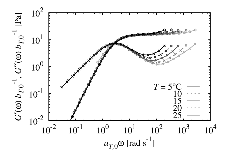
Figure 1:

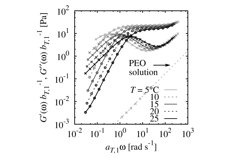
Figure 2:

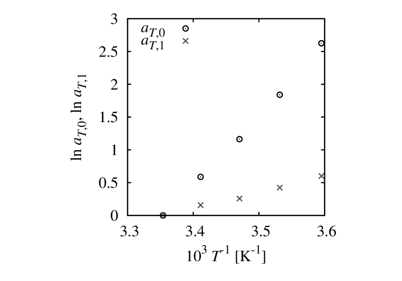
Figure 3:

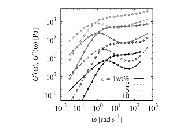
Figure 4:

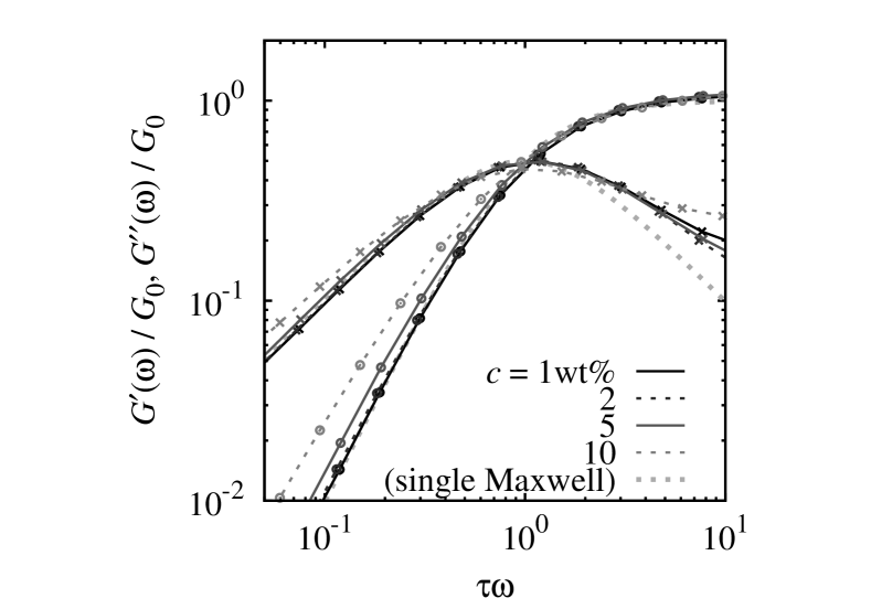
Figure 5:

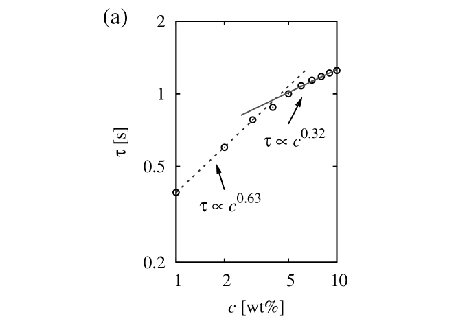
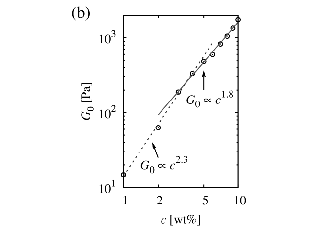
Figure 6:

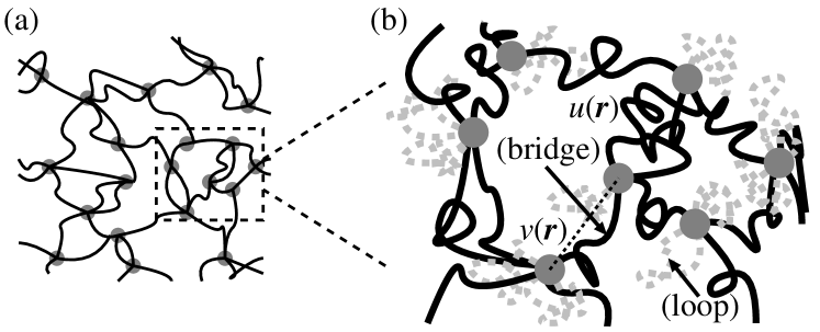
Figure 7:

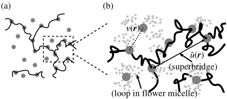
Figure 8:

Figure 9:

References

- Larson (1999) R. G. Larson, The Structure and Rheology of Complex Fluids (Oxford University Press, New York, 1999).
- Annable et al. (1993) T. Annable, R. Buscall, R. Ettelaie, and D. Whittelestone, J. Rheol. 37, 695 (1993).
- Tripathi et al. (2006) A. Tripathi, K. C. Tam, and G. H. McKinley, Macromolecules 39, 1981 (2006).
- Xu et al. (1996) B. Xu, A. Yekta, L. Li, Z. Masoumi, and M. A. Winnik, Colloilds Surf. A: Physicochem. Eng. Asp. 112, 239 (1996).
- Tam et al. (1998) K. C. Tam, R. D. Jenkins, M. A. Winnik, and D. R. Bassett, Macromolecules 31, 4149 (1998).
- Green and Tobolsky (1946) M. S. Green and A. V. Tobolsky, J. Chem. Phys. 14, 80 (1946).
- Tanaka and Edwards (1992) F. Tanaka and S. F. Edwards, Macromolecules 25, 1516 (1992).
- Cathébras et al. (1998) N. Cathébras, A. Collet, M. Viguier, and J.-F. Berret, Macromolecules 31, 1305 (1998).
- Séréro et al. (1998) Y. Séréro, R. Aznar, G. Porte, J.-F. Berret, D. Calvet, A. Collet, and M. Viguier, Phys. Rev. Lett. 81, 5584 (1998).
- Séréro et al. (2000) Y. Séréro, V. Jacobsen, and J.-F. Berret, Macromolecules 33, 1841 (2000).
- Wang (1992) S.-Q. Wang, Macromolecules 25, 7003 (1992).
- Marrucci et al. (1993) G. Marrucci, S. Bhargava, and S. L. Cooper, Macromolecules 26, 6438 (1993).
- Vaccaro and Marrucci (2000) A. Vaccaro and G. Marrucci, J. Non-Newtonian Fluid Mech. 92, 261 (2000).
- Indei et al. (2005) T. Indei, T. Koga, and F. Tanaka, Macromol. Rapid Comm. 26, 701 (2005).
- Indei (2007a) T. Indei, J. Non-Newtonian Fluid Mech. 141, 18 (2007a).
- Indei (2007b) T. Indei, Nihon Reoroji Gakkaishi (J. Soc. Rheol. Jpn.) 35, 147 (2007b).
- Koga and Tanaka (2010) T. Koga and F. Tanaka, Macromolecules 43, 3052 (2010).
- Suzuki et al. (2012) S. Suzuki, T. Uneyama, T. Inoue, and H. Watanabe, Macromolecules 45, 888 (2012).
- Verduin et al. (1996) H. Verduin, B. J. de Gans, and J. K. G. Dhont, Langmuir 12, 2947 (1996).
- Brader (2010) J. M. Brader, J. Phys.: Cond. Mat. 22, 363101 (2010).
- Semenov et al. (1995) A. N. Semenov, J.-F. Joanny, and A. R. Khokhlov, Macromolecules 28, 1066 (1995).
- Khalatur and Khokhlov (1996) P. G. Khalatur and A. R. Khokhlov, Macromol. Theory Simul. 5, 877 (1996).
- Ng et al. (2000) W. K. Ng, K. C. Tam, and R. D. Jenkins, J. Rheol. 44, 137 (2000).
- Bedrov et al. (2002) D. Bedrov, G. D. Smith, and J. F. Douglas, Europhys. Lett. 59, 384 (2002).
- Tae et al. (2002) G. Tae, J. A. Kornfield, J. A. Hubbell, and J. Lal, Macromolecules 35, 4448 (2002).
- Berret et al. (2003) J.-F. Berret, D. Calvet, A. Collet, and M. Viguier, Curr. Opin. Colloid Interface Sci. 8, 296 (2003).
- Castelletto et al. (2004) V. Castelletto, I. W. Hamley, W. Xue, C. Sommer, J. S. Pedersen, and P. D. Olmsted, Macromolecules 37, 1492 (2004).
- Cass et al. (2008) M. J. Cass, D. M. Heyes, R.-L. Blanchard, and R. J. English, J. Phys.: Cond. Mat. 20, 335103 (2008).
- Sprakel et al. (2009) J. Sprakel, E. Spruijt, J. van der Gucht, J. T. Padding, and W. J. Briels, Soft Matter 5, 4748 (2009).
- Mistry et al. (2006) D. Mistry, T. Annable, X.-F. Yuan, and C. Booth, Langmuir 22, 2986 (2006).
- Hansen and McDonald (2006) J.-P. Hansen and I. R. McDonald, Theory of Simple Liquids, 3rd ed. (Elsevier, Amsterdam, 2006).
- van Kampen (2007) N. G. van Kampen, Stochastic Processes in Physics and Chemistry, 3rd ed. (Elsevier, Amsterdam, 2007).
- McPhie et al. (2001) M. G. McPhie, P. J. Daivis, I. K. Snook, J. Ennis, and D. J. Evans, Physica A 299, 412 (2001).
- Uneyama et al. (2011) T. Uneyama, K. Horio, and H. Watanabe, Phys. Rev. E 83, 061802 (2011).
- Evans and Morris (2008) D. J. Evans and G. P. Morris, Statistical Mechanics of Nonequilibrium Liquids, 2nd ed. (Cambridge University Press, Cambridge, 2008).
- (36) S. Suzuki et al., in preparation.
- Abramowitz and Stegun (1972) M. Abramowitz and I. A. Stegun, eds., Handbook of Mathematical Functions with Formulas, Graphs, and Mathematical Tables, 10th ed. (Dover, New York, 1972).
- Tanaka and Koga (2006) F. Tanaka and T. Koga, Macromolecules 39, 5913 (2006).
- Winter and Chambon (1986) H. H. Winter and F. Chambon, J. Rheol. 30, 367 (1986).