The Environmental Dependence of the Incidence of Galactic Tidal Features

Abstract

In a sample of 54 galaxy clusters $(0.04<z<0.15)$ containing 3551 early-type galaxies suitable for study, we identify those with tidal features both interactively and automatically. We find that $\sim$ 3% have tidal features that can be detected with data that reaches a $3\sigma$ sensitivity limit of 26.5 mag arcsec^-2. Regardless of the method used to classify tidal features, or the fidelity imposed on such classifications, we find a deficit of tidally disturbed galaxies with decreasing clustercentric radius that is most pronounced inside of $\sim 0.5R_{200}$. We cannot distinguish whether the trend arises from an increasing likelihood of recent mergers with increasing clustercentric radius or a decrease in the lifetime of tidal features with decreasing clustercentric radius. We find no evidence for a relationship between local density and the incidence of tidal features, but our local density measure has large uncertainties. We find interesting behavior in the rate of tidal features among cluster early-types as a function of clustercentric radius and expect such results to provide constraints on the effect of the cluster environment on the structure of galaxy halos, the build-up of the red sequence of galaxies, and the origin of the intracluster stellar population.

1. Introduction

Galaxies and clusters of galaxies assemble hierarchically, through a long progression of mergers and accretion. As one considers galaxy-scale dark matter halos, baryonic physics becomes more integral and so the analytic formalism developed to calculate the rate of dark matter halo evolution (Press & Schechter, 1974; Bond et al., 1991; Lacey & Cole, 1993), which is broadly confirmed by numerical simulations (Lacey & Cole, 1994; Sheth & Tormen, 1999), becomes less prescriptive. To remedy this shortcoming, galaxy formation is now studied using hydrodynamic numerical simulations (e.g., Springel, 2000; Hoffman et al., 2010), although the details of the assembly process are sensitive both to baryonic physics below scales accessible in the simulations (“sub-grid” physics) and to the complex history that occurs on cosmological scales. Tests of such models include comparisons to the properties of galaxy clusters, their constituent galaxies, and the generation of intracluster stars (Puchwein et al., 2010).

The rate of accretion events and mergers is a fundamental quantity that hierarchical growth models must be able to predict accurately. A proper comparison to an empirical rate measurement is elusive (see Lotz et al., 2011, for a description of the current state of the field). Efforts to measure this rate, particularly as a function of redshift, have focused either on measuring close pairs of galaxies (a few examples include Carlberg, Pritchet, & Infante, 1994; Patton et al., 1997; Le Févre et al., 2000; Kartaltepe et al., 2007; de Ravel et al., 2009), or identifying galaxies that appear morphologically to be the result of ongoing or recent merger events (a few examples include Abraham et al., 1996; Lotz et al., 2008; Jogee et al., 2009; Bridge et al., 2010; Miskolczi et al., 2011) and results often disagree among studies (Lotz et al., 2011). These measurements are difficult, even with the superb angular resolution of the Hubble Space Telescope, for high redshift galaxies. However, renewed focus on identifying tidal features at low redshift has yielded some striking successes both in the increased incidence of detected features (Tal et al., 2009) and their scale and morphologies (Martínez-Delgado et al., 2010).

We aim to make a measurement of the major merger rate at low redshift, but as a function of environment. A complication in practice is that the definition of a major, vs a minor, merger is typically made on the basis of the mass ratio between the two galaxies. Such a definition is difficult to apply empirically, particularly in environments that may have affected the individual galaxies and in cases where the two initial galaxies have merged into a single remnant. We define a major merger here as one that results in the large-scale tidal features we are searching for around luminous, early-type ($R^{1/4}$ profile) galaxies. Although this approach evidently complicates comparisons to models, it should not impact our primary goal of searching for patterns in the occurrence of tidal features as a function of environment.

Dubinski, Mihos, & Hernquist (1999) showed how the dark matter halo structure of the merging galaxies can significantly alter the appearance of a major merger, thereby demonstrating that measurements of major merger signatures, even at a single redshift, could be a sensitive model diagnostic. Beyond the purpose of understanding hierarchical accretion better, we need to study the merger rate in clusters and in the surrounding environments because these events contribute stars to the ubiquitous intracluster stellar population (Zibetti et al., 2005; Gonzalez, Zabludoff, & Zaritsky, 2005), which is an important component in estimates of the baryon budget of groups and clusters (Gonzalez, Zaritsky, & Zabludoff, 2007; Giodini et al., 2009; McGee & Balogh, 2010), and calculations of the chemical enrichment history of the intracluster medium (Zaritsky, Gonzalez, & Zabludoff, 2004; Sivanandam et al., 2009). Furthermore, extending any study of galaxies within clusters out to the surrounding environs is critical because differences in their star formation histories, which could be related to interactions, begin to appear at clustercentric radii of several Mpc (Lewis et al., 2002; Gomez et al., 2003).

The principal observational challenge in identifying tidal features is that such features are of low surface brightness and have irregular morphologies. A variety of techniques have been developed to identify merging galaxies and mergers (e.g., Conselice et al., 2003; Lotz et al., 2008), but the problem takes on different forms depending on the redshift of the galaxies and the depth and uniformity, or “flatness”, of the data. For galaxies in the local universe, Colbert et al. (2000) employed unsharp masking (subtracting a smoothed image of the galaxy from itself), galaxy model division (dividing the galaxy image by a best-fit model galaxy made from nested elliptical isophotes), and color mapping (division of the galaxy image in one color band by the galaxy image in another color band) to aid in the visual detection of tidal features and found that 41% (9 of 22) of analyzed isolated galaxies show tidal features, while only 8% (1 of 12) of group galaxies had such features. While this result is certainly suggestive of lower rates of tidal features in group environments than in the field, Poisson statistics limits the significance of the discrepancy to less than $2\sigma$. Van Dokkum (2005) divided his galaxy images by a model fit and measured the mean absolute deviation of the residuals to define a quantitative threshold for the identification of tidally disturbed galaxies. He found that 53% of his sample of 126 red, field galaxies show tidal features, while 71% of the bulge-dominated early-type subset of 86 galaxies appear to be tidally disturbed. Using a similar method for a sample of nearby, luminous, elliptical galaxies, Tal et al. (2009) found that 50% (5 of 10) of cluster galaxies, 62% (13 of 18) of poor-group galaxies, and 76% (16 of 21) of isolated galaxies have tidal features. Similar to the results of Colbert et al. (2000), these also suggest that tidal features are less common in cluster environments than in the field, but again the significance of the result is limited by the sample size. Janowiecki et al. (2010) quantify the extent of tidal substructure in five elliptical galaxies in the Virgo cluster by measuring the luminosity of the substructure and find no obvious correlation between clustercentric radius and the amount of substructure. Larger samples are needed to resolve this issue.

Larger samples studied thus far are from field surveys. Bridge et al. (2010) visually identify tidal tails in a sample of 27,000 galaxies over 2 square degrees of the Canada-France-Hawaii Telescope Legacy Deep Survey (CFHTLS-Deep) to find that the merger fraction of galaxies evolves from 4% at $z\sim 0.3$ to 19% at $z\sim 1$. Miskolczi et al. (2011) study a sample of 474 galaxies selected from the SDSS DR7 archive to find that at least 6% of the galaxies have distinct tidal streams and a total of 19% show faint features. No large samples have included substantial numbers of galaxies in dense environments.

Deep, uniform imaging is a prerequisite for any such study. The incidence of identified mergers among field galaxies increases from $<$ 10% locally in relatively shallow imaging (Miskolczi et al., 2011) to many tens of percent in deeper imaging (Martínez-Delgado et al., 2010; Tal et al., 2009). For this and other reasons, it is neither surprising nor incorrect that the apparent total rates from different studies vary widely. The key is therefore to compare within a given study rather than across studies.

We identify tidally disturbed galaxies in the largest existing sample of deep, wide-field images of nearby galaxy clusters $(0.04<z<0.15)$. These come from the Multi-Epoch Nearby Cluster Survey (MENeaCS; Sand et al., 2012), and this study is part of a series using those data to address a series of science questions including so far the incidence of intracluster supernovae (Sand et al., 2011), the rate of SNe Ia in clusters (Sand et al., 2012), the evolution of the dwarf-to-giant ratio (Bildfell et al., 2012), and the rate of SNe II’s in clusters (Graham et al., 2012). The larger sample size enables us to examine, for the first time, relative rates of tidal features as a function of different measures of the global environmental (projected clustercentric radius) and local environment (projected local galaxy density). In §2 we briefly present the data we use and discuss our analysis of these data, including the selection of candidate cluster galaxies and the calculation of the tidal parameter. In §3 we present our results and discuss whether any significant trends are identified. We present our conclusions in §4. We adopt $H_{0}=71$ km s^-1 Mpc^-1, $\Omega_{M}=0.27$, and $\Omega_{\Lambda}=0.73$ for conversions to physical units.

2. Data and Analysis

2.1. The Cluster Sample

The galaxy cluster images used for this study are the deep stack images obtained by the Multi-Epoch Nearby Cluster Survey of X-ray selected clusters (MENeaCS; Sand et al., 2012) with MegaCam on the Canada-France-Hawaii Telescope (Boulade et al., 2003). The image stacks typically contain 20 to 30 120-second exposures in the $g^{\prime}$ and $r^{\prime}$ filters for each cluster, observed at a monthly cadence to pursue the supernovae science goals (Sand et al., 2011, 2012). The analysis is done on the deeper $r^{\prime}$ data. The depth of the $r^{\prime}$ image stacks for point source detection corresponds to limiting absolute magnitudes of $-$11 to $-$13 at the distance of the clusters. The $3\sigma$ limiting apparent surface brightness, derived from the sky RMS, of 1 arcsec² patches in the deep stack images is approximately 26.5 mag arcsec^-2. The faintest tidal features that we visually identify are approximately this magnitude (see Fig. 7 and 8). MegaCam features a large field of view ($\sim$1 degree²) that enables us to search for tidal features from the central regions out to $1-2R_{200}$ and study the radial and environmental dependence of the merger rate. Details on the cluster parameters and image reduction process are given in Sand et al. (2011, 2012). The list of the 54 clusters analyzed is given in Table 1. The cluster redshifts range from $0.04<z<0.15$, with the redshifts taken from the NASA Extragalactic Database.

Table 1Galaxy Clusters

Cluster	Redshift	$L_{X,0.1-2.4keV}$	${M_{200}}$	${R_{200}}$	$N_{gal}$	$N_{gal}$	$N_{gal}$
		($10^{44}$ ergs/s)	($M_{\odot}$)	(Mpc)	Analyzed	Visual Sample	Cleaned-auto sample
Abell1033	0.126	5.12	7.28	1780	72	2	1
Abell1068	0.138	5.94	8.13	1840	99	11	2
Abell1132	0.136	6.76	7.44	1790	107	8	2
Abell119	0.044	3.30	5.14	1630	32	0	3
Abell1285	0.106	4.66	6.76	1750	93	15	4
Abell133	0.057	2.85	4.78	1580	38	2	1
Abell1348	0.119	3.85	5.94	1670	71	3	2
Abell1361	0.117	4.95	7.09	1770	57	2	1
Abell1413	0.143	10.83	12.45	2120	153	5	0
Abell1650	0.084	5.66	9.18	1950	72	5	0
Abell1651	0.085	6.92	10.48	2040	44	5	2
Abell1781	0.062	3.79	5.73	1680	30	1	2
Abell1927	0.095	2.30	4.08	1490	62	0	0
Abell1991	0.059	1.42	2.86	1340	26	2	2
Abell2029	0.077	17.44	16.57	2380	75	4	2
Abell2033	0.082	2.55	4.38	1530	76	2	0
Abell2050	0.118	2.63	4.54	1530	86	6	3
Abell2055	0.102	3.80	5.83	1670	54	1	1
Abell2064	0.108	2.96	4.92	1570	55	1	4
Abell2069	0.116	3.45	5.49	1630	124	3	1
Abell21	0.095	2.64	4.51	1540	43	2	4
Abell2142	0.091	21.24	19.56	2510	130	1	2
Abell2319	0.056	15.78	15.61	2350	24	3	2
Abell2409	0.148	7.57	9.69	1950	88	0	0
Abell2420	0.085	4.64	6.67	1760	64	0	3
Abell2426	0.098	4.96	7.04	1780	88	0	1
Abell2440	0.091	3.36	5.33	1630	63	0	0
Abell2443	0.108	3.22	5.22	1600	46	0	1
Abell2495	0.078	2.74	4.58	1550	37	0	1
Abell2597	0.085	6.62	8.62	1910	39	0	3
Abell2627	0.126	3.25	5.29	1600	80	0	0
Abell2670	0.076	2.28	4.03	1490	51	0	3
Abell2703	0.114	2.72	4.64	1540	86	1	2
Abell399	0.072	7.06	8.15	1880	89	4	9
Abell401	0.074	12.06	13.02	2200	82	5	5
Abell553	0.066	1.83	3.43	1410	12	3	2
Abell644	0.070	8.33	10.02	2020	23	2	2
Abell646	0.129	4.94	6.47	1710	61	1	2
Abell655	0.127	4.90	6.54	1720	97	1	0
Abell7	0.106	4.52	6.61	1740	29	0	1
Abell754	0.054	7.00	10.11	2040	47	3	3
Abell763	0.085	2.27	4.03	1480	40	2	3
Abell780	0.053	4.78	6.72	1780	22	1	0
Abell795	0.136	5.70	7.89	1820	107	5	5
Abell85	0.055	9.41	10.27	2050	47	3	2
Abell961	0.124	3.12	5.13	1590	106	3	3
Abell990	0.144	6.71	8.88	1890	147	2	4
MKW3S	0.045	3.45	4.09	1510	12	0	1
ZwCl1023	0.143	4.71	6.92	1740	81	1	3
ZwCl1215	0.075	5.17	7.27	1810	55	0	0

Note. — Basic properties of clusters analyzed along with the total number of galaxies and number in the visual and cleaned-auto samples of disturbed galaxies for each cluster.

2.2. Selecting Elliptical Cluster Galaxies

We use SExtractor, a source detection algorithm (Bertin & Arnouts, 1996), in two-image mode to measure the magnitudes and colors of all galaxies in the images. The galaxy clusters are relatively nearby ($z<0.15$) and we can only detect tidal features in galaxies of relatively large angular extent (many arcsec), so we select for further study only sources that have a minimum area of 60 pixels that are each at least 6$\sigma$ above the background and have a stellarity parameter of less than 0.05. Using that output, we create color magnitude diagrams for each cluster using the absolute magnitudes derived from SExtractor’s AUTO_-MAG parameter, which uses an aperture radius of $2.5r_{Kron}$ (Kron, 1980), and the color using the APER_-MAG parameter, which finds the magnitude within a small aperture we set to 1.9” in diameter in order to maintain high S/N and limit contributions from neighboring sources.

To identify a sample of galaxies with a high probability of being at the cluster redshift and to avoid star-forming, late-type galaxies that can have significant internal structure, we select red sequence galaxies for further study. To do this, we first visually examine the location of galaxies in the color-magnitude diagram that are within 1.5 arcmin of the cluster center. Using these galaxies, we define the color normalization of the red sequence and adopt an empirically-determined slope of $-$0.033. The red sequence slopes of clusters at a given z show little if any scatter (Ellis et al., 1997; Stanford et al., 1998; Gilbank et al., 2008). We select galaxies with colors within $\pm 0.13$ of the mean relation for further study. This estimate of the color scatter is probably somewhat conservative (for example, Bildfell et al. (2012) select galaxies within $\pm 0.2$ of the red sequence), but it minimizes contamination, which for this study is more important than completeness. A tight color selection could result in a bias if interacting galaxies are bluer than the mean, but (as we find later) they are not. We do not explicitly apply k-corrections or evolution corrections, but they are inherent in our red-sequence color selection. We repeat the procedure of visually identifying the optimal zero point for each cluster, keeping the slope and thickness of the color-magnitude band constant. We then apply these cuts to the entire image, keeping only galaxies with $M_{r}<-20$ (where $M_{r}$ is simply the sum of the apparent magnitude and the distance modulus) at the cluster redshift (see Fig. 1 for a sample color-magnitude diagram and galaxy selection) to ensure that the candidate galaxies are sufficiently luminous for our tidal analysis. We will discuss estimates of the interloper fraction in §3.2.

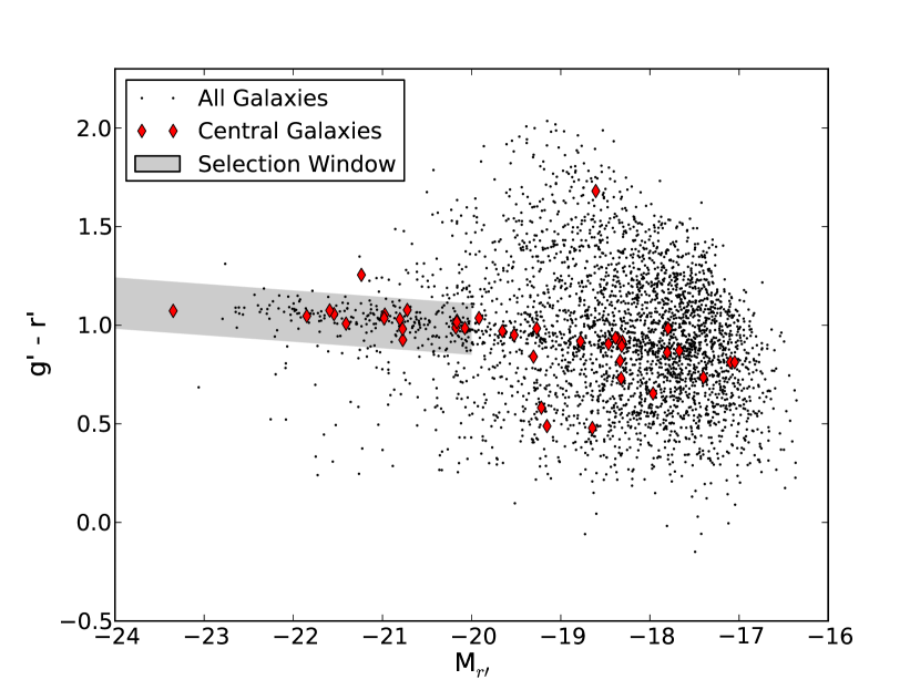
Figure 1.— Sample color magnitude diagram (Abell 21). The black dots represent all galaxies meeting our SExtractor selection parameters. The red diamonds are galaxies located within 1.5’ of the cluster center used to originally define the location of the cluster red sequence. Galaxies within the shaded region are brighter than our minimum magnitude and are identified as red sequence members of the cluster. These are the galaxies in which we search for tidal features.

We focus our study on elliptical galaxies because their surface brightness distributions can be modeled more easily than those of spirals and because disk galaxies are believed to not have been involved in major mergers since moderate redshifts unless both progenitors were gas rich, a condition that will be rare in these high density environments (Robertson et al., 2006). To limit our sample to elliptical galaxies, we reject galaxies with ellipticity greater than 0.5 and we discriminate based on the shape of the surface brightness profile. To do the profile discrimination, we select the radial region of the galaxy’s surface brightness profile in which the intensity is less than 10% of the galaxy’s peak intensity (to avoid the exponential bulge of spirals) and greater than $1\sigma$ above the background sky level. We reject galaxies that have a lower $\chi^{2}$ for the weighted least squares linear fit of $\ln$(intensity) vs. radius than of $\ln$(intensity) vs $r^{1/4}$ (Fig. 2). Out of the initial sample of 11,904 red sequence galaxies, 4526 were flagged as disks due to their surface brightness profiles and 2322 galaxies were flagged as disks due to their ellipticity, with a union of the two criteria resulting in a total of 5486 galaxies being dropped from the initial sample. We found with visual examination that only $\sim 3\%$ of galaxies classified as ellipticals had obvious spiral structure (these are later discarded from the final sample). It is more difficult to estimate the fraction of galaxies identified as disks that are actually ellipticals due to the similar morphology of E and S0 galaxies, but the vast majority of the galaxies identified as disks did visually appear to be correctly flagged. There were some instances ($<1$% of all galaxies) where obvious mergers were classified as disks, but these tended to be galaxies that still had an obvious disk component and/or lacked a clear nucleus.

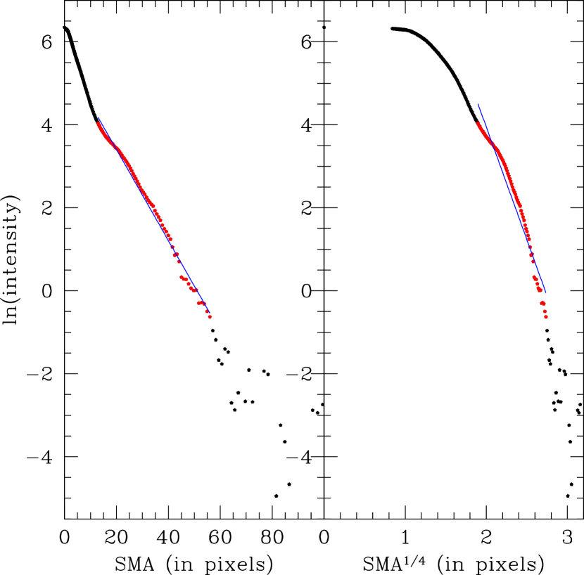
Figure 2.— Sample luminosity profile fit used to identify a spiral galaxy. The linear least-squares fit of the ln(intensity) versus semi-major axis (left panel) has a smaller $\chi^{2}$ profile than the least-squares fit of the ln(intensity) versus semi-major axis^1/4. The portions of the luminosity profile used for the best fits are shown in red, the portions excluded are shown in black. The blue lines are the best fit linear regression lines.

For the subsequent analysis, we extract image regions of width corresponding to seven times each galaxy’s diameter (as determined by SExtractor). The sizes of these images range from 46 arcmin² for the largest central galaxies to 500 arcsec² for the smallest galaxies that meet our thresholds, with the median size being 1 arcmin². The angular sizes translate into 850$\times$850 kpc to 50$\times$50 kpc with the median area being 105$\times$105 kpc. The sizes of the images were chosen to ensure that any possible extended tidal tails would be included in the analysis and that in almost all cases there is sufficient area to accurately define a background sky level. Visual examination did not reveal any cases where tidal features began beyond the analyzed image region. Though there are a few cases where large tidal features continue beyond the analyzed image region, these galaxies are still correctly identified as tidally-disturbed by both the visual and automated selections.

2.3. Calculating the Tidal Parameter

In studies of mergers and merger remnants there is always a tension between visual and automated identification. Visual approaches have the advantage that they harness the tremendous pattern recognition skills that the human eye has evolved, but suffer from non-uniformity among different practitioners, and poorly defined criteria. Automated approaches are repeatable and well-defined, the latter being particularly important for comparisons to models, but are likely to be less powerful in selecting varying morphologies within this ill-defined class of objects. We resolve this conflict by applying both approaches.

To objectively determine whether a galaxy is tidally-disturbed we follow the general procedure presented by Tal et al. (2009) (shown in Fig. 3) to calculate a tidal parameter from the average residual of the galaxy image divided by its best fit model. First a background gradient is fit and subtracted from each galaxy image using the BACKGROUND generated by SExtractor with BACK_-SIZE = 64 and BACK_-FILTERSIZE = 3, in order to minimize large scale gradients across the galaxy images caused by intracluster light or nearby bright galaxies. The BACKGROUND map generated by SExtractor is a bicubic spline interpolation over the sigma-clipped pixels in the area of the BACK_-SIZE parameter median-filtered over the BACK_-FILTERSIZE number of BACK_-SIZE areas. The BACK_-SIZE parameter is chosen for our pixel scale (0.187”/pixel) to be larger than the scales of typical tidal features.

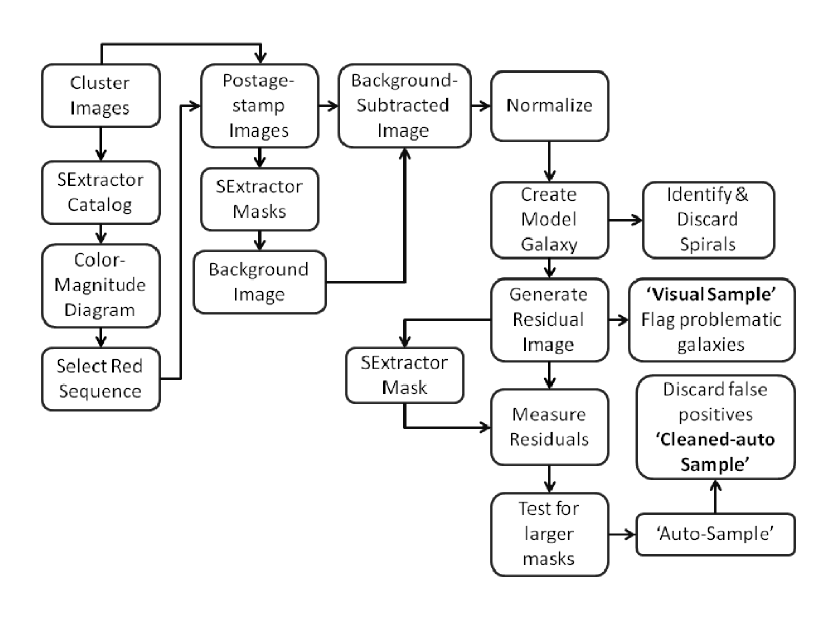
Figure 3.— Flow chart showing process by which samples of tidally-disturbed galaxies are identified.

The tidal parameter analysis is very sensitive to unmasked sources, which are easily confused with tidal matter. Pixels with known objects are masked using the SExtractor object catalog. To optimize masking of background sources while minimizing masking of real tidal features, we create our masks from the union of two different masking catalogs. One catalog targets large galaxies using DETECTMIN_-AREA $=$ 5, DETECT_-THRESH $=$ 1.8, and DEBLEND_-MINCONT $=$ 0.001 to only mask very significant sources well removed from the subject galaxy. These parameters require DETECTMIN_-AREA number of neighboring pixels to be DETECT_-THRESH sigma above the background in order to be detected as an object. The DEBLEND_-MINCONT parameter determines if a cluster of pixels above the detection threshold should be divided into multiple sources, and has been tuned here to differentiate only very distinct clumps as separate objects. A second, more aggressive catalog targeting stars is generated by only identifying objects with CLASS$\_$STAR less than 0.05 with DETECT_-THRESH $=$ 1.4, and DEBLEND_-MINCONT $=$ 0.0001 (a lower deblending contrast to more readily identify stars blended with the target galaxy). We also create a background sky frame to be used in a noise correction term (described below) using a third, very agressive catalog generated with DETECT_-THRESH $=$ 0.8, and DEBLEND_-MINCONT $=$ 0.001 that masks all sources (including the target galaxy and associated tidal features). Unmasked pixels are randomly chosen to replace the masked pixels in the creation of a background image in order to preserve the noise characteristics of the original image.

We create a best-fit model for each galaxy using the IRAF tasks ellipse and bmodel. We fix the isophotal center but allow for variable position angle and ellipticity as a function of semi-major axis to generate best-fit isophotes out to 80% of the postage stamp image dimensions, and then create the corresponding model galaxy. The model image covers the entire postage stamp area, with pixel values set to zero beyond the area covered by the best fit model. Pixels whose model value exceeds 0.01 times the peak value at the galaxy center are masked so that the analysis focuses on any extended tidal features rather than residuals near the galaxy nucleus that may arise from slight misplacement of the galaxy center in the model. The masked galaxy image is then divided by the model image. The residual image is median filtered with a 5$\times$5 pixel kernel in order to facilitate visual identification of tidal features. We further supplement our pixel mask by running SExtractor on the smoothed residual image with DETECTMIN_-AREA $=$ 5, DETECT_-THRESH $=$ 5, and DEBLEND_-MINCONT $=$ 0.0001 primarily in order to mask faint galaxies close to the primary galaxy. The final mask for a typical galaxy includes 5-20% of the pixels in the area over which the model is computed. We discard all galaxies that have over 50% of the image area masked. This should not bias the results unless real tidal features are being masked (which we visually verified is very uncommon, with only a few cases out of several thousand galaxies). We also confirm with a control sample that the masking is not responsible for the radial trend we discuss below (see §3.2). With the enhanced mask we repeat the process of creating a model galaxy and smoothed residual image.

We examine all galaxy and residual images for quality and calculate the tidal parameter. We visually inspect and discard the galaxy and corresponding residual images that are contaminated with unmasked diffraction spikes from bright stars. We also flag galaxies that have visible tidal structure. This latter sample is referred to as our visual sample. We then generate an auto-detected sample using a tidal parameter that is calculated by finding the mean of the absolute value of the final residual image:

$$T_{galaxy}=\overline{\bigg{|}\frac{I_{x,y}}{M_{x,y}}-1\bigg{|}}$$ (1)

where I_x,y is the pixel value at x,y of the object frame and M_x,y is the pixel value at x,y of the model frame. A background-noise correction frame is created by adding the background sky image created earlier to the model image and then dividing by the model. The resulting frame is then median filtered and a tidal parameter is recalculated for the model plus noise frame. The final tidal parameter, corrected for noise, is then found as follows:

$$T_{c}=\sqrt{T_{galaxy}^{2}-T_{model}^{2}}$$ (2)

This tidal parameter is particularly sensitive to deviations when the model values are small. Because our models often go to zero toward the image edges, we find that we increase the relative stability of our tidal parameters by first dividing the galaxy images by their mean background counts so that all images have a pedestal of 1 count.

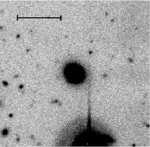
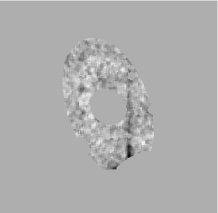
Figure 4.— Example of galaxy in Abell 795 discarded interactively due to unmasked diffraction spike. Left column: galaxy image displayed with 15” scale bar. Right column: residual of galaxy image divided by model with galaxy core and neighboring external objects masked. The tidal parameter used to select tidally-disturbed galaxies uses the mean value of the unmasked areas of this image together with a noise correction frame.

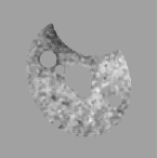
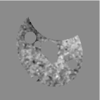
Figure 5.— Sample galaxy in Abell 795 automatically discarded due to extended light profile of bright nearby galaxy. Galaxies whose tidal parameters decrease by more than 5% when the mask sizes for bright sources are increased by 10% are discarded as this is an indication that the high tidal parameter is likely due to extended light from neighboring bright sources rather than from tidal features. Left panel: Galaxy image shown with 15” scale bar, center: residual image, right: residual with larger masking. Percent change in tidal parameter with larger masking: $-$16%.

The calculation of a tidal parameter does not by itself identify a set of tidally disturbed galaxies because there is no absolute reference. We define a threshold $T_{c}$ parameter that is best matched to what we visually identify as tidally disturbed galaxies. The correspondence is not perfect, as we describe further below, but we settle on defining those galaxies with $T_{c}>9\times 10^{-4}$ as tidally-disturbed. We find that many galaxies have higher values for the tidal parameter because light from the extended haloes of nearby bright galaxies extends beyond the mask. In an effort to eliminate these false-positives we reject from our analysis candidate tidally-disturbed galaxies whose tidal parameters decrease by more than 5% when the mask sizes for bright sources are increased by 10% (e.g. Fig. 5). While it is true that this filter is biased against galaxies in dense regions, it would only bias our results if real tidal features are being masked by the increased mask sizes. We verified that the fraction of discarded galaxies that were visually-disturbed was consistent (within statistical errors) with the fraction of all galaxies that are visually-disturbed within a given radial bin, indicating that these filters do not introduce a radial trend. The remaining galaxies with $T_{c}>9\times 10^{-4}$ make up the auto-detected sample of tidally-disturbed galaxies. Lastly, because some false positives arise due to image quality issues, unmasked sources, and diffuse light gradients from nearby bright galaxies, we visually inspect this sample to construct our cleaned-auto-detected sample of tidally-disturbed galaxies. The procedure we have just described consists of many steps, all of which affect the number of systems that will ultimately be classified as mergers, and thereby complicate comparison to models on an absolute scale. However, these filters should be mostly insensitive to clustercentric radius, particularly outside the crowded central part of a cluster right near the brightest cluster galaxy, and as such are not expected to affect our results.

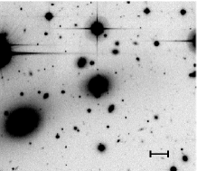
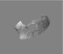
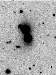
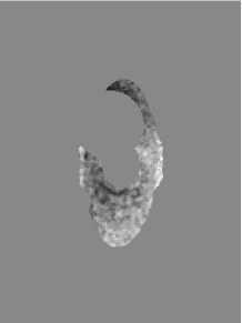
Figure 6.— Sample galaxies flagged as disturbed in the auto-sample, but excluded from the cleaned-auto sample in Abell 553 (top) and Abell 401 (bottom). Left column: galaxy images displayed with 15” scale bars, right: region used for the residual calculation that has the ellipticity of the primary galaxy and has regions masked. Top panel: it is not clear whether these two galaxies are interacting or are a close superposition. The high mean residual value appears to be primarily caused by light from the adjacent galaxy spilling beyond its mask rather than any visible tidal structure ($T=1.4\times 10^{-3}$). Bottom panel: the high residual value appears to be primarily due to the extended light profile of a nearby giant elliptical galaxy ($T=1.8\times 10^{-3}$).

3710 galaxies satisfy all of the automated selection criteria (cluster color-magnitude band, $M_{r^{\prime}}<-20$, $r^{-1/4}$ radial brightness profile, successful IRAF $bmodel$ generation, and less than 50% of the area surrounding the galaxy masked). Of these, we discard 79 that are problematic due to masking issues and background light gradients (e.g. Fig. 4). Of the remaining 3631 galaxies, 202 were flagged as potentially-disturbed by our tidal parameter threshold, while 109 galaxies were visually-identified as tidally-disturbed (see Figures 7 and 8 for examples). While there are a large number of disturbed galaxies that the automated sample identified that were missed by the visual inspection (see Fig. 8 for an example), the sample also includes many false identifications (usually due to image quality problems or unmasked sources). By eye we discard obvious false detections from the automated sample to make a cleaned-auto sample of 122 galaxies (see Fig. 6) out of 3551 total galaxies (hereafter referred to as “all”). The samples are compared below.

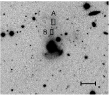
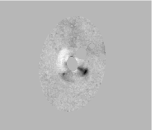
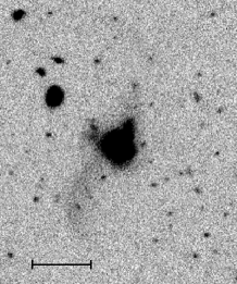
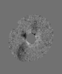
Figure 7.— Examples of galaxies marked as disturbed in both the visual and cleaned-auto samples in Abell 21 (top) and Abell 1068 (bottom) . Left column: galaxy images displayed with 15” scale bars, right: region used for the residual calculation that has the ellipticity of the primary galaxy and has regions masked. Top panel: the galaxy is clearly undergoing a merger; note the bright shell below the galaxy and the diffuse tidal stream above the galaxy ($T=1.2\times 10^{-3}$). The mean surface brightness within the red box “A” is 25.4 and within box “B” is 25.1. Bottom panel: also a clear case of a recent or ongoing merger with a distinct tidal tail extending to the lower left of the galaxy and tidal debris to the left and above the galaxy ($T=1.1\times 10^{-3}$). Galaxies that are identified by both the visual and cleaned-auto samples tend to have the strongest and most distinctive tidal features.

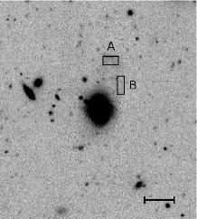
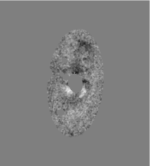
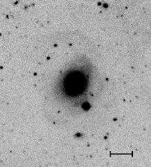
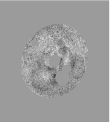
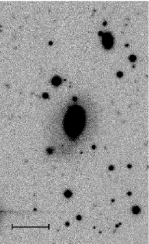
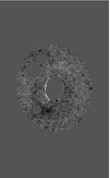
Figure 8.— Examples of galaxies in either the visual or cleaned-auto samples (but not both) in Abell 399 (top and middle panels) and Abell 553 (bottom). Left column: galaxy images displayed with 15” scale bars, right: region used for the residual calculation that has the ellipticity of the primary galaxy and has regions masked. Top panel: Sample galaxy flagged as disturbed in the visual sample, but not in the cleaned-auto sample ($T=8.6\times 10^{-4}$). Note the ring of tidal debris extending from the top region of the galaxy. The mean surface brightness within the red box “A” is 25.7 and within box “B” is 26.3. Middle panel: Another sample galaxy flagged as disturbed in the visual sample, but not in the cleaned-auto sample ($T=7.1\times 10^{-4}$). Note the series of tidal shells. Bottom panel: Sample galaxy flagged as disturbed in the cleaned-auto sample, but not in the visual sample ($T=9.1\times 10^{-4}$). Note the diffuse shell extending from the lower left portion of the galaxy.

3. Results

3.1. Rates of Tidal Features

The intersection of the visual and cleaned-auto samples includes 42 galaxies, while the union of the two samples includes 189 galaxies. There is no single characteristic that uniquely determines whether a galaxy is identified or missed by the visual or cleaned-auto samples. The visual sample includes galaxies that have tidal features that are close to ellipsoidal, of smaller spatial extent, or of such low surface brightness that they are missing from the cleaned-auto sample. The cleaned-auto sample includes galaxies whose residual images show strong features that were not included in the visual sample because it was not evident whether these are actual tidal features, spiral arms, or nearby satellite galaxies. There are also a few instances of the cleaned-auto sample missing galaxies whose features are very prominent, because these have been masked as separate sources by SExtractor. The intersection sample tends to include the strongest, most spectacular features, while the union is a more complete sample, but suffers from a larger fraction of questionable detections.

The tidal feature rate among early-type galaxies in these environments, using the cleaned-auto and visual samples, is $3.4\pm 0.3\%$ and $3.0\pm 0.3\%$, respectively, where the uncertainties are purely statistical. The union of the two samples results in a rate of $5.3\pm 0.4\%$. As we mention in §2.2 a tight color selection could result in a bias if interacting galaxies are bluer than the mean. The mean color offset from the red sequence is $0.00\pm 0.07$ for the visually-selected sample and $-0.01\pm 0.06$ for the cleaned-auto sample, while the mean color offset for all galaxies analyzed is $0.00\pm 0.06$, demonstrating that our interacting samples do not suffer from a color bias. The rate of tidally disturbed cluster galaxies we find is significantly lower than the rate observed by Tal et al. (2009), but the difference is likely because our sample is $\sim$ an order of magnitude more distant, resulting in the smaller apparent size of galaxies and their associated tidal features. Our rates match more closely those of Bridge et al. (2010) and Miskolczi et al. (2011), although again it is complicated to compare results among studies.

Although the measured rate of tidal features appears small at first, some minor adjustments can lead to an inference that the majority of the initial cluster elliptical population must have experienced a major merger. First, the $\sim$ 3% rate, implies that at least 6% of the initial population experienced a merger because a merger involves two galaxies. If one then considers that the tidal signatures will not last indefinitely the numbers rise again. If, for example, tidal features last 2 Gyr (Quinn, 1984) then the rate of mergers increases by a factor of about 5 to $\sim 30\%$. If one further considers that mergers were probably more likely in the past, then the number rises even more. None of this is empirically well determined, but our fundamental conclusion is that our low rate measurement does not necessarily imply a low incidence of mergers over the lifetime of these galaxies.

3.2. Interlopers and Projection Effects

Before proceeding to examine the spatial distribution of galaxies with tidal features, we stop to consider the effect of interloping galaxies on our radial trends. Without spectroscopic redshifts, we do not know with certainty whether or not a particular galaxy is in the cluster. This acts to muddle any real correlations with radius. To estimate the effect of interlopers within our color-selected samples, we count the number of galaxies selected using color-magnitude bands of the same size displaced redward by 0.26 mag (the thickness of our selection area). These displaced color-magnitude bands contain 2834 galaxies, while the bands centered on the red sequences contain 11,904 galaxies, suggesting that approximately 80% of our selected galaxies are cluster members. We also count the number of galaxies in the four deep fields of the CFHTLS (Gwyn, 2008) that would satisfy our galaxy selection criteria. The count from the CFHTLS-Deep fields yielded a much lower estimation of the number of interloping galaxies, but had large field-to-field variation. Therefore, we conservatively use the interloper estimate from the displaced color-magnitude bands and repeat our tidal parameter analysis for these redder galaxies to determine what effect they may have on the results. A higher fraction of the background galaxies are ellipticals, because we are dealing with brighter and redder galaxies, resulting in a slightly higher fraction of these (34% versus 30% of the cluster sample) meeting all selection criteria and contributing to the final results. As expected for a background population, the fraction of interlopers that are tidally disturbed does not correlate with clustercentric radius — demonstrating that crowding toward the center of the cluster does not artificially create a radial effect. However, interlopers are a larger fraction of our “cluster” sample at larger clustercentric radii (as high as 45% beyond $R_{200}$ vs less than 10% within $R_{200}$) due to the steep decrease in the number density of actual cluster galaxies at larger clustercentric radii. The background galaxies have slightly higher rates of tidal features ($4.3^{+0.8}_{-0.7}\%$ visually-detected and $4.5^{+0.8}_{-0.7}\%$ auto-detected, with the statistical uncertainties calculated using the Poisson single-sided limits from Gehrels (1986)) than the cluster sample ($3.1\pm 0.3\%$ visually-detected and $3.3\pm 0.3\%$ auto- detected) suggesting that they might slightly influence any radial behavior.

3.3. Clustercentric Radius

To examine the rates of tidal features as a function of projected clustercentric radius, we rescale the projected radii using the $R_{200}$ value of each cluster from Sand et al. (2012). These radii were estimated using the conversion between $L_{X}$ and $M_{200}$ found by Reiprich & Böhringer (2002) and the correspondence between $M_{200}$ and $R_{200}$. Clustercentric radii are measured from the brightest cluster galaxy (though we verified that the results do not change significantly when the radii are measured from the X-ray center).

Not all clusters are sampled to the same normalized projected clustercentric radius, so we consider different subsamples. We create a first subsample of the 1657 galaxies within $R_{200}$ in the 50 clusters for which our survey is complete out to $R_{200}$, a second subsample of the 1540 galaxies within $2R_{200}$ in the 26 clusters for which we are complete to $2R_{200}$, and a combined sample of all galaxies within $R_{200}$ in clusters complete to $R_{200}$ and all galaxies within $2R_{200}$ in clusters complete to $2R_{200}$. In Figure 9 we plot the relative radial distributions of “all” galaxies and our various samples of galaxies with tidal signatures.

The distributions shown in Figure 9 make clear that there is a significant deficit of galaxies with tidal signatures towards the centers of these clusters. The deficit is evident within $\sim 0.5R_{200}$, which is well outside an area about the brightest central galaxy where one might expect that confusion could lead to lower detection rates. In fact, as we find with a control sample of background galaxies that shows no gradient in tidal features, we are not affected by confusion in the center of these clusters (§3.2). Finally, these findings are independent of whether visual or automated techniques are utilized.

Figure 9.— Histograms of galaxies versus projected clustercentric radius. The left section is the sample of 50 clusters for which the survey is complete within $R_{200}$, whereas the right section is the sample of 26 clusters complete within $2R_{200}$. Top panel: “all” galaxies, 2nd panel down: visually-selected disturbed galaxies, 3rd panel down: cleaned-auto sample of disturbed galaxies, 4th panel down: union of visually and cleaned-auto-selected galaxies, bottom panel: intersection of visually and cleaned-auto-selected galaxies.

To place these conclusions on a more solid statistical footing, we apply K-S tests to evaluate the likelihood that the cumulative distributions of galaxies with tidal features are drawn from the parent distribution of “all” galaxies. For the sample complete within $R_{200}$ we find that the tidal sample was not drawn from the parent sample with 98.2% confidence for the visually-selected sample, 91.5% confidence for the automated selection, 94.5% for the intersection of the two samples, and 97.4% for the union. For the sample complete to $2R_{200}$, the confidence limits fall below $2\sigma$ significance.

The radial variations in the incidence of tidal signatures suggests that either (or both) the creation or destruction of tidal features depends on clustercentric radius. More appropriately, the variation depends on a physical characteristic that drives the phenomenon and which is itself correlated with clustercentric radius. A straightforward hypothesis is that tidal signatures are more easily erased in a dense environment due to shorter dynamical times. While this is likely to be true near the center of the clusters, where the intracluster light is built up, by the time one is considering galaxies at $R_{200}$ and beyond, it may seem unlikely that the global potential will strip tidal material.

To test this hypothesis, we rely on numerical simulations by Rudick et al. (2009) that find that the decay time of tidal streams is approximately 1.5 times the dynamical time at their location in the cluster. The dynamical time at clustercentric radius $r$ is given by,

$$t_{dyn}=\frac{\pi}{2}\sqrt{\frac{r^{3}}{GM}}$$ (3)

where $M$ is the mass enclosed within $r$. We therefore set the lifetime of tidal features, $l(r)$, to be $1.5t_{dyn}$. We determine the enclosed mass using the NFW density profile (Navarro, Frenk, & White, 1997):

$$\rho(r)=\frac{\rho_{0}}{(r/a)(1+r/a)^{2}}$$ (4)

where $a=R_{200}/c$ and we take $c=2.6$ to be an appropriate concentration parameter for the distribution of galaxies in clusters (Budzynski et al., 2012). If the fraction of galaxies to form tidal features, $f_{f}$, is uniform with clustercentric radius and time, then the expected fraction of galaxies observed to have such features would be:

$$f_{obs}(r)=\left\{\begin{array}[]{ccl}f_{f}\frac{l(r)}{t_{0}}&\mathrm{for}&l(r)<t_{0}\\ f_{f}&\mathrm{for}&l(r)\geq t_{0},\end{array}\right.$$ (5)

where $t_{0}$ is the age of the Universe. The observed fraction as a function of projected clustercentric radius is then given by calculating the average fraction along the line of sight:

$$f_{obs}(r_{proj})=\frac{\int^{\infty}_{-\infty}f_{obs}(x)n(x)dx}{\int^{\infty}_{-\infty}n(x)dx}$$ (6)

where $x=\sqrt{r^{2}-r_{proj}^{2}}$ and $n$ is the number density of our “all” sample. Because the NFW profile is not a good description of the mass or galaxy number density to arbitrarily large radius, we replace the integration limit with $\pm 10R_{200}$. Using this prescription and assuming that galaxies trace mass, we find that the distribution of galaxies predicted as a function of projected radius by the NFW profile roughly reproduces our observed distribution (see Fig. 10).

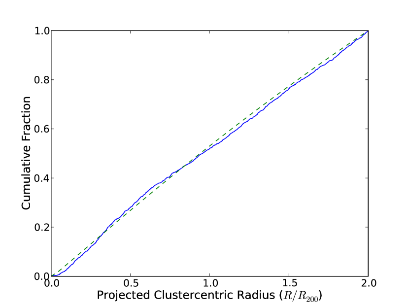
Figure 10.— Cumulative fraction of observed galaxies (within clusters with FOV complete to $2R_{200}$) as a function of projected clustercentric radius (solid blue line) compared to cumulative distribution of galaxies modeled by an NFW profile with c=2.6 and integrated out to a maximum radius of 10$R_{200}$ (dashed green line).

We now compare our results to the expected distribution of observed tidal features if the lifetime of the features is proportional to the local dynamical time and the generation of tidal features is independent of time or clustercentric radius (see Fig. 11). While the cumulative distribution of tidally-disturbed galaxies still lies below the model prediction within $R_{200}$, the deviation is still only statistically significant for the visually-selected sample of disturbed galaxies. For the sample complete within $R_{200}$, the K-S test shows that the visually-selected sample is drawn from a different distribution than the “all” sample with 95.8% confidence, the automated selection differs with 81.3% confidence, the intersection of the two samples is discrepant at 91.0% confidence, and the union is discrepant at 91.7%. For the sample complete to $2R_{200}$ none of the samples of disturbed galaxies are discrepant from the “all” sample at the $2\sigma$ level. These results are robust with reasonable changes in the concentration parameter used. If we instead use c=6, which is more accurate for the dark matter distribution for halos of this mass (Macció, Dutton, & van den Bosch, 2008), the K-S statistics are largely unchanged. Additionally, we tested a range of coefficients ($0.5-2.5t_{dyn}$) for the decay time behavior of tidal streams and, based on the one to two percent changes on the K-S probabilities, affirm that our conclusions are independent of modest changes to the choice of the coefficient. We find that this toy model, in which the lifetime of the features is proportional to the local dynamical time and the generation of tidal features is independent of time or clustercentric radius, qualitatively agrees with the observed deficit of tidal features at small clustercentric radii, but possibly would not solely account for the magnitude of the deficit within $\sim 0.5R_{200}$.

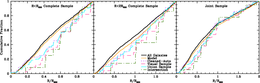
Figure 11.— Cumulative fraction of galaxies versus projected clustercentric radius. The left panel is the sample complete within $R_{200}$, the center panel is the sample complete within $2R_{200}$, and the right panel is the combination of the two samples (all galaxies within $R_{200}$ in clusters complete to $R_{200}$ and all galaxies within $2R_{200}$ in clusters complete to $2R_{200}$). Solid black line: “all” galaxies (dominated by undisturbed galaxies), dotted purple line: cleaned-auto sample, short-dashed red line: visually selected galaxies, long-dashed cyan line: union sample, dot-dashed green line: intersection sample, solid orange line: expected distribution for model (Eqn. 6) in which lifetime of the features is proportional to their dynamical time with a uniform incidence of features at all radii and an overall fraction of tidally disturbed galaxies set to match the observed value. All three panels show a deficit of tidally disturbed galaxies within $R_{200}$.

3.4. Local Density

When considering the effect of environment on cluster galaxies there is always a tension between the role of global vs. local environment. Part of the difficulty in addressing such issues is that the two measures of environment are correlated, and therefore large samples are needed to even begin to attempt to disentangle the two. A second difficulty is that local environment is inherently difficult to measure in clusters due to the complicated line-of-sight structure and relatively poor distance estimates. Here we make an attempt to study the dependence of tidal features on local density, but we face these same difficulties.

We quantify the local density using the standard measure of the projected distance to the 10th nearest galaxy with $M_{r}<-18$ that is also within the cluster’s red sequence in an attempt to mitigate contamination. We find no evidence that the rate of tidal features is dependent on local density as both the visual and the cleaned-auto samples differ from the full cluster sample at less than $2\sigma$ significance using a K-S test. We next attempt to remove the correlation between local density and clustercentric radius by dividing the galaxies into clustercentric annuli and within each annulus ranking galaxies uniformly by local density to range from 1 to 10 (10 being most dense). We then sum the density ranks of disturbed galaxies for all distance bins and compare that distribution to a random distribution (see Fig. 12). By doing this, we are asking whether at each radius the galaxies with tidal features are preferentially in environments of either low or high local density. We find that disturbed galaxies have no statistically significant deviations in ranks from a random distribution.

Although we find no evidence for local density having an effect on the incidence of tidal features, we caution that this is simply an absence of evidence rather than evidence of an absence, particularly because our measurement of local density is so crude.

Figure 12.— Histograms of galaxies versus ranked local density in radius annulus (a random distribution would be flat across all density bins). Top panel: visual sample of disturbed galaxies, 2nd panel down: cleaned-auto sample, 3rd panel down: union of visually and cleaned-auto-selected galaxies, bottom panel: intersection of visually and cleaned-auto-selected galaxies.

4. Conclusions

In a sample of 54 galaxy clusters $(0.04<z<0.15)$ containing 3551 early-type galaxies suitable for study, we identify those with tidal features both interactively and automatically. This constitutes the largest sample studied to date for signs of environmental dependence in the incidence of tidal features. We find tidal features in $\sim$ 3% of galaxies in this sample, with data of this particular depth. Regardless of the method used to classify tidal features, or the fidelity imposed on such classifications, we find a deficit of tidally disturbed galaxies with decreasing clustercentric radius that is most pronounced inside of $\sim 0.5R_{200}$.

Although this trend could be attributed to a rise in galaxy-galaxy interactions at large clustercentric distances, where the galaxy pair velocities might be better tuned to mergers, an alternative interpretation is that tidal features are preferentially erased at small clustercentric radii. We examine this hypothesis with a simple toy model that links tidal feature survival time to the local dynamical time and find that although qualitatively the effect is in the correct sense to explain the data, the model falls somewhat short quantitatively. Nevertheless, given the relative success and the limited statistics, we cannot exclude this model as a possible explanation for the radial trend in the incidence of tidal tails.

We also search for a dependence of the incidence of tidal features on local density and find no statistically significant evidence for such, even after accounting for the correlation between clustercentric radius and local density. Unfortunately, the large uncertainties in the measure of local environment limit the interpretation of a null result.

We demonstrate that interesting behavior exists in the rate of tidal features among cluster early-types as a function of clustercentric radius. This measure should provide some guidance for models of merging among early-types, which is conjectured to be significant in the build-up of the red sequence (Bell et al., 2004; Faber et al., 2007). Models of merging in and around clusters should aim to provide merger estimates based on observable features rather than theoretical constructs. We expect that such work will provide strong constraints on the effect of the cluster environment on the structure of galaxy halos, the build-up of the red sequence of galaxies, and the origin of the intracluster stellar population.

References

- Abraham et al. (1996) Abraham, R.G., Tanvir, N.R., Santiago, B.X., Ellis, R.S., Glazebrook, K., & van den Bergh, S. 1996, MNRAS, 279, 47L
- Barnes & Hernquist (1996) Barnes, J.E., & Hernquist, L. 1996, ApJ, 471, 115
- Bell et al. (2004) Bell, E.F., et al. 2004, ApJ, 608, 752
- Bertin & Arnouts (1996) Bertin, E., & Arnouts, S. 1996, Astronomy and Astrophysics Supplemental Series, 117, 393
- Bildfell et al. (2012) Bildfell, C. et al. 2012, MNRAS, accepted
- Bond et al. (1991) Bond, J.R., Cole, S., Efstathiou, G., & Kaiser, N. 1991, ApJ, 379, 440
- Boulade et al. (2003) Boulade, O., et al. 2003, SPIE, 4841, 72
- Bridge et al. (2010) Bridge, C.R., Carlberg, R.G., & Sullivan, M., 2010, ApJ, 709, 1067
- Budzynski et al. (2012) Budzynski, J.M., Koposov, S., McCarthy, I.G., McGee, S.L., & Belokurov V., 2012, MNRAS, 423, 104
- Carlberg, Pritchet, & Infante (1994) Carlberg, R.G., Pritchet, C.J., & Infante, L. 1994, ApJ, 435, 540
- Colbert et al. (2000) Colbert, J., Mulchaey, J., & Zabludoff, A. 2001, AJ, 121, 808
- Conselice et al. (2003) Conselice, C.J., Bershady, M.A., Dickinson, M., & Papovich, C. 2003, AJ, 126, 1183
- de Ravel et al. (2009) de Ravel, L., et al. 2009, A&A, 498, 379