Detailed analysis of prolate quadratures and interpolation formulas

Abstract

As demonstrated by Slepian et. al. in a sequence of classical papers (see [33], [34], [17], [35], [36]), prolate spheroidal wave functions (PSWFs) provide a natural and efficient tool for computing with bandlimited functions defined on an interval. As a result, PSWFs are becoming increasing popular in various areas in which such function occur - this includes physics (e.g. wave phenomena, fluid dynamics), engineering (e.g. signal processing, filter design), etc.

To use PSWFs as a computational tool, one needs fast and accurate numerical algorithms for the evaluation of PSWFs and related quantities, as well as for the construction of quadratures, interpolation formulas, etc. For the last half a century, substantial progress has been made in design of such algorithms - this includes both classical results (see e.g. [4]) as well as more recent developments (see e.g. [38]).

The complexity of many of the existing algorithms, however, is at least quadratic in the band limit $c$. For example, the evaluation of the $n$th eigenvalue of the prolate integral operator requires at least $O(c^{2})$ operations (see e.g. [38]); also, the construction of accurate quadrature rules for the integration of bandlimited functions of band limit $c$ requires $O(c^{3})$ operations (see e.g. [6]). Therefore, while the existing algorithms are quite satisfactory for moderate values of $c$ (e.g. $c\leq 10^{3}$), they tend to be relatively slow when $c$ is large (e.g. $c\geq 10^{4}$).

In this paper, we describe several numerical algorithms for the evaluation of PSWFs and related quantities, and design a class of PSWF-based quadratures for the integration of bandlimited functions. Also, we perform detailed analysis of the related properties of PSWFs. While the analysis is somewhat involved, the resulting numerical algorithms are quite simple and efficient in practice. For example, the evaluation of the $n$th eigenvalue of the prolate integral operator requires $O(n+c)$ operations; also, the construction of accurate quadrature rules for the integration of bandlimited functions of band limit $c$ requires $O(c)$ operations.

Our results are illustrated via several numerical experiments.

Keywords: bandlimited functions, prolate spheroidal wave functions, quadratures, interpolation

Math subject classification: 33E10, 34L15, 35S30, 42C10, 45C05, 54P05, 65D05, 65D15, 65D30, 65D32

1 Outline

1.1 Quadratures for Bandlimited Functions

The principal goal of this paper is a quadrature designed for the integration of bandlimited functions of a specified band limit $c>0$.

A function $f:\mathbb{R}\to\mathbb{R}$ is bandlimited of band limit $c>0$, if there exists a function $\sigma\in L^{2}\left[-1,1\right]$ such that

$$f(x)=\int_{-1}^{1}\sigma(t)\cdot e^{icxt}\;dt.$$ (1)

In other words, the Fourier transform of a bandlimited function is compactly supported. While (1) defines $f$ for all real $x$, one is often interested in bandlimited functions, whose argument is confined to an interval, e.g. $-1\leq x\leq 1$. Such functions are encountered in physics (wave phenomena, fluid dynamics), engineering (signal processing), etc. (see e.g. [33], [10], [29]).

By quadrature we mean a set of nodes

$$-1<t_{1}^{(n)}<\dots<t_{n}^{(n)}<1$$ (2)

and weights

$$W_{1}^{(n)},\dots,W_{n}^{(n)}.$$ (3)

If $f:(-1,1)\to\mathbb{R}$ is a bandlimited function, we use the quadrature to approximate the integral of $f$ over the interval $(-1,1)$ by a finite sum; more specifically,

$$\int_{-1}^{1}f(t)\;dt\approx\sum_{j=1}^{n}W_{j}^{(n)}f\left(t_{j}^{(n)}\right).$$ (4)

About half a century ago it was observed that the eigenfunctions of the integral operator $F_{c}:L^{2}\left[-1,1\right]\to L^{2}\left[-1,1\right]$, defined via the formula

$$F_{c}\left[\varphi\right](x)=\int_{-1}^{1}\varphi(t)e^{icxt}\;dt,$$ (5)

provide a natural tool for dealing with bandlimited functions, defined on the interval $\left[-1,1\right]$. Moreover, it was observed (see [34], [17], [35]) that the eigenfunctions of $F_{c}$ are precisely the prolate spheroidal wave functions (PSWFs) of band limit $c$, well known from the mathematical physics (see, for example, [24], [10]). Therefore, when designing a quadrature for the integration of bandlimited functions of band limit $c>0$, it is natural to require that this quadrature integrate several first PSWFs of band limit $c$ with high accuracy.

We formulate the principal objective of this paper in a more precise manner, as follows.

Principal goal of this paper.

Suppose that $c>0$ is a real number. For every integer $n>0$, we define a quadrature of order $n$ (for the integration of bandlimited functions of band limit $c$ over $(-1,1)$) by specifying $n$ nodes and $n$ weights (see (2), (3)). Suppose also that $\varepsilon>0$. We require that, for sufficiently large $n$, the quadrature of order $n$ integrate the first $n$ PSWFs of band limit $c$ up to the error $\varepsilon$. More specifically, we find the integer $M=M(c,\varepsilon)$ such that, for every integer $n\geq M$ and all integer $m=0,1,\dots,n-1$,

$$\left|\int_{-1}^{1}\psi_{m}(t)\;dt-\sum_{j=1}^{n}W_{j}^{(n)}\psi_{m}\left(t_{j}^{(n)}\right)\right|\leq\varepsilon,$$ (6)

where $\psi_{m}:(-1,1)\to\mathbb{R}$ is the $m$th PSWF of band limit $c$ (see Section 2.1).

Quadratures for the integration of bandlimited functions which satisfy (6) have already been discussed in the literature, for example:

Quadrature 1. Suppose that $n>0$ is an integer. The existence and uniqueness of $n$ nodes and weights, such that (6) holds for $\varepsilon=0$ and all $m=0,1,\dots,2n-1$, was first observed more than 100 years ago (see, for example, [15], [16], [21], [22]) for all Chebyshev systems, of which PSWFs are a special case (see [38]). Although numerical algorithms for the design of this optimal quadrature were recently constructed (see [6], [20], [39]), they tend to be rather expensive (require order $n^{3}$ operations with a large proportionality constant).

Quadrature 2. Another quadrature was suggested in [38]. The PSWF $\psi_{n}$ has $n$ roots $t_{1},\dots,t_{n}$ in the interval $(-1,1)$ (see Theorem 1 in Section 2.1); the idea is to use these roots as the quadrature nodes, solve the linear system of $n$ equations

$$\left\{\sum_{j=1}^{n}\psi_{m}(t_{j})W_{j}=\int_{-1}^{1}\psi_{m}(t)\;dt\right\}_{m=0}^{n-1}$$ (7)

for the unknowns $W_{1},\dots,W_{n}$, and use the resulting weights and nodes to define a quadrature for the integration of functions of band limit $2c$. This approach is justified by the generalization of the Euclid’s division algorithm for PSWFs (see [38]), and is less expensive computationally than the previous one (its cost is dominated by the cost of solving the linear system (7)). The same quadrature can be used to integrate functions of band limit $c$, since (7) implies that (6) holds with $\varepsilon=0$, for all $m=0,\dots,n-1$.

In this paper, we describe another quadrature whose nodes are the $n$ roots of $\psi_{n}$ in $\left(-1,1\right)$. However, its weights differ from the solution of (7), and can be evaluated in $O(n)$ operations (see Section 4.4 and Section 5 below).

Thus, the quadratures of this paper are much faster to evaluate than those described above. Moreover, (6) ensures that their accuracy is similar to that of Quadrature 2. Also, their nodes and weights can be used as starting points for the scheme that computes the optimal Quadrature 1.

In order to define the weights, to make sure that (6) holds and to be able to compute them efficiently, we need to analyze the PSWFs in a somewhat detailed manner. This analysis will be preceded by a heuristic explanation, which provides some intuition as well as prevents one from the danger of not seeing the forest for the trees (see Section 1.2 below). Section 1.3 contains a short overview of the analysis. Section 2 contains mathematical and numerical preliminaries, to be used in the rest of the paper. In Section 3, we summarize the principal analytical results of the paper. Section 4 contains the corresponding theorems and proofs. Section 5 contains the description and analysis of the numerical algorithms for the evaluation of the quadrature and some related quantities. In Section 6, we report the results of several numerical experiments.

1.2 Intuition Behind Quadrature Weights

We recall the following classical interpolation problem. Suppose that $t_{1},\dots,t_{n}$ are $n$ distinct points in the interval $(-1,1)$. We need to find the real numbers $W_{1},\dots,W_{n}$ such that

$$\int_{-1}^{1}p(t)\;dt=\sum_{i=1}^{n}W_{i}\cdot p(t_{i}),$$ (8)

for all the polynomials $p$ of degree at most $n-1$. In other words, the quadrature with nodes $t_{1},\dots,t_{n}$ and weights $W_{1},\dots,W_{n}$ integrates all the polynomials of degree up to $n-1$ exactly (see (2), (3), (4)).

To solve the problem, one constructs $n$ polynomials $l_{1},\dots,l_{n}$ of degree $n-1$ with the property

$$\l_{j}(t_{i})=\begin{cases}0&i\neq j,\\ 1&i=j\end{cases}$$ (9)

for every integer $i,j=1,\dots,n$ (see, for example,[14]). It is easy to verify that, for every $j=1,\dots,n$, the polynomial $l_{j}$ is defined via the formula

$$l_{j}(t)=\frac{w_{n}(t)}{w_{n}^{\prime}(t_{j})\cdot(t-t_{j})},$$ (10)

where $w_{n}$ is the polynomial of degree $n$ whose roots are precisely $t_{1},\dots,t_{n}$. The weights $W_{1},\dots,W_{n}$ are defined via the formula

$$W_{j}=\int_{-1}^{1}l_{j}(t)\;dt=\frac{1}{w_{n}^{\prime}(t_{j})}\int_{-1}^{1}\frac{w_{n}(t)\;dt}{t-t_{j}},$$ (11)

for every integer $j=1,\dots,n$. We observe that a single function $w_{n}$ is used to define all the $n$ weights; also, $w_{n}$ is a polynomial of degree $n$, and hence does not belong to the space of the polynomials of degree up to $n-1$.

In our case, the basis functions are the PSWFs and not the polynomials. Suppose that the roots $t_{1},\dots,t_{n}$ of $\psi_{n}$ in the interval $(-1,1)$ are chosen to be the nodes of the quadrature. If we choose the weights $W_{1},\dots,W_{n}$ such that the resulting quadrature integrates the first $n$ PSWFs exactly, this will lead to the linear system (7), and hence to Quadrature 2 from Section 1.1. Instead, we define the weights via using $\psi_{n}$ in the same way we used $w_{n}$ in (11). More specifically, similar to (10), for every integer $j=1,\dots,n$, we define the function $\varphi_{j}:(-1,1)\to\mathbb{R}$ via the formula

$$\varphi_{j}(t)=\frac{\psi_{n}(t)}{\psi_{n}^{\prime}(t_{j})\cdot(t-t_{j})}.$$ (12)

We observe that, for every integer $i,j=1,\dots,n$,

$$\varphi_{j}(t_{i})=\begin{cases}0&i\neq j,\\ 1&i=j,\end{cases}$$ (13)

analogous to (9). Viewed as a function on the whole real line, each $\varphi_{j}$ is bandlimited with the same band limit $c$ (see, for example, Theorem 59 in Section 4.4.1 or Theorem 19.3 in [31]). On the other hand, $\varphi_{j}$ does not belong to the span of $\psi_{0},\psi_{1},\dots,\psi_{n-1}$ (see Theorem 59 in Section 4.4.1). We define the weights $W_{1},\dots,W_{n}$ via the formula

$$W_{j}=\int_{-1}^{1}\varphi_{j}(t)\;dt,$$ (14)

for $j=1,2,\dots,n$. The weights $W_{1},\dots,W_{n}$, defined via (14), are different from the solution of the linear system (7). Nevertheless, the resulting quadrature is expected to satisfy (6) with $\varepsilon$ of order $|\lambda_{n}|$ (see Theorem 60 in Section 4.4.2), since the reciprocal of $\psi_{n}$ can be approximated well by a rational function with $n$ poles. Making the latter statement precise is the principal purpose of Section 4 of this paper. While the analysis of the issue is somewhat detailed, the principal idea is simple enough to be presented in the next few sentences.

If $P$ is a polynomial with $m$ simple roots $z_{1},\dots,z_{m}$ in $(-1,1)$, then the function $z\to P(z)^{-1}$ is meromorphic in the complex plane; moreover,

$$\frac{1}{P(z)}=\sum_{j=1}^{m}\frac{1}{P^{\prime}(z_{j})\cdot(z-z_{j})},$$ (15)

for all complex $z$ different from $z_{1},\dots,z_{m}$ (see Theorem 27 in Section 2.8). The right-hand side of (15) is referred to as “partial fractions expansion of $P^{-1}$”. Similarly, the function $z\to\psi_{n}(z)^{-1}$ is meromorphic; however, it has infinitely many poles, all of which are real and simple (see Corollary 3 in Section 4.1.1), and exactly $n$ of which lie in $(-1,1)$ (see Theorem 1 in Section 2.1). Suppose that the roots of $\psi_{n}$ in $(-1,1)$ are denoted by $t_{1}<\dots<t_{n}$. Motivated by (15), we analyze the partial fractions expansion of $\psi_{n}^{-1}$. It turns out that

$$\frac{1}{\psi_{n}(t)}=\sum_{j=1}^{n}\frac{1}{\psi_{n}^{\prime}(t_{j})\cdot(t-t_{j})}+O(|\lambda_{n}|),$$ (16)

for real $-1<t<1$ (see Section 4.3 and Theorem 27 in Section 2.8). In other words, (16) means that the reciprocal of $\psi_{n}$ differs from a certain rational function with $n$ poles by a function, whose magnitude in the interval $(-1,1)$ is of order $|\lambda_{n}|$.

A rigorous version of (16) is established and proven in Section 4.3. The relation between (6), (12), (14) and (16) is studied in Section 4.4. The results of these two sections rely on the machinery, developed in Sections 4.1, 4.2.

1.3 Overview of the Analysis

1.3.1 Partial Fractions Expansion of $1/\psi_{n}$

To establish (16), we proceed as follows. Suppose that $x_{1}<x_{2}<\dots$ are the roots of $\psi_{n}$ in $(1,\infty)$ (see Corollary 3 in Section 4.1.1). Suppose also that $M>1$, and $R>1$ is a point between $x_{M}$ and $x_{M+1}$. In other words,

$$1<x_{1}<x_{2}<\dots<x_{M}<R<x_{M+1}<\dots.$$ (17)

Then, for all real $-1<t<1$,

$$\frac{1}{\psi_{n}(t)}-\sum_{j=1}^{n}\frac{1}{\psi_{n}^{\prime}(t_{j})\cdot(t-t_{j})}=$$

$$\sum_{k=1}^{M}\left(\frac{1}{\psi_{n}^{\prime}(x_{k})\cdot(t-x_{k})}+\frac{1}{\psi_{n}^{\prime}(-x_{k})\cdot(t+x_{k})}\right)+\frac{1}{2\pi i}\oint_{\Gamma_{R}}\frac{dz}{\psi_{n}(z)\cdot(z-t)},$$ (18)

where $\Gamma_{R}$ is the boundary of the square $\left[-R,R\right]\times\left[-iR,iR\right]$, traversed in the counterclockwise direction (see Theorem 27 in Section 2.8).

Suppose now that $x>1$ is a root of $\psi_{n}$. We observe that $\psi_{n}$ is a holomorphic function defined in the entire complex plane. We use the integral equation (37) in Section 2.1 and Theorem 25 in Section 2.8 to show that

$$\sqrt{|\psi_{n}(x+it)|^{2}+|\psi_{n}^{\prime}(x+it)|^{2}\cdot\frac{|(x+it)^{2}-1|}{|c^{2}\cdot(x+it)^{2}-\chi_{n}|}}\sim$$

$$\frac{e^{ct}\cdot|\psi_{n}(1)|\cdot\sqrt{2}}{ct\cdot|\lambda_{n}|},\quad t\to\infty$$ (19)

(see Theorem 36 in Section 4.2.2). On the other hand, we use the differential equation (48) in Section 2.1 and Theorem 22 in Section 2.5 to show that

$$\sqrt{|\psi_{n}(x+it)|^{2}+|\psi_{n}^{\prime}(x+it)|^{2}\cdot\frac{|(x+it)^{2}-1|}{|c^{2}\cdot(x+it)^{2}-\chi_{n}|}}\leq$$

$$\frac{e^{1/4}\cdot e^{ct}\cdot|\psi_{n}^{\prime}(x)|\cdot(x^{2}-1)^{3/4}}{ct\cdot\left(x^{2}-(\chi_{n}/c^{2})\right)^{1/4}}$$ (20)

(see Theorems 37, 38, 39, 40, 42 in Section 4.2.2). We combine (19) and (20) to establish the inequality

$$\frac{1}{\left|\psi_{n}^{\prime}(x)\right|}\leq e^{1/4}\cdot\left|\lambda_{n}\right|\cdot\frac{(x^{2}-1)^{\frac{3}{4}}}{(x^{2}-(\chi_{n}/c^{2}))^{\frac{1}{4}}}$$ (21)

(see Theorem 43 in Section 4.2.2). Then, we use (21) to show that, for every integer $M>1$,

$$\left|\sum_{k=1}^{M}\frac{1}{(t-x_{k})\cdot\psi_{n}^{\prime}(x_{k})}\right|<5\cdot|\lambda_{n}|\cdot\left(\log(2\cdot x_{M})+(\chi_{n})^{1/4}\right)$$ (22)

(see Theorems 44, 45 in Section 4.3.1 for a more precise statement).

We observe that (22) provides an upper bound on the first summand in right-hand side of (18). While this bound is of order $|\lambda_{n}|$ for $x_{M}<O(|\lambda_{n}|^{-1})$, it diverges if we let $M$ go to infinity (see, however, (24) below).

To overcome this obstacle, we use the integral equation (44) in Section 2.1 to analyze the behavior of $\psi_{n}(x)$ and $\psi_{n}^{\prime}(x)$ for $x>|\lambda_{n}|^{-2}$ (see Section 4.3.2). In particular, if $x>1$ is a root of $\psi_{n}$ and if $x>|\lambda_{n}|^{-2}$, then

$$\left|\psi_{n}^{\prime}(x)\right|=\left|\frac{2\psi_{n}(1)}{\lambda_{n}x}\right|\cdot\left[1+O\left(\left|x\cdot\lambda_{n}\right|^{-1}\right)\right]$$ (23)

(see Theorem 51 in Section 4.3.2 for a more precise statement). More detailed analysis reveals that, if $y>x>|\lambda_{n}|^{-2}$ are two consecutive roots of $\psi_{n}$ and $-1<t<1$ is a real number, then

$$\left|\frac{1}{\psi_{n}^{\prime}(x)\cdot(x-t)}+\frac{1}{\psi_{n}^{\prime}(y)\cdot(y-t)}\right|\leq 20\cdot c\cdot\int_{x}^{y}\frac{ds}{s^{2}}$$ (24)

(see Theorem 52 in Section 4.3.2).

In Theorem 53 of Section 4.3.3, we establish, for all real $-1<t<1$, the inequality of the form

$$\left|\sum_{k=1}^{\infty}\frac{1}{\psi_{n}^{\prime}(x_{k})\cdot(x_{k}-t)}\right|\leq\text{const}\cdot|\lambda_{n}|\cdot\left(\log\left(\frac{1}{|\lambda_{n}|}\right)+(\chi_{n})^{1/4}\right),$$ (25)

where (22), (24) are used to bound the head and the tail of the infinite sum, respectively.

Eventually, we analyze the behavior of $\psi_{n}$ of the complex argument to demonstrate that, for all real $-1<t<1$,

$$\limsup_{k\to\infty}\left|\frac{1}{2\pi i}\oint_{\Gamma_{R_{k}}}\frac{dz}{\psi_{n}(z)\cdot(z-t)}\right|<2\sqrt{2}\cdot|\lambda_{n}|,$$ (26)

where $\left\{R_{k}\right\}$ is a certain sequence that tends to infinity, and the contours $\Gamma_{R_{k}}$ are as in (18) (see Theorems 54, 55 in Section 4.3.3 for more details). We substitute (25) and (26) into (18) to obtain, for all real $-1<t<1$, an inequality of the form

$$\left|\frac{1}{\psi_{n}(t)}-\sum_{j=1}^{n}\frac{1}{\psi_{n}^{\prime}(t_{j})\cdot(t-t_{j})}\right|\leq\text{const}\cdot|\lambda_{n}|\cdot\left(\log\left(\frac{1}{|\lambda_{n}|}\right)+(\chi_{n})^{1/4}\right)$$ (27)

(see Theorems 56, 58 in Section 4.3.3). In the next subsection, we overview the implications of (27) to the analysis of the quadrature, discussed in Section 1.2.

1.3.2 Quadrature Weights

Roughly speaking, (27) asserts that, for all real $-1<t<1$,

$$\frac{1}{\psi_{n}(t)}-\sum_{j=1}^{n}\frac{1}{\psi_{n}^{\prime}(t_{j})\cdot(t-t_{j})}=O\left(|\lambda_{n}|\right).$$ (28)

In other words, the left-hand side of (28) is uniformly bounded in $(-1,1)$, and its magnitude is of order $|\lambda_{n}|$. If we multiply both sides of (28) by $\psi_{n}(t)$ and use (12), we obtain

$$1=\varphi_{1}(t)+\dots+\varphi_{n}(t)+\psi_{n}(t)\cdot O\left(|\lambda_{n}|\right)$$ (29)

In other words, $\varphi_{1},\dots,\varphi_{n}$ constitute a partition of unity in the interval $(-1,1)$, up to an error of order $|\lambda_{n}|$. We integrate both sides of (29) over $(-1,1)$ and use Theorem 1 in Section 2.1 and (14) in Section 1.2 to obtain

$$2=W_{1}+\dots+W_{n}+O\left(|\lambda_{n}|\right)$$ (30)

(see Section 4.4.4 for more details).

Suppose now that $m\neq n$ is an integer. We multiply both sides of (29) by $\psi_{m}$ to obtain

$$\psi_{m}(t)=\sum_{j=1}^{n}\psi_{m}(t)\cdot\varphi_{j}(t)+\psi_{m}(t)\cdot\psi_{n}(t)\cdot O\left(|\lambda_{n}|\right).$$ (31)

On the other hand, for every integer $j=1,\dots,n$, we use integration by parts to evaluate

$$\int_{-1}^{1}\varphi_{j}(t)\cdot\psi_{m}(t)\;dt=$$

$$\frac{|\lambda_{m}|^{2}\cdot\psi_{m}(t_{j})}{|\lambda_{m}|^{2}-|\lambda_{n}|^{2}}\cdot\left[W_{j}+\frac{ic\lambda_{n}}{\psi_{n}^{\prime}(t_{j})}\int_{0}^{1}\psi_{n}(x)\cdot e^{-icxt_{j}}\;dx\right]$$ (32)

(see Theorem 59 in Section 4.4.1). We combine (27), (31) and (32) with some additional analysis to conclude that, for all integer $0\leq m<n$,

$$\left|\int_{-1}^{1}\psi_{m}(t)\;dt-\sum_{j=1}^{n}\psi_{m}(t_{j})\cdot W_{j}\right|\leq\text{const}\cdot|\lambda_{n}|\cdot\left(\log\frac{1}{|\lambda_{n}|}+\chi_{n}\right)$$ (33)

(see Theorems 60, 62 in Section 4.4.2).

According to (33), the quadrature error (6) in Section 1.1 is roughly of order $|\lambda_{n}|$. It remains to establish for what values of $n$ this error is smaller than the predefined accuracy parameter $\varepsilon>0$. In Section 4.4.3, we combine Theorems 6, 7, 11 with (33) to achieve that goal. Namely, we show that, if

$$n>\frac{2c}{\pi}+\text{const}\cdot\log(c)\cdot\left(\log(c)+\log\frac{1}{\varepsilon}\right),$$ (34)

then

$$\left|\int_{-1}^{1}\psi_{m}(t)\;dt-\sum_{j=1}^{n}\psi_{m}(t_{j})\cdot W_{j}\right|\leq\varepsilon,$$ (35)

for all integer $0\leq m<n$ (see Theorem 65).

Numerical experiments seem to indicate that the situation is even better in practice: namely, to achieve the desired accuracy it suffices to pick the minimal $n$ such that $\left|\lambda_{n}\right|<\varepsilon$, which occurs for $n=2c/\pi+O((\log c)\cdot(-\log\varepsilon))$ (see Section 6, in particular, Conjecture 2 and Experiment 14 in Section 6.2.1).

2 Mathematical and Numerical Preliminaries

In this section, we introduce notation and summarize several facts to be used in the rest of the paper.

2.1 Prolate Spheroidal Wave Functions

In this subsection, we summarize several facts about the PSWFs. Unless stated otherwise, all these facts can be found in [38], [30], [18], [34], [17], [25], [26].

Given a real number $c>0$, we define the operator $F_{c}:L^{2}\left[-1,1\right]\to L^{2}\left[-1,1\right]$ via the formula

$$F_{c}\left[\varphi\right](x)=\int_{-1}^{1}\varphi(t)e^{icxt}\;dt.$$ (36)

Obviously, $F_{c}$ is compact. We denote its eigenvalues by $\lambda_{0},\lambda_{1},\dots,\lambda_{n},\dots$ and assume that they are ordered such that $\left|\lambda_{n}\right|\geq\left|\lambda_{n+1}\right|$ for all natural $n\geq 0$. We denote by $\psi_{n}$ the eigenfunction corresponding to $\lambda_{n}$. In other words, the following identity holds for all integer $n\geq 0$ and all real $-1\leq x\leq 1$:

$$\lambda_{n}\psi_{n}\left(x\right)=\int_{-1}^{1}\psi_{n}(t)e^{icxt}\;dt.$$ (37)

We adopt the convention that $\|\psi_{n}\|_{L^{2}\left[-1,1\right]}=1$. The following theorem describes the eigenvalues and eigenfunctions of $F_{c}$.

Theorem 1.

Suppose that $c>0$ is a real number, and that the operator $F_{c}$ is defined via (36) above. Then, the eigenfunctions $\psi_{0},\psi_{1},\dots$ of $F_{c}$ are purely real, are orthonormal and are complete in $L^{2}\left[-1,1\right]$. The even-numbered functions are even, the odd-numbered ones are odd. Each function $\psi_{n}$ has exactly $n$ simple roots in $\left(-1,1\right)$. All eigenvalues $\lambda_{n}$ of $F_{c}$ are non-zero and simple; the even-numbered ones are purely real and the odd-numbered ones are purely imaginary; in particular, $\lambda_{n}=i^{n}\left|\lambda_{n}\right|$.

We define the self-adjoint operator $Q_{c}:L^{2}\left[-1,1\right]\to L^{2}\left[-1,1\right]$ via the formula

$$Q_{c}\left[\varphi\right](x)=\frac{1}{\pi}\int_{-1}^{1}\frac{\sin\left(c\left(x-t\right)\right)}{x-t}\;\varphi(t)\;dt.$$ (38)

Clearly, if we denote by $\mathcal{F}:L^{2}(\mathbb{R})\to L^{2}(\mathbb{R})$ the unitary Fourier transform, then

$$Q_{c}\left[\varphi\right](x)=\chi_{\left[-1,1\right]}(x)\cdot\mathcal{F}^{-1}\left[\chi_{\left[-c,c\right]}(\xi)\cdot\mathcal{F}\left[\varphi\right](\xi)\right](x),$$ (39)

where $\chi_{\left[-a,a\right]}:\mathbb{R}\to\mathbb{R}$ is the characteristic function of the interval $\left[-a,a\right]$, defined via the formula

$$\chi_{\left[-a,a\right]}(x)=\begin{cases}1&-a\leq x\leq a,\\ 0&\text{otherwise},\end{cases}$$ (40)

for all real $x$. In other words, $Q_{c}$ represents low-passing followed by time-limiting. $Q_{c}$ relates to $F_{c}$, defined via (36), by

$$Q_{c}=\frac{c}{2\pi}\cdot F_{c}^{\ast}\cdot F_{c},$$ (41)

and the eigenvalues $\mu_{n}$ of $Q_{n}$ satisfy the identity

$$\mu_{n}=\frac{c}{2\pi}\cdot\left|\lambda_{n}\right|^{2},$$ (42)

for all integer $n\geq 0$. Obviously,

$$\mu_{n}<1,$$ (43)

for all integer $n\geq 0$, due to (39). Moreover, $Q_{c}$ has the same eigenfunctions $\psi_{n}$ as $F_{c}$. In other words,

$$\mu_{n}\psi_{n}(x)=\frac{1}{\pi}\int_{-1}^{1}\frac{\sin\left(c\left(x-t\right)\right)}{x-t}\;\psi_{n}(t)\;dt,$$ (44)

for all integer $n\geq 0$ and all $-1\leq x\leq 1$. Also, $Q_{c}$ is closely related to the operator $P_{c}:L^{2}(\mathbb{R})\to L^{2}(\mathbb{R})$, defined via the formula

$$P_{c}\left[\varphi\right](x)=\frac{1}{\pi}\int_{-\infty}^{\infty}\frac{\sin\left(c\left(x-t\right)\right)}{x-t}\;\varphi(t)\;dt,$$ (45)

which is a widely known orthogonal projection onto the space of functions of band limit $c>0$ on the real line $\mathbb{R}$.

The following theorem about the eigenvalues $\mu_{n}$ of the operator $Q_{c}$, defined via (38), can be traced back to [18]:

Theorem 2.

Suppose that $c>0$ and $0<\alpha<1$ are positive real numbers, and that the operator $Q_{c}:L^{2}\left[-1,1\right]\to L^{2}\left[-1,1\right]$ is defined via (38) above. Suppose also that the integer $N(c,\alpha)$ is the number of the eigenvalues $\mu_{n}$ of $Q_{c}$ that are greater than $\alpha$. In other words,

$$N(c,\alpha)=\max\left\{k=1,2,\dots\;:\;\mu_{k-1}>\alpha\right\}.$$ (46)

Then,

$$N(c,\alpha)=\frac{2c}{\pi}+\left(\frac{1}{\pi^{2}}\log\frac{1-\alpha}{\alpha}\right)\log c+O\left(\log c\right).$$ (47)

According to (47), there are about $2c/\pi$ eigenvalues whose absolute value is close to one, order of $\log c$ eigenvalues that decay exponentially, and the rest of them are very close to zero.

The eigenfunctions $\psi_{n}$ of $Q_{c}$ turn out to be the PSWFs, well known from classical mathematical physics [24]. The following theorem, proved in a more general form in [35], formalizes this statement.

Theorem 3.

For any $c>0$, there exists a strictly increasing unbounded sequence of positive numbers $\chi_{0}<\chi_{1}<\dots$ such that, for each integer $n\geq 0$, the differential equation

$$\left(1-x^{2}\right)\psi^{\prime\prime}(x)-2x\cdot\psi^{\prime}(x)+\left(\chi_{n}-c^{2}x^{2}\right)\psi(x)=0$$ (48)

has a solution that is continuous on $\left[-1,1\right]$. Moreover, all such solutions are constant multiples of the eigenfunction $\psi_{n}$ of $F_{c}$, defined via (36) above.

Remark 1.

For all real $c>0$ and all integer $n\geq 0$, (37) defines an analytic continuation of $\psi_{n}$ onto the entire complex plane. All the roots of $\psi_{n}$ are simple and real. In addition, the ODE (48) is satisfied for all complex $x$.

Many properties of the PSWF $\psi_{n}$ depend on whether the eigenvalue $\chi_{n}$ of the ODE (48) is greater than or less than $c^{2}$. In the following theorem from [25], [26], we describe a simple relationship between $c,n$ and $\chi_{n}$.

Theorem 4.

Suppose that $n\geq 2$ is a non-negative integer.

• If $n\leq(2c/\pi)-1$, then $\chi_{n}<c^{2}$.

• If $n\geq(2c/\pi)$, then $\chi_{n}>c^{2}$.

• If $(2c/\pi)-1<n<(2c/\pi)$, then either inequality is possible.

In the following theorem, upper and lower bounds on $\chi_{n}$ in terms of $c$ and $n$ are provided.

Theorem 5.

Suppose that $c>0$ is a real number, and $n\geq 0$ is an integer. Then,

$$n\left(n+1\right)<\chi_{n}<n\left(n+1\right)+c^{2}.$$ (49)

It turns out that, for the purposes of this paper, the inequality (49) is insufficiently sharp. More accurate bounds on $\chi_{n}$ are described in the following three theorems (see [25], [26], [27], [28]).

Theorem 6.

Suppose that $n\geq 2$ is a positive integer, and that $\chi_{n}>c^{2}$. Then,

$$n< \;\frac{2}{\pi}\int_{0}^{1}\sqrt{\frac{\chi_{n}-c^{2}t^{2}}{1-t^{2}}}\;dt=$$

$$\;\frac{2}{\pi}\sqrt{\chi_{n}}\cdot E\left(\frac{c}{\sqrt{\chi_{n}}}\right)<n+3,$$ (50)

where the function $E:\left[0,1\right]\to\mathbb{R}$ is defined via (109) in Section 2.3.

Theorem 7.

Suppose that $n$ is a positive integer, and that

$$n>\frac{2c}{\pi}+\frac{2}{\pi^{2}}\cdot\delta\cdot\log\left(\frac{4e\pi c}{\delta}\right),$$ (51)

for some

$$0<\delta<\frac{5\pi}{4}\cdot c.$$ (52)

Then,

$$\chi_{n}>c^{2}+\frac{4}{\pi}\cdot\delta\cdot c.$$ (53)

Theorem 8.

Suppose that $n$ is a positive integer, and that

$$\frac{2c}{\pi}\leq n\leq\frac{2c}{\pi}+\frac{2}{\pi^{2}}\cdot\delta\cdot\log\left(\frac{4e\pi c}{\delta}\right)-3,$$ (54)

for some

$$3<\delta<\frac{5\pi}{4}\cdot c.$$ (55)

Then,

$$\chi_{n}<c^{2}+\frac{8}{\pi}\cdot\delta\cdot c.$$ (56)

The following theorem is a direct consequence of Theorem 6.

Theorem 9.

Suppose that $n>0$ is a positive integer, and that

$$n>\frac{2c}{\pi}+1.$$ (57)

Then,

$$\chi_{n}>c^{2}+1.$$ (58)

Proof.

It follows from (50) of Theorem 6 that

$$n \;<\frac{2c}{\pi}\int_{0}^{1}\sqrt{1+\frac{\chi_{n}-c^{2}}{c^{2}}\cdot\frac{1}{1-t^{2}}}\;dt$$

$$\;<\frac{2c}{\pi}+\frac{2}{\pi}\cdot\sqrt{\chi_{n}-c^{2}}\cdot\int_{0}^{1}\frac{dt}{\sqrt{1-t^{2}}}=\frac{2c}{\pi}+\sqrt{\chi_{n}-c^{2}}.$$ (59)

We combine (59) with (57) to obtain (58). ∎

In the following theorem from [27], [28], we provide an upper bound on $|\lambda_{n}|$ in terms of $n$ and $c$.

Theorem 10.

Suppose that $c>0$ is a real number, and that

$$c>22.$$ (60)

Suppose also that $\delta>0$ is a real number, and that

$$3<\delta<\frac{\pi c}{16}.$$ (61)

Suppose, in addition, that $n$ is a positive integer, and that

$$n>\frac{2c}{\pi}+\frac{2}{\pi^{2}}\cdot\delta\cdot\log\left(\frac{4e\pi c}{\delta}\right).$$ (62)

Suppose furthermore that the real number $\xi(n,c)$ is defined via the formula

$$\xi(n,c)=7056\cdot c\cdot\exp\left[-\delta\left(1-\frac{\delta}{2\pi c}\right)\right].$$ (63)

Then,

$$\left|\lambda_{n}\right|<\xi(n,c).$$ (64)

In the following theorem from [27], [28], we provide another upper bound on $|\lambda_{n}|$.

Theorem 11.

Suppose that $n>0$ is a positive integer, and that

$$n>\frac{2c}{\pi}+\sqrt{42}.$$ (65)

Suppose also that the real number $x_{n}$ is defined via the formula

$$x_{n}=\frac{\chi_{n}}{c^{2}}.$$ (66)

Then,

$$|\lambda_{n}|<$$

$$1195\cdot c\cdot(x_{n})^{\frac{3}{4}}\cdot(x_{n}-1)^{\frac{1}{4}}\cdot\left(x_{n}-\frac{1}{2}\right)^{3}\cdot\exp\left[-\frac{\pi}{4}\cdot\left(\sqrt{x_{n}}-\frac{1}{\sqrt{x_{n}}}\right)\cdot c\right].$$ (67)

The following theorem is a combination of certain results from [30] and [25], [26].

Theorem 12.

Suppose that $c>0$ is a real number, and that $\chi_{n}>c^{2}$. Then,

$$\frac{1}{2}<\psi_{n}^{2}(1)<n+\frac{1}{2}.$$ (68)

The following theorem appears in [25], [26].

Theorem 13.

Suppose that $n\geq 0$ is a non-negative integer, and that $x,y$ are two arbitrary extremum points of $\psi_{n}$ in $(-1,1)$. If $\left|x\right|<\left|y\right|$, then

$$\left|\psi_{n}(x)\right|<\left|\psi_{n}(y)\right|.$$ (69)

If, in addition, $\chi_{n}>c^{2}$, then

$$\left|\psi_{n}(x)\right|<\left|\psi_{n}(y)\right|<\left|\psi_{n}(1)\right|.$$ (70)

The following theorem appears in [32].

Theorem 14.

For all real $c>0$ and all natural $n\geq 1$,

$$\max_{m\leq n+1}\;\max_{\left|t\right|\leq 1}|\psi_{m}(t)|\leq 2\sqrt{n}.$$ (71)

In the following theorem, we provide a recurrence relation between the derivatives of $\psi_{n}$ of arbitrary order (see Lemma 9.1 in [38]).

Theorem 15.

Suppose that $c>0$ is a real number, and that $n\geq 0$ is an integer. Then,

$$\left(1-t^{2}\right)\psi_{n}^{\prime\prime\prime}(t)-4t\psi_{n}^{\prime\prime}(t)+\left(\chi_{n}-c^{2}t^{2}-2\right)\psi_{n}^{\prime}(t)-2c^{2}t\psi_{n}(t)=0$$ (72)

for all real $t$. Moreover, for all integer $k\geq 2$ and all real $t$,

$$\left(1-t^{2}\right)\psi_{n}^{(k+2)}(t)-2\left(k+1\right)t\psi_{n}^{(k+1)}(t)+\left(\chi_{n}-k\left(k+1\right)-c^{2}t^{2}\right)\psi_{n}^{(k)}(t)$$

$$\quad\quad-c^{2}kt\psi_{n}^{(k-1)}(t)-c^{2}k\left(k-1\right)\psi_{n}^{(k-2)}(t)=0.$$ (73)

We refer to the roots of $\psi_{n}$, the roots of $\psi_{n}^{\prime}$ and the turning points of the ODE (48) as ”special points”. In the following theorem from [25], [26], we describe the location of some of the special points.

Theorem 16 (Special points).

Suppose that $n\geq 2$ is a positive integer. Suppose also that $t_{1}<t_{2}<\dots$ are the roots of $\psi_{n}$ in $(-1,1)$, and that $s_{1}<s_{2}<\dots$ are the roots of $\psi_{n}^{\prime}$ in $(-1,1)$. If $\chi_{n}<c^{2}$, then

$$-1<-\frac{\sqrt{\chi_{n}}}{c}<s_{1}<t_{1}<s_{2}<\dots<t_{n-1}<s_{n}<t_{n}<s_{n+1}<\frac{\sqrt{\chi_{n}}}{c}<1$$ (74)

In particular, $\psi_{n}$ has $n$ roots in $(-1,1)$, and $\psi_{n}^{\prime}$ has $n+1$ roots in $(-1,1)$. On the other hand, if $\chi_{n}>c^{2}$, then

$$-\frac{\sqrt{\chi_{n}}}{c}<-1<t_{1}<s_{1}<t_{2}<\dots<t_{n-1}<s_{n-1}<t_{n}<1<\frac{\sqrt{\chi_{n}}}{c}.$$ (75)

In particular, $\psi_{n}$ has $n$ roots in $(-1,1)$, and $\psi_{n}^{\prime}$ has $n-1$ roots in $(-1,1)$.

In the following theorem, proven in [25], [26], we describe a relation between the magnitude of $\psi_{n}$ and $\psi_{n}^{\prime}$ in the interval $(-1,1)$.

Theorem 17.

Suppose that $n\geq 0$ is a non-negative integer, and that the functions $p,q:\mathbb{R}\to\mathbb{R}$ are defined via (140) in Section 2.6. Suppose also that the functions $Q,\tilde{Q}:(0,\min\left\{\sqrt{\chi_{n}}/c,1\right\})\to\mathbb{R}$ are defined, respectively, via the formulae

$$Q(t) \;=\psi_{n}^{2}(t)+\frac{p(t)}{q(t)}\cdot\left(\psi^{\prime}_{n}(t)\right)^{2}=\psi_{n}^{2}(t)+\frac{\left(1-t^{2}\right)\cdot\left(\psi^{\prime}_{n}(t)\right)^{2}}{\chi_{n}-c^{2}t^{2}}$$ (76)

and

$$\tilde{Q}(t) \;=p(t)\cdot q(t)\cdot Q(t)$$

$$\;=\left(1-t^{2}\right)\cdot\left(\left(\chi_{n}-c^{2}t^{2}\right)\cdot\psi_{n}^{2}(t)+\left(1-t^{2}\right)\cdot\left(\psi^{\prime}_{n}(t)\right)^{2}\right).$$ (77)

Then, $Q$ is increasing in the interval $\left(0,\min\left\{\sqrt{\chi_{n}}/c,1\right\}\right)$, and $\tilde{Q}$ is decreasing in the interval $\left(0,\min\left\{\sqrt{\chi_{n}}/c,1\right\}\right)$.

2.2 Legendre Polynomials and PSWFs

In this subsection, we list several well known facts about Legendre polynomials and the relationship between Legendre polynomials and PSWFs. All of these facts can be found, for example, in [12], [38], [1].

The Legendre polynomials $P_{0},P_{1},P_{2},\dots$ are defined via the formulae

$$P_{0}(t)=1,$$

$$P_{1}(t)=t,$$ (78)

and the recurrence relation

$$\left(k+1\right)P_{k+1}(t)=\left(2k+1\right)tP_{k}(t)-kP_{k-1}(t),$$ (79)

for all $k=1,2,\dots$. The even-indexed Legendre polynomials are even functions, and the odd-indexed Legendre polynomials are odd functions. The Legendre polynomials $\left\{P_{k}\right\}_{k=0}^{\infty}$ constitute a complete orthogonal system in $L^{2}\left[-1,1\right]$. The normalized Legendre polynomials are defined via the formula

$$\overline{P_{k}}(t)=P_{k}(t)\cdot\sqrt{k+1/2},$$ (80)

for all $k=0,1,2,\dots$. The $L^{2}\left[-1,1\right]$-norm of each normalized Legendre polynomial equals to one, i.e.

$$\int_{-1}^{1}\left(\overline{P_{k}}(t)\right)^{2}\;dt=1.$$ (81)

Therefore, the normalized Legendre polynomials constitute an orthonormal basis for $L^{2}\left[-1,1\right]$. In particular, for every real $c>0$ and every integer $n\geq 0$, the prolate spheroidal wave function $\psi_{n}$, corresponding to the band limit $c$, can be expanded into the series

$$\psi_{n}(x)=\sum_{k=0}^{\infty}\beta_{k}^{(n)}\cdot\overline{P_{k}}(x)=\sum_{k=0}^{\infty}\alpha_{k}^{(n)}\cdot P_{k}(x),$$ (82)

for all $-1\leq x\leq 1$, where $\beta_{0}^{(n)},\beta_{1}^{(n)},\dots$ are defined via the formula

$$\beta_{k}^{(n)}=\int_{-1}^{1}\psi_{n}(x)\cdot\overline{P_{k}}(x)\;dx,$$ (83)

and $\alpha_{0}^{(n)},\alpha_{1}^{(n)},\dots$ are defined via the formula

$$\alpha_{k}^{(n)}=\beta_{k}^{(n)}\cdot\sqrt{k+1/2},$$ (84)

for all $k=0,1,2,\dots$. Due to the combination of Theorem 1 in Section 2.1 with (81), (82), (83),

$$\left(\beta^{(n)}_{0}\right)^{2}+\left(\beta^{(n)}_{1}\right)^{2}+\left(\beta^{(n)}_{2}\right)^{2}+\dots=1.$$ (85)

The sequence $\beta_{0}^{(n)},\beta_{1}^{(n)},\dots$ satisfies the recurrence relation

$$A_{0,0}\cdot\beta_{0}^{(n)}+A_{0,2}\cdot\beta_{2}^{(n)} =\chi_{n}\cdot\beta_{0}^{(n)},$$

$$A_{1,1}\cdot\beta_{1}^{(n)}+A_{1,3}\cdot\beta_{3}^{(n)} =\chi_{n}\cdot\beta_{1}^{(n)},$$

$$A_{k,k-2}\cdot\beta_{k-2}^{(n)}+A_{k,k}\cdot\beta_{k}^{(n)}+A_{k,k+2}\cdot\beta_{k+2}^{(n)} =\chi_{n}\cdot\beta_{k}^{(n)},$$ (86)

for all $k=2,3,\dots$, where $A_{k,k}$, $A_{k+2,k}$, $A_{k,k+2}$ are defined via the formulae

$$A_{k,k}=k(k+1)+\frac{2k(k+1)-1}{(2k+3)(2k-1)}\cdot c^{2},$$

$$A_{k,k+2}=A_{k+2,k}=\frac{(k+2)(k+1)}{(2k+3)\sqrt{(2k+1)(2k+5)}}\cdot c^{2},$$ (87)

for all $k=0,1,2,\dots$. In other words, the infinite vector $\left(\beta_{0}^{(n)},\beta_{1}^{(n)},\dots\right)$ satisfies the identity

$$\left(A-\chi_{n}I\right)\cdot\left(\beta_{0}^{(n)},\beta_{1}^{(n)},\dots\right)^{T}=0,$$ (88)

where $I$ is the infinite identity matrix, and the non-zero entries of the infinite symmetric matrix $A$ are given via (87).

The matrix $A$ naturally splits into two infinite symmetric tridiagonal matrices, $A^{even}$ and $A^{odd}$, the former consisting of the elements of $A$ with even-indexed rows and columns, and the latter consisting of the elements of $A$ with odd-indexed rows and columns. Moreover, for every pair of integers $n,k\geq 0$,

$$\beta^{(n)}_{k}=0,\quad\text{if }k+n\text{ is odd},$$ (89)

due to the combination of Theorem 1 in Section 2.1 and (83). In the following theorem (that appears in [38] in a slightly different form), we summarize the implications of these observations to the identity (88), that lead to numerical algorithms for the evaluation of PSWFs.

Theorem 18.

Suppose that $c>0$ is a real number, and that the infinite tridiagonal symmetric matrices $A^{even}$ and $A^{odd}$ are defined, respectively, via

$$A^{even}=\begin{pmatrix}A_{0,0}&A_{0,2}&&&\\ A_{2,0}&A_{2,2}&A_{2,4}&&\\ &A_{4,2}&A_{4,4}&A_{4,6}&\\ &&\ddots&\ddots&\ddots\\ \end{pmatrix}$$ (90)

and

$$A^{odd}=\begin{pmatrix}A_{1,1}&A_{1,3}&&&\\ A_{3,1}&A_{3,3}&A_{3,5}&&\\ &A_{5,3}&A_{5,5}&A_{5,7}&\\ &&\ddots&\ddots&\ddots\\ \end{pmatrix},$$ (91)

where the entries $A_{k,j}$ are defined via (87). Suppose also that the unit length infinite vector $\beta^{(n)}\in l^{2}$ is defined via the formula

$$\beta^{(n)}=\begin{cases}\left(\beta^{(n)}_{0},\beta^{(n)}_{2},\dots\right)^{T}&$n$\text{ is even},\\ \left(\beta^{(n)}_{1},\beta^{(n)}_{3},\dots\right)^{T}&$n$\text{ is odd},\end{cases}$$ (92)

where $\beta^{(n)}_{0},\beta^{(n)}_{1},\dots$ are defined via (83). If $n$ is even, then

$$A^{even}\cdot\beta^{(n)}=\chi_{n}\cdot\beta^{(n)}.$$ (93)

If $n$ is odd, then

$$A^{odd}\cdot\beta^{(n)}=\chi_{n}\cdot\beta^{(n)}.$$ (94)

Remark 2.

While the matrices $A^{even}$ and $A^{odd}$ are infinite, and their entries do not decay with increasing row or column number, the coordinates of each eigenvector $\beta^{(n)}$ decay superexponentially fast (see e.g. [38] for estimates of this decay). In particular, suppose that we need to evaluate the first $n+1$ eigenvalues $\chi_{0},\dots,\chi_{n}$ and the corresponding eigenvectors $\beta^{(0)},\dots,\beta^{(n)}$ numerically. Then, we can replace the matrices $A^{even},A^{odd}$ in (93), (94), respectively, with their $N\times N$ upper left square submatrices, where $N$ is of order $n$, and solve the resulting symmetric tridiagonal eigenproblem by any standard technique (see, for example, [37], [7]; see also [38] for more details about this numerical algorithm). The cost of this algorithm is $O(n^{2})$ operations.

The Legendre functions of the second kind $Q_{0},Q_{1},Q_{2},\dots$ are defined via the formulae

$$Q_{0}(t)=\frac{1}{2}\log\frac{1+t}{1-t},$$

$$Q_{1}(t)=\frac{t}{2}\log\frac{1+t}{1-t}-1,$$ (95)

and the recurrence relation

$$\left(k+1\right)Q_{k+1}(t)=\left(2k+1\right)tQ_{k}(t)-kQ_{k-1}(t),$$ (96)

for all $k=1,2,\dots$. In particular,

$$Q_{2}(t)=\frac{3t^{2}-1}{4}\log\frac{1+t}{1-t}-\frac{3}{2}t,$$

$$Q_{3}(t)=\frac{5t^{3}-3t}{4}\log\frac{1+t}{1-t}-\frac{5}{2}t^{2}+\frac{2}{3}.$$ (97)

We observe that the recurrence relation (96) is the same as the recurrence relation (79), satisfied by the Legendre polynomials. It follows from (79), (96), that both the Legendre polynomials $P_{0},P_{1},\dots$ and the Legendre functions of the second kind $Q_{0},Q_{1},\dots$ satisfy another recurrence relation, namely

$$t^{2}P_{k}(t)=A_{k-2}P_{k-2}(t)+B_{k}P_{k}(t)+C_{k+2}P_{k+2}(t),$$

$$t^{2}Q_{k}(t)=A_{k-2}Q_{k-2}(t)+B_{k}Q_{k}(t)+C_{k+2}Q_{k+2}(t),$$ (98)

for all $k=2,3,\dots$, where

$$A_{k} \;=\frac{(k+1)(k+2)}{(2k+3)(2k+5)},$$ (99)

$$B_{k} \;=\frac{2k(k+1)-1}{(2k+3)(2k-1)},$$ (100)

$$C_{k} \;=\frac{k(k-1)}{(2k-3)(2k-1)}.$$ (101)

In addition, for every integer $k=0,1,2,\dots$, the $k$th Legendre polynomial $P_{k}$ and the $k$th Legendre function of the second kind $Q_{k}$ are two independent solutions of the second order Legendre differential equation

$$(1-t^{2})\cdot y^{\prime\prime}(t)-2t\cdot y^{\prime}(t)+k(k+1)\cdot y(t)=0.$$ (102)

Also, for every integer $k=0,1,\dots$ and all complex $z$ such that $\arg\left(z-1\right)<\pi$,

$$Q_{k}(z)=\frac{1}{2}\int_{-1}^{1}\frac{P_{k}(t)}{z-t}\;dt$$ (103)

(see, for example, Section 8.82 of [12]).

Remark 3.

For any real number $-1<x<1$ and integer $n\geq 0$, we can use the three-term recurrences (79), (96) to evaluate numerically $P_{0}(x),\dots,P_{n}(x)$ and $Q_{0}(x),\dots,Q_{n}(x)$ with high precision, in $O(n)$ operations (see, for example, [7] for more details).

2.3 Elliptic Integrals

In this subsection, we summarize several facts about elliptic integrals. These facts can be found, for example, in section 8.1 in [12], and in [1].

The incomplete elliptic integrals of the first and second kind are defined, respectively, by the formulae

$$F(y,k)=\int_{0}^{y}\frac{dt}{\sqrt{1-k^{2}\sin^{2}t}},$$ (104)

$$E(y,k)=\int_{0}^{y}\sqrt{1-k^{2}\sin^{2}t}\;dt,$$ (105)

where $0\leq y\leq\pi/2$ and $0\leq k\leq 1$. By performing the substitution $x=\sin t$, we can write (104) and (105) as

$$F(y,k)=\int_{0}^{\sin(y)}\frac{dx}{\sqrt{\left(1-x^{2}\right)\left(1-k^{2}x^{2}\right)}},$$ (106)

$$E(y,k)=\int_{0}^{\sin(y)}\sqrt{\frac{1-k^{2}x^{2}}{1-x^{2}}}\;dx.$$ (107)

The complete elliptic integrals of the first and second kind are defined, respectively, by the formulae

$$F(k)=F\left(\frac{\pi}{2},k\right)=\int_{0}^{\pi/2}\frac{dt}{\sqrt{1-k^{2}\sin^{2}t}},$$ (108)

$$E(k)=E\left(\frac{\pi}{2},k\right)=\int_{0}^{\pi/2}\sqrt{1-k^{2}\sin^{2}t}\;dt,$$ (109)

for all $0\leq k\leq 1$. Moreover,

$$E\left(\sqrt{1-k^{2}}\right)=1+\left(-\frac{1}{4}+\log(2)-\frac{\log(k)}{2}\right)\cdot k^{2}+O\left(k^{4}\cdot\log(k)\right).$$ (110)

2.4 Oscillation Properties of Second Order ODEs

In this subsection, we state several well known facts from the general theory of second order ordinary differential equations (see e.g. [23]).

The following two theorems appear in Section 3.6 of [23] in a slightly different form.

Theorem 19 (distance between roots).

Suppose that $h(t)$ is a solution of the ODE

$$y^{\prime\prime}(t)+Q(t)\cdot y(t)=0.$$ (111)

Suppose also that $x<y$ are two consecutive roots of $h(t)$, and that

$$A^{2}\leq Q(t)\leq B^{2},$$ (112)

for all $x\leq t\leq y$. Then,

$$\frac{\pi}{B}<y-x<\frac{\pi}{A}.$$ (113)

Theorem 20.

Suppose that $a<b$ are real numbers, and that $g:(a,b)\to\mathbb{R}$ is a continuous monotone function. Suppose also that $y(t)$ is a solution of the ODE

$$y^{\prime\prime}(t)+g(t)\cdot y(t)=0,$$ (114)

in the interval $(a,b)$. Suppose furthermore that

$$t_{1}<t_{2}<t_{3}<\dots$$ (115)

are consecutive roots of $y(t)$. If $g$ is non-decreasing, then

$$t_{2}-t_{1}\geq t_{3}-t_{2}\geq t_{4}-t_{3}\geq\dots.$$ (116)

If $g$ is non-increasing, then

$$t_{2}-t_{1}\leq t_{3}-t_{2}\leq t_{4}-t_{3}\leq\dots.$$ (117)

The following theorem is a special case of Theorem 6.2 from Section 3.6 in [23]:

Theorem 21.

Suppose that $g_{1},g_{2}$ are continuous functions, and that, for all real $t$ in the interval $\left(a,b\right)$, the inequality $g_{1}(t)<g_{2}(t)$ holds. Suppose also that the function $\phi_{1},\phi_{2}$ satisfy, for all $a<t<b$,

$$\phi_{1}^{\prime\prime}(t)+g_{1}(t)\cdot\phi_{1}(t)=0,$$

$$\phi_{2}^{\prime\prime}(t)+g_{2}(t)\cdot\phi_{2}(t)=0.$$ (118)

Then, $\phi_{2}$ has a root between every two consecutive roots of $\phi_{1}$.

Corollary 1.

Suppose that the functions $\phi_{1},\phi_{2}$ are those of Theorem 21 above. Suppose also that

$$\phi_{1}(t_{0})=\phi_{2}(t_{0}),\quad\phi_{1}^{\prime}(t_{0})=\phi_{2}^{\prime}(t_{0}),$$ (119)

for some $a<t_{0}<b$. Then, $\phi_{2}$ has at least as many roots in $\left(t_{0},b\right)$ as $\phi_{1}$.

Proof.

By Theorem 21, we only need to show that if $t_{1}$ is the minimal root of $\phi_{1}$ in $\left(t_{0},b\right)$, then there exists a root of $\phi_{2}$ in $\left(t_{0},t_{1}\right)$. By contradiction, suppose that this is not the case. In addition, without loss of generality, suppose that $\phi_{1}(t),\phi_{2}(t)$ are positive in $\left(t_{0},t_{1}\right)$. Then, due to (118),

$$\phi_{1}^{\prime\prime}\phi_{2}-\phi_{2}^{\prime\prime}\phi_{1}=\left(g_{2}-g_{1}\right)\phi_{1}\phi_{2},$$ (120)

and hence

$$0 \;<\int_{t_{0}}^{t_{1}}\left(g_{2}(s)-g_{1}(s)\right)\phi_{1}(s)\phi_{2}(s)ds$$

$$\;=\left[\phi_{1}^{\prime}(s)\phi_{2}(s)-\phi_{1}(s)\phi_{2}^{\prime}(s)\right]_{t_{0}}^{t_{1}}$$

$$\;=\phi_{1}^{\prime}(t_{1})\phi_{2}(t_{1})\leq 0,$$ (121)

which is a contradiction. ∎

2.5 Growth Properties of Second Order ODEs

The following theorem appears in [19] in a more general form. We provide a proof for the sake of completeness.

Theorem 22.

Suppose that $a<b$ are real numbers, and that the functions $w,u,\beta,\gamma:(a,b)\to\mathbb{C}$ are continuously differentiable. Suppose also that, for all real $a<t<b$,

$$\begin{pmatrix}w^{\prime}(t)\\ u^{\prime}(t)\end{pmatrix}=\begin{pmatrix}0&\beta(t)\\ \gamma(t)&0\end{pmatrix}\begin{pmatrix}w(t)\\ u(t)\end{pmatrix},$$ (122)

and that

$$\beta(t)\neq 0,\quad\gamma(t)\neq 0,$$ (123)

for all $a<t<b$. Suppose furthermore that the functions $R,Q:(a,b)\to\mathbb{R}$ are defined, respectively, via the formulae

$$R(t)=\frac{\left|\beta(t)\right|}{\left|\gamma(t)\right|}$$ (124)

and

$$Q(t)=\left|w\left(t\right)\right|^{2}+R(t)\cdot\left|u\left(t\right)\right|^{2}.$$ (125)

Then, for all real $a<t_{0},t<b$,

$$\left(\frac{R(t)}{R(t_{0})}\right)^{\frac{1}{4}}\exp\left[-\int_{t_{0}}^{t}\left(\left(\frac{R^{\prime}(s)}{4R(s)}\right)^{2}+\frac{\left|\beta(s)\right|\left|\gamma(s)\right|+\Re\left(\beta(s)\gamma(s)\right)}{2}\right)^{\frac{1}{2}}ds\right]$$

$$\leq\sqrt{\frac{Q(t)}{Q(t_{0})}}\leq$$

$$\left(\frac{R(t)}{R(t_{0})}\right)^{\frac{1}{4}}\exp\left[\int_{t_{0}}^{t}\left(\left(\frac{R^{\prime}(s)}{4R(s)}\right)^{2}+\frac{\left|\beta(s)\right|\left|\gamma(s)\right|+\Re\left(\beta(s)\gamma(s)\right)}{2}\right)^{\frac{1}{2}}ds\right].$$ (126)

Proof.

We note that, for a each fixed $t$, the formula (125) can be written in the matrix notation as

$$Q(t)=\begin{pmatrix}\bar{w}(t)&\bar{u}(t)\end{pmatrix}\begin{pmatrix}1&0\\ 0&R(t)\end{pmatrix}\begin{pmatrix}w(t)\\ u(t)\end{pmatrix}.$$ (127)

We differentiate $Q(t)$ with respect to $t$ to obtain, by using (122),

$$Q^{\prime}(t) \;=w^{\prime}(t)\bar{w}(t)+w(t)\bar{w}^{\prime}(t)+R(t)\bar{u}(t)u^{\prime}(t)+R(t)\bar{u}^{\prime}(t)u(t)+R^{\prime}(t)u(t)\bar{u}(t)$$

$$\;=\beta(t)u(t)\bar{w}(t)+\bar{\beta}(t)\bar{u}(t)w(t)+R(t)\gamma(t)w(t)\bar{u}(t)+R(t)\bar{\gamma}(t)\bar{w}(t)u(t)+R^{\prime}(t)u(t)\bar{u}(t)$$

$$\;=\begin{pmatrix}\bar{w}(t)&\bar{u}(t)\end{pmatrix}\begin{pmatrix}0&\beta(t)+R(t)\bar{\gamma}(t)\\ \bar{\beta}(t)+R(t)\gamma(t)&R^{\prime}(t)\end{pmatrix}\begin{pmatrix}w(t)\\ u(t)\end{pmatrix}.$$ (128)

Then, we define the functions $x,y:(a,b)\to\mathbb{R}$ via the formulae

$$x(t)=w(t),$$ (129)

$$y(t)=u(t)\cdot\sqrt{R(t)}.$$ (130)

We substitute (130) into (127), (128) to obtain

$$\frac{Q^{\prime}(t)}{Q(t)}=$$

$$\begin{pmatrix}\bar{x}(t)&\bar{y}(t)\end{pmatrix}\begin{pmatrix}0&\frac{\beta(t)+R(t)\bar{\gamma}(t)}{\sqrt{R(t)}}\\ \frac{\bar{\beta}(t)+R(t)\gamma(t)}{\sqrt{R(t)}}&\frac{R^{\prime}(t)}{R(t)}\end{pmatrix}\begin{pmatrix}x(t)\\ y(t)\end{pmatrix}\cdot\frac{1}{|x(t)|^{2}+|y(t)|^{2}}.$$ (131)

To find the eigenvalues of the matrix in (2.5), we solve, for each $a<t<b$, the quadratic equation

$$\lambda^{2}-\frac{R^{\prime}(t)}{R(t)}\cdot\lambda-\left(\frac{\beta(t)+R(t)\bar{\gamma}(t)}{\sqrt{R(t)}}\right)\cdot\left(\frac{\bar{\beta}(t)+R(t)\gamma(t)}{\sqrt{R(t)}}\right)=0,$$ (132)

in the unknown $\lambda$. Suppose that $\lambda_{1}(t)<\lambda_{2}(t)$ are the roots of (132) for a fixed $a<t<b$. We use (124) to obtain

$$\lambda_{1}(t)=\frac{R^{\prime}(t)}{2R(t)}-\left[\left(\frac{R^{\prime}(t)}{2R(t)}\right)^{2}+2\left(\left|\beta(t)\right|\left|\gamma(t)\right|+\Re\left(\beta(t)\gamma(t)\right)\right)\right]^{\frac{1}{2}},$$

$$\lambda_{2}(t)=\frac{R^{\prime}(t)}{2R(t)}+\left[\left(\frac{R^{\prime}(t)}{2R(t)}\right)^{2}+2\left(\left|\beta(t)\right|\left|\gamma(t)\right|+\Re\left(\beta(t)\gamma(t)\right)\right)\right]^{\frac{1}{2}}.$$ (133)

Due to (2.5), for all $a<t<b$,

$$\lambda_{1}(t)\leq\frac{Q^{\prime}(t)}{Q(t)}\leq\lambda_{2}(t).$$ (134)

We substitute (133) into (134), integrate it from $t_{0}$ to $t$ and exponentiate the result to obtain (126). ∎

2.6 Prüfer Transformations

In this subsection, we describe the classical Prüfer transformation of a second order ODE (see e.g. [23],[9]). Also, we describe a modification of Prüfer transformation, introduced in [11] and used in the rest of the paper.

Suppose that we are given the second order ODE

$$\frac{d}{dt}\left(p(t)u^{\prime}(t)\right)+q(t)u(t)=0,$$ (135)

where $t$ varies over some interval $I$ in which $p$ and $q$ are continuously differentiable and have no roots. We define the function $\theta:I\to\mathbb{R}$ via

$$\frac{p(t)u^{\prime}(t)}{u(t)}=\gamma(t)\tan\theta(t),$$ (136)

where $\gamma:I\to\mathbb{R}$ is an arbitrary positive continuously differentiable function. The function $\theta(t)$ satisfies, for all $t$ in $I$,

$$\theta^{\prime}(t)=-\frac{\gamma(t)}{p(t)}\sin^{2}\theta(t)-\frac{q(t)}{\gamma(t)}\cos^{2}\theta(t)-\left(\frac{\gamma^{\prime}(t)}{\gamma(t)}\right)\frac{\sin\left(2\theta(t)\right)}{2}.$$ (137)

One can observe that if $u^{\prime}(\tilde{t})=0$ for $\tilde{t}\in I$, then by (136)

$$\theta(\tilde{t})=k\pi,\quad k\text{ is integer}.$$ (138)

Similarly, if $u(\tilde{t})=0$ for $\tilde{t}\in I$, then

$$\theta(\tilde{t})=\left(k+1/2\right)\pi,\quad k\text{ is integer}.$$ (139)

The choice $\gamma(t)=1$ in (136) gives rise to the classical Prüfer transformation (see e.g. section 4.2 in [23]).

In [11], the choice $\gamma(t)=\sqrt{q(t)p(t)}$ is suggested and shown to be more convenient numerically in several applications. In this paper, this choice also leads to a more convenient analytical tool than the classical Prüfer transformation.

Writing (48) in the form of (135) yields

$$p(t)=t^{2}-1,\quad q(t)=c^{2}t^{2}-\chi_{n},$$ (140)

for all real $t>\max\left\{\sqrt{\chi_{n}}/c,1\right\}$. The equation (136) admits the form

$$\frac{p(t)\psi_{n}^{\prime}(t)}{\psi_{n}(t)}=\sqrt{p(t)q(t)}\tan\theta(t),$$ (141)

which implies that

$$\theta(t)=\text{atan}\left(\sqrt{\frac{p(t)}{q(t)}}\frac{\psi_{n}^{\prime}(t)}{\psi_{n}(t)}\right)+\pi m(t),$$ (142)

where $m(t)$ is an integer determined for all $t$ by an arbitrary choice at some $t=t_{0}$ (the role of $\pi m(t)$ in (142) is to enforce the continuity of $\theta$ at the roots of $\psi_{n}$). The first order ODE (137) admits the form (see [11], [9])

$$\theta^{\prime}(t)=-f(t)-\sin\left(2\theta(t)\right)v(t),$$ (143)

where the functions $f,v$ are defined, respectively, via the formulae

$$f(t)=\sqrt{\frac{q(t)}{p(t)}}=\sqrt{\frac{c^{2}t^{2}-\chi_{n}}{t^{2}-1}}$$ (144)

and

$$v(t)=\frac{1}{4}\cdot\frac{p(t)q^{\prime}(t)+q(t)p^{\prime}(t)}{p(t)q(t)}=\frac{1}{2}\left(\frac{t}{t^{2}-1}+\frac{c^{2}t}{c^{2}t^{2}-\chi_{n}}\right).$$ (145)

Remark 4.

In this paper, the variable $t$ in (141), (142), (143) will be confined to the open ray

$$\left(\max\left\{1,\sqrt{\chi_{n}}/c\right\},\infty\right).$$ (146)

Nevertheless, a similar analysis is possible for $t$ in the interval

$$\left(-\min\left\{1,\sqrt{\chi_{n}}/c\right\},\min\left\{1,\sqrt{\chi_{n}}/c\right\}\right).$$ (147)

The following theorem from [25], [26], summarizes such analysis for the case $\chi_{n}>c^{2}$.

Theorem 23.

Suppose that $n\geq 2$ is a positive integer, and that $\chi_{n}>c^{2}$. Suppose also that $t_{1},\dots,t_{n}$ are the roots of $\psi_{n}$ in $(-1,1)$, and $s_{1},\dots,s_{n-1}$ are the roots of $\psi_{n}^{\prime}$ in $(-1,1)$ (see Theorem 16 in Section 2.1). Suppose furthermore that the function $\theta:\left[-1,1\right]\to\mathbb{R}$ is defined via the formula

$$\theta(t)=\begin{cases}\left(i-\frac{1}{2}\right)\cdot\pi,&\text{ if }t=t_{i}\text{ for some }1\leq i\leq n,\\ \\ \text{atan}\left(-\sqrt{\frac{1-t^{2}}{\chi_{n}-c^{2}t^{2}}}\cdot\frac{\psi_{n}^{\prime}(t)}{\psi_{n}(t)}\right)+m(t)\cdot\pi,&\text{ if }\psi_{n}(t)\neq 0,\\ \end{cases}$$ (148)

where $m(t)$ is the number of the roots of $\psi_{n}$ in the interval $(-1,t)$. Then, $\theta$ has the following properties:

• $\theta$ is continuously differentiable in the interval $\left[-1,1\right]$.

• $\theta$ satisfies, for all $-1<t<1$, the differential equation

  $$\theta^{\prime}(t)=f(t)-v(t)\cdot\sin(2\theta(t)),$$ (149)

  where the functions $f,v$ are defined, respectively, via (144), (145) in Section 2.6.

• for each integer $0\leq k\leq 2n$, there is a unique solution to the equation

  $$\theta(t)=k\cdot\frac{\pi}{2},$$ (150)

  for the unknown $t$ in $\left[-1,1\right]$. More specifically,

  $$\theta(-1)=0,$$ (151)

  $$\theta(t_{i})=\left(i-\frac{1}{2}\right)\cdot\pi,$$ (152)

  $$\theta(s_{j})=j\cdot\pi,$$ (153)

  $$\theta(1)=n\cdot\pi,$$ (154)

  for each $i=1,\dots,n$ and each $j=1,\dots,n-1$.

• For all real $-1<t<1$,

  $$\theta^{\prime}(t)>0.$$ (155)

  In other words, $\theta$ is monotonically increasing.

2.7 Numerical Tools

In this subsection, we summarize several numerical techniques to be used in this paper.

2.7.1 Newton’s Method

Newton’s method solves the equation $f(x)=0$ iteratively given an initial approximation $x_{0}$ of the root $\tilde{x}$. The $n$th iteration is defined by

$$x_{n}=x_{n-1}-\frac{f(x_{n-1})}{f^{\prime}(x_{n-1})}.$$ (156)

The convergence is quadratic provided that $\tilde{x}$ is a simple root and $x_{0}$ is close enough to $\tilde{x}$. More details can be found e.g. in [7].

2.7.2 The Taylor Series Method for the Solution of ODEs

The Taylor series method for the solution of a linear second order differential equation is based on the Taylor formula

$$u(x+h)=\sum_{j=0}^{k}\frac{u^{(j)}(x)}{j!}h^{j}+O(h^{k+1}).$$ (157)

This method evaluates $u(x+h)$ and $u^{\prime}(x+h)$ by using (157) and depends on the ability to compute $u^{(j)}(x)$ for $j=0,\dots,k$. When the latter satisfy a simple recurrence relation like (73) and hence can be computed in $O(k)$ operations, this method is particularly useful. The reader is referred to [11] for further details.

2.7.3 A Second Order Runge-Kutta Method

We use the following second order Runge-Kutta Method, which can be found, for example, in [7]. It solves the initial value problem

$$y(t_{0})=y_{0},\quad y^{\prime}(t)=f(t,y)$$ (158)

on the interval $t_{0}\leq t\leq t_{0}+L$ by computing

$$t_{i+1}=t_{i}+h,$$

$$k_{i+1}=hf\left(t_{i+1},y_{i}+k_{i}\right),$$

$$y_{i+1}=y_{i}+\left(k_{i}+k_{i+1}\right)/2$$ (159)

with $i=0,\dots,n$ and

$$h=\frac{L}{n},\quad k_{0}=f(t_{0},y_{0}).$$ (160)

Exactly $n+1$ evaluations of $f$ are required for this algorithm, which results in the total cost being $O(n)$. The global truncation error is $O(h^{2})$.

2.7.4 Power and Inverse Power Methods

The methods described in this subsection are widely known and can be found, for example, in [7]. Suppose that $A$ is an $n\times n$ real symmetric matrix, whose eigenvalues satisfy

$$\left|\sigma_{1}\right|>\left|\sigma_{2}\right|\geq\left|\sigma_{3}\right|\geq\dots\geq\left|\sigma_{n}\right|.$$ (161)

The Power Method approximates $\sigma_{1}$ and the corresponding unit eigenvector in the following way.

• Set $v_{0}$ to be a random vector in $\mathbb{R}^{n}$ such that $\|v_{0}\|=\sqrt{v_{0}^{T}v_{0}}=1$.

• Set $j=1$ and $\eta_{0}=0$.

• Compute $\hat{v}_{j}=Av_{j-1}$.

• Set $\eta_{j}=v_{j-1}^{T}\hat{v}_{j}$.

• Set $v_{j}=\hat{v}_{j}/\|\hat{v}_{j}\|$.

• If $\left|\eta_{j}-\eta_{j-1}\right|$ is “sufficiently small”, stop.

• Otherwise, set $j=j+1$ and repeat the iteration.

The output value $\eta_{j}$ approximates $\sigma_{1}$, and $v_{j}$ approximates a unit eigenvector corresponding to $\sigma_{1}$. The cost of each iteration is dominated by the cost of evaluating $Av_{j-1}$. The rate of convergence of the algorithm is linear and equals to $\left|\sigma_{2}\right|/\left|\sigma_{1}\right|$, that is, the error after $j$ iterations is of order $\left(\left|\sigma_{2}\right|/\left|\sigma_{1}\right|\right)^{j}$.

Remark 5.

A modification of the algorithm used in this paper defines $\eta_{j}$ by

$$i=\mbox{\text{\rm{argmax}}}\left\{\left|v_{j-1}(k)\right|\;:\;k=1,\dots,n\right\},\quad\eta_{j}=\frac{\hat{v}_{j}(i)}{v_{j-1}(i)}.$$ (162)

The Inverse Power Method finds the eigenvalue $\sigma_{k}$ of $A$ and a corresponding unit eigenvector provided that an approximation $\sigma$ of $\sigma_{k}$ is known such that

$$\left|\sigma-\sigma_{k}\right|<\max\left\{\left|\sigma-\sigma_{j}\right|\;:\;j\neq k\right\}.$$ (163)

Conceptually, the Inverse Power Method is an application of the Power Method on the matrix $B=\left(A-\sigma I\right)^{-1}$. In practice, $B$ need not be evaluated explicitly and it suffices to be able to solve the linear system of equations

$$\left(A-\sigma I\right)\hat{v}_{j}=v_{j-1}$$ (164)

for the unknown $\hat{v}_{j}$ on each iteration of the algorithm.

Remark 6.

If the matrix $A$ is tridiagonal, the system (164) can be solved in $O(n)$ operations, for example, by means of Gaussian elimination or QR decomposition (see e.g [37], [7]).

2.7.5 Sturm Sequence

The following theorem can be found, for example, in [37] (see also [2]). It provides the basis for an algorithm of evaluating the $k$th smallest eigenvalue of a symmetric tridiagonal matrix.

Theorem 24 (Sturm sequence).

Suppose that

$$C=\begin{pmatrix}a_{1}&b_{2}&0&\cdots&\cdots&0\\ b_{2}&a_{2}&b_{3}&0&\cdots&0\\ \vdots&\ddots&\ddots&\ddots&\ddots&\vdots\\ 0&\cdots&0&b_{n-1}&a_{n-1}&b_{n}\\ 0&\cdots&\cdots&0&b_{n}&a_{n}\end{pmatrix}$$ (165)

is a symmetric tridiagonal matrix such that none of $b_{2},\dots,b_{n}$ is zero. Then, its $n$ eigenvalues satisfy

$$\sigma_{1}(C)<\dots<\sigma_{n}(C).$$ (166)

Suppose also that $C_{k}$ is the $k\times k$ leading principal submatrix of $C$, for every integer $k=1,\dots,n$. We define the polynomials $p_{-1},p_{0},\dots,p_{n}$ via the formulae

$$p_{-1}(x)=0,\quad p_{0}(x)=1$$ (167)

and

$$p_{k}(x)=\text{det}\left(C_{k}-xI_{k}\right),$$ (168)

for $k=2,\dots,n$. In other words, $p_{k}$ is the characteristic polynomials of $C_{k}$. Then,

$$p_{k}(x)=\left(a_{k}-x\right)p_{k-1}(x)-b^{2}_{k}p_{k-2}(x),$$ (169)

for every integer $k=1,2,\dots,n$. Suppose furthermore, that, for any real number $\sigma$, the integer $A(\sigma)$ is defined to be the number of agreements of sign of consecutive elements of the sequence

$$p_{0}(\sigma),p_{1}(\sigma),\dots,p_{n}(\sigma),$$ (170)

where the sign of $p_{k}(\sigma)$ is taken to be opposite to the sign of $p_{k-1}(\sigma)$ if $p_{k}(\sigma)$ is zero. Then, the number of eigenvalues of $C$ that are strictly larger than $\sigma$ is precisely $A(\sigma)$.

Corollary 2 (Sturm bisection).

The eigenvalue $\sigma_{k}(C)$ of (165) can be found by means of bisection, each iteration of which costs $O(n)$ operations.

Proof.

We initialize the bisection by choosing $x_{0}<\sigma_{k}(C)<y_{0}$. Then we set $j=0$ and iterate as follows.

• Set $z_{j}=(x_{j}+y_{j})/2$.

• If $y_{j}-x_{j}$ is small enough, stop and return $z_{j}$.

• Compute $A_{j}=A(z_{j})$ using (169) and (170).

• If $A_{j}\geq k$, set $x_{j+1}=z_{j}$ and $y_{j+1}=y_{j}$.

• If $A_{j}<k$, set $x_{j+1}=x_{j}$ and $y_{j+1}=z_{j}$.

• Increase $j$ by one and go to the first step.

In the end $\left|\sigma_{k}(C)-z_{j}\right|$ is at most $y_{j}-x_{j}$. The cost of the algorithm is due to (169) and the definition of $A(\sigma)$. ∎

2.8 Miscellaneous tools

In this subsection, we list some widely know theorems of real analysis.

The following theorem can be found in section 6.4 of [3] in a more general form. In this theorem, we use the following widely used notation. Suppose that $g,h:(0,\infty)\to\mathbb{C}$ are complex-valued functions. The expression

$$g(t)\sim h(t),\quad t\to\infty,$$ (171)

means that

$$\lim_{t\to\infty}\frac{h(t)}{g(t)}=1.$$ (172)

Theorem 25 (Watson’s Lemma).

Suppose that $b>0$, and that the function $f:\left[0,b\right]\to\mathbb{R}$ is twice continuously differentiable. Then,

$$\int_{0}^{b}f(s)\cdot e^{-st}ds\sim\frac{f(0)}{t},\quad t\to\infty,$$ (173)

in the sense of (171). In other words,

$$\lim_{t\to\infty}\frac{t}{f(0)}\cdot\int_{0}^{b}f(s)\cdot e^{-st}ds=1.$$ (174)

The following theorem appears, for example, in [8] in a more general form.

Theorem 26.

Suppose that $x_{0}$ is a real number, and $u:\mathbb{R}^{2}\to\mathbb{R}$ is a function of two real variables $(t,x)$, defined in the shifted upper half-plane

$$\bar{H}_{x_{0}}=\left\{(t,x)\;:\;-\infty<t<\infty,\quad x_{0}\leq x<\infty\right\}.$$ (175)

Suppose also, that $u$ is bounded in $\bar{H}_{x_{0}}$ and is harmonic in the interior of $\bar{H}_{x_{0}}$. Suppose furthermore, that

$$\int_{-\infty}^{\infty}\left|u(t,x_{0})\right|\;dt<\infty.$$ (176)

Then, for all real $t$ and $x>x_{0}$, the value $u(t,x)$ is given by the formula

$$u(t,x)=\frac{1}{\pi}\int_{-\infty}^{\infty}u(s,x_{0})\cdot\frac{x-x_{0}}{(t-s)^{2}+(x-x_{0})^{2}}\;ds,$$ (177)

and, moreover, for all $x>x_{0}$,

$$\int_{-\infty}^{\infty}u(t,x_{0})\;dt=\int_{-\infty}^{\infty}u(t,x)\;dt.$$ (178)

The following theorem is a special case of the well known Cauchy’s integral formula (see, for example, [31]).

Theorem 27.

Suppose that $D\subseteq\mathbb{C}$ is an open bounded simply connected subset of the complex plane, and that the boundary $\Gamma$ of $D$ is piecewise continuously differentiable. Suppose also that the function $g:\mathbb{C}\to\mathbb{C}$ is holomorphic in a neighborhood of $D$, and that none of the roots of $g$ lies on $\Gamma$. Suppose furthermore that $z_{1},z_{2},\dots,z_{m}\in D$ are the roots of $g$ in $D$, all of which are simple, and that $z\in D$ is a complex number such that $g(z)\neq 0$. In other words,

$$z\in D\setminus\left\{z_{1},z_{2},\dots,z_{m}\right\}.$$ (179)

Then,

$$\frac{1}{g(z)}=\sum_{j=1}^{m}\frac{1}{g^{\prime}(z_{j})\cdot(z-z_{j})}+\frac{1}{2\pi i}\oint_{\Gamma}\frac{d\zeta}{g(\zeta)\cdot(\zeta-z)},$$ (180)

where $\oint_{\Gamma}$ denotes the contour integral over $\Gamma$ in the counterclockwise direction.

3 Summary

In this section, we summarize some of the properties of prolate spheroidal wave functions (PSWFs), proved in the rest of the paper, mainly in Section 4. The PSWFs and the related notation were introduced in Section 2.1. Throughout this section, the band limit $c>0$ is assumed to be a positive real number.

In the following proposition, we describe the location of “special points” (roots of $\psi_{n}$, roots of $\psi_{n}^{\prime}$, turning points of the ODE (48)), in the case $\chi_{n}>c^{2}$. This proposition is proven in Theorem 29 and Corollary 3 in Section 4.1.1 (see also Theorem 16 in Section 2.1). It is illustrated in Figures 1, 2 (see Experiment 1 in Section 6.1.1).

Proposition 1.

Suppose that $n\geq 0$ is a positive integer, and that $\chi_{n}>c^{2}$. Suppose also that $x_{1}<x_{2}<\dots$ are the roots of $\psi_{n}$ in $\left(1,\infty\right)$, and $y_{1}<y_{2}<\dots$ are the roots of $\psi_{n}^{\prime}$ in $\left(1,\infty\right)$. Then,

$$1<\frac{\sqrt{\chi_{n}}}{c}<y_{1}<x_{1}<y_{2}<x_{2}<\dots.$$ (181)

Also, $\psi_{n}$ has infinitely many roots in $\left(1,\infty\right)$; all of these roots are simple.

The following proposition summarizes the statements of Theorems 31, 32 in Section 4.1. It is illustrated in Tables 1, 2, 3.

Proposition 2.

Suppose that $n\geq 0$ is an integer, and that $\chi_{n}>c^{2}$. Suppose also that $x_{1}<x_{2}<\dots$ are the roots of $\psi_{n}$ in $(1,\infty)$.

• For each integer $k=1,2,\dots$,

  $$\frac{\pi}{c}\sqrt{1-\frac{1}{1+c^{2}\left(x_{k}^{2}-1\right)^{2}}}\leq x_{k+1}-x_{k}\leq\frac{\pi}{c}\sqrt{\frac{x_{k}^{2}-1}{x_{k}^{2}-(\chi_{n}/c^{2})}}.$$ (182)

• If, in addition, $c>1/5$ and

  $$n>\frac{2c}{\pi}+\frac{1}{2\pi}\cdot\left(\log c+\log(16\cdot e)\right),$$ (183)

  then

  $$x_{2}-x_{1}\geq x_{3}-x_{2}\geq\dots\geq x_{k+1}-x_{k}\geq\dots\geq\frac{\pi}{c}.$$ (184)

• Also,

  $$x_{1}-\frac{\sqrt{\chi_{n}}}{c}>\frac{\pi}{2c}.$$ (185)

• Moreover,

  $$\sqrt{\frac{x_{1}^{2}-1}{x_{1}^{2}-(\chi_{n}/c^{2})}}<\frac{2c}{\pi}\cdot\left(x_{1}-\frac{\sqrt{\chi_{n}}}{c}\right).$$ (186)

The following proposition is an analogue of Proposition 2 in the case $\chi_{n}<c^{2}$. Its proof can be found in Theorem 33 in Section 4.1.

Proposition 3.

Suppose that $n\geq 0$ is an integer, and that $\chi_{n}<c^{2}$. Suppose also that $x_{1}<x_{2}<\dots$ are the roots of $\psi_{n}$ in $(1,\infty)$. Then,

$$x_{2}-x_{1}\leq x_{3}-x_{2}\leq\dots\leq x_{k+1}-x_{k}\leq\dots\leq\frac{\pi}{c}.$$ (187)

The following inequality is proved in Theorem 35 in Section 4.2.1 and is illustrated in Tables 4, 5 (see Experiment 5 in Section 6.1.2).

Proposition 4.

Suppose that $n\geq 0$ is an integer, and that $\chi_{n}>c^{2}$. Suppose also that $x<y$ are two roots of $\psi_{n}$ in $(1,\infty)$. Then,

$$\left|\psi^{\prime}_{n}(x)\right|\cdot\frac{x^{2}-1}{y^{2}-1}\leq\left|\psi^{\prime}_{n}(y)\right|\leq\left|\psi^{\prime}_{n}(x)\right|\sqrt{\frac{x^{2}-1}{c^{2}x^{2}-\chi_{n}}\cdot\frac{c^{2}y^{2}-\chi_{n}}{y^{2}-1}}.$$ (188)

The following proposition summarizes Theorem 43 in Section 4.2.2.

Proposition 5.

Suppose that $n\geq 0$ is an integer, and that $\chi_{n}>c^{2}$. Suppose also that $x$ is a root of $\psi_{n}$ in $(1,\infty)$. Then,

$$\frac{1}{\left|\psi_{n}^{\prime}(x)\right|}\leq e^{1/4}\cdot\left|\lambda_{n}\right|\cdot\frac{(x^{2}-1)^{\frac{3}{4}}}{(x^{2}-(\chi_{n}/c^{2}))^{\frac{1}{4}}}.$$ (189)

The following two estimates are proven, in a more precise form, in Theorem 48 in Section 4.3.2. They describe the behavior of $\psi_{n}(x)$ for $x>1$ and are meaningful only when $x$ is large compared to $\left|\lambda_{n}\right|^{-1}$.

Proposition 6.

Suppose that $n\geq 0$ is a non-negative integer, and that $x>1$ is a real number. If $n$ is even, then

$$\psi_{n}(x)=\frac{2\psi_{n}(1)}{cx\lambda_{n}}\left[\sin(cx)+O\left(\frac{1}{x\left|\lambda_{n}\right|\psi_{n}(1)}\right)\right].$$ (190)

If $n$ is odd, then

$$\psi_{n}(x)=\frac{2\psi_{n}(1)}{icx\lambda_{n}}\left[\cos(cx)+O\left(\frac{1}{x\left|\lambda_{n}\right|\psi_{n}(1)}\right)\right].$$ (191)

The following proposition asserts that, in the interval $(-1,1)$, the difference between the reciprocal of $\psi_{n}$ and a certain rational function with $n$ poles is of order $|\lambda_{n}|$. This is an immediate consequence of Theorem 58 in Section 4.3.3 and the proof of Theorem 71 in Section 4.4.4.

Proposition 7.

Suppose that $c>30$, and that $n>0$ is an even positive integer. Suppose also that

$$n>\frac{2c}{\pi}+7.$$ (192)

Suppose furthermore that $-1<t_{1}<\dots<t_{n}<1$ are the roots of $\psi_{n}$ in $(-1,1)$, and that the function $I:(-1,1)\to\mathbb{R}$ is defined via the formula

$$I(t)=\frac{1}{\psi_{n}(t)}-\sum_{k=1}^{n}\frac{1}{\psi_{n}^{\prime}(t_{j})\cdot(t-t_{j})},$$ (193)

for $-1<t<1$. Then,

$$|I(t)|\leq|\lambda_{n}|\cdot\left(24\cdot\log\left(\frac{1}{|\lambda_{n}|}\right)+130\cdot(\chi_{n})^{1/4}\right),$$ (194)

for all real $-1<t<1$.

The following proposition is the principal analytical result of the paper. It is proven in Theorem 65 in Section 4.4.3. It is illustrated in Table 18 and Figures 9, 10, 11.

Proposition 8.

Suppose that $c>0$ is a positive real number, and that

$$c>30.$$ (195)

Suppose also that $\varepsilon>0$ is a positive real number, and that

$$\exp\left[-\frac{3}{2}\cdot(c-20)\right]<\varepsilon<1.$$ (196)

Suppose furthermore that $n>0$ and $0\leq m<n$ are positive integers, and that

$$n>\frac{2c}{\pi}+\left(10+\frac{3}{2}\cdot\log(c)+\frac{1}{2}\cdot\log\frac{1}{\varepsilon}\right)\cdot\log\left(\frac{c}{2}\right).$$ (197)

Then,

$$\left|\int_{-1}^{1}\psi_{m}(s)\;ds-\sum_{j=1}^{n}\psi_{m}(t_{j})W_{j}\right|<\varepsilon,$$ (198)

where $t_{1}<\dots<t_{n}$ are the roots of $\psi_{n}$ in $(-1,1)$, and $W_{1},\dots,W_{n}$ are defined via (14) in Section 1.2.

In Proposition 8, we address the accuracy of the quadrature, discussed in Section 1.2. More specifically, it asserts that to achieve the prescribed absolute accuracy $\varepsilon$ (in the sense of (6)), it suffices to take $n$ of the order $2c/\pi+O\left(\log(c)\cdot(\log(c)-\log(\varepsilon))\right)$.

The assumptions of Proposition 8, however, have a minor drawback: namely, $\varepsilon$ is assumed not to be “too small”, in the sense of (196). In the following proposition, proven in Theorem 66 in Section 4.4.3, we eliminate this inconvenience. On the other hand, the resulting lower bound on $n$ is considerably weaker than that of Proposition 8.

Proposition 9.

Suppose that $c>0$ is a positive real number, and that

$$c>30.$$ (199)

Suppose also that $\varepsilon>0$ is a positive real number, and that

$$0<\varepsilon<1.$$ (200)

Suppose furthermore that $n>0$ and $0\leq m<n$ are positive integers, and that

$$n\cdot\left(1-\frac{40}{\pi c}\right)>c+\frac{12}{\pi}\cdot\log(c)+\frac{4}{\pi}\cdot\log\frac{1}{\varepsilon}.$$ (201)

Then,

$$\left|\int_{-1}^{1}\psi_{m}(s)\;ds-\sum_{j=1}^{n}\psi_{m}(t_{j})W_{j}\right|<\varepsilon,$$ (202)

where $t_{1}<\dots<t_{n}$ are the roots of $\psi_{n}$ in $(-1,1)$, and $W_{1},\dots,W_{n}$ are defined via (14) in Section 1.2.

In the following proposition, we assert that the quadrature weights $W_{1},\dots,W_{n}$ are positive, provided that $n$ is large enough. It is proven in Theorem 73 in Section 4.4.4.

Proposition 10.

Suppose that $c>0$ is a positive real number, and that

$$c>30.$$ (203)

Suppose also that $n>0$ is a positive odd integer, and that

$$n>\frac{2c}{\pi}+5\cdot\log(c)\cdot\log\left(\frac{c}{2}\right).$$ (204)

Suppose furthermore that $W_{1},\dots,W_{n}$ are defined via (14) in Section 1.2. Then, for all integer $j=1,\dots,n$,

$$W_{j}>0.$$ (205)

Numerical experiments seem to indicate that the assumptions (204) and that $n$ be odd are unnecessary (see Remarks 12, 13 in Section 4.4.4).

4 Analytical Apparatus

The purpose of this section is to provide the analytical apparatus to be used in the rest of the paper.

4.1 Oscillation Properties of PSWFs

In this subsection, we prove several facts about the distance between consecutive roots of PSWFs and find a more subtle relation between $n$ and $\chi_{n}$ (see (48) in Section 2.1) than the inequality (49). Throughout this subsection, $c>0$ is a positive real number and $n$ is a non-negative integer. The principal results of this subsection are Theorems 31, 32.

4.1.1 Elimination of the First-Order Term of the Prolate ODE

In this subsection, we analyze the oscillation properties of $\psi_{n}$ via transforming the ODE (48) into a second-order linear ODE without the first-order term. The following theorem is the principal technical tool of this subsection.

Theorem 28.

Suppose that $n\geq 0$ is a non-negative integer. Suppose also that that the functions $\Psi_{n},Q_{n}:(1,\infty)\to\mathbb{R}$ are defined, respectively, via the formulae

$$\Psi_{n}(t)=\psi_{n}(t)\cdot\sqrt{t^{2}-1}$$ (206)

and

$$Q_{n}(t)=\frac{c^{2}\cdot t^{2}-\chi_{n}}{t^{2}-1}+\frac{1}{\left(t^{2}-1\right)^{2}},$$ (207)

for $t>1$. Then,

$$\Psi_{n}^{\prime\prime}(t)+Q_{n}(t)\cdot\Psi_{n}(t)=0,$$ (208)

for all $t>1$.

Proof.

We differentiate $\Psi_{n}$ with respect to $t$ to obtain

$$\Psi_{n}^{\prime}(t)=\psi_{n}^{\prime}(t)\sqrt{t^{2}-1}+\psi_{n}(t)\cdot\frac{t}{\sqrt{t^{2}-1}}.$$ (209)

Then, using (209), we differentiate $\Psi_{n}^{\prime}$ with respect to $t$ to obtain

$$\Psi_{n}^{\prime\prime}(t) \;=\psi_{n}^{\prime\prime}(t)\sqrt{t^{2}-1}+\psi_{n}^{\prime}(t)\cdot\frac{2t}{\sqrt{t^{2}-1}}+\psi_{n}(t)\cdot\frac{\sqrt{t^{2}-1}-t^{2}/\sqrt{t^{2}-1}}{t^{2}-1}$$

$$\;=\psi_{n}^{\prime\prime}(t)\sqrt{t^{2}-1}+\psi_{n}^{\prime}(t)\cdot\frac{2t}{\sqrt{t^{2}-1}}-\psi_{n}(t)\left(t^{2}-1\right)^{-\frac{3}{2}}$$

$$\;=\frac{1}{\sqrt{t^{2}-1}}\left[\left(t^{2}-1\right)\cdot\psi_{n}^{\prime\prime}(t)+2t\cdot\psi_{n}^{\prime}(t)-\frac{\psi_{n}(t)}{t^{2}-1}\right]$$

$$\;=\frac{1}{\sqrt{t^{2}-1}}\left[\psi_{n}(t)\cdot\left(\chi_{n}-c^{2}\cdot t^{2}\right)-\frac{\psi_{n}(t)}{t^{2}-1}\right]$$

$$\;=-\Psi_{n}(t)\cdot\left(\frac{c^{2}\cdot t^{2}-\chi_{n}}{t^{2}-1}+\frac{1}{\left(t^{2}-1\right)^{2}}\right).$$ (210)

To conclude the proof, we observe that (208) follows from (210). ∎

Corollary 3.

Suppose that $n\geq 0$ is an integer. Then, $\psi_{n}$ has infinitely many roots in $\left(1,\infty\right)$.

Proof.

Suppose that $Q_{n}:(1,\infty)\to\mathbb{R}$ is defined via (207). Then,

$$\lim_{t\to\infty}Q_{n}(t)=c^{2}.$$ (211)

We conclude by combining (211) with (208) of Theorem 28 above and Theorem 19 in Section 2.4. ∎

The following theorem is a counterpart of Theorem 16 in Section 2.1.

Theorem 29.

Suppose that $n\geq 0$ is a positive integer, and that $\chi_{n}>c^{2}$. Suppose also that $x_{1}<x_{2}<\dots$ are the roots of $\psi_{n}$ in $\left(1,\infty\right)$, and $y_{1}<y_{2}<\dots$ are the roots of $\psi_{n}^{\prime}$ in $\left(1,\infty\right)$. Then,

$$1<\frac{\sqrt{\chi_{n}}}{c}<y_{1}<x_{1}<y_{2}<x_{2}<\dots.$$ (212)

Proof.

Without loss of generality, we assume that

$$\psi_{n}(1)>0.$$ (213)

We combine (213) with the assumption that $\chi_{n}>c^{2}$ and the ODE (48) to obtain

$$\psi_{n}^{\prime}(1)=\frac{\chi_{n}-c^{2}}{2}\cdot\psi_{n}(1)>0.$$ (214)

If, by contradiction to (212),

$$1<y_{1}<\frac{\sqrt{\chi_{n}}}{c},$$ (215)

then, due to (48),

$$\psi_{n}^{\prime\prime}(y_{1})=-\frac{\chi_{n}-c^{2}\cdot y_{1}^{2}}{1-y_{1}^{2}}\cdot\psi_{n}(y_{1})>0,$$ (216)

in contradiction to (214). Therefore, $\psi_{n}^{\prime}$ is positive in the interval $\left(1,\sqrt{\chi_{n}}/c\right)$; in particular,

$$x_{1}>\frac{\sqrt{\chi_{n}}}{c}$$ (217)

and

$$\psi_{n}\left(\frac{\sqrt{\chi_{n}}}{c}\right)>0,\quad\psi_{n}^{\prime}\left(\frac{\sqrt{\chi_{n}}}{c}\right)>0.$$ (218)

We combine (217) and (218) to conclude that

$$\frac{\sqrt{\chi_{n}}}{c}<y_{1}<x_{1}.$$ (219)

Suppose now that $k$ is a positive integer, and $y$ is a root of $\psi_{n}^{\prime}$ in the interval $(x_{k},x_{k+1})$. Due to (48),

$$\psi_{n}^{\prime\prime}(y)=-\frac{c^{2}\cdot y^{2}-\chi_{n}}{y^{2}-1}\cdot\psi_{n}(y).$$ (220)

It follows from (220) that $\psi_{n}^{\prime}$ has exactly one root between two consecutive roots of $\psi_{n}$. We combine this observation with (219) to obtain (212). ∎

In the following theorem, we describe several properties of the modified Prüfer transformation (see Section 2.6) applied to the prolate differential equation (48).

Theorem 30.

Suppose that $n\geq 0$ is a positive integer, and that $\chi_{n}>c^{2}$. Suppose also that $x_{1}<x_{2}<\dots$ are the roots of $\psi_{n}$ in $(1,\infty)$, and $y_{1}<y_{2}<\dots$ are the roots of $\psi_{n}^{\prime}$ in $(1,\infty)$ (see Theorem 29). Suppose furthermore that the function $\theta:\left[\sqrt{\chi_{n}}/c,\infty\right)\to\mathbb{R}$ is defined via the formula

$$\theta(t)=\begin{cases}-\frac{\pi}{2},&\text{ if }t=\frac{\sqrt{\chi_{n}}}{c},\\ \left(i-\frac{1}{2}\right)\cdot\pi,&\text{ if }t=x_{i}\text{ for some }i=1,2,\dots,\\ \\ \text{atan}\left(-\sqrt{\frac{1-t^{2}}{\chi_{n}-c^{2}t^{2}}}\cdot\frac{\psi_{n}^{\prime}(t)}{\psi_{n}(t)}\right)+m(t)\cdot\pi,&\text{ otherwise },\\ \end{cases}$$ (221)

where $m(t)$ is the number of the roots of $\psi_{n}$ in the interval $(1,t)$. Then, $\theta$ has the following properties:

• $\theta$ is continuously differentiable in $\left[\sqrt{\chi_{n}}/c,\infty\right)$.

• $\theta$ satisfies, for all $t>\sqrt{\chi_{n}}/c$, the differential equation

  $$\theta^{\prime}(t)=f(t)-v(t)\cdot\sin(2\theta(t)),$$ (222)

  where the functions $f,v$ are defined, respectively, via (144), (145) in Section 2.6.

• for each integer $k\geq-1$, there is a unique solution to the equation

  $$\theta(t)=k\cdot\frac{\pi}{2},$$ (223)

  for the unknown $t$ in $\left[\sqrt{\chi_{n}}/c,\infty\right)$. More specifically,

  $$\theta\left(\frac{\sqrt{\chi_{n}}}{c}\right)=-\frac{\pi}{2},$$ (224)

  $$\theta(x_{i})=\left(i-\frac{1}{2}\right)\cdot\pi,$$ (225)

  $$\theta(y_{i})=(i-1)\cdot\pi,$$ (226)

  for each integer $i\geq 1$.

Proof.

We combine (212) in Theorem 29 with (221) to conclude that $\theta$ is well defined for all $t\geq\sqrt{\chi_{n}}/c$. Obviously, $\theta$ is continuous, and the identities (224), (225), (226) follow immediately from the combination of Theorem 29 and (221). In addition, $\theta$ satisfies the ODE (222) in $\left(\sqrt{\chi_{n}}/c,\infty\right)$ due to (137), (141), (143) in Section 2.6.

Finally, to establish the uniqueness of the solution to the equation (223), we make the following observation. Due to (221), for any point $t>\sqrt{\chi_{n}}/c$, the value $\theta(t)$ is an integer multiple of $\pi/2$ if and only if $t$ is either a root of $\psi_{n}$ or a root of $\psi_{n}^{\prime}$. We conclude the proof by combining this observation with (224), (225) and (226). ∎

The following theorem is illustrated in Table 1 (see Experiment 2 in Section 6.1.1).

Theorem 31.

Suppose that $n\geq 0$ is an integer, and that $\chi_{n}>c^{2}$. Suppose also that $x_{1}$ is the minimal root of $\psi_{n}$ in $(1,\infty)$. Then,

$$x_{1}-\frac{\sqrt{\chi_{n}}}{c}>\frac{\pi}{2c}.$$ (227)

Moreover,

$$\sqrt{\frac{x_{1}^{2}-1}{x_{1}^{2}-(\chi_{n}/c^{2})}}<\frac{2}{\pi}\cdot c\cdot\left(x_{1}-\frac{\sqrt{\chi_{n}}}{c}\right).$$ (228)

Proof.

Suppose that $y_{1}$ is the minimal root of $\psi_{n}^{\prime}$ in $(1,\infty)$. Due to Theorem 29,

$$\frac{\sqrt{\chi_{n}}}{c}<y_{1}<x_{1}.$$ (229)

Moreover, due to (221) in Theorem 30 and (218) in the proof of Theorem 29,

$$\sin(2\theta(t))>0,$$ (230)

for all real $y_{1}<t<x_{1}$, where $\theta$ is defined via (221). We combine (230) with (222), (225), (226) to obtain

$$\frac{\pi}{2} \;=\int_{y_{1}}^{x_{1}}\theta^{\prime}(t)\;dt=\int_{y_{1}}^{x_{1}}\left(f(t)-v(t)\cdot\sin(2\theta(t))\right)\;dt$$

$$\;<\int_{y_{1}}^{x_{1}}f(t)\;dt\ =\int_{y_{1}}^{x_{1}}\sqrt{c^{2}-\frac{\chi_{n}-c^{2}}{t^{2}-1}}\;dt<c\cdot(x_{1}-y_{1}).$$ (231)

We combine (229) with (231) to obtain (227). It also follows from (231) that

$$\frac{\pi}{2}<\int_{\sqrt{\chi_{n}}/c}^{x_{1}}\sqrt{c^{2}-\frac{\chi_{n}-c^{2}}{t^{2}-1}}\;dt<\left(x_{1}-\frac{\sqrt{\chi_{n}}}{c}\right)\cdot\sqrt{c^{2}-\frac{\chi_{n}-c^{2}}{x_{1}^{2}-1}},$$ (232)

which implies (228). ∎

The following theorem is a consequence of Theorems 28, 31. The results of the corresponding numerical experiments are reported in Tables 2, 3 (see Experiment 3 in Section 6.1.1).

Theorem 32.

Suppose that $n\geq 0$ is an integer, and that $\chi_{n}>c^{2}$. Suppose also that $x_{1}<x_{2}<\dots$ are the roots of $\psi_{n}$ in $(1,\infty)$ (see Theorem 29). Then,

$$\frac{\pi}{c}\sqrt{1-\frac{1}{1+c^{2}\left(x_{k}^{2}-1\right)^{2}}}\leq x_{k+1}-x_{k}\leq\frac{\pi}{c}\sqrt{\frac{x_{k}^{2}-1}{x_{k}^{2}-(\chi_{n}/c^{2})}},$$ (233)

for each integer $k=1,2,\dots$. If, in addition, $c>1/5$ and

$$n>\frac{2}{\pi}c+\frac{1}{2\pi}\cdot\left(\log c+\log(16\cdot e)\right),$$ (234)

then

$$x_{2}-x_{1}\geq x_{3}-x_{2}\geq\dots\geq x_{k+1}-x_{k}\geq\dots\geq\frac{\pi}{c}.$$ (235)

Proof.

Suppose that the functions $\Psi_{n},Q_{n}:(1,\infty)\to\mathbb{R}$ are those of Theorem 28 above. Suppose also that $k\geq 1$ is a positive integer. Then, due to (207),

$$c^{2}\cdot\frac{x_{k}^{2}-(\chi_{n}/c^{2})}{x_{k}^{2}-1}<c^{2}\cdot\frac{t^{2}-(\chi_{n}/c^{2})}{t^{2}-1}<$$

$$Q_{n}(t)<c^{2}+\frac{1}{\left(t^{2}-1\right)^{2}}<c^{2}+\frac{1}{\left(x_{k}^{2}-1\right)^{2}},$$ (236)

for all real $x_{k}<t<x_{k+1}$. We observe that $\psi_{n}$ and $\Psi_{n}$ have the same roots in $(1,\infty)$ due to (206), and combine this observation with (208) of Theorem 28 and Theorem 19 of Section 2.4 to obtain (233).

Now we assume that $c>1/5$ and that $n$ satisfies (234). Also, we define the real number $\delta$ via the formula

$$\delta=\frac{\pi}{4}.$$ (237)

We recall that $c>1/5$ and combine (234), (237) and Theorem 7 in Section 2.1 to conclude that

$$\frac{\chi_{n}-c^{2}}{c}>1.$$ (238)

Next, we differentiate $Q_{n}$ with respect to $t$ to obtain

$$Q_{n}^{\prime}(t)=\frac{2\left(\chi_{n}-c^{2}\right)t}{\left(t^{2}-1\right)^{2}}-\frac{4t}{\left(t^{2}-1\right)^{3}}=\frac{2t}{\left(t^{2}-1\right)^{3}}\left(\left(\chi_{n}-c^{2}\right)\left(t^{2}-1\right)-2\right).$$ (239)

We combine (238) with Theorem 31 to obtain

$$\left(\chi_{n}-c^{2}\right)\left(x_{1}^{2}-1\right)-2>\left(\frac{\chi_{n}-c^{2}}{c}\right)^{2}+\pi\cdot\frac{\chi_{n}-c^{2}}{c}-2>0,$$ (240)

and substitute (240) into (239) to conclude that

$$Q_{n}^{\prime}(t)>0,$$ (241)

for all $t>x_{1}$. Thus (235) follows from the combination of (241) and Theorem 20 in Section 2.4. ∎

Remark 7.

Extensive numerical experiments seem to indicate that, if $\chi_{n}>c^{2}$, then (235) always holds. In other words, the assumption (234) is unnecessary.

The following theorem is a counterpart of Theorem 32 in the case $\chi_{n}<c^{2}$.

Theorem 33.

Suppose that $n\geq 0$ is an integer, and that $\chi_{n}<c^{2}$. Suppose also that $x_{1}<x_{2}<\dots$ are the roots of $\psi_{n}$ in $(1,\infty)$. Then,

$$x_{2}-x_{1}\leq x_{3}-x_{2}\leq\dots\leq x_{k+1}-x_{k}\leq\dots\leq\frac{\pi}{c}.$$ (242)

Proof.

Suppose that the functions $\Psi_{n},Q_{n}:(1,\infty)\to\mathbb{R}$ are those of Theorem 28 above. We observe that $Q_{n}$ is monotonically decreasing in $(1,\infty)$, due to (207). Also, we observe that $\Psi_{n}$ and $\psi_{n}$ have the same zeros in $(1,\infty)$, due to (206). We combine these observations with (208) and Theorem 20 in Section 2.4 to obtain (242). ∎

4.2 Growth Properties of PSWFs

In this subsection, we find several bounds on $\left|\psi_{n}\right|$ and $\left|\psi_{n}^{\prime}\right|$. Throughout this subsection, $c>0$ is a positive real number and $n$ is a non-negative integer. The principal result of this subsection is Theorem 35.

4.2.1 Transformation of the Prolate ODE into a 2$\times$2 System

The ODE (48) can be transformed into a linear two-dimensional first-order system of the form

$$Y^{\prime}(t)=A(t)Y(t),$$ (243)

where the diagonal entries of $A(t)$ vanish. The application of Theorem 22 in Section 2.5 to (243) yields somewhat crude but useful estimates on the magnitude of $\psi_{n}$ and $\psi_{n}^{\prime}$. The following theorem is a technical tool to be used in the rest of this subsection. This theorem is illustrated in Figures 3, 4 (see Experiment 4 in Section 6.1.2).

Theorem 34.

Suppose that $n\geq 0$ is a non-negative integer, and that the functions $p,q:\mathbb{R}\to\mathbb{R}$ are defined via (140) in Section 2.6. Suppose also that the functions $Q,\tilde{Q}:(\max\left\{\sqrt{\chi_{n}}/c,1\right\},\infty)\to\mathbb{R}$ are defined, respectively, via the formulae

$$Q(t) \;=\psi_{n}^{2}(t)+\frac{p(t)}{q(t)}\cdot\left(\psi^{\prime}_{n}(t)\right)^{2}=\psi_{n}^{2}(t)+\frac{\left(t^{2}-1\right)\cdot\left(\psi^{\prime}_{n}(t)\right)^{2}}{c^{2}t^{2}-\chi_{n}}$$ (244)

and

$$\tilde{Q}(t) \;=p(t)\cdot q(t)\cdot Q(t)$$

$$\;=\left(t^{2}-1\right)\cdot\left(\left(c^{2}t^{2}-\chi_{n}\right)\cdot\psi_{n}^{2}(t)+\left(t^{2}-1\right)\cdot\left(\psi^{\prime}_{n}(t)\right)^{2}\right).$$ (245)

Then, $Q$ is decreasing in $(\max\left\{\sqrt{\chi_{n}}/c,1\right\},\infty)$, and $\tilde{Q}$ is increasing in $(\max\left\{\sqrt{\chi_{n}}/c,1\right\},\infty)$.

Proof.

We differentiate $Q$, defined via (244), with respect to $t$ to obtain

$$Q^{\prime}(t)= \;2\cdot\psi_{n}(t)\cdot\psi_{n}^{\prime}(t)+\left(\frac{2c^{2}t\cdot(1-t^{2})}{(\chi_{n}-c^{2}t^{2})^{2}}-\frac{2t}{\chi_{n}-c^{2}t^{2}}\right)\cdot\left(\psi_{n}^{\prime}(t)\right)^{2}+$$

$$\;\frac{2\cdot(1-t^{2})}{\chi_{n}-c^{2}t^{2}}\cdot\psi_{n}^{\prime}(t)\cdot\psi_{n}^{\prime\prime}(t).$$ (246)

Due to (48) in Section 2.1,

$$\psi_{n}^{\prime\prime}(t)=\frac{2t}{1-t^{2}}\cdot\psi_{n}^{\prime}(t)-\frac{\chi_{n}-c^{2}t^{2}}{1-t^{2}}\cdot\psi_{n}(t),$$ (247)

for all $-1<t<1$. We substitute (247) into (246) and carry out straightforward algebraic manipulations to obtain

$$Q^{\prime}(t)=\frac{2t}{(\chi_{n}-c^{2}t^{2})^{2}}\cdot\left(\chi_{n}+c^{2}-2c^{2}t^{2}\right)\cdot\left(\psi_{n}^{\prime}(t)\right)^{2}.$$ (248)

Obviously, for all real $t>\max\left\{\sqrt{\chi_{n}}/c,1\right\}$,

$$\chi_{n}+c^{2}-2c^{2}t^{2}<0.$$ (249)

We combine (248) with (249) to conclude that

$$Q^{\prime}(t)<0,$$ (250)

for all real $t>\max\left\{\sqrt{\chi_{n}}/c,1\right\}$. Then, we differentiate $\tilde{Q}$, defined via (245), with respect to $t$ to obtain

$$\tilde{Q}^{\prime}(t)= \;-2t\cdot\left((\chi_{n}-c^{2}t^{2})\cdot\psi_{n}^{2}(t)+(1-t^{2})\cdot\left(\psi^{\prime}_{n}(t)\right)^{2}\right)$$

$$\;+(1-t^{2})\cdot\left(-2c^{2}t\cdot\psi_{n}^{2}(t)+2\cdot(\chi_{n}-c^{2}t^{2})\cdot\psi_{n}(t)\cdot\psi_{n}^{\prime}(t)\right.$$

$$\;\left.\quad-2t\cdot\left(\psi_{n}^{\prime}(t)\right)^{2}+2\cdot(1-t^{2})\cdot\psi_{n}^{\prime}(t)\cdot\psi_{n}^{\prime\prime}(t)\right).$$ (251)

We substitute (247) into (251) and carry out straightforward algebraic manipulations to obtain

$$\tilde{Q}^{\prime}(t)=2t\cdot(2c^{2}t^{2}-\chi_{n}-c^{2})\cdot\psi_{n}^{2}(t).$$ (252)

We combine (249) with (252) to conclude that

$$\tilde{Q}^{\prime}(t)>0,$$ (253)

for all real $t>\max\left\{\sqrt{\chi_{n}}/c,1\right\}$. We combine (250) and (253) to finish the proof. ∎

Remark 8.

We observe that the statement of Theorem 34 is similar to that of Theorem 17 in Section 2.1. However, while in Theorem 17 the behavior of $\psi_{n}$ and $\psi_{n}^{\prime}$ inside the interval $(-1,1)$ is described, Theorem 34 deals with $(1,\infty)$ instead.

The following theorem follows directly from Theorem 34. It is illustrated in Tables 4, 5 (see Experiment 5 in Section 6.1.2).

Theorem 35.

Suppose that $n\geq 0$ is an integer, and that $\chi_{n}>c^{2}$. Suppose also that $x<y$ are two roots of $\psi_{n}$ in $(1,\infty)$. Then,

$$\left|\psi^{\prime}_{n}(x)\right|\cdot\frac{x^{2}-1}{y^{2}-1}\leq\left|\psi^{\prime}_{n}(y)\right|\leq\left|\psi^{\prime}_{n}(x)\right|\sqrt{\frac{x^{2}-1}{x^{2}-(\chi_{n}/c^{2})}\cdot\frac{y^{2}-(\chi_{n}/c^{2})}{y^{2}-1}}.$$ (254)

Proof.

Due to Theorem 29,

$$\frac{\sqrt{\chi_{n}}}{c}<x<y.$$ (255)

Due to Theorem 34, the function $Q:\left(\sqrt{\chi_{n}}/c,\infty\right)\to\mathbb{R}$, defined via (244), is monotonically decreasing. We combine this observation with (255) to obtain

$$\sqrt{Q(x)}=\frac{\left|\psi_{n}^{\prime}(x)\right|}{c}\sqrt{\frac{x^{2}-1}{x^{2}-(\chi_{n}/c^{2})}}\geq\frac{\left|\psi_{n}^{\prime}(y)\right|}{c}\sqrt{\frac{y^{2}-1}{y^{2}-(\chi_{n}/c^{2})}}=\sqrt{Q(y)}.$$ (256)

We rearrange (256) to obtain the right-hand side of (254). Moreover, due to Theorem 34, the function $\tilde{Q}:\left(\sqrt{\chi_{n}}/c,\infty\right)\to\mathbb{R}$ defined via (245), is monotonically increasing. Therefore,

$$\sqrt{\tilde{Q}(x)}=\left|\psi_{n}^{\prime}(x)\right|\cdot\left(x^{2}-1\right)\leq\left|\psi_{n}^{\prime}(y)\right|\cdot\left(y^{2}-1\right)=\sqrt{\tilde{Q}(y)},$$ (257)

which yields the left-hand side of (254). ∎

4.2.2 The Behavior of $\psi_{n}$ in the Upper-Half Plane

The integral equation (37) provides the analytical continuation of $\psi_{n}$ onto the whole complex plane. Moreover, the same equation describes the asymptotic behavior of $\psi_{n}(x+it)$ for a fixed $x$ as $t$ grows to infinity (see Theorem 36 below). Comparison of these asymptotics to the estimate obtained with the help of Theorem 22 in Section 2.5 yields an upper bound on $\left|\psi_{n}(x)\right|^{-1}$ at the roots of $\psi_{n}$ (see Theorem 41 below). The principal result of this subsection is Theorem 43.

Theorem 36.

Suppose that $n\geq 0$ is an integer. Suppose also that $x$ is a root of $\psi_{n}$ in $(1,\infty)$. Suppose furthermore that the function $Q:(0,\infty)\to\mathbb{R}$ is defined via the formula

$$Q(t)=\left|\psi_{n}(x+it)\right|^{2}+\left|\psi_{n}^{\prime}(x+it)\right|^{2}\frac{\left|(x+it)^{2}-1\right|}{\left|c^{2}(x+it)^{2}-\chi_{n})\right|},$$ (258)

where $i=\sqrt{-1}$. Then, using the asymptotic notation (171) of Section 2.8,

$$\sqrt{Q(t)}\sim\frac{e^{ct}\left|\psi_{n}(1)\right|\sqrt{2}}{ct\left|\lambda_{n}\right|},\quad t\to\infty,$$ (259)

where $\lambda_{n}$ is the $n$th eigenvalue of the integral operator (37).

Proof.

We use (37) in Section 2.1 to obtain

$$\lambda_{n}\psi_{n}(x+it) \;=\int_{-1}^{1}\psi_{n}(s)e^{ics(x+it)}ds=\int_{-1}^{1}\psi_{n}(s)e^{icsx}e^{-cst}ds$$

$$\;=\int_{0}^{2}\left[\psi_{n}(s-1)e^{ic\left(s-1\right)x}\right]e^{-c\left(s-1\right)t}ds$$

$$\;=e^{ct}\int_{0}^{2}\left[\psi_{n}(s-1)e^{ic\left(s-1\right)x}\right]e^{-cst}ds$$

$$\;=\frac{e^{ct}}{c}\int_{0}^{2c}\psi_{n}\left(s/c-1\right)e^{ic\left(s/c-1\right)x}e^{-st}ds$$

$$\;=\frac{e^{ct}e^{-icx}}{c}\int_{0}^{2c}\psi_{n}\left(s/c-1\right)e^{isx}e^{-st}ds.$$ (260)

Since $\psi_{n}(1)=\left(-1\right)^{n}\psi_{n}(-1)$, it follows from Theorem 25 in Section 2.8 that

$$\left|\psi_{n}\left(x+it\right)\right|\sim\frac{e^{ct}\left|\psi_{n}(1)\right|}{\left|\lambda_{n}\right|ct},\quad t\to\infty.$$ (261)

Also, we differentiate (260) with respect to $t$ to obtain

$$\lambda_{n}\psi_{n}^{\prime}(x+it) \;=ic\int_{-1}^{1}s\psi_{n}(s)e^{icsx}e^{-cts}ds$$

$$\;=ie^{ct}e^{-icx}\int_{0}^{2c}\left(s/c-1\right)\psi_{n}\left(s/c-1\right)e^{ixs}e^{-st}ds.$$ (262)

We combine (262) with Theorem 25 in Section 2.8 to obtain

$$\left|\psi_{n}^{\prime}\left(x+it\right)\right|\sim\frac{e^{ct}\left|\psi_{n}(1)\right|}{\left|\lambda_{n}\right|t},\quad t\to\infty.$$ (263)

We substitute (261) and (263) into (258) to obtain

$$Q(t) \;\sim\left(\frac{e^{ct}\left|\psi_{n}(1)\right|}{\left|\lambda_{n}\right|ct}\right)^{2}+\frac{\left|(x+it)^{2}-1\right|}{\left|c^{2}(x+it)^{2}-\chi_{n}\right|}\left(\frac{e^{ct}\left|\psi_{n}(1)\right|}{\left|\lambda_{n}\right|t}\right)^{2}$$ (264)

$$\;\sim 2\left(\frac{e^{ct}\left|\psi_{n}(1)\right|}{\left|\lambda_{n}\right|ct}\right)^{2},\quad t\to\infty,$$ (265)

which implies (259). ∎

The rest of this subsection is dedicated to establishment of an upper bound on $|\psi_{n}^{\prime}(x)|^{-1}$ at the roots of $\psi_{n}$. We start with introducing the following definition.

Definition 1.

Suppose that $x>x_{0}>1$ are real numbers. We define $b_{c}(x,x_{0})$ via the formula

$$b_{c}(x,x_{0})=\exp\left[\frac{\pi}{64c}\cdot\sqrt{\frac{x^{2}-1}{x^{2}-x_{0}^{2}}}\cdot\sum_{i,j=1}^{4}\frac{1}{\delta_{i}(x,x_{0})+\delta_{j}(x,x_{0})}\right],$$ (266)

with

$$\delta_{1}(x,x_{0})=x-x_{0},$$

$$\delta_{2}(x,x_{0})=x+x_{0},$$

$$\delta_{3}(x,x_{0})=x-1,$$

$$\delta_{4}(x,x_{0})=x+1.$$ (267)

Next, we prove several technical theorems.

Theorem 37.

Suppose that $x>x_{0}>1$ are real numbers. Then

$$\int_{0}^{\infty}\left(\sqrt{\frac{1}{2}\left|\frac{(x+it)^{2}-x_{0}^{2}}{(x+it)^{2}-1}\right|+\frac{1}{2}\Re\left(\frac{(x+it)^{2}-x_{0}^{2}}{(x+it)^{2}-1}\right)}-1\right)dt=0,$$ (268)

where $i=\sqrt{-1}$ and, for any complex number $z$, we denote its real part by $\Re(z)$.

Proof.

We fix $x_{0}>1$, and view the integrand in (268) as a function of $t$ and $x$. We denote this function by $u(t,x)$. In other words, $u(t,x)$ is a real-valued function of two real variables, defined via the formula

$$u(t,x)=\sqrt{\frac{1}{2}\left|\frac{(x+it)^{2}-x_{0}^{2}}{(x+it)^{2}-1}\right|+\frac{1}{2}\Re\left(\frac{(x+it)^{2}-x_{0}^{2}}{(x+it)^{2}-1}\right)}-1.$$ (269)

Obviously, for fixed real $x>x_{0}$,

$$\lim_{\left|t\right|\to\infty}u(t,x)=0.$$ (270)

Next, we observe that

$$\Re\left(\frac{(x+it)^{2}-x_{0}^{2}}{(x+it)^{2}-1}\right)=1+\left(x_{0}^{2}-1\right)\cdot\frac{t^{2}+1-x^{2}}{\left(t^{2}-(x^{2}-1)\right)^{2}+4x^{2}t^{2}}$$ (271)

and

$$\left|\frac{(x+it)^{2}-x_{0}^{2}}{(x+it)^{2}-1}\right|=\sqrt{1+\left(x_{0}^{2}-1\right)\cdot\frac{2t^{2}-2x^{2}+x_{0}^{2}+1}{\left(t^{2}-\left(x^{2}-1\right)\right)^{2}+4x^{2}t^{2}}}.$$ (272)

We combine (269), (271) and (272) to conclude that for all $x\geq x_{0}$ and $t\geq 0$,

$$-1\leq u(t,x)\leq\frac{x_{0}^{2}-1}{8}\cdot\frac{4t^{2}-4x^{2}+x_{0}^{2}+3}{\left(t^{2}-\left(x^{2}-1\right)\right)^{2}+4x^{2}t^{2}}.$$ (273)

Therefore, $u(t,x)$ is a bounded function in the “shifted” upper-half plane

$$H_{x_{0}}=\left\{(t,x)\;:\;x>x_{0}\right\}.$$ (274)

Next, again due to (271) and (272), for all $x\geq x_{0}$ and all real $t$ satisfying the inequality $t^{2}>x^{2}-1$, we have

$$0\leq u(t,x)\leq\frac{x_{0}^{2}-1}{8}\cdot\frac{4t^{2}-4x^{2}+x_{0}^{2}+3}{\left(t^{2}-\left(x^{2}-1\right)\right)^{2}+4x^{2}t^{2}}.$$ (275)

In particular, the function $t\to u(t,x_{0})$ belongs to $L^{1}(\mathbb{R})$. In other words,

$$\int_{-\infty}^{\infty}|u(t,x_{0})|\;dt<\infty.$$ (276)

By carrying out tedious but straightforward calculations, one can verify that in $H_{x_{0}}$, defined via (274), the function $u(x,t)$ satisfies the Laplace’s equation

$$\frac{\partial^{2}u}{\partial t^{2}}(t,x)+\frac{\partial^{2}u}{\partial x^{2}}(t,x)=0.$$ (277)

In other words, $u(t,x)$ is a bounded harmonic function in the shifted upper-half plane $H_{x_{0}}$. We apply Theorem 26 in Section 2.8 to conclude that, for all real $t$ and $x>x_{0}$,

$$u(t,x)=\frac{1}{\pi}\int_{-\infty}^{\infty}u(s,x_{0})\cdot\frac{x-x_{0}}{(t-s)^{2}+(x-x_{0})^{2}}\;ds,$$ (278)

and, moreover, for all $x>x_{0}$,

$$\int_{-\infty}^{\infty}u(t,x_{0})\;dt=\int_{-\infty}^{\infty}u(t,x)\;dt.$$ (279)

We integrate the right-hand side of (275) by using the standard complex analysis residues technique to obtain the inequality

$$\int_{-\infty}^{\infty}u(t,x) \;\leq\frac{x_{0}^{2}-1}{8}\cdot\int_{-\infty}^{\infty}\frac{4t^{2}-4x^{2}+x_{0}^{2}+3}{(t^{2}-(x^{2}-1))^{2}+4x^{2}t^{2}}\;dt$$

$$\;=\frac{\pi}{16x}\cdot\frac{(x_{0}^{2}-1)^{2}}{x^{2}-1}.$$ (280)

We take the limit $x\to\infty$ in (280) and use (279) to conclude that, for all $x\geq x_{0}$,

$$\int_{-\infty}^{\infty}u(t,x)\;dt\leq 0.$$ (281)

On the other hand, due to (271) and (272), $u(t,x)$ is a non-negative function whenever $t^{2}>x^{2}-1$ and an increasing function for $0\leq t\leq\sqrt{x^{2}-1}$. Therefore,

$$\int_{-\infty}^{\infty}u(t,x)\;dt \;\geq 2\cdot u(0,x)\cdot\sqrt{x^{2}-1}$$

$$\;=2\cdot\left(\sqrt{1-\frac{x_{0}^{2}-1}{x^{2}-1}}-1\right)\cdot\sqrt{x^{2}-1}$$

$$\;\geq-2\cdot\frac{x_{0}^{2}-1}{x^{2}-1}\cdot\sqrt{x^{2}-1}=-2\cdot\frac{x_{0}^{2}-1}{\sqrt{x^{2}-1}}.$$ (282)

By taking the limit $x\to\infty$ in (282), we conclude that, for all $x\geq x_{0}$,

$$\int_{-\infty}^{\infty}u(t,x)\;dt\geq 0.$$ (283)

Thus (268) follows from the combination of (280) and (283). ∎

Theorem 38.

Suppose that $x>x_{0}>1$ are real numbers. We define the function $R:\mathbb{R}\to\mathbb{R}$ via the formula

$$R(t)=\left|\left((x+it)^{2}-1\right)\cdot\left((x+it)^{2}-x_{0}^{2}\right)\right|^{-1}.$$ (284)

Then, for all real $t$,

$$\frac{R^{\prime}(t)}{R(t)}=-t\cdot\sum_{j=1}^{4}\frac{1}{t^{2}+\delta_{j}(x,x_{0})^{2}}$$ (285)

where $\delta_{j}(x,x_{0})$ are defined via (267) for all $j=1,2,3,4$. Moreover,

$$\int_{0}^{\infty}\left(\frac{R^{\prime}(t)}{R(t)}\right)^{2}\;dt=\frac{\pi}{2}\sum_{i,j=1}^{4}\frac{1}{\delta_{i}(x,x_{0})+\delta_{j}(x,x_{0})}.$$ (286)

Proof.

We observe that

$$\frac{R^{\prime}(t)}{R(t)} \;=\frac{d}{dt}\log R(t)=\frac{1}{2}\cdot\frac{d}{dt}\log R^{2}(t)$$

$$\;=-\frac{1}{2}\cdot\frac{d}{dt}\log\prod_{j=1}^{4}|\delta_{j}(x,x_{0})+it|^{2}$$

$$\;=-\frac{1}{2}\sum_{j=1}^{4}\frac{d}{dt}\log|\delta_{j}(x,x_{0})+it|^{2},$$ (287)

where $\delta_{1},\delta_{2},\delta_{3},\delta_{4}$ are defined via (267). We note that, for any real number $a$,

$$\frac{d}{dt}\log|a+it|^{2}=\frac{d}{dt}\log(a^{2}+t^{2})=\frac{2t}{a^{2}+t^{2}},$$ (288)

and thus (285) follows from the combination of (287) and (288). Next, for any real numbers $a,b>0$,

$$\int_{0}^{\infty}\frac{t^{2}\;dt}{(t^{2}+a^{2})\cdot(t^{2}+b^{2})}=$$

$$i\pi\left(\text{Res}\left[\frac{z^{2}}{(z^{2}+a^{2})\cdot(z^{2}+b^{2})};z=ia\right]+\text{Res}\left[\frac{z^{2}}{(z^{2}+a^{2})\cdot(z^{2}+b^{2})};z=ib\right]\right)=$$

$$i\pi\left(\frac{(ia)^{2}}{2ia(b^{2}-a^{2})}+\frac{(ib)^{2}}{2ib(a^{2}-b^{2})}\right)=\frac{\pi}{2}\cdot\frac{1}{a+b},$$ (289)

and thus (286) follows from the combination of (285) and (289). ∎

Theorem 39.

Suppose that $x>x_{0}>1$ are real numbers, and that the function $R:\mathbb{R}\to\mathbb{R}$ is defined via (284) in Theorem 38. Suppose furthermore, that $c,s>0$ are real numbers. Then,

$$c\int_{0}^{s}\sqrt{\frac{1}{2}\left|\frac{(x+it)^{2}-x_{0}^{2}}{(x+it)^{2}-1}\right|+\frac{1}{2}\Re\left(\frac{(x+it)^{2}-x_{0}^{2}}{(x+it)^{2}-1}\right)+\left(\frac{R^{\prime}(t)}{4cR(t)}\right)^{2}}\;dt\;\leq$$

$$cs+\log b_{c}(x,x_{0}),$$ (290)

where $b_{c}(x,x_{0})$ is defined via (266) in Definition 1.

Proof.

Suppose that the function $u:\mathbb{R}^{2}\to\mathbb{R}$ is defined via (269) in Theorem 37. Then the left-hand side of (290) can be written as

$$c\int_{0}^{s}\sqrt{\frac{1}{2}\left|\frac{(x+it)^{2}-x_{0}^{2}}{(x+it)^{2}-1}\right|+\frac{1}{2}\Re\left(\frac{(x+it)^{2}-x_{0}^{2}}{(x+it)^{2}-1}\right)+\left(\frac{R^{\prime}(t)}{4cR(t)}\right)^{2}}\;dt=$$

$$c\int_{0}^{s}dt+c\int_{0}^{s}u(t,x)\;dt+$$

$$c\int_{0}^{s}\left(\sqrt{(u(t,x)+1)^{2}+\left(\frac{R^{\prime}(t)}{4cR(t)}\right)^{2}}-\sqrt{(u(t,x)+1)^{2}}\right)dt,$$ (291)

where the function $R:\mathbb{R}\to\mathbb{R}$ is defined via (284) in Theorem 38. Due to Theorem 37 and (275),

$$c\int_{0}^{s}u(t,x)\;dt<0.$$ (292)

Also, due to (271) and (272) in the proof of Theorem 37, for all real $t\geq 0$,

$$(u(t,x)+1)^{2}\geq(u(0,x)+1)^{2}=\frac{x^{2}-x_{0}^{2}}{x^{2}-1}.$$ (293)

We combine (293) with (286) in Theorem 38 to conclude that

$$c\int_{0}^{s}\left(\sqrt{(u(t,x)+1)^{2}+\left(\frac{R^{\prime}(t)}{4cR(t)}\right)^{2}}-\sqrt{(u(t,x)+1)^{2}}\right)dt\leq$$

$$\frac{c}{2\sqrt{(u(0,x)+1)^{2}}}\int_{0}^{s}\left(\frac{R^{\prime}(t)}{4cR(t)}\right)^{2}dt=\frac{1}{32c}\cdot\sqrt{\frac{x^{2}-1}{x^{2}-x_{0}^{2}}}\int_{0}^{s}\left(\frac{R^{\prime}(t)}{R(t)}\right)^{2}dt<$$

$$\frac{\pi}{64c}\cdot\sqrt{\frac{x^{2}-1}{x^{2}-x_{0}^{2}}}\cdot\sum_{i,j=1}^{4}\frac{1}{\delta_{i}(x,x_{0})+\delta_{j}(x,x_{0})}=\log b_{c}(x,x_{0}),$$ (294)

where $\delta_{1},\delta_{2},\delta_{3},\delta_{4}$ are defined via (267), and $b_{c}(x,x_{0})$ is defined via (266) in Definition 1. Thus (290) follows from the combination of (291), (292) and (294). ∎

Theorem 40.

Suppose that $n\geq 0$ is an integer, and that $\chi_{n}>c^{2}$. Suppose also that $x$ is a root of $\psi_{n}$ in $(1,\infty)$. Suppose furthermore that the function $Q:\mathbb{R}\to\mathbb{R}$ is defined via the formula

$$Q(t)=\left|\psi_{n}(x+it)\right|^{2}+\left|\psi_{n}^{\prime}(x+it)\right|^{2}\cdot\frac{\left|(x+it)^{2}-1\right|}{\left|c^{2}(x+it)^{2}-\chi_{n}\right|}.$$ (295)

Then, for all real $t>0$,

$$\sqrt{Q(t)}\leq\frac{\left|\psi_{n}^{\prime}(x)\right|}{ct}\cdot\frac{\left(x^{2}-1\right)^{3/4}}{\left(x^{2}-(\chi_{n}/c^{2})\right)^{1/4}}\cdot e^{ct}\cdot b_{c}\left(x,\frac{\sqrt{\chi_{n}}}{c}\right),$$ (296)

where $b_{c}$ is defined via (266).

Proof.

We define the function $\varphi:\mathbb{R}\to\mathbb{C}$ via the formula

$$\varphi(t)=\psi_{n}(x+it).$$ (297)

Due to (48), $\varphi$ satisfies the ODE

$$\left((x+it)^{2}-1\right)\cdot\varphi^{\prime\prime}(t)+2i(x+it)\cdot\varphi^{\prime}(t)+(\chi_{n}-c^{2}(x+it)^{2})\cdot\varphi(t)=0.$$ (298)

We define the functions $w,u:\mathbb{R}\to\mathbb{C}$ via the formulae

$$w(t)=\varphi(t),\quad u(t)=\left((x+it)^{2}-1\right)\cdot\varphi^{\prime}(t).$$ (299)

Due to (298), the functions $w,u$ satisfy the equation

$$\begin{pmatrix}w^{\prime}(t)\\ u^{\prime}(t)\end{pmatrix}=\begin{pmatrix}0&\beta(t)\\ \gamma(t)&0\end{pmatrix}\begin{pmatrix}w(t)\\ u(t)\end{pmatrix},$$ (300)

where the functions $\beta,\gamma:\mathbb{R}\to\mathbb{C}$ are defined via the formulae

$$\beta(t)=\left((x+it)^{2}-1\right)^{-1},\quad\gamma(t)=c^{2}(x+it)^{2}-\chi_{n}.$$ (301)

We combine Theorem 22 in Section 2.5 with Theorem 39 above to conclude that, for all real $t>0$,

$$\sqrt{\frac{Q(t)}{Q(0)}}\leq\left(\frac{R(t)}{R(0)}\right)^{\frac{1}{4}}\cdot e^{ct}\cdot b_{c}\left(x,\frac{\sqrt{\chi_{n}}}{c}\right),$$ (302)

where $b_{c}$ is defined via (266), $Q$ is defined via (295), and the function $R:\mathbb{R}\to\mathbb{R}$ is defined via the formula

$$R(t)=\left(\left|(x+it)^{2}-1\right|\cdot\left|(x+it)^{2}-(\chi_{n}/c^{2})\right|\right)^{-1}.$$ (303)

Since $\psi_{n}(x)=0$ by assumption, it follows that

$$\sqrt{Q(0)}=\frac{\left|\psi_{n}^{\prime}(x)\right|}{c}\cdot\sqrt{\frac{x^{2}-1}{x^{2}-(\chi_{n}/c^{2})}}.$$ (304)

Moreover, for all real $t>0$,

$$\frac{R(t)}{R(0)} \;=\frac{\left(x^{2}-1\right)\cdot\left(x^{2}-(\chi_{n}/c^{2})\right)}{\left|(x+it)^{2}-1\right|\cdot\left|(x+it)^{2}-(\chi_{n}/c^{2})\right|}$$

$$\;\leq\frac{\left(x^{2}-1\right)\cdot\left(x^{2}-(\chi_{n}/c^{2})\right)}{t^{4}}.$$ (305)

Thus (296) follows from the combination of (302), (304) and (305). ∎

In the following theorem, we derive a lower bound on $|\psi_{n}^{\prime}(x)|$, where $x$ is a root of $\psi_{n}$ in $(1,\infty)$. It is illustrated in Tables 6, 7 (see Experiment 6 in Section 6.1.2).

Theorem 41 (A sharper bound on $\left|\psi_{n}^{\prime}(x)\right|$ at roots).

Suppose that $n\geq 0$ is an integer, and that $\chi_{n}>c^{2}$. Suppose also that $x$ is a root of $\psi_{n}$ in $(1,\infty)$. Then,

$$\frac{1}{\left|\psi_{n}^{\prime}(x)\right|}\leq\frac{\left|\lambda_{n}\right|}{\left|\psi_{n}(1)\right|\sqrt{2}}\cdot\frac{(x^{2}-1)^{\frac{3}{4}}}{(x^{2}-(\chi_{n}/c^{2}))^{\frac{1}{4}}}\cdot b_{c}\left(x,\frac{\sqrt{\chi_{n}}}{c}\right),$$ (306)

where $b_{c}$ is defined via (266).

Proof.

We combine Theorem 36 with Theorem 40 and take $t\to\infty$ to conclude that

$$\frac{e^{ct}\left|\psi_{n}(1)\right|\sqrt{2}}{ct\left|\lambda_{n}\right|}\leq\frac{\left|\psi_{n}^{\prime}(x)\right|}{ct}\cdot\frac{\left(x^{2}-1\right)^{\frac{3}{4}}}{\left(x^{2}-(\chi_{n}/c^{2})\right)^{\frac{1}{4}}}\cdot e^{ct}\cdot b_{c}\left(x,\frac{\sqrt{\chi_{n}}}{c}\right),$$ (307)

which implies (306). ∎

The following theorem provides a bound on $b_{c}\left(x,\sqrt{\chi_{n}}/c\right)$, defined via (266) in Definition 1 and used in Theorem 41.

Theorem 42.

Suppose that $n\geq 0$ is an integer, and that $\chi_{n}>c^{2}$. Suppose also that $x$ is a root of $\psi_{n}$ in $(1,\infty)$. Then,

$$b_{c}\left(x,\frac{\sqrt{\chi_{n}}}{c}\right)\leq e^{1/4},$$ (308)

where $b_{c}$ is defined via (266).

Proof.

Obviously, $b_{c}(x,x_{0})$, defined via (266), is a decreasing function of $x$ for a fixed real number $x_{0}>1$. Therefore, for all real $x_{0}>1$,

$$b_{c}(x,x_{0})\leq b_{c}(x_{1},x_{0}),$$ (309)

where $x_{1}$ is the minimal root of $\psi_{n}$ in $\left(1,\infty\right)$ (see also Theorem 29). We use (267) to conclude that

$$\sum_{i,j=1}^{4}\frac{1}{\delta_{i}\left(x,\frac{\sqrt{\chi_{n}}}{c}\right)+\delta_{j}\left(x,\frac{\sqrt{\chi_{n}}}{c}\right)}<\frac{16}{2\cdot(x_{1}-(\sqrt{\chi_{n}}/c))}=\frac{8}{x_{1}-(\sqrt{\chi_{n}}/c)}.$$ (310)

Also, due to (228) in Theorem 31,

$$\sqrt{\frac{x_{1}^{2}-1}{x_{1}^{2}-(\chi_{n}/c^{2})}}<\frac{2}{\pi}\cdot c\cdot\left(x_{1}-\frac{\sqrt{\chi_{n}}}{c}\right).$$ (311)

We combine (309), (310) and (311) to conclude that

$$b_{c}\left(x,\frac{\sqrt{\chi_{n}}}{c}\right) \;\leq\exp\left[\frac{\pi}{64c}\cdot\frac{8}{x_{1}-(\sqrt{\chi_{n}}/c)}\cdot\frac{2}{\pi}\cdot c\cdot\left(x_{1}-\frac{\sqrt{\chi_{n}}}{c}\right)\right]=e^{1/4},$$ (312)

which implies (308). ∎

The following theorem is a direct consequence of Theorems 41, 42. This is the principal result of this subsection.

Theorem 43 (A sharper bound on $\left|\psi_{n}^{\prime}(x)\right|$ at roots).

Suppose that $n\geq 0$ is an integer, and that $\chi_{n}>c^{2}$. Suppose also that $x$ is a root of $\psi_{n}$ in $(1,\infty)$. Then,

$$\frac{1}{\left|\psi_{n}^{\prime}(x)\right|}\leq e^{1/4}\cdot\left|\lambda_{n}\right|\cdot\frac{(x^{2}-1)^{\frac{3}{4}}}{(x^{2}-(\chi_{n}/c^{2}))^{\frac{1}{4}}}.$$ (313)

Proof.

We combine Theorems 12, 41, 42 to obtain (313). ∎

4.3 Partial Fractions Expansion of $1/\psi_{n}$

In this subsection, we analyze the function $1/\psi_{n}(z)$ of the complex variable $z$. This function is meromorphic with $n$ simple poles inside $\left(-1,1\right)$ and infinitely many real simple poles $\pm x_{1},\pm x_{2},\dots$ outside $\left(-1,1\right)$ (see Theorems 1, 16 in Section 2.1 and Theorem 29, Corollary 3 in Section 4.1.1). For $-1<t<1$, we use Theorem 27 of Section 2.8 to construct the partial fractions expansion of $1/\psi_{n}(t)$ (see (18) in Section 1.3.1). Then, we establish that the contribution of the poles $\pm x_{1},\pm x_{2},\dots$ to this expansion is of order $|\lambda_{n}|$. This statement is made precise in Theorems 56, 58, which are the principal results of this subsection.

4.3.1 Contribution of the Head of the Series (18)

We use the results of Section 4.1 and Section 4.2 to bound the contribution of the first few summands of the series (18) in Section 1.3.1. This is summarized in Theorem 45 below. In Theorem 44, we provide an upper bound on the contribution of two consecutive summands of (18). Theorem 44 is illustrated in Table 8 (see Experiment 7 in Section 6.1.3).

Theorem 44 (contribution of consecutive roots).

Suppose that $n\geq 0$ is an integer, and that $\chi_{n}>c^{2}$. Suppose also that $x<y$ are two consecutive roots of $\psi_{n}$ in $(1,\infty)$. Then,

$$\left|\frac{1}{\left(t-x\right)\psi_{n}^{\prime}(x)}+\frac{1}{\left(t-y\right)\psi_{n}^{\prime}(y)}\right|\leq e^{1/4}\cdot\left|\lambda_{n}\right|\cdot\int_{x}^{y}\frac{(z+1)^{2}\;dz}{\left(z^{2}-\left(\chi_{n}/c^{2}\right)\right)^{3/2}},$$ (314)

for all real $t$ in the interval $(-1,1)$.

Proof.

Suppose that $-1<t<1$ is a real number. To prove (314), we distinguish between two cases. In the first case,

$$\frac{1}{\left(x-t\right)\left|\psi_{n}^{\prime}(x)\right|}\geq\frac{1}{\left(y-t\right)\left|\psi_{n}^{\prime}(y)\right|}.$$ (315)

We combine (315) with Theorem 35 in Section 4.2.1 and Theorem 29 to obtain

$$\left|\frac{1}{\left(t-x\right)\psi_{n}^{\prime}(x)}+\frac{1}{\left(t-y\right)\psi_{n}^{\prime}(y)}\right|=$$

$$\frac{1}{\left(x-t\right)\left|\psi_{n}^{\prime}(x)\right|}-\frac{1}{\left(y-t\right)\left|\psi_{n}^{\prime}(y)\right|}\leq\frac{1}{\left(x-1\right)\left|\psi_{n}^{\prime}(x)\right|}-\frac{1}{\left(y-1\right)\left|\psi_{n}^{\prime}(y)\right|}\leq$$

$$\frac{1}{\left|\psi_{n}^{\prime}(x)\right|}\left(\frac{1}{x-1}-\frac{1}{y-1}\cdot\sqrt{\frac{x^{2}-(\chi_{n}/c^{2})}{x^{2}-1}\cdot\frac{y^{2}-1}{y^{2}-(\chi_{n}/c^{2})}}\right).$$ (316)

We substitute (313) of Theorem 43 into (316) and carry out straightforward algebraic manipulations to obtain

$$\left|\frac{1}{\left(t-x\right)\psi_{n}^{\prime}(x)}+\frac{1}{\left(t-y\right)\psi_{n}^{\prime}(y)}\right|\leq$$

$$e^{1/4}\cdot|\lambda_{n}|\cdot\frac{\left(x^{2}-1\right)^{\frac{3}{4}}}{\left(x^{2}-\left(\chi_{n}/c^{2}\right)\right)^{\frac{1}{4}}}\left(\frac{1}{x-t}-\frac{1}{y-t}\sqrt{\frac{x^{2}-\left(\chi_{n}/c^{2}\right)}{x^{2}-1}\cdot\frac{y^{2}-1}{y^{2}-\left(\chi_{n}/c^{2}\right)}}\right)\leq$$

$$e^{1/4}\cdot|\lambda_{n}|\cdot\left(x^{2}-1\right)^{\frac{1}{4}}\left(x^{2}-\left(\chi_{n}/c^{2}\right)\right)^{\frac{1}{4}}\left(g(x)-g(y)\right),$$ (317)

where the function $g:(\sqrt{\chi_{n}}/c,\infty)\to\mathbb{R}$ is defined via the formula

$$g(z)=\sqrt{\frac{z+1}{\left(z-1\right)\left(z^{2}-\left(\chi_{n}/c^{2}\right)\right)}}.$$ (318)

We differentiate (318) with respect to $z$ to obtain

$$g^{\prime}(z) \;=\frac{\sqrt{\left(z-1\right)\left(z^{2}-\left(\chi_{n}/c^{2}\right)\right)}}{2\sqrt{z+1}}\cdot\frac{-2z^{3}-2z^{2}+2z+2\left(\chi_{n}/c^{2}\right)}{\left(z-1\right)^{2}\left(z^{2}-\left(\chi_{n}/c^{2}\right)\right)^{2}}$$

$$\;>-\frac{(z+1)^{2}}{\left(z^{2}-\left(\chi_{n}/c^{2}\right)\right)^{3/2}\cdot\sqrt{z^{2}-1}}.$$ (319)

We substitute (319) into (317) to obtain

$$\left|\frac{1}{\left(t-x\right)\psi_{n}^{\prime}(x)}+\frac{1}{\left(t-y\right)\psi_{n}^{\prime}(y)}\right|\leq$$

$$e^{1/4}\cdot|\lambda_{n}|\cdot\left(x^{2}-1\right)^{\frac{1}{4}}\left(x^{2}-\left(\chi_{n}/c^{2}\right)\right)^{\frac{1}{4}}\cdot\int_{x}^{y}|g^{\prime}(z)|\;dz\leq$$

$$e^{1/4}\cdot|\lambda_{n}|\cdot\int_{x}^{y}\frac{(z+1)^{2}\;dz}{\left(z^{2}-\left(\chi_{n}/c^{2}\right)\right)^{3/2}},$$ (320)

which establishes (314) under the assumption (315). If, on the other hand,

$$\frac{1}{\left(x-t\right)\left|\psi_{n}^{\prime}(x)\right|}<\frac{1}{\left(y-t\right)\left|\psi_{n}^{\prime}(y)\right|},$$ (321)

then we combine (321) with Theorem 35 in Section 4.2.1 to obtain

$$\left|\frac{1}{\left(t-x\right)\psi_{n}^{\prime}(x)}+\frac{1}{\left(t-y\right)\psi_{n}^{\prime}(y)}\right|=$$

$$\frac{1}{\left(y-t\right)\left|\psi_{n}^{\prime}(y)\right|}-\frac{1}{\left(x-t\right)\left|\psi_{n}^{\prime}(x)\right|}\leq\frac{1}{\left(y+1\right)\left|\psi_{n}^{\prime}(y)\right|}-\frac{1}{\left(x+1\right)\left|\psi_{n}^{\prime}(x)\right|}\leq$$

$$\frac{1}{\left|\psi_{n}^{\prime}(y)\right|}\cdot\frac{1}{y+1}\cdot\left(1-\frac{y+1}{x+1}\cdot\frac{x^{2}-1}{y^{2}-1}\right)=\frac{1}{\left|\psi_{n}^{\prime}(y)\right|}\cdot\frac{y-x}{y^{2}-1}.$$ (322)

We substitute (313) of Theorem 43 into (322) to obtain

$$\left|\frac{1}{\left(t-x\right)\psi_{n}^{\prime}(x)}+\frac{1}{\left(t-y\right)\psi_{n}^{\prime}(y)}\right|\leq$$

$$e^{1/4}\cdot\left|\lambda_{n}\right|\cdot\frac{(y^{2}-1)^{\frac{3}{4}}}{(y^{2}-(\chi_{n}/c^{2}))^{\frac{1}{4}}}\cdot\frac{y-x}{y^{2}-1}\leq$$

$$e^{1/4}\cdot\left|\lambda_{n}\right|\cdot\int_{x}^{y}\frac{dz}{(z^{2}-(\chi_{n}/c^{2}))^{\frac{1}{2}}},$$ (323)

which establishes (314) under the assumption (321). ∎

The following theorem is a generalization of Theorem 44.

Theorem 45.

Suppose that $n\geq 0$ is an integer, and that $\chi_{n}>c^{2}$. Suppose also that $1<x_{1}<x_{2}<\dots$ are the roots of $\psi_{n}$ in $(1,\infty)$, and that $M>0$ is an even integer. Then, for all real $-1<t<1$,

$$\left|\sum_{k=1}^{M}\frac{1}{(t-x_{k})\cdot\psi_{n}^{\prime}(x_{k})}\right|<4e^{1/4}\cdot|\lambda_{n}|\cdot\left(\log(2\cdot x_{M})+\sqrt{1+\frac{\sqrt{\chi_{n}}}{\pi}}\right).$$ (324)

Proof.

Due to Theorem 44 above,

$$\left|\sum_{k=1}^{M}\frac{1}{(t-x_{k})\cdot\psi_{n}^{\prime}(x_{k})}\right| \;\leq e^{1/4}\cdot|\lambda_{n}|\cdot\sum_{k=1}^{M/2}\int_{x_{2k-1}}^{x_{2k}}\frac{(z+1)^{2}\;dz}{\left(z^{2}-\left(\chi_{n}/c^{2}\right)\right)^{3/2}}$$

$$\;<e^{1/4}\cdot|\lambda_{n}|\cdot\int_{x_{1}}^{x_{M}}\frac{(z+1)^{2}\;dz}{\left(z^{2}-\left(\chi_{n}/c^{2}\right)\right)^{3/2}}.$$ (325)

We observe that

$$\int\frac{z^{2}\;dz}{\left(z^{2}-\left(\chi_{n}/c^{2}\right)\right)^{3/2}}=\log\left(z+\sqrt{z^{2}-\left(\chi_{n}/c^{2}\right)}\right)-\frac{z}{\sqrt{z^{2}-\left(\chi_{n}/c^{2}\right)}},$$ (326)

and combine (326) with (325) to obtain

$$\left|\sum_{k=1}^{M}\frac{1}{(t-x_{k})\cdot\psi_{n}^{\prime}(x_{k})}\right|<4e^{1/4}\cdot|\lambda_{n}|\cdot\left(\log\left(2x_{M}\right)+\frac{x_{1}}{\sqrt{x_{1}^{2}-\left(\chi_{n}/c^{2}\right)}}\right).$$ (327)

It follows from the combination of Theorem 29 and Theorem 31 that

$$\frac{x_{1}}{\sqrt{x_{1}^{2}-\left(\chi_{n}/c^{2}\right)}} \;=\sqrt{1+\frac{\left(\chi_{n}/c^{2}\right)}{x_{1}^{2}-\left(\chi_{n}/c^{2}\right)}}$$

$$\;\leq\sqrt{1+\frac{\sqrt{\chi_{n}}}{2c}\cdot\frac{2c}{\pi}}=\sqrt{1+\frac{\sqrt{\chi_{n}}}{\pi}},$$ (328)

and we substitute (328) into (327) to conclude the proof. ∎

4.3.2 Contribution of the Tail of the Series (18)

In the following theorem, we establish an upper bound on $\chi_{n}$ in terms of $|\lambda_{n}|$.

Theorem 46.

Suppose that $n>0$ is a positive integer, and that

$$c>30.$$ (329)

Suppose also that

$$|\lambda_{n}|<\frac{1}{10}.$$ (330)

Then,

$$\chi_{n}-c^{2}<\frac{c^{2}}{|\lambda_{n}|}.$$ (331)

Proof.

Suppose first that

$$n<\frac{2c}{\pi}+\frac{2}{\pi^{2}}\cdot\frac{10}{16}\cdot\log\left(\frac{64e\pi}{10}\right)\cdot c.$$ (332)

We combine Theorems 4, 8 in Section 2.1 with (329), (330) to conclude that

$$\chi_{n}-c^{2}<10\cdot c^{2},$$ (333)

provided that (332) holds. If, on the other hand,

$$n\geq\frac{2c}{\pi}+\frac{2}{\pi^{2}}\cdot\frac{10}{16}\cdot\log\left(\frac{64e\pi}{10}\right)\cdot c,$$ (334)

then we combine (334) with Theorem 7 in Section 2.1 to obtain

$$\chi_{n}-c^{2}>\frac{4}{\pi}\cdot\frac{10}{16}\cdot c^{2}=\frac{5}{2\pi}\cdot c^{2}.$$ (335)

Suppose now that the function $f:(0,\infty)\times(1,\infty)\to\mathbb{R}$ is defined via the formula

$$f(c,y)=1195\cdot y^{10}\cdot c\cdot\exp\left[-\frac{\pi\cdot\left(y^{2}-1\right)\cdot c}{4y}\right].$$ (336)

We differentiate (336) with respect to $c$ to obtain

$$\frac{\partial f}{\partial c}(c,y)=\frac{f(c,y)}{c}\cdot\left(1-\frac{\pi\cdot\left(y^{2}-1\right)\cdot c}{4y}\right).$$ (337)

Also, we differentiate (336) with respect to $y$ to obtain

$$\frac{\partial f}{\partial y}(c,y)=\frac{f(c,y)}{y}\cdot\left(10-\frac{\pi\cdot\left(y^{2}+1\right)\cdot c}{4y}\right).$$ (338)

We define the real number $y_{0}$ via the formula

$$y_{0}=\sqrt{1+\frac{5}{2\pi}},$$ (339)

and combine (337), (338), (339) to conclude that

$$\frac{\partial f}{\partial c}(c,y)<0,\quad\frac{\partial f}{\partial y}(c,y)<0,$$ (340)

for all $y\geq y_{0}$ and all $c\geq 8$. Also, we defined the real number $c_{0}$ to be the solution of the equation

$$f(c,y_{0})=1,$$ (341)

in the unknown $c\geq 8$ (this solution is unique due to (340)). We carry out elementary calculations to conclude that

$$c_{0}<30.$$ (342)

We combine (339), (340), (341), (342) to conclude that

$$f(c,y)<1,$$ (343)

for all $y>y_{0}$ and all $c>30$. Suppose now that $n$ satisfies the inequality (334). We define the real number $y_{n}$ via the formula

$$y_{n}=\sqrt{\frac{\chi_{n}}{c^{2}}},$$ (344)

and combine (329), (334), (335), (336), (342), (343), (344) with Theorem 11 in Section 2.1 to conclude that

$$\frac{\chi_{n}}{c^{2}}\cdot|\lambda_{n}|<f(c,y_{n})<1,$$ (345)

provided that (334) holds. We combine (329), (330), (332), (333), (334), (335), (339), (345) to obtain (331), and thus conclude the proof. ∎

According to Theorem 32, the distance between two large consecutive roots of $\psi_{n}$ in $(1,\infty)$ is fairly close to $\pi/c$. In the following theorem, we make this observation more precise.

Theorem 47.

Suppose that $n>0$ is a positive integer, and that

$$n>\frac{2c}{\pi}+1.$$ (346)

Suppose also that $x,y$ are two consecutive roots of $\psi_{n}$ in $(1,\infty)$, and that

$$\frac{1}{|\lambda_{n}|}<x<y.$$ (347)

Suppose furthermore that

$$|\lambda_{n}|<\frac{1}{10},$$ (348)

and that

$$\chi_{n}-c^{2}<\frac{c^{2}}{|\lambda_{n}|}.$$ (349)

Then,

$$\pi\leq c\cdot(y-x)\leq\pi+\frac{2}{|\lambda_{n}|\cdot x^{2}}.$$ (350)

Proof.

Suppose that the functions $\Psi_{n},Q_{n}:(1,\infty)\to\mathbb{R}$ are those of Theorem 28. We combine Theorem 9 of Section 2.1, (239) in the proof of Theorem 32, Theorem 20 in Section 2.4, (346), (347) and (348) to conclude that

$$\frac{\pi}{c}\leq y-x.$$ (351)

On the other hand, we combine Theorem 32 with (347), (348), (349) to obtain

$$c\cdot(y-x) \;\leq\pi\cdot\sqrt{1+\frac{\left(\chi_{n}/c^{2}\right)-1}{x^{2}-\left(\chi_{n}/c^{2}\right)}}\leq\pi+\frac{\pi}{2}\cdot\frac{\left(\chi_{n}/c^{2}\right)-1}{x^{2}-\left(\chi_{n}/c^{2}\right)}$$

$$\;\leq\pi+\frac{\pi}{2\cdot|\lambda_{n}|}\cdot\frac{1}{x^{2}-1-1/|\lambda_{n}|}<\pi+\frac{2}{|\lambda_{n}|\cdot x^{2}}.$$ (352)

Thus (350) follows from the combination of (351) and (352). ∎

The following two theorems are direct consequences of the integral equation (44) in Section 2.1.

Theorem 48 (expansion of $\psi_{n}(x)$).

Suppose that $n\geq 0$ is a non-negative integer, and that $x>1$ is a real number. If $n$ is even, then

$$\psi_{n}(x)=\frac{2\psi_{n}(1)}{cx\lambda_{n}}\left[\sin(cx)+\frac{1}{\lambda_{n}\psi_{n}(1)}\int_{-1}^{1}\frac{\sin\left(c(x-t)\right)\psi_{n}(t)t}{x-t}\;dt\right].$$ (353)

If $n$ is odd, then

$$\psi_{n}(x)=\frac{2\psi_{n}(1)}{icx\lambda_{n}}\left[\cos(cx)+\frac{1}{i\lambda_{n}\psi_{n}(1)}\int_{-1}^{1}\frac{\sin\left(c(x-t)\right)\psi_{n}(t)t}{x-t}\;dt\right].$$ (354)

Proof.

We observe that

$$\frac{1}{x-t}=\frac{1}{x}+\frac{t}{x\cdot(x-t)},$$ (355)

for all real $-1<t<1$. We combine (355) with (42), (44) in Section 2.1 to obtain

$$\frac{c\left|\lambda_{n}\right|^{2}}{2\pi}\psi_{n}(x) \;=\frac{1}{\pi}\int_{-1}^{1}\frac{e^{ic(x-t)}\psi_{n}(t)}{2i(x-t)}dt\;-\;\frac{1}{\pi}\int_{-1}^{1}\frac{e^{-ic(x-t)}\psi_{n}(t)}{2i(x-t)}dt$$

$$\;=\frac{e^{icx}}{2\pi i}\int_{-1}^{1}\frac{e^{-ict}\psi_{n}(t)}{x}dt\;+\;\frac{e^{icx}}{2\pi i}\int_{-1}^{1}\frac{e^{-ict}\psi_{n}(t)t}{x(x-t)}dt$$

$$\;-\frac{e^{-icx}}{2\pi i}\int_{-1}^{1}\frac{e^{ict}\psi_{n}(t)}{x}dt\;-\;\frac{e^{-icx}}{2\pi i}\int_{-1}^{1}\frac{e^{ict}\psi_{n}(t)t}{x(x-t)}dt$$

$$\;=\frac{e^{icx}\lambda_{n}\psi_{n}(-1)}{2\pi ix}-\frac{e^{-icx}\lambda_{n}\psi_{n}(1)}{2\pi ix}$$

$$\;+\frac{1}{\pi}\int_{-1}^{1}\frac{\sin\left(c(x-t)\right)}{x(x-t)}\psi_{n}(t)t\;dt.$$ (356)

Due to Theorem 1 in Section 2.1,

$$\psi_{n}(1)=(-1)^{n}\cdot\psi_{n}(-1),$$ (357)

and

$$\left|\lambda_{n}\right|^{2}=(-1)^{n}\cdot\lambda_{n}^{2}.$$ (358)

Thus (353) and (354) follow from the combination of (356), (357) and (358). ∎

Theorem 49 (expansion of $\psi_{n}^{\prime}(x)$).

Suppose that $n\geq 0$ is a non-negative integer, and that $x>1$ is a real number. If $n$ is even, then

$$\psi_{n}^{\prime}(x)=\frac{2\psi_{n}(1)}{x\lambda_{n}}\cdot \left[\cos(cx)-\frac{\sin(cx)}{cx}+\frac{1}{\lambda_{n}\psi_{n}(1)}\int_{-1}^{1}\frac{\cos\left(c(x-t)\right)\psi_{n}(t)t}{x-t}dt\;+\right.$$

$$\quad\left.\frac{1}{c\lambda_{n}\psi_{n}(1)}\int_{-1}^{1}\frac{\sin\left(c(x-t)\right)\psi_{n}(t)\left(t^{2}-2xt\right)}{x\left(x-t\right)^{2}}\;dt\right].$$ (359)

If $n$ is odd, then

$$\psi_{n}^{\prime}(x)=-\frac{2\psi_{n}(1)}{ix\lambda_{n}}\cdot \left[\sin\left(cx\right)+\frac{\cos(cx)}{cx}+\frac{i}{\lambda_{n}\psi_{n}(1)}\int_{-1}^{1}\frac{\cos\left(c(x-t)\right)\psi_{n}(t)t}{x-t}dt+\right.$$

$$\quad\left.\frac{i}{c\lambda_{n}\psi_{n}(1)}\int_{-1}^{1}\frac{\sin\left(c(x-t)\right)\psi_{n}(t)\left(t^{2}-2xt\right)}{x\left(x-t\right)^{2}}\;dt\right].$$ (360)

Proof.

The identities (359), (360) are obtained, respectively, via straightforward differentiation of (353), (354) of Theorem 48 with respect to $x$. ∎

Remark 9.

In the rest of this subsection, we will assume that $n$ is even. The analysis for odd values of $n$ is essentially identical, and will be omitted.

Theorem 50.

Suppose that $n>0$ is an even integer, that

$$n>\frac{2c}{\pi}+1,$$ (361)

and that $x,y$ are two consecutive roots of $\psi_{n}$ in $(1,\infty)$. Suppose also that

$$|\lambda_{n}|<\frac{1}{10},$$ (362)

and that

$$\frac{1}{|\lambda_{n}|^{2}}<x<y.$$ (363)

Suppose furthermore that

$$\chi_{n}-c^{2}<\frac{c^{2}}{|\lambda_{n}|},$$ (364)

and that the positive integer $K(x)$ is defined via the formula

$$K(x)=\text{Round}\left(\frac{c}{\pi}\cdot x\right),$$ (365)

where, for any real number $\alpha$, $\text{Round}(\alpha)$ is the closest integer number to $\alpha$. Then,

$$|\sin(cx)|\leq\frac{2}{|\lambda_{n}|\cdot x},$$ (366)

$$|cx-K(x)\cdot\pi|\leq\frac{\pi}{|\lambda_{n}|\cdot x},$$ (367)

$$(-1)^{K(x)}\cdot\cos(cx)\geq 1-\frac{\pi}{|\lambda_{n}|\cdot x},$$ (368)

and, moreover, for all real $-1<t<1$,

$$\left|\sin(c\cdot(y-t))+\sin(c\cdot(x-t))\right|\leq\frac{2}{|\lambda_{n}|\cdot x^{2}},$$ (369)

$$\left|\cos(c\cdot(y-t))+\cos(c\cdot(x-t))\right|\leq\frac{2}{|\lambda_{n}|\cdot x^{2}}.$$ (370)

Proof.

We combine Theorems 1, 12 of Section 2.1, (353) of Theorem 48 with (362), (363) to obtain

$$\left|\sin(cx_{k})\right| \;=\left|-\frac{1}{\lambda_{n}\psi_{n}(1)}\int_{-1}^{1}\frac{\sin\left(c(x_{k}-t)\right)\cdot\psi_{n}(t)\cdot t\;dt}{x_{k}-t}\right|$$

$$\;\leq\frac{\sqrt{2}}{\left|\lambda_{n}\right|\left(x_{k}-1\right)}\left(\int_{-1}^{1}\psi_{n}^{2}(t)dt\right)^{\frac{1}{2}}\cdot\left(\int_{-1}^{1}t^{2}dt\right)^{\frac{1}{2}}$$

$$\;\leq\frac{2}{\sqrt{3}\left|\lambda_{n}\right|\left(x_{k}-1\right)},$$ (371)

which implies (366). We observe that, for all real $-\pi/2\leq s\leq\pi/2$,

$$\left|s\right|\leq\frac{\pi}{2}\cdot\left|\sin(s)\right|,$$ (372)

and combine (372) with (366) to obtain (367). The inequality (368) follows from the combination of (366) and (367). Finally, both (369) and (370) follow from the combination of (361), (362), (363), (364) and Theorem 47. ∎

Theorem 51.

Suppose that $n>0$ is an even positive integer, and that $x,y$ are two consecutive roots of $\psi_{n}$ in $(1,\infty)$. Suppose also that the inequalities (361), (362), (363), (364) of Theorem 50 hold, and that the integer $K(x)$ is defined via (365) in Theorem 50. Suppose furthermore that

$$c>1.$$ (373)

Then,

$$\psi_{n}^{\prime}(x)=\frac{2\left(-1\right)^{K(x)}\psi_{n}(1)}{\lambda_{n}x}\cdot\left[1-D(x)\right]$$ (374)

and

$$\psi_{n}^{\prime}(y)=-\frac{2\left(-1\right)^{K(x)}\psi_{n}(1)}{\lambda_{n}y}\cdot\left[1-D(x)+G(x)\right],$$ (375)

where the real numbers $D(x)$ and $G(x)$ satisfy, respectively, the inequalities

$$\left|D(x)\right|\leq\frac{6}{|\lambda_{n}|\cdot x}$$ (376)

and

$$\left|G(x)\right|\leq\frac{24}{|\lambda_{n}|\cdot x^{2}}.$$ (377)

Proof.

The proof is based on the identity (359) of Theorem 49. First, we combine Theorems 1, 12 of Section 2.1, (362) and (363) to obtain

$$\left|\frac{1}{c\lambda_{n}\psi_{n}(1)}\int_{-1}^{1}\frac{\sin\left(c(x-t)\right)\psi_{n}(t)\left(t^{2}-2xt\right)}{x\left(x-t\right)^{2}}\;dt\right|\leq$$

$$\frac{3\sqrt{2}}{c\cdot|\lambda_{n}|\cdot(x-1)^{2}}\cdot\int_{-1}^{1}\left|\psi_{n}(t)\cdot t\right|dt\leq\frac{4}{c\cdot|\lambda_{n}|\cdot x^{2}}.$$ (378)

By the same token,

$$\left|\frac{1}{c\lambda_{n}\psi_{n}(1)}\int_{-1}^{1}\frac{\sin\left(c(y-t)\right)\psi_{n}(t)\left(t^{2}-2yt\right)}{y\left(y-t\right)^{2}}\;dt\right|\leq\frac{4}{c\cdot|\lambda_{n}|\cdot x^{2}}.$$ (379)

Also, we combine (350) of Theorem 47 and (362), (363), (370) of Theorem 50 to obtain, for all real $-1<t<1$,

$$\left|\frac{\cos(c\cdot(x-t))}{x-t}+\frac{\cos(c\cdot(y-t))}{y-t}\right|=$$

$$\left|\frac{\cos(c\cdot(x-t))+\cos(c\cdot(y-t))}{x-t}+\frac{\cos(c(y-t))\cdot(x-y)}{(y-t)\cdot(x-t)}\right|\leq$$

$$\frac{2}{|\lambda_{n}|\cdot x^{2}}\cdot\frac{2}{x-1}+\frac{2}{x^{2}}\cdot\left(\pi+\frac{2}{|\lambda_{n}|\cdot x^{2}}\right)\leq\frac{8}{x^{2}}.$$ (380)

We combine Theorems 1, 12 of Section 2.1 with (380) to obtain

$$\left|\frac{1}{\lambda_{n}\cdot\psi_{n}(1)}\cdot\int_{-1}^{1}\left(\frac{\cos(c\cdot(x-t))}{x-t}+\frac{\cos(c\cdot(y-t))}{y-t}\right)\cdot\psi_{n}(t)\cdot t\;dt\right|\leq$$

$$\frac{\sqrt{2}}{|\lambda_{n}|}\cdot\frac{8}{x^{2}}\cdot\int_{-1}^{1}\left|\psi_{n}(t)\cdot t\right|dt\leq\frac{10}{|\lambda_{n}|\cdot x^{2}}.$$ (381)

We substitute (366), (370) of Theorem 50, (378), (379), (381) into (359) of Theorem 49 and use (373) to obtain

$$\left|\frac{\lambda_{n}}{2\psi_{n}(1)}\cdot\left(x\cdot\psi_{n}^{\prime}(x)+y\cdot\psi_{n}^{\prime}(y)\right)\right|\leq$$

$$\left|\cos(cx)+\cos(cy)\right|+\left|\frac{\sin(cx)}{cx}+\frac{\sin(cy)}{cy}\right|+\frac{4+4+10}{|\lambda_{n}|\cdot x^{2}}\leq\frac{24}{|\lambda_{n}|\cdot x^{2}}.$$ (382)

In addition, we observe that, similar to (378), (379), (380) above,

$$\left|\frac{1}{\lambda_{n}\psi_{n}(1)}\int_{-1}^{1}\frac{\cos\left(c(y-t)\right)\cdot\psi_{n}(t)\cdot t}{x-t}\;dt\right|\leq$$

$$\frac{\sqrt{2}}{|\lambda_{n}|\cdot(x-1)}\cdot\int_{-1}^{1}\left|\psi_{n}(t)\cdot t\right|dt\leq\frac{2}{|\lambda_{n}|\cdot x}$$ (383)

Finally, we substitute (366), (368), (382) and (383) into (359) of Theorem 49 to conclude the proof. ∎

In the following theorem, we provide an upper bound on the sum of the principal parts of $1/\psi_{n}$ at two consecutive roots of $\psi_{n}$ in $(1,\infty)$ (see (18) in Section 1.3.1).

Theorem 52.

Suppose that $n>0$ is an even positive integer, and that $x,y$ are two consecutive roots of $\psi_{n}$ in $(1,\infty)$. Suppose also that the inequalities (361), (362), (363), (364) of Theorem 50 hold. Suppose furthermore that

$$c>1.$$ (384)

Then, for all real $-1<t<1$,

$$\left|\frac{1}{\psi_{n}^{\prime}(x)\cdot(x-t)}+\frac{1}{\psi_{n}^{\prime}(y)\cdot(y-t)}\right|\leq 20\cdot c\cdot\int_{x}^{y}\frac{ds}{s^{2}}.$$ (385)

Proof.

Suppose that the integer $K(x)$ is defined via (365) in Theorem 50. We combine (374), (375), (376), (377) of Theorem 51 to obtain

$$\left|\frac{1}{\psi_{n}^{\prime}(x)\cdot(x-t)}+\frac{1}{\psi_{n}^{\prime}(y)\cdot(y-t)}\right|=$$

$$\left|\frac{\left(-1\right)^{K(x)}\lambda_{n}}{2\psi_{n}(1)}\cdot\left[\frac{x}{\left(x-t\right)\left(1-D(x)\right)}-\frac{y}{\left(y-t\right)\left(1-D(x)+G(x)\right)}\right]\right|\leq$$

$$\frac{\left|\lambda_{n}\right|}{xy}\cdot\left|x\left(y-t\right)\left(1-D(x)+G(x)\right)-y\left(x-t\right)\left(1-D(x)\right)\right|=$$

$$\frac{\left|\lambda_{n}\right|}{xy}\cdot\left|xyG(x)+t\left(y-x\right)\left(1-D(x)\right)-txG(x)\right|\leq$$

$$2\left|\lambda_{n}G(x)\right|+\frac{2\left|\lambda_{n}\right|\left(y-x\right)}{xy}=2\left|\lambda_{n}G(x)\right|+2\left|\lambda_{n}\right|\cdot\int_{x}^{y}\frac{ds}{s^{2}}.$$ (386)

where $D(x),G(x)$ are those of Theorem 50. We combine Theorem 47 and Theorem 50 to conclude that

$$2\left|\lambda_{n}G(x)\right|\leq\frac{48}{x^{2}}=\frac{48\dot{(}y-x)}{xy\cdot(y-x)}\cdot\frac{y}{x}\leq\frac{50\cdot c}{\pi}\cdot\int_{x}^{y}\frac{ds}{s^{2}}.$$ (387)

We substitute (387) into (386) and use (362) to obtain (385). ∎

4.3.3 Bound on the Right-Hand Side of (18)

The following theorem is a consequence of Theorem 45 in Section 4.3.1 and Theorem 52 in Section 4.3.2.

Theorem 53.

Suppose that $c>1$ is a real number, and that $n>0$ is a positive integer such that

$$n>\frac{2c}{\pi}+1.$$ (388)

Suppose also that

$$|\lambda_{n}|<\frac{1}{10},$$ (389)

and that

$$\chi_{n}-c^{2}<\frac{c^{2}}{|\lambda_{n}|}.$$ (390)

Suppose furthermore that $1<x_{1}<x_{2}<\dots$ are the roots of $\psi_{n}$ in $(1,\infty)$. Then, for all real $-1<t<1$,

$$\lim_{N\to\infty}\left|\sum_{k=1}^{N}\left(\frac{1}{\psi_{n}^{\prime}(x_{2k-1})\cdot(x_{2k-1}-t)}+\frac{1}{\psi_{n}^{\prime}(x_{2k})\cdot(x_{2k}-t)}\right)\right|\leq$$

$$6\cdot|\lambda_{n}|\cdot\left(2\cdot\log\left(\frac{2}{|\lambda_{n}|}\right)+\sqrt{1+\frac{\sqrt{\chi_{n}}}{\pi}}\right)+20\cdot c\cdot|\lambda_{n}|^{2}.$$ (391)

Proof.

We combine (388), (389), (390) with Theorem 47 to select a positive even integer $M$ such that

$$\frac{1}{|\lambda_{n}|^{2}}\leq x_{M+1}\leq\frac{2}{|\lambda_{n}|^{2}}.$$ (392)

We combine (392) with Theorem 9 in Section 2.1 and Theorem 45 in Section 4.3.1 to obtain, for all real $-1<t<1$,

$$\left|\sum_{k=1}^{M}\frac{1}{\psi_{n}^{\prime}(x_{k})\cdot(x_{k}-t)}\right|\leq 6\cdot|\lambda_{n}|\cdot\left(\log\left(\frac{4}{|\lambda_{n}|^{2}}\right)+\sqrt{1+\frac{\sqrt{\chi_{n}}}{\pi}}\right)$$ (393)

Next, we combine (392) with Remark 9 and Theorem 52 in Section 4.3.2 to obtain, for all real $-1<t<1$,

$$\left|\sum_{k=(M+2)/2}^{N}\left(\frac{1}{\psi_{n}^{\prime}(x_{2k-1})\cdot(x_{2k-1}-t)}+\frac{1}{\psi_{n}^{\prime}(x_{2k})\cdot(x_{2k}-t)}\right)\right|\leq$$

$$20\cdot c\cdot\int_{|\lambda_{n}|^{-2}}^{\infty}\frac{ds}{s^{2}}.$$ (394)

Thus (391) follows from the combination of (393) and (394). ∎

The rest of this subsection is devoted to the analysis of the boundary term of partial fractions expansion of $1/\psi_{n}$ (see (18) in Section 1.3.1). In the following theorem, we establish a lower bound on $|\psi_{n}(z)|$ for certain values of $z$.

Theorem 54.

Suppose that $n>0$ is an even positive number, and that

$$|\lambda_{n}|<\frac{1}{10}.$$ (395)

Suppose also that $k>0$ is an integer number, and that

$$k>\frac{8}{\pi}\cdot\frac{c+1}{|\lambda_{n}|}.$$ (396)

Suppose furthermore that the real number $R_{k}$ is defined via the formula

$$R_{k}=\frac{\pi}{c}\cdot\left(k+\frac{1}{2}\right).$$ (397)

Then, for any real number $y$,

$$\left|\psi_{n}(R_{k}+i\cdot y)\right|>\left|\frac{\psi_{n}(1)}{c\cdot\lambda_{n}}\right|\cdot\frac{\cosh(cy)}{|R_{k}+i\cdot y|},$$ (398)

where $i=\sqrt{-1}$ is the imaginary unit. Moreover, for any real number $x$,

$$|\psi_{n}(x+i\cdot R_{k})|>\left|\frac{\psi_{n}(1)}{c\cdot\lambda_{n}}\right|\cdot\frac{\cosh(cR_{k})}{|x+i\cdot R_{k}|}.$$ (399)

Proof.

Suppose that $x,y$ are arbitrary real numbers. We observe that

$$|\sin(c(x+iy))|^{2} \;=|\cosh(cy)\cdot\sin(cx)+i\cdot\cos(cx)\cdot\sinh(cy)|^{2}$$

$$\;=\frac{\cosh(2cy)-\cos(2cx)}{2}.$$ (400)

On the other hand, we combine (396), (397) and (401) to conclude that

$$\cos(2cR_{k})=\cos(2\pi k+\pi)=-1.$$ (401)

We combine (400) and (401) to conclude that, for all real $-1<t<1$,

$$|\sin(c\cdot(R_{k}+iy-t))|\leq|\sin(c\cdot(R_{k}+iy))|=\cosh(cy).$$ (402)

Next, we combine (395), (396), (397), (402), Theorems 1, 12 in Section 2.1 to conclude that

$$\left|\frac{1}{\lambda_{n}\psi_{n}(1)}\cdot\int_{-1}^{1}\frac{\sin\left(c\cdot(R_{k}+iy-t)\right)\psi_{n}(t)t}{R_{k}+iy-t}\;dt\right|\leq$$

$$\frac{\cosh(cy)}{R_{k}}\cdot\frac{2}{|\lambda_{n}|}\cdot\int_{-1}^{1}|\psi_{n}(t)\cdot t|\;dt\leq\frac{\cosh(cy)}{R_{k}}\cdot\frac{2}{|\lambda_{n}|}\leq$$

$$\cosh(cy)\cdot\frac{2}{|\lambda_{n}|}\cdot\frac{|\lambda_{n}|}{8}\leq\frac{\cosh(cy)}{4}.$$ (403)

We combine (402), (403) and (353) of Theorem 48 in Section 4.3.2 to obtain

$$|\psi_{n}(R_{k}+iy)|>\left|\frac{2\cdot\psi_{n}(1)\cdot\sin(c\cdot(R_{k}+iy))}{c\cdot(R_{k}+iy)\cdot\lambda_{n}}\right|\cdot\left(1-\frac{1}{4}\right),$$ (404)

which implies (398). On the other hand, due to (400),

$$-1\leq 2\cdot|\sin(c\cdot(x+iR_{k}))|^{2}-\cosh(2cR_{k})\leq 1,$$ (405)

for all real $x$. Also, due to the combination of (395) and (396),

$$\cosh(2cR_{k})>\exp\left(\frac{16}{|\lambda_{n}|}\right)>e^{160}.$$ (406)

We combine (405), (406), (395), (396), (397), Theorems 1, 12 in Section 2.1 to conclude that, for all real $x$,

$$\left|\frac{1}{\lambda_{n}\psi_{n}(1)}\cdot\int_{-1}^{1}\frac{\sin\left(c\cdot(x+iR_{k}-t)\right)\psi_{n}(t)t}{x+iR_{k}-t}\;dt\right|\leq$$

$$\left|\frac{2}{\lambda_{n}}\cdot\frac{\sin(c\cdot(x+iR_{k}))}{R_{k}}\right|\leq\frac{|\sin(c\cdot(x+iR_{k}))|}{8}.$$ (407)

We combine (405), (406), (407) and (353) of Theorem 48 in Section 4.3.2 to obtain, for all real $x$,

$$|\psi_{n}(x+iR_{k})|\geq\left|\frac{2\cdot\psi_{n}(1)\cdot\sin(c\cdot(x+iR_{k}))}{c\cdot(x+iR_{k})\cdot\lambda_{n}}\right|\cdot\left(1-\frac{1}{4}\right),$$ (408)

which implies (399). ∎

In the following theorem, we use Theorem 54 to establish an upper bound on the absolute value of a certain contour integral.

Theorem 55.

Suppose that $n>0$ is an even positive number, and that (395) holds. Suppose also that $k>0$ is an integer number that satisfies the inequality (396), and that the real number $R_{k}$ is defined via (397). Suppose furthermore that $\Gamma_{k}$ is the boundary of the square

$$\left[-R_{k},R_{k}\right]\times\left[-i\cdot R_{k},i\cdot R_{k}\right]$$ (409)

in the complex plane, traversed in the counterclockwise direction. In other words, $\Gamma_{k}$ admits the parametrization

$$\Gamma_{k}(s)=\begin{cases}R_{k}-iR_{k}+2isR_{k},&0\leq s\leq 1,\\ R_{k}+iR_{k}-2(s-1)R_{k},&1\leq s\leq 2,\\ -R_{k}+iR_{k}-2i(s-2)R_{k},&2\leq s\leq 3,\\ -R_{k}-iR_{k}+2(s-3)R_{k},&3\leq s\leq 4.\end{cases}$$ (410)

Then, for all real $-1<t<1$,

$$\left|\frac{1}{2\pi i}\oint_{\Gamma_{k}}\frac{dz}{\psi_{n}(z)\cdot(z-t)}\right|<2\sqrt{2}\cdot|\lambda_{n}|\cdot\left(1+2cR_{k}\cdot e^{-cR_{k}}\right).$$ (411)

Proof.

Suppose that $-1<t<1$ is a real number. We combine Theorem 12 in Section 2.1 with (395), (396), (397), (398) of Theorem 54 to obtain

$$\left|\frac{1}{2\pi i}\int_{-R_{k}}^{R_{k}}\frac{dy}{\psi_{n}(R_{k}+iy)\cdot(R_{k}+iy-t)}\right|\leq$$

$$\frac{1}{\pi}\int_{-\infty}^{\infty}\frac{dy}{|\psi_{n}(R_{k}+iy)|\cdot|R_{k}+iy|}\leq\frac{\sqrt{2}}{\pi}\int_{-\infty}^{\infty}\frac{c|\lambda_{n}|\;dy}{\cosh(cy)}=\sqrt{2}\cdot|\lambda_{n}|.$$ (412)

On the other hand, we combine Theorem 12 in Section 2.1 with (395), (396), (397), (399) of Theorem 54 to obtain

$$\left|-\frac{1}{2\pi i}\int_{-R_{k}}^{R_{k}}\frac{dx}{\psi_{n}(x+iR_{k})\cdot(x+iR_{k}-t)}\right|\leq$$

$$\frac{1}{\pi}\int_{-R_{k}}^{R_{k}}\frac{dx}{|\psi_{n}(x+iR_{k})|\cdot|x+iR_{k}|}\leq\frac{c\cdot|\lambda_{n}|\sqrt{2}}{\pi\cdot\cosh(cR_{k})}\int_{-R_{k}}^{R_{k}}dx\leq$$

$$\frac{4\cdot\sqrt{2}\cdot|\lambda_{n}|\cdot cR_{k}\cdot e^{-cR_{k}}}{\pi}.$$ (413)

We combine (410), (412), (413) with the observation that $|\psi_{n}|$ is symmetric about zero to obtain (411). ∎

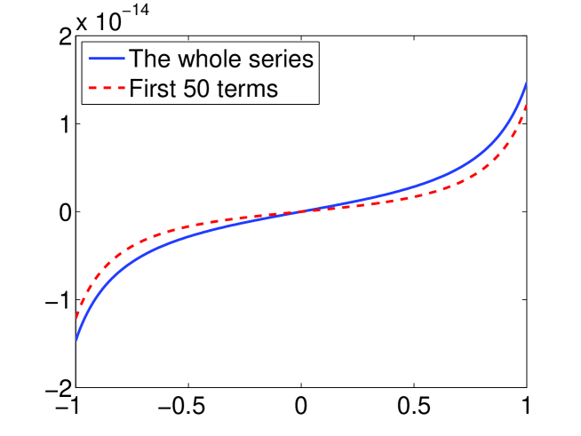
Figure 6: Illustration of Theorem 58 with $c=100$, $n=81$. $|\lambda_{n}|=\mbox{\text{\rm{0.19431E-07}}}$.

We are now ready to prove the principal theorem of this section. It is illustrated in Table 9 and in Figures 5, 6 (see Experiment 8 in Section 6.1.3).

Theorem 56.

Suppose that $c>1$, and that $n>0$ is an even positive integer. Suppose also that

$$n>\frac{2c}{\pi}+1,$$ (414)

that

$$|\lambda_{n}|<\frac{1}{10},$$ (415)

and that

$$\chi_{n}-c^{2}<\frac{c^{2}}{|\lambda_{n}|}.$$ (416)

Suppose furthermore that $-1<t_{1}<\dots<t_{n}<1$ are the roots of $\psi_{n}$ in $(-1,1)$, and that the function $I:(-1,1)\to\mathbb{R}$ is defined via the formula

$$I(t)=\frac{1}{\psi_{n}(t)}-\sum_{j=1}^{n}\frac{1}{\psi_{n}^{\prime}(t_{j})\cdot(t-t_{j})},$$ (417)

for $-1<t<1$. Then,

$$|I(t)|\leq|\lambda_{n}|\cdot I_{\max},$$ (418)

where the real number $I_{max}$ is defined via the formula

$$I_{\max}=24\cdot\log\left(\frac{2}{|\lambda_{n}|}\right)+13\cdot(\chi_{n})^{1/4}+40\cdot c\cdot|\lambda_{n}|+2\sqrt{2}.$$ (419)

Proof.

Suppose that $1<x_{1}<x_{2}<\dots$ are the roots of $\psi_{n}$ in $(1,\infty)$, and that $k$ is an integer satisfying the inequality (396) in Theorem 54. Suppose also that the real number $R_{k}$ is defined via (397) in Theorem 54, the contour $\Gamma_{k}$ in the complex plane is defined via (410) in Theorem 55, and that $x_{M}$ is the maximal root of $\psi_{n}$ in $(1,\infty)$; in other words,

$$1<x_{1}<\dots<x_{M}<R_{k}<x_{M+1}<\dots.$$ (420)

(We observe that $\psi_{n}(R_{k})\neq 0$ due to (398) in Theorem 54.) We combine (417), (420) and Theorem 27 of Section 2.8 to conclude that, for any real $-1<t<1$,

$$I(t)= \;\sum_{k=1}^{M}\left(\frac{1}{\psi_{n}^{\prime}(x_{k})\cdot(t-x_{k})}+\frac{1}{\psi_{n}^{\prime}(-x_{k})\cdot(t+x_{k})}\right)+$$

$$\;\frac{1}{2\pi i}\oint_{\Gamma_{k}}\frac{dz}{\psi_{n}(z)\cdot(z-t)}.$$ (421)

We combine the assumption that $c>1$ with Theorem 9 in Section 2.1 to conclude that

$$\sqrt{1+\frac{\sqrt{\chi_{n}}}{\pi}}<(\chi_{n})^{1/4}\cdot\sqrt{\frac{1}{\sqrt{2}}+\frac{1}{\pi}}.$$ (422)

We obtain the inequality (418) by taking the limit $k\to\infty$ and using (421), (422), Theorem 53 and Theorem 55. ∎

Remark 10.

The conclusion of Theorem 56 holds for odd values of $n$ as well. The proof is essentially the same, and is based on Theorems 48, 53, and obvious modifications of Theorems 54, 55.

Remark 11.

Suppose that the function $I:(-1,1)\to\mathbb{R}$ is defined via (417). If $n$ is even, then $I$ is an even function. If $n$ is odd, then $I$ is an odd function.

In the following theorem, we provide a simple condition on $n$ that implies the inequality $|\lambda_{n}|<0.1$.

Theorem 57.

Suppose that $c>30$, and that $n>0$ is an integer. Suppose also that

$$n>\frac{2c}{\pi}+5.$$ (423)

Then,

$$|\lambda_{n}|<\frac{1}{10}.$$ (424)

Proof.

Suppose first that

$$c>200\cdot\pi.$$ (425)

We combine (425) with (42), (43) in Section 2.1 to conclude that, in this case,

$$|\lambda_{n}|=\sqrt{\frac{2\pi\cdot\mu_{n}}{c}}<\sqrt{\frac{2\pi}{c}}<\frac{1}{10}.$$ (426)

On the other hand, suppose that

$$30\leq c\leq 200\cdot\pi.$$ (427)

We observe that the interval $\left[30,200\cdot\pi\right]$ is compact, and use this observation to verify numerically that, if (427) holds,

$$|\lambda_{\text{floor}(2c/\pi+5)}|<\frac{1}{50},$$ (428)

where, for a real number $a$, $\text{floor}(a)$ is the largest integer less than or equal to $a$. We combine Theorem 1 in Section 2.1, (428) and (426) to establish (424). ∎

In the following theorem, we summarize Theorems 46, 56, 57 and Remark 10.

Theorem 58.

Suppose that $c>0$ is a real number and $n>0$ is an integer. Suppose also that

$$c>30,$$ (429)

and that

$$n>\frac{2c}{\pi}+5.$$ (430)

Suppose furthermore that the function $I:(-1,1)\to\mathbb{R}$ is defined via the formula (417) in Theorem 56. Then,

$$|I(t)|\leq|\lambda_{n}|\cdot I_{\max},$$ (431)

where the real number $I_{max}$ is defined via the formula (419) in Theorem 56.

Proof.

We combine (429), (430) with Theorem 57 to conclude that the inequality (415) holds. Also, we combine (429), (415) with Theorem 46 to conclude that the inequality (416) holds. We combine these observations with Theorem 56 and Remark 10 to obtain (431). ∎

4.4 PSWF-based Quadrature and its Properties

In this subsection, we define PSWF-based quadratures of order $n$, find an upper bound on their error, and show that a prescribed absolute accuracy can be achieved by a proper choice of $n$.

The principal result of this section is Theorem 65.

Definition 2.

Suppose that $n>0$ is a positive integer, and that

$$-1<t_{1}<t_{2}<\dots<t_{n}<1$$ (432)

are the roots of $\psi_{n}$ the interval in $\left(-1,1\right)$. For each integer $j=1,\dots,n$, we define the function $\varphi_{j}:(-1,1)\to\mathbb{R}$ via the formula

$$\varphi_{j}(t)=\frac{\psi_{n}(t)}{\psi_{n}^{\prime}(t_{j})\left(t-t_{j}\right)}.$$ (433)

In addition, for each integer $j=1,\dots,n$, we define the real number $W_{j}$ via the formula

$$W_{j}=\int_{-1}^{1}\varphi_{j}(s)\;ds=\frac{1}{\psi_{n}^{\prime}(t_{j})}\int_{-1}^{1}\frac{\psi_{n}(s)\;ds}{s-t_{j}}.$$ (434)

We refer to the expression of the form

$$\sum_{j=1}^{n}W_{j}\cdot f(t_{j})$$ (435)

as the PSWF-based quadrature rule of order $n$. The points $t_{1},\dots,t_{n}$ and the numbers $W_{1},\dots,W_{n}$ are referred to as the nodes and the weights of the quadrature, respectively. The purpose of (435) is to approximate the integral of a bandlimited function $f$ over the interval $\left[-1,1\right]$.

4.4.1 Expansion of $\varphi_{j}$ into a Prolate Series

Suppose that $n>0$ is a positive integer. For every integer $j=1,\dots,n$, we define the function $\varphi_{j}:(-1,1)\to\mathbb{R}$ via (433). In the following theorem, we evaluate the inner product $\left<\varphi_{j},\psi_{m}\right>$ for arbitrary $m\neq n$. This theorem is illustrated in Tables 11, 12, Figure 7 (see Experiment 9 in Section 6.1.4).

Theorem 59.

Suppose that $n>0$ is a positive integer, and that $m\neq n$ is a non-negative integer. Suppose also that $1\leq j\leq n$ is an integer. Then,

$$\int_{-1}^{1}\frac{\psi_{n}(t)}{t-t_{j}}\;\psi_{m}(t)\;dt=\frac{\left|\lambda_{m}\right|^{2}\psi_{m}(t_{j})}{\left|\lambda_{m}\right|^{2}-\left|\lambda_{n}\right|^{2}}\cdot\Big{[}\int_{-1}^{1}\frac{\psi_{n}(t)\;dt}{t-t_{j}}+ic\lambda_{n}\Psi_{n}(1,t_{j})\Big{]},$$ (436)

where $t_{j}$ is given via (432) in Definition 2, and the complex-valued function $\Psi_{n}:(-1,1)^{2}\to\mathbb{C}$ is defined via the formula

$$\Psi_{n}(y,t)=\int_{0}^{y}\psi_{n}(x)e^{-icxt}dx.$$ (437)

Proof.

We combine (37) with (437) to obtain, for all real $-1<y<1$,

$$\int_{t=-1}^{1}\psi_{n}(t)\int_{x=0}^{y}\frac{d}{dx}\left[\frac{e^{icx(t-t_{j})}}{ic(t-t_{j})}\right]dx\;dt=\int_{x=0}^{y}e^{-icxt_{j}}\int_{t=-1}^{1}\psi_{n}(t)e^{icxt}dt\;dx=$$

$$\lambda_{n}\cdot\int_{0}^{y}\psi_{n}(x)e^{-icxt_{j}}dx=\lambda_{n}\cdot\Psi_{n}(y,t_{j}).$$ (438)

On the other hand,

$$\int_{t=-1}^{1}\psi_{n}(t)\int_{x=0}^{y}\frac{d}{dx}\left[\frac{e^{icx(t-t_{j})}}{ic(t-t_{j})}\right]dx\;dt=\frac{1}{ic}\int_{-1}^{1}\frac{\psi_{n}(t)}{t-t_{j}}\left(e^{icy(t-t_{j})}-1\right)dt=$$

$$\frac{e^{-icyt_{j}}}{ic}\int_{-1}^{1}\frac{\psi_{n}(t)}{t-t_{j}}e^{icyt}dt-\frac{1}{ic}\int_{-1}^{1}\frac{\psi_{n}(t)\;dt}{t-t_{j}}.$$ (439)

We combine (438) and (439) to obtain, for all real $-1<x<1$,

$$ic\lambda_{n}e^{icxt_{j}}\Psi_{n}(x,t_{j})+e^{icxt_{j}}\int_{-1}^{1}\frac{\psi_{n}(t)\;dt}{t-t_{j}}=\int_{-1}^{1}\frac{\psi_{n}(t)}{t-t_{j}}e^{icxt}dt.$$ (440)

We combine (37), (437) and (440) to obtain

$$\int_{-1}^{1}\frac{\psi_{n}(t)}{t-t_{j}}\;\psi_{m}(t)\;dt=\frac{1}{\lambda_{m}}\int_{x=-1}^{1}\psi_{m}(x)\int_{t=-1}^{1}\frac{\psi_{n}(t)}{t-t_{j}}e^{icxt}dt\;dx=$$

$$\frac{ic\lambda_{n}}{\lambda_{m}}\int_{-1}^{1}\psi_{m}(x)e^{icxt_{j}}\Psi_{n}(x,t_{j})\;dx+\frac{1}{\lambda_{m}}\left(\int_{-1}^{1}\psi_{m}(x)e^{icxt_{j}}dx\right)\left(\int_{-1}^{1}\frac{\psi_{n}(t)\;dt}{t-t_{j}}\right)$$

$$\frac{ic\lambda_{n}}{\lambda_{m}}\int_{-1}^{1}\frac{\partial\Psi_{m}}{\partial x}(x,-t_{j})\Psi_{n}(x,t_{j})\;dx+\psi_{m}(t_{j})\int_{-1}^{1}\frac{\psi_{n}(t)\;dt}{t-t_{j}}.$$ (441)

We observe that $\psi_{n}(-t_{j})=0$, and combine this observation with (37) in Section 2.1 and (437) to obtain

$$0=\frac{\psi_{n}(-t_{j})}{\lambda_{n}}=\int_{-1}^{1}\psi_{n}(t)e^{-ictt_{j}}\;dt=\Psi_{n}(1,t_{j})-\Psi_{n}(-1,t_{j}),$$ (442)

and also

$$\lambda_{m}\psi_{m}(t_{j})=\int_{-1}^{1}\psi_{m}(t)e^{ictt_{j}}dt=\Psi_{m}(1,-t_{j})-\Psi_{m}(-1,-t_{j}).$$ (443)

We combine (442), (443) to obtain

$$\left[\Psi_{m}(x,-t_{j})\Psi_{n}(x,t_{j})\right]_{x=-1}^{1} \;=\Psi_{n}(1,t_{j})\left(\Psi_{m}(1,-t_{j})-\Psi_{m}(-1,-t_{j})\right)$$

$$\;=\lambda_{m}\psi_{m}(t_{j})\Psi_{n}(1,t_{j}).$$ (444)

Also, we combine (37), Theorem 1 in Section 2.1 and (437) to obtain

$$\int_{-1}^{1}\Psi_{m}(x,-t_{j})\frac{\partial\Psi_{n}}{\partial x}(x,t_{j})\;dx=$$

$$\frac{1}{\lambda_{m}}\int_{x=-1}^{1}\psi_{n}(x)e^{-icxt_{j}}\int_{y=0}^{x}e^{icyt_{j}}\int_{t=-1}^{1}\psi_{m}(t)e^{icty}dt\;dy\;dx=$$

$$\frac{1}{\lambda_{m}}\int_{t=-1}^{1}\psi_{m}(t)\int_{x=-1}^{1}\psi_{n}(x)e^{-icxt_{j}}\int_{y=0}^{x}e^{ic(t_{j}+t)y}dy\;dx\;dt=$$

$$\frac{1}{\lambda_{m}}\int_{t=-1}^{1}\psi_{m}(t)\int_{x=-1}^{1}\psi_{n}(x)\left(\frac{e^{icxt}-e^{-icxt_{j}}}{ic(t_{j}+t)}\right)dx\;dt=$$

$$\frac{\lambda_{n}}{\lambda_{m}}\int_{-1}^{1}\frac{\psi_{m}(t)\psi_{n}(t)dt}{ic(t+t_{j})}=\frac{\left(-1\right)^{n+m+1}\lambda_{n}}{ic\lambda_{m}}\int_{-1}^{1}\frac{\psi_{n}(t)}{t-t_{j}}\;\psi_{m}(t)\;dt.$$ (445)

We combine Theorem 1 in Section 2.1 with (444), (445) to obtain

$$\frac{ic\lambda_{n}}{\lambda_{m}}\int_{-1}^{1}\frac{\partial\Psi_{m}}{\partial x}(x,-t_{j})\Psi_{n}(x,t_{j})\;dx=$$

$$\frac{ic\lambda_{n}}{\lambda_{m}}\cdot\left[\lambda_{m}\psi_{m}(t_{j})\Psi_{n}(1,t_{j})+\frac{\left(-1\right)^{n+m}\lambda_{n}}{ic\lambda_{m}}\int_{-1}^{1}\frac{\psi_{n}(t)}{t-t_{j}}\;\psi_{m}(t)\;dt\right]=$$

$$ic\lambda_{n}\psi_{m}(t_{j})\Psi_{n}(1,t_{j})+\frac{|\lambda_{n}|^{2}}{|\lambda_{m}|^{2}}\int_{-1}^{1}\frac{\psi_{n}(t)}{t-t_{j}}\;\psi_{m}(t)\;dt.$$ (446)

Finally, we recall that $m\neq n$ and substitute (446) into (441) to obtain (436). ∎

4.4.2 Quadrature Error

For a positive integer $n>0$, we define the PSWF-based quadrature of order $n$ via (432), (434) in Definition 2. This quadrature is used to approximate the integral of an arbitrary bandlimited function $f:(-1,1)\to\mathbb{C}$ over the interval $(-1,1)$ (see (4) in Section 1.1 and (435)). We refer to the difference

$$\int_{-1}^{1}f(t)\;dt-\sum_{j=1}^{n}f\left(t_{j}\right)\cdot W_{j}$$ (447)

as the “quadrature error” (for integrating $f$). The following theorem, illustrated in Tables 15, 16, provides an upper bound on the absolute value of the quadrature error (for integrating $\psi_{m}$ for arbitrary $m<n$). One of the principal goals of this paper is to investigate this error (see see (6) in Section 1.1). The results of additional numerical experiments, in which this quadrature is used for integration of certain functions, are summarized in Tables 16, 18 and Figures 9, 10, 11 (see Experiments 11, 12 in Section 6.2.1).

Theorem 60.

Suppose that $n>0$ and $0\leq m\leq n-1$ are integers. Suppose also that $t_{1},\dots,t_{n}$ and $W_{1},\dots,W_{n}$ are, respectively, the nodes and weights of the quadrature, introduced in Definition 2 above. Suppose furthermore that the real number $P_{n,m}$ is defined via the formula

$$P_{n,m}=\sum_{j=1}^{n}\frac{\psi_{m}(t_{j})}{\psi_{n}^{\prime}(t_{j})}\cdot\Psi_{n}(1,t_{j}),$$ (448)

where the complex-valued function $\Psi_{n}:(-1,1)^{2}\to\mathbb{C}$ is that of Theorem 59 above. Then,

$$\left|\int_{-1}^{1}\psi_{m}(s)\;ds-\sum_{j=1}^{n}\psi_{m}(t_{j})W_{j}\right|\leq$$

$$\left(1-\frac{\left|\lambda_{n}\right|^{2}}{\left|\lambda_{m}\right|^{2}}\right)\cdot\|I\|_{\infty}+\left|\lambda_{n}\right|\cdot\left(\frac{\left|\lambda_{n}\right|}{\left|\lambda_{m}\right|}\left|\psi_{m}(0)\right|+c\left|P_{n,m}\right|\right),$$ (449)

where $\|I\|_{\infty}$ is the $L^{\infty}$-norm of the function $I:(-1,1)\to\mathbb{R}$, defined via (417) in Theorem 56 in Section 4.3.3, i.e.

$$\|I\|_{\infty}=\sup\left\{|I(t)|\;:\;-1<t<1\right\}.$$ (450)

Proof.

Suppose that the function $I:(-1,1)\to\mathbb{R}$ is defined via (417) in Theorem 56 in Section 4.3.3. We multiply (417) by $\psi_{n}(t)\cdot\psi_{m}(t)$ to obtain, for all real $-1<t<1$,

$$\psi_{m}(t)=\sum_{j=1}^{n}\psi_{m}(t)\varphi_{j}(t)+\psi_{m}(t)\psi_{n}(t)I(t),$$ (451)

where, for each $j=1,\dots,n$, the function $\varphi_{j}:(-1,1)\to\mathbb{R}$ is that of Definition 2. We combine (37), Theorem 56, Definition 2, Theorem 59, (450), and integrate (451) over the interval $(-1,1)$ to obtain

$$\lambda_{m}\psi_{m}(0)=$$

$$\frac{\left|\lambda_{m}\right|^{2}}{\left|\lambda_{m}\right|^{2}-\left|\lambda_{n}\right|^{2}}\sum_{j=1}^{n}\psi_{m}(t_{j})\left(W_{j}+ic\lambda_{n}\frac{\Psi_{n}(1,t_{j})}{\psi_{n}^{\prime}(t_{j})}\right)+\xi\cdot\|I\|_{\infty},$$ (452)

where $-1\leq\xi\leq 1$ is a real number. We combine (452) with (448) to obtain

$$\left(1-\frac{|\lambda_{n}|^{2}}{|\lambda_{m}|^{2}}\right)\cdot\lambda_{m}\psi_{m}(0)=$$

$$\sum_{j=1}^{n}\psi_{m}(t_{j})W_{j}+ic\lambda_{n}P_{n,m}+\left(1-\frac{|\lambda_{n}|^{2}}{|\lambda_{m}|^{2}}\right)\cdot\xi\cdot\|I\|_{\infty}.$$ (453)

Finally, we rearrange (453) to obtain (449). ∎

In the following theorem, we establish an upper bound on $P_{n,m}$, defined via (448) above. This theorem is illustrated in Table 14 and Figure 8 (see Experiment 10 in Section 6.1.4).

Theorem 61.

Suppose that $n,m$ are non-negative integers, and that $0\leq m<n$. Suppose also that $\chi_{n}>c^{2}$, and that the real number $P_{n,m}$ is defined via (448) in Theorem 60. Then,

$$c\left|P_{n,m}\right|\leq\sqrt{32}\cdot n^{2}.$$ (454)

Proof.

Since $\chi_{n}>c^{2}$, the inequality

$$\psi_{n}^{2}(t)\leq\psi_{n}^{2}(1)\leq n+\frac{1}{2},$$ (455)

holds for all real $-1\leq t\leq 1$, due to Theorems 12, 13 in Section 2.1. Therefore,

$$\int_{1-1/8n}^{1}\psi_{n}^{2}(t)\;dt\leq\frac{1}{8}+\frac{1}{16n}<\frac{3}{16}.$$ (456)

We combine (456) with Theorem 1 in Section 2.1 to obtain

$$\int_{0}^{1-1/8n}\psi_{n}^{2}(t)\;dt=\int_{0}^{1}\psi_{n}^{2}(t)\;dt-\int_{1-1/8n}^{1}\psi_{n}^{2}(t)\;dt\geq\frac{1}{2}-\frac{3}{16}=\frac{5}{16}.$$ (457)

We observe that

$$\int\frac{dx}{\left(1-x^{2}\right)^{2}}=\frac{1}{2}\cdot\frac{x}{1-x^{2}}+\frac{1}{4}\log\frac{x+1}{1-x},$$ (458)

and combine (457) and (458) to obtain

$$\int_{0}^{1-1/8n}\frac{dx}{\left(1-x^{2}\right)^{2}}=\frac{1}{2}\cdot\frac{1-1/8n}{1-\left(1-1/8n\right)^{2}}+\frac{1}{4}\log\frac{2-1/8n}{1/8n}=$$

$$\frac{1}{2}\cdot\frac{8n\left(8n-1\right)}{16n-1}+\frac{1}{4}\log\left(16n-1\right)\leq 4n+n\leq 5n.$$ (459)

Suppose that the functions $Q(t),\tilde{Q}(t):(-1,1)\to\mathbb{R}$ are defined, respectively, via the formulae (76), (77) in Theorem 17 in Section 2.1. We apply Theorem 17 with $t_{0}=0$ and $0<t\leq 1$ to obtain

$$Q(0)\cdot\chi_{n} \;=Q(0)\cdot p(0)\cdot q(0)=\tilde{Q}(0)$$

$$\;\geq\tilde{Q}(t)=c^{2}\left[\psi_{n}^{2}(t)+\frac{\left(t^{2}-1\right)\left(\psi_{n}^{\prime}(t)\right)^{2}}{\left(c^{2}\cdot t^{2}-\chi_{n}\right)}\right]\cdot\left(1-t^{2}\right)\left(\chi_{n}/c^{2}-t^{2}\right)$$

$$\;\geq c^{2}\psi_{n}^{2}(t)\left(1-t^{2}\right)\left(\chi_{n}/c^{2}-t^{2}\right)\geq c^{2}\psi_{n}^{2}(t)\left(1-t^{2}\right)^{2}.$$ (460)

It follows from (457), (459) and (460) that

$$5n\cdot Q(0)\cdot\frac{\chi_{n}}{c^{2}}\geq Q(0)\cdot\frac{\chi_{n}}{c^{2}}\int_{0}^{1-1/8n}\frac{dx}{\left(1-x^{2}\right)^{2}}\geq\int_{0}^{1-1/8n}\psi_{n}^{2}(t)\;dt\geq\frac{5}{16},$$ (461)

which, in turn, implies that

$$\frac{1}{Q(0)}\leq 16n\cdot\frac{\chi_{n}}{c^{2}}.$$ (462)

Suppose now that $j\geq n/2$ is an integer, and $t_{j}$ is that of Definition 2. We combine (462) with Theorem 17 in Section 2.1 to obtain

$$\frac{\left(\psi_{n}^{\prime}(t_{j})\right)^{2}}{\chi_{n}}\geq\frac{(1-t_{j}^{2})\cdot\left(\psi_{n}^{\prime}(t_{j})\right)^{2}}{\chi_{n}-c^{2}t_{j}^{2}}=Q(t_{j})\geq Q(0)\geq\frac{c^{2}}{16n\cdot\chi_{n}}.$$ (463)

Due to Theorem 14 in Section 2.1, for all integer $0\leq m<n$ and real $-1<t<1$,

$$|\psi_{m}(t)|\leq 2\sqrt{n}.$$ (464)

We combine Theorem 1 in Section 2.1 with (437) of Theorem 59 above to obtain, for all real $0\leq t\leq 1$,

$$|\Psi_{n}(1,t)|=\left|\int_{0}^{1}\psi_{n}(x)e^{-icxt}\;dt\right|\leq\frac{1}{2}\int_{-1}^{1}|\psi_{n}(x)|\;dx\leq\frac{\sqrt{2}}{2}.$$ (465)

Finally, we combine (448), (463), (464) and (465) to obtain

$$c|P_{n,m}|\leq cn\cdot\max_{t_{j}\geq 0}\left|\frac{\psi_{m}(t_{j})}{\psi_{n}^{\prime}(t_{j})}\cdot\Psi_{n}(1,t_{j})\right|\leq cn\cdot\frac{\sqrt{16n}}{c}\cdot\frac{\sqrt{2}}{2}\cdot 2\sqrt{n},$$ (466)

which implies (454). ∎

Corollary 4.

Suppose that $m$ is an odd integer. Then, $P_{n,m}=0$.

Proof.

Suppose that $1\leq j\leq n$ is an integer, and $t_{1},\dots,t_{n}$ are the roots of $\psi_{n}$ in $(-1,1)$. We combine Theorem 1 and (37) in Section 2.1 with (437) to obtain, for every $j=1,\dots,n$,

$$(-1)^{n}\cdot\Psi_{n,j}(1)+\Psi_{n,n+1-j}(1)=$$

$$\int_{0}^{1}\psi_{n}(-x)e^{-icxt_{j}}\;dx+\int_{0}^{1}\psi_{n}(x)e^{icxt_{j}}\;dx=$$

$$\int_{-1}^{1}\psi_{n}(x)e^{icxt_{j}}\;dx=\lambda_{n}\psi_{n}(t_{j})=0.$$ (467)

We observe that $\psi_{n}^{\prime}$ is odd for even $n$ and even for odd $n$, and combine this observation with (467) to obtain, for every integer $j=1,\dots,n$,

$$\frac{\Psi_{n,j}(1)}{\psi_{n}^{\prime}(t_{j})}=\frac{\Psi_{n,n+1-j}(1)}{\psi_{n}^{\prime}(t_{n+1-j})}.$$ (468)

We combine (468) with (448) to obtain

$$P_{n,m} \;=\sum_{j=1}^{n}\psi_{m}(t_{j})\cdot\frac{\Psi_{n,j}(1)}{\psi_{n}^{\prime}(t_{j})}$$

$$\;=\sum_{j\leq n/2}\left(\psi_{m}(t_{j})+\psi_{m}(-t_{j})\right)\cdot\frac{\Psi_{n,j}(1)}{\psi_{n}^{\prime}(t_{j})}=0.$$ (469)

∎

In the following theorem, we simplify the inequality (449) of Theorem 60. It is illustrated in Table 18 and in Figure 9 (see Experiment 12 in Section 6.2.1). See also Conjecture 2 and Remark 26 in Section 6.2.1.

Theorem 62.

Suppose that $n>0$ and $0\leq m\leq n-1$ are integers. Suppose also that $t_{1},\dots,t_{n}$ and $W_{1},\dots,W_{n}$ are, respectively, the nodes and weights of the quadrature, introduced in Definition 2 above. Suppose furthermore that

$$c>30,$$ (470)

and that

$$n>\frac{2c}{\pi}+5.$$ (471)

Then,

$$\left|\int_{-1}^{1}\psi_{m}(s)\;ds-\sum_{j=1}^{n}\psi_{m}(t_{j})W_{j}\right|\leq|\lambda_{n}|\cdot\left(24\cdot\log\left(\frac{1}{|\lambda_{n}|}\right)+6\cdot\chi_{n}\right).$$ (472)

Proof.

We combine Theorems 1, 9, 14 in Section 2.1, the inequality (471) and Theorems 60, 61 to conclude that

$$\left|\int_{-1}^{1}\psi_{m}(s)\;ds-\sum_{j=1}^{n}\psi_{m}(t_{j})W_{j}\right|\leq\|I\|_{\infty}+|\lambda_{n}|\cdot(2\sqrt{n}+\sqrt{32}\cdot n^{2}),$$ (473)

where $\|I\|_{\infty}$ is defined via (450) in Theorem 60. Next, we combine (470), (471), Theorem 9 in Section 2.1, Theorems 57, 58 in Section 4.3.3 and (450) to conclude that

$$\|I\|_{\infty}\leq|\lambda_{n}|\cdot\left(24\cdot\log\left(\frac{2}{|\lambda_{n}|}\right)+13\cdot(\chi_{n})^{1/4}+4\sqrt{\chi_{n}}+2\sqrt{2}\right).$$ (474)

We combine (471) with Theorem 6 in Section 2.1 to conclude that

$$n<\sqrt{\chi_{n}}.$$ (475)

Also, we observe that, due to the combination of (470) and Theorem 9 in Section 2.1,

$$\sqrt{32}\cdot\chi_{n}+4\sqrt{\chi_{n}}+15\cdot(\chi_{n})^{1/4}+2\sqrt{2}+24\cdot\log(2)=$$

$$\chi_{n}\cdot\left(\sqrt{32}+4\cdot\chi_{n}^{-1/2}+15\cdot\chi_{n}^{-3/4}+(2\sqrt{2}+24\cdot\log(2))\cdot\chi_{n}^{-1}\right)<6\cdot\chi_{n}.$$ (476)

Now (472) follows from the combination of (473), (474), (475) and (476). ∎

The following theorem is a conclusion of Theorem 11 of Section 2.1 and Theorems 62, 57 above.

Theorem 63.

Suppose that $n>0$ and $0\leq m\leq n-1$ are integers. Suppose also that $t_{1},\dots,t_{n}$ and $W_{1},\dots,W_{n}$ are, respectively, the nodes and weights of the quadrature, introduced in Definition 2 above. Suppose furthermore that

$$c>30,$$ (477)

and that

$$n>\frac{2c}{\pi}+7.$$ (478)

Then,

$$\left|\int_{-1}^{1}\psi_{m}(s)\;ds-\sum_{j=1}^{n}\psi_{m}(t_{j})W_{j}\right|\leq 14340\cdot\frac{\chi_{n}^{5}}{c^{7}}\cdot\exp\left[-\frac{\pi}{4}\cdot\frac{\chi_{n}-c^{2}}{\sqrt{\chi_{n}}}\right].$$ (479)

Proof.

We combine (477), (478) with Theorem 62 above to obtain

$$\left|\int_{-1}^{1}\psi_{m}(s)\;ds-\sum_{j=1}^{n}\psi_{m}(t_{j})W_{j}\right|\leq|\lambda_{n}|\cdot\left(24\cdot\log\left(\frac{1}{|\lambda_{n}|}\right)+6\cdot\chi_{n}\right).$$ (480)

Suppose first that

$$|\lambda_{n}|\leq\exp\left[-\frac{\chi_{n}}{4}\right].$$ (481)

Then,

$$|\lambda_{n}|\cdot\left(24\cdot\log\left(\frac{1}{|\lambda_{n}|}\right)+6\cdot\chi_{n}\right)\leq 48\cdot|\lambda_{n}|\cdot\log\left(\frac{1}{|\lambda_{n}|}\right).$$ (482)

We combine (477), (481) and Theorem 4 in Section 2.1 to conclude that

$$|\lambda_{n}|<\exp\left[-\frac{c^{2}}{4}\right]<e^{-225}<e^{-1}.$$ (483)

We combine (481), (482) and (483) to obtain

$$|\lambda_{n}|\cdot\left(24\cdot\log\left(\frac{1}{|\lambda_{n}|}\right)+6\cdot\chi_{n}\right)\leq 48\cdot|\lambda_{n}|\cdot\log\left(\frac{1}{|\lambda_{n}|}\right)\leq$$

$$48\cdot\exp\left[-\frac{\chi_{n}}{4}\right]\cdot\frac{\chi_{n}}{4}=12\cdot\chi_{n}\cdot\exp\left[-\frac{\chi_{n}}{4}\right].$$ (484)

Suppose, on the other hand, that

$$\exp\left[-\frac{\chi_{n}}{4}\right]<|\lambda_{n}|<\frac{1}{10}$$ (485)

(note that the right-hand side inequality in (485) follows from the combination of (477), (478) and Theorem 57). It follows from (485) that, in this case,

$$|\lambda_{n}|\cdot\left(24\cdot\log\left(\frac{1}{|\lambda_{n}|}\right)+6\cdot\chi_{n}\right)\leq 12\cdot\chi_{n}\cdot|\lambda_{n}|.$$ (486)

We combine (478) with Theorem 11 to obtain

$$|\lambda_{n}|<1195\cdot\frac{\chi_{n}^{4}}{c^{7}}\cdot\exp\left[-\frac{\pi}{4}\cdot\frac{\chi_{n}-c^{2}}{\sqrt{\chi_{n}}}\right].$$ (487)

We combine (477) with Theorem 4 of Section 2.1 to conclude that

$$\exp\left[-\frac{\chi_{n}}{4}\right]<1195\cdot\frac{\chi_{n}^{4}}{c^{7}}\cdot\exp\left[-\frac{\pi}{4}\cdot\frac{\chi_{n}-c^{2}}{\sqrt{\chi_{n}}}\right].$$ (488)

We combine (481), (484), (485), (486), (487), (488) that

$$|\lambda_{n}|\cdot\left(24\cdot\log\left(\frac{1}{|\lambda_{n}|}\right)+6\cdot\chi_{n}\right)\leq$$

$$12\cdot\chi_{n}\cdot 1195\cdot\frac{\chi_{n}^{4}}{c^{7}}\cdot\exp\left[-\frac{\pi}{4}\cdot\frac{\chi_{n}-c^{2}}{\sqrt{\chi_{n}}}\right].$$ (489)

Now (479) follows from the combination of (480) and (489). ∎

4.4.3 The Principal Result

In Theorem 63, we established an upper bound on the quadrature error for integrating $\psi_{m}$ (see (479)). However, this bound depends on $\chi_{n}$. In particular, it is not obvious how large $n$ should be to make sure that the quadrature error does not exceed given $\varepsilon>0$. In this subsection, we eliminate this inconvenience.

The following theorem is illustrated in Table 19 (see Experiment 14 in Section 6.2.1).

Theorem 64.

Suppose that $c>0$ is a positive real number, and that

$$c>30.$$ (490)

Suppose also that $\varepsilon>0$ is a positive real number, and that

$$0<\log\frac{1}{\varepsilon}<\frac{5\cdot\pi}{4\sqrt{6}}\cdot c-3\cdot\log(c)-\log(6^{5}\cdot 14340).$$ (491)

Suppose furthermore that the real number $\alpha$ is defined via the formula

$$\alpha=\frac{4\sqrt{6}}{\pi}\cdot\left(\log\frac{1}{\varepsilon}+3\cdot\log(c)+\log(6^{5}\cdot 14340)\right),$$ (492)

and that the real number $\nu(\alpha)$ is defined via the formula

$$\nu(\alpha)=\frac{2c}{\pi}+\frac{\alpha}{2\pi}\cdot\log\left(\frac{16ec}{\alpha}\right).$$ (493)

Suppose, in addition, that $n>0$ and $0\leq m\leq n-1$ are integers, and that

$$n>\nu(\alpha).$$ (494)

Then,

$$\left|\int_{-1}^{1}\psi_{m}(s)\;ds-\sum_{j=1}^{n}\psi_{m}(t_{j})W_{j}\right|<\varepsilon,$$ (495)

where $t_{j}$, $W_{j}$ are defined, respectively, via (432), (434) in Definition 2.

Proof.

It follows from (491) that

$$5c>\alpha>\frac{4\sqrt{6}}{\pi}\cdot\left(3\cdot\log(c)+\log(6^{5}\cdot 14340)\right),$$ (496)

where $\alpha$ is defined via (492). We observe that

$$\frac{d}{d\alpha}\left[\alpha\cdot\log\left(\frac{16ec}{\alpha}\right)\right]=\log\left(\frac{16c}{\alpha}\right),$$ (497)

and hence the function $\nu:(0,16c)\to\mathbb{R}$, defined via (493), is monotonically increasing. We combine (490), (492), (496), (497) to conclude that

$$\frac{2c}{\pi}+30<\nu(\alpha)<\frac{2c}{\pi}+\frac{5c}{2\pi}\cdot\log\left(\frac{16e}{5}\right)<\frac{5c}{2}.$$ (498)

We combine Theorem 7 of Section 2.1 with (493), (494) and (496) to obtain the inequality

$$\chi_{n}>c^{2}+\alpha\cdot c.$$ (499)

Suppose now that the function $f:(c,\infty)\to\mathbb{R}$ is defined via the formula

$$f(y)=y^{10}\cdot\exp\left[-\frac{\pi}{4}\cdot\frac{y^{2}-c^{2}}{y}\right].$$ (500)

We differentiate (500) with respect to $y$ and use (490) to obtain

$$f^{\prime}(y)=\frac{f(y)}{y}\cdot\left[10-y\cdot\frac{\pi}{4}\cdot\left(1+\frac{c^{2}}{y^{2}}\right)\right]<0,$$ (501)

for all $y>c$. We combine (490), (498), (499), (500), (501) with Theorem 63 to conclude that

$$\left|\int_{-1}^{1}\psi_{m}(s)\;ds-\sum_{j=1}^{n}\psi_{m}(t_{j})W_{j}\right|\leq$$

$$14340\cdot\frac{\chi_{n}^{5}}{c^{7}}\cdot\exp\left[-\frac{\pi}{4}\cdot\frac{\chi_{n}-c^{2}}{\sqrt{\chi_{n}}}\right]\leq$$

$$14340\cdot c^{3}\cdot\left(1+\frac{\alpha}{c}\right)^{5}\cdot\exp\left[-\frac{\pi}{4}\cdot\frac{\alpha}{\sqrt{1+\alpha/c}}\right].$$ (502)

We combine (496), (502) to obtain

$$\left|\int_{-1}^{1}\psi_{m}(s)\;ds-\sum_{j=1}^{n}\psi_{m}(t_{j})W_{j}\right|\leq 14340\cdot 6^{5}\cdot c^{3}\cdot\exp\left[-\frac{\pi}{4}\cdot\frac{\alpha}{\sqrt{6}}\right].$$ (503)

Now (495) follows from the combination of (492) and (503). ∎

The following theorem is a direct consequence of Theorem 64. This theorem is one of the principal results of the paper. It is illustrated in Table 19 (see Experiment 14 in Section 6.2.1). See also Conjecture 2 in Section 6.2.1.

Theorem 65.

Suppose that $c>0$ is a positive real number, and that

$$c>30.$$ (504)

Suppose also that $\varepsilon>0$ is a positive real number, and that

$$\exp\left[-\frac{3}{2}\cdot(c-20)\right]<\varepsilon<1.$$ (505)

Suppose furthermore that $n>0$ and $0\leq m<n$ are positive integers, and that

$$n>\frac{2c}{\pi}+\left(10+\frac{3}{2}\cdot\log(c)+\frac{1}{2}\cdot\log\frac{1}{\varepsilon}\right)\cdot\log\left(\frac{c}{2}\right).$$ (506)

Then,

$$\left|\int_{-1}^{1}\psi_{m}(s)\;ds-\sum_{j=1}^{n}\psi_{m}(t_{j})W_{j}\right|<\varepsilon,$$ (507)

where $t_{j}$, $W_{j}$ are defined, respectively, via (432), (434) in Definition 2.

Proof.

We observe that, for all real $x>30$,

$$\frac{3}{2}\cdot(x-20)<\frac{5\cdot\pi}{4\sqrt{6}}\cdot x-3\cdot\log(x)-\log(6^{5}\cdot 14340).$$ (508)

Also, we combine (504), (505) to conclude that

$$\frac{4\sqrt{6}}{2\pi^{2}}\cdot\left(\log\frac{1}{\varepsilon}+3\cdot\log(c)+\log(6^{5}\cdot 14340)\right)<10+\frac{3}{2}\cdot\log(c)+\frac{1}{2}\cdot\log\frac{1}{\varepsilon}.$$ (509)

Furthermore, we combine (504), (505) to conclude that

$$\frac{4\sqrt{6}}{\pi}\cdot\left(\log\frac{1}{\varepsilon}+3\cdot\log(c)+\log(6^{5}\cdot 14340)\right)>89>2\cdot 16e.$$ (510)

Now (507) follows from the combination of (504), (505), (506), (508), (509), (510) and Theorem 64. ∎

The assumptions of Theorem 65 contain a minor inconvenience - namely, the parameter $\varepsilon$ is not allowed to be “too small” (in the sense of (505)). In the following theorem, we eliminate this restriction. On the other hand, for the values of $\varepsilon$ in the range (505), the resulting inequality for $n$ is much weaker than (506).

Theorem 66.

Suppose that $c>0$ is a positive real number, and that

$$c>30.$$ (511)

Suppose also that $\varepsilon>0$ is a positive real number, and that

$$0<\varepsilon<1.$$ (512)

Suppose furthermore that $n>0$ and $0\leq m<n$ are positive integers, and that

$$n\cdot\left(1-\frac{40}{\pi c}\right)>c+\frac{12}{\pi}\cdot\log(c)+\frac{4}{\pi}\cdot\log\frac{1}{\varepsilon}.$$ (513)

Then,

$$\left|\int_{-1}^{1}\psi_{m}(s)\;ds-\sum_{j=1}^{n}\psi_{m}(t_{j})W_{j}\right|<\varepsilon,$$ (514)

where $t_{j}$, $W_{j}$ are defined, respectively, via (432), (434) in Definition 2.

Proof.

We combine (513) with Theorem 6 in Section 2.1 and (109) in Section 2.3 to conclude that

$$c^{2}<n^{2}<\chi_{n}.$$ (515)

Also, we combine (511), (512), (513), (515) with Theorem 63 and (501) in the proof of Theorem 64 to conclude that

$$\left|\int_{-1}^{1}\psi_{m}(s)\;ds-\sum_{j=1}^{n}\psi_{m}(t_{j})W_{j}\right|\leq$$

$$14340\cdot\frac{\chi_{n}^{5}}{c^{7}}\cdot\exp\left[-\frac{\pi}{4}\cdot\frac{\chi_{n}-c^{2}}{\sqrt{\chi_{n}}}\right]\leq$$

$$14340\cdot c^{3}\cdot\left(\frac{n}{c}\right)^{10}\cdot\exp\left[-\frac{\pi}{4}\cdot c\cdot\left(\frac{n}{c}-\frac{c}{n}\right)\right].$$ (516)

We take the logarithm of both sides of (516) and use (515) to obtain

$$\log\left|\int_{-1}^{1}\psi_{m}(s)\;ds-\sum_{j=1}^{n}\psi_{m}(t_{j})W_{j}\right|<$$

$$\log(14340)+3\cdot\log(c)+10\cdot\log\left(\frac{n}{c}\right)-\frac{\pi}{4}\cdot n+\frac{\pi}{4}\cdot c<$$

$$\log(14340)+3\cdot\log(c)+10\cdot\left(\frac{n}{c}\right)-10-\frac{\pi}{4}\cdot n+\frac{\pi}{4}\cdot c<$$

$$\frac{\pi}{4}\cdot\left(\frac{12}{\pi}\cdot\log(c)-n\cdot\left(1-\frac{40}{\pi c}\right)+c\right).$$ (517)

Now (514) follows from the combination of (513) and (517). ∎

4.4.4 Quadrature Weights

In this subsection, we analyze the weights $W_{1},\dots,W_{n}$ of the quadrature, defined in Definition 2 in Section 4.4. This analysis has two principal purposes. On the one hand, it provides the basis for a fast algorithm for the evaluation of the weights. On the other hand, it provides a theoretical explanation of some empirically observed properties of the weights.

The results of this subsection are illustrated in Table 20 and in Figure 12 (see Experiment 15 in Section 6.2.2).

In the following theorem, we describe a function, whose values at the roots $t_{1},\dots,t_{n}$ of $\psi_{n}$ in $(-1,1)$ are equal to the quadrature weights $W_{1},\dots,W_{n}$, up to a certain scaling.

Theorem 67.

Suppose that $n$ is a non-negative integer. Suppose also that the function $\tilde{\Phi}_{n}:(-1,1)\to\mathbb{R}$ is defined via the formula

$$\tilde{\Phi}_{n}(t)=\sum_{k=0}^{\infty}\alpha_{k}^{(n)}Q_{k}(t),$$ (518)

where $Q_{k}(t)$ is the $k$th Legendre function of the second kind, defined in Section 2.2, and $\alpha_{k}^{(n)}$ is the $k$th coefficient of the Legendre expansion of $\psi_{n}$, defined via (84) in Section 2.2. Suppose furthermore that $t_{1}<\dots<t_{n}$ are the roots of $\psi_{n}$ in $(-1,1)$. Then, for every integer $j=1,2,\dots,n$,

$$\tilde{\Phi}_{n}(t_{j})=\frac{1}{2}\int_{-1}^{1}\frac{\psi_{n}(t)\;dt}{t_{j}-t}.$$ (519)

Proof.

Suppose that $1\leq j\leq n$ is an integer, and that $\delta>0$ is a positive real number. We combine (518) with (82), (83), (84), (103) in Section 2.2 to obtain

$$\sum_{k=0}^{\infty}\alpha_{k}^{(n)}Q_{k}(t_{j}+i\delta)=\frac{1}{2}\int_{-1}^{1}\frac{\psi_{n}(t)\;dt}{t_{j}+i\delta-t},$$ (520)

provided that $\delta$ is sufficiently small. Suppose now that $\varepsilon>0$ is a real number, and that

$$\varepsilon<\frac{1}{2}\cdot\min\left\{|t_{j}-1|,\;|t_{j}+1|\right\}.$$ (521)

We observe that, since $t_{j}$ is a root of $\psi_{n}$, the right-hand side of (519) is well defined. We combine this observation with (520), (521) to evaluate

$$\lim_{\delta\to 0,\;\delta>0}\left(\frac{1}{2}\int_{t_{j}-\varepsilon}^{t_{j}+\varepsilon}\frac{\psi_{n}(t)\;dt}{t_{j}+i\delta-t}-\frac{1}{2}\int_{t_{j}-\varepsilon}^{t_{j}+\varepsilon}\frac{\psi_{n}(t)\;dt}{t_{j}-t}\right)=$$

$$\lim_{\delta\to 0,\;\delta>0}\frac{1}{2}\int_{-\varepsilon}^{\varepsilon}\psi_{n}(t_{j}+s)\cdot\left(\frac{1}{s+i\delta}-\frac{1}{s}\right)ds=$$

$$-\lim_{\delta\to 0,\;\delta>0}\frac{i\delta\cdot\psi_{n}^{\prime}(t_{j})}{2}\int_{-\varepsilon}^{\varepsilon}\frac{ds}{s+i\delta}=$$

$$\lim_{\delta\to 0,\;\delta>0}\delta\cdot\psi_{n}^{\prime}(t_{j})\cdot\arctan\left(\frac{\varepsilon}{\delta}\right)=0.$$ (522)

We combine (518), (520), (522) to obtain (519). ∎

The following corollary is a direct consequence of Definition 2 and Theorem 67.

Corollary 5.

Suppose that $n>0$ and $1\leq j\leq n$ are positive integers. Suppose also that the function $\tilde{\Phi}_{n}:(-1,1)\to\mathbb{R}$ is defined via (518) in Theorem 67. Then,

$$W_{j}=-2\cdot\frac{\tilde{\Phi}_{n}(t_{j})}{\psi_{n}^{\prime}(t_{j})},$$ (523)

where $t_{j}$, $W_{j}$ are defined, respectively, via (432), (434) of Definition 2.

Corollary 5 is illustrated in Table 20. We observe that Theorem 67 and Corollary 5 describe a connection between the weights $W_{1},\dots,W_{n}$ and the values of $\tilde{\Phi}_{n}$ at $t_{1},\dots,t_{n}$, where the function $\tilde{\Phi}_{n}$ is defined via (518). In the following theorem, we prove that $\tilde{\Phi}_{n}$ satisfies a certain second-order non-homogeneous ODE, closely related to the prolate ODE (48) in Section 2.1.

Theorem 68.

Suppose that $n$ is a non-negative integer, and that the function $\tilde{\Phi}_{n}:(-1,1)\to\mathbb{R}$ is defined via (518) in Theorem 67. Suppose also that the second-order differential operator $L_{n}$ is defined via the formula

$$L_{n}\left[\varphi\right](t)=\left(1-t^{2}\right)\varphi^{\prime\prime}(t)-2t\varphi^{\prime}(t)+\left(\chi_{n}-c^{2}t^{2}\right)\varphi(t).$$ (524)

Then, in the interval $(-1,1)$ the function $\tilde{\Phi}_{n}$ satisfies the nonhomogeneous ODE

$$L_{n}\left[\tilde{\Phi}_{n}\right](t)=-c^{2}\left(\alpha_{0}^{(n)}t+\alpha_{1}^{(n)}/3\right),$$ (525)

where the coefficients $\alpha_{0}^{(n)},\alpha_{1}^{(n)}$ are the first two coefficients of the Legendre expansion of $\psi_{n}$, defined via (84) in Section 2.2.

Proof.

We combine (102), (98) of Section 2.2 with (524) to obtain

$$L_{n}\left[Q_{k}\right]=\left(\chi_{n}-k(k+1)-c^{2}t^{2}\right)\cdot Q_{k},$$ (526)

where $Q_{k}$ is the $k$th Legendre function of the second kind, defined in Section 2.2. We combine (98) of Section 2.2 with (526) to obtain

$$L_{n}\left[\sum_{k=0}^{\infty}\alpha_{k}^{(n)}Q_{k}\right]=\sum_{k=0}^{\infty}\alpha_{k}^{(n)}\left(\chi_{n}-k(k+1)-c^{2}t^{2}\right)Q_{k}=$$

$$\sum_{k=0}^{\infty}\alpha_{k}^{(n)}\left(\chi_{n}-k(k+1)\right)Q_{k}$$

$$\;\quad-c^{2}\sum_{k=0}^{\infty}\alpha_{k}^{(n)}\left(A_{k-2}Q_{k-2}+B_{k}Q_{k}+C_{k+2}Q_{k+2}\right)=$$

$$\sum_{k=2}^{\infty}\left[\left(\chi_{n}-k(k+1)\right)\alpha_{k}^{(n)}-c^{2}\left(\alpha_{k+2}^{(n)}A_{k}+\alpha_{k}^{(n)}B_{k}+\alpha_{k-2}^{(n)}C_{k}\right)\right]Q_{k}$$

$$\;\quad+\left[\left(\chi_{n}-1(1+1)\right)\alpha_{1}^{(n)}-c^{2}\left(\alpha_{3}^{(n)}A_{1}+\alpha_{1}^{(n)}B_{1}\right)\right]Q_{1}$$

$$\;\quad+\left[\left(\chi_{n}-0(0+1)\right)\alpha^{(n)}_{0}-c^{2}\left(\alpha_{2}^{(n)}A_{0}+\alpha_{0}^{(n)}B_{0}\right)\right]Q_{0}$$

$$\;\quad-c^{2}\left(\alpha_{1}^{(n)}\left(t^{2}Q_{1}-B_{1}Q_{1}-C_{3}Q_{3}\right)+\alpha_{0}^{(n)}\left(t^{2}Q_{0}-B_{0}Q_{0}-C_{2}Q_{2}\right)\right),$$ (527)

where $A_{k},B_{k},C_{k}$ are defined, respectively, via (99), (100), (101) in Section 2.2. By the same token, (527) holds, if we replace $Q_{k}$’s with $P_{k}$’s, where $P_{k}$ is the $k$th Legendre polynomial defined in Section 2.2. In other words,

$$L_{n}\left[\sum_{k=0}^{\infty}\alpha_{k}^{(n)}P_{k}\right]=$$

$$\sum_{k=2}^{\infty}\left[\left(\chi_{n}-k(k+1)\right)\alpha_{k}^{(n)}-c^{2}\left(\alpha_{k+2}^{(n)}A_{k}+\alpha_{k}^{(n)}B_{k}+\alpha_{k-2}^{(n)}C_{k}\right)\right]P_{k}$$

$$\;\quad+\left[\left(\chi_{n}-1(1+1)\right)\alpha_{1}^{(n)}-c^{2}\left(\alpha_{3}^{(n)}A_{1}+\alpha_{1}^{(n)}B_{1}\right)\right]P_{1}$$

$$\;\quad+\left[\left(\chi_{n}-0(0+1)\right)\alpha^{(n)}_{0}-c^{2}\left(\alpha_{2}^{(n)}A_{0}+\alpha_{0}^{(n)}B_{0}\right)\right]P_{0}$$

$$\;\quad-c^{2}\left(\alpha_{1}^{(n)}\left(t^{2}P_{1}-B_{1}P_{1}-C_{3}P_{3}\right)+\alpha_{0}^{(n)}\left(t^{2}P_{0}-B_{0}P_{0}-C_{2}P_{2}\right)\right),$$ (528)

We combine (78), (98) of Section 2.2 to conclude that

$$t^{2}\cdot P_{1}(t)-B_{1}\cdot P_{1}(t)-C_{3}\cdot P_{3}(t)=0,$$

$$t^{2}\cdot P_{0}(t)-B_{0}\cdot P_{0}(t)-C_{2}\cdot P_{2}(t)=0.$$ (529)

We recall that $\left\{P_{k}\right\}$ form an orthogonal system in $L^{2}\left[-1,1\right]$, and combine this observation with (48) in Section 2.1, (82) in Section 2.2, (524), (528) and (529) to conclude that, for every integer $k\geq 2$,

$$\left(\chi_{n}-k(k+1)\right)\alpha_{k}^{(n)}-c^{2}\left(\alpha_{k+2}^{(n)}A_{k}+\alpha_{k}^{(n)}B_{k}+\alpha_{k-2}^{(n)}C_{k}\right)=0,$$ (530)

and also

$$\left(\chi_{n}-1(1+1)\right)\alpha_{1}^{(n)}-c^{2}\left(\alpha_{3}^{(n)}A_{1}+\alpha_{1}^{(n)}B_{1}\right)=0,$$

$$\left(\chi_{n}-0(0+1)\right)\alpha^{(n)}_{0}-c^{2}\left(\alpha_{2}^{(n)}A_{0}+\alpha_{0}^{(n)}B_{0}\right)=0.$$ (531)

We substitute (530), (531) into (527) and use (518) to obtain

$$L_{n}\left[\tilde{\Phi}_{n}\right](t) \;=L_{n}\left[\sum_{k=0}^{\infty}\alpha_{k}^{(n)}Q_{k}\right](t)=$$

$$\;-c^{2}\alpha_{1}^{(n)}\left(t^{2}Q_{1}(t)-B_{1}Q_{1}(t)-C_{3}Q_{3}(t)\right)$$

$$\;-c^{2}\alpha_{0}^{(n)}\left(t^{2}Q_{0}(t)-B_{0}Q_{0}(t)-C_{2}Q_{2}(t)\right).$$ (532)

We combine (95), (97), (100), (101) of Section 2.2 to obtain

$$t^{2}Q_{0}(t)-B_{0}Q_{0}(t)-C_{2}Q_{2}(t)=$$

$$\left(t^{2}-\frac{1}{3}\right)\frac{1}{2}\log\frac{1+t}{1-t}-\frac{2}{3}\left(\frac{1}{4}\left(3t^{2}-1\right)\log\frac{1+t}{1-t}-\frac{3}{2}t\right)=t$$ (533)

and

$$t^{2}Q_{1}(t)-B_{1}Q_{1}(t)-C_{3}Q_{3}(t)=$$

$$\left(t^{2}-\frac{3}{5}\right)\left(\frac{t}{2}\log\frac{1+t}{1-t}-1\right)-\frac{2}{5}\left(\frac{1}{4}\left(5t^{3}-3t\right)\log\frac{1+t}{1-t}-\frac{5}{2}t^{2}+\frac{2}{3}\right)=$$

$$\left(\frac{t}{2}\left(t^{2}-\frac{3}{5}\right)-\frac{1}{10}\left(5t^{2}-3t\right)\right)\log\frac{1+t}{1-t}-t^{2}+\frac{3}{5}+t^{2}-\frac{4}{15}=\frac{1}{3}.$$ (534)

Finally, we substitute (533), (534) into (532) to obtain (525). ∎

In the following corollary, we establish a recurrence relation between the derivatives of $\tilde{\Phi}_{n}$ of arbitrary order (compare to Theorem 15 in Section 2.1).

Corollary 6.

Suppose that the function $\tilde{\Phi}_{n}:(-1,1)\to\mathbb{R}$ is defined via (518) of Theorem 67. Suppose also that $-1<t<1$ is a real number. Then,

$$\left(1-t^{2}\right)\cdot\tilde{\Phi}_{n}^{\prime\prime\prime}(t)-4t\cdot\tilde{\Phi}_{n}^{\prime\prime}(t)+\left(\chi_{n}-c^{2}t^{2}-2\right)\cdot\tilde{\Phi}_{n}^{\prime}(t)-2c^{2}t\cdot\tilde{\Phi}_{n}(t)=$$

$$-c^{2}\alpha_{0}^{(n)},$$ (535)

where $\alpha_{0}^{(n)}$ is defined via (84) in Section 2.2 (compare to (72) of Theorem 15 in Section 2.1). Also, for every integer $k\geq 2$,

$$\left(1-t^{2}\right)\tilde{\Phi}_{n}^{(k+2)}(t)-2\left(k+1\right)t\tilde{\Phi}_{n}^{(k+1)}(t)+\left(\chi_{n}-k\left(k+1\right)-c^{2}t^{2}\right)\tilde{\Phi}_{n}^{(k)}(t)$$

$$\quad\quad-c^{2}kt\tilde{\Phi}_{n}^{(k-1)}(t)-c^{2}k\left(k-1\right)\tilde{\Phi}_{n}^{(k-2)}(t)=0.$$ (536)

In other words, the higher order derivatives of $\tilde{\Phi}_{n}$ and $\psi_{n}$ satisfy the same recurrence relation (73) (see Theorem 15 in Section 2.1).

Proof.

To prove (535), we differentiate both sides of (525) with respect to $t$. To prove (536), we observe that the second derivative of the right-hand side of (525) is identically zero, and combine this observation with Theorem 15 in Section 2.1. ∎

The rest of this subsection is devoted to establishing the positivity of the quadrature weights $W_{1},\dots,W_{n}$, defined via (434) in Definition 2. The principal result of this part is Theorem 73 (see also Remarks 12, 13).

Theorem 69.

Suppose that $c>0$ is a real number, and that $n>0$ is an odd integer. Suppose also that $t_{1},t_{2},\dots,t_{n}$ and $W_{1},W_{2},\dots,W_{n}$ are defined, respectively, via (432), (434) in Definition 2. Suppose furthermore that the integer $j_{0}$ is defined via the formula

$$j_{0}=\frac{n+1}{2}.$$ (537)

Then, for every integer $j=1,\dots,n$,

$$\frac{\left(\psi_{n}^{\prime}(t_{j})\right)^{2}\cdot(1-t_{j}^{2})}{\left(\psi_{n}^{\prime}(0)\right)^{2}}\cdot W_{j}=W_{j_{0}}+\frac{ic\lambda_{n}}{\psi_{n}^{\prime}(0)}\int_{0}^{t_{j}}\psi_{n}(t)\;dt.$$ (538)

Proof.

Suppose that the differential operator $L_{n}$ is defined via (524) in Theorem 68. Suppose also that the function $\Phi_{n}:(-1,1)\to\mathbb{R}$ is the solution of the homogeneous second-order ODE

$$L_{n}\left[\varphi\right]=0$$ (539)

in the interval $(-1,1)$ with the initial conditions

$$\Phi_{n}(0)=\frac{1}{\psi_{n}^{\prime}(0)},\quad\Phi_{n}^{\prime}(0)=0.$$ (540)

Obviously, $\Phi_{n}$ is an even function. Moreover,

$$\Phi_{n}(t)\cdot\psi_{n}^{\prime}(t)-\Phi_{n}^{\prime}(t)\cdot\psi_{n}(t)=\frac{1}{1-t^{2}}$$ (541)

for all real $-1<t<1$ (this is the classical Abel’s formula; see e.g. Theorem 3.3.2 in [5]). Suppose that the function $\tilde{\Phi}_{n}:(-1,1)\to\mathbb{R}$ is defined via (518) in Theorem 67. We combine (525) of Theorem 68 with (598) to conclude that $\tilde{\Phi}_{n}$ satisfies the non-homogeneous ODE

$$L_{n}\left[\tilde{\Phi}_{n}\right](x)=\frac{ic\lambda_{n}\psi_{n}^{\prime}(0)}{2},$$ (542)

for all real $-1<x<1$. We observe that $\psi_{n},\Phi_{n}$ are two independent solutions of the ODE (539), and combine this observation with (542) to conclude that, for all real $-1<x<1$,

$$\tilde{\Phi}_{n}(x)= \;C_{1}\cdot\psi_{n}(x)+C_{2}\cdot\Phi_{n}(x)\;+$$

$$\;\frac{ic\lambda_{n}\psi_{n}^{\prime}(0)}{2}\cdot\left(\psi_{n}(x)\int_{0}^{x}\Phi_{n}(t)\;dt-\Phi_{n}(x)\int_{0}^{x}\psi_{n}(t)\;dt\right),$$ (543)

for some constants $C_{1},C_{2}$. Out of the four summands on the right-hand side of (543), the function $C_{1}\cdot\psi_{n}(x)$ is odd, while the other three functions are even. We combine this observation with (518) and (543) to conclude that

$$C_{1}=0.$$ (544)

On the other hand, we substitute $x=0$ into (543) to conclude that

$$C_{2}=\frac{\tilde{\Phi}_{n}(0)}{\Phi_{n}(0)}.$$ (545)

Suppose now that $j$ is an integer between $1$ and $n$. We recall that $t_{j}$ is a root of $\psi_{n}$ due to (432), and combine this observation with (540), (543), (544), (545) to obtain

$$\tilde{\Phi}_{n}(t_{j})=\Phi_{n}(t_{j})\cdot\left(\tilde{\Phi}_{n}(0)\psi_{n}^{\prime}(0)-\frac{ic\lambda_{n}\psi_{n}^{\prime}(0)}{2}\int_{0}^{t_{j}}\psi_{n}(t)\;dt\right).$$ (546)

We combine (523) of Corollary 5 with (537) and (546) to obtain

$$W_{j}\cdot\psi_{n}^{\prime}(t_{j})=\Phi_{n}(t_{j})\cdot\left(W_{j_{0}}\cdot\left(\psi_{n}^{\prime}(0)\right)^{2}+ic\lambda_{n}\psi_{n}^{\prime}(0)\int_{0}^{t_{j}}\psi_{n}(t)\;dt\right).$$ (547)

Finally, we combine (541) with (547) to obtain (538). ∎

Theorem 70.

Suppose that $c>0$ is a positive real number, and that

$$c>30.$$ (548)

Suppose also that $n>0$ is an odd positive integer, and that

$$n>\frac{2c}{\pi}+7.$$ (549)

Suppose also that $t_{1},\dots,t_{n}$ and $W_{1},\dots,W_{n}$ are defined, respectively, via (432), (434) of Definition 2. Suppose, in addition, that

$$W_{(n+1)/2}\leq 2\cdot|\lambda_{n}|\cdot\sqrt{2n}.$$ (550)

Then,

$$W_{1}+\dots+W_{n}\leq\frac{4\sqrt{2}\cdot\left(\chi_{n}\right)^{7/4}}{\chi_{n}-c^{2}}\cdot|\lambda_{n}|.$$ (551)

Proof.

We combine (549), Theorems 4, 17 in Section 2.1 and (462) in the proof of Theorem 61 to conclude that

$$\frac{c}{|\psi_{n}^{\prime}(0)|}\leq 4\sqrt{n}.$$ (552)

We combine (552) with Theorem 1 of Section 2.1 to conclude that, for any $-1<x<1$,

$$\left|\frac{ic\lambda_{n}}{\psi_{n}^{\prime}(0)}\int_{0}^{x}\psi_{n}(t)\;dt\right|\leq 4|\lambda_{n}|\sqrt{n}\int_{0}^{1}|\psi_{n}(t)|\;dt\leq 2\cdot|\lambda_{n}|\cdot\sqrt{2n}.$$ (553)

We combine (550), (553) with Theorem 69 to conclude that, for every integer $1\leq j\leq n$,

$$W_{j}\leq\frac{\left(\psi_{n}^{\prime}(0)\right)^{2}}{\left(\psi_{n}^{\prime}(t_{j})\right)^{2}(1-t_{j}^{2})}\cdot 4\cdot|\lambda_{n}|\cdot\sqrt{2n}.$$ (554)

We combine (549), (554) and Theorems 4, 17 in Section 2.1 to conclude that, for every integer $1\leq j\leq n$,

$$W_{j}\leq\frac{\chi_{n}}{\chi_{n}-c^{2}\cdot t_{j}^{2}}\cdot 4\cdot|\lambda_{n}|\cdot\sqrt{2n}.$$ (555)

We combine (549) with Theorems 6 in Section 2.1 to obtain the inequality

$$n<\sqrt{\chi_{n}}.$$ (556)

Now (551) follows from the combination of (555) and (556). ∎

Theorem 71.

Suppose that $c>0$ is a positive real number, and that

$$c>30.$$ (557)

Suppose also that $n>0$ is a positive integer, and that

$$n>\frac{2c}{\pi}+7.$$ (558)

Suppose also that $t_{1},\dots,t_{n}$ and $W_{1},\dots,W_{n}$ are defined, respectively, via (432), (434) of Definition 2. Then,

$$W_{1}+\dots+W_{n}>2-|\lambda_{n}|\cdot\left(24\cdot\log\frac{1}{|\lambda_{n}|}+130\cdot\sqrt[4]{\chi_{n}}\right).$$ (559)

Proof.

Suppose that the function $I(t):(-1,1)\to\mathbb{R}$ is defined via (417) in Theorem 56. Then,

$$1=\sum_{j=1}^{n}\frac{\psi_{n}(t)}{\psi_{n}^{\prime}(t_{j})\cdot(t-t_{j})}+I(t)\cdot\psi_{n}(t),$$ (560)

for all real $-1<t<1$. We integrate (560) over the interval $(-1,1)$ and use Theorem 1 in Section 2.1, Theorems 46, 56, 57 and Definition 2 to obtain

$$W_{1}+\dots+W_{n}>2-|\lambda_{n}|\cdot\left(24\cdot\log\frac{2}{|\lambda_{n}|}+13\sqrt[4]{\chi_{n}}+40c|\lambda_{n}|+2\sqrt{2}.\right)$$ (561)

We combine (42), (43), Theorem 4 in Section 2.1 with (558) to obtain

$$40c|\lambda_{n}|<40\sqrt{2\pi c}<40\sqrt{2\pi}\cdot\sqrt[4]{\chi_{n}}.$$ (562)

We combine (557), (558), (562) with Theorem 4 in Section 2.1 to obtain

$$13\sqrt[4]{\chi_{n}}+40c|\lambda_{n}|+2\sqrt{2}<130\sqrt[4]{\chi_{n}}.$$ (563)

Now we substitute (563) into (561) to obtain (559). ∎

Theorem 72.

Suppose that $c>0$ is a positive real number, and that

$$c>30.$$ (564)

Suppose also that the real number $\beta$ is defined via the formula

$$\beta=\frac{90}{\log(30)}.$$ (565)

Suppose furthermore that $n>0$ is a positive integer, and that

$$n>\frac{2c}{\pi}+\frac{\beta\cdot\log(c)}{2\pi}\cdot\log\left(\frac{16ec}{\beta\cdot\log(c)}\right)$$ (566)

Then,

$$|\lambda_{n}|\cdot\left(24\cdot\log\frac{1}{|\lambda_{n}|}+130\sqrt[4]{\chi_{n}}+\frac{4\sqrt{2}\left(\chi_{n}\right)^{7/4}}{\chi_{n}-c^{2}}\right)<2\cdot e^{-10}.$$ (567)

Proof.

We combine (564), (565), (566) with Theorem 4 in Section 2.1 to obtain the inequality

$$130\sqrt[4]{\chi_{n}}+\frac{4\sqrt{2}\left(\chi_{n}\right)^{7/4}}{\chi_{n}-c^{2}}<\frac{130\cdot\left(\chi_{n}\right)^{5/4}+4\sqrt{2}\left(\chi_{n}\right)^{7/4}}{\chi_{n}-c^{2}}<\frac{10\cdot\left(\chi_{n}\right)^{7/4}}{\chi_{n}-c^{2}}.$$ (568)

Also we combine (564), (565), (566) with Theorem 7 in Section 2.1 to conclude that

$$\chi_{n}>c^{2}+\beta\cdot\log(c)\cdot c.$$ (569)

We combine (564), (565) and (569) to obtain

$$\frac{\left(\chi_{n}\right)^{3/4}}{\chi_{n}-c^{2}}<\frac{c^{3/2}\cdot\left(1+\beta\cdot\log(c)/c\right)^{3/4}}{\beta\cdot\log(c)\cdot c}<\frac{\sqrt{8c}}{\beta\cdot\log(c)}.$$ (570)

We substitute (570) into (568) to obtain

$$130\sqrt[4]{\chi_{n}}+\frac{4\sqrt{2}\left(\chi_{n}\right)^{7/4}}{\chi_{n}-c^{2}}<\frac{10\sqrt{8c}\cdot\chi_{n}}{\beta\cdot\log(c)}.$$ (571)

We combine (564), (565), (566) with Theorem 11 to obtain

$$|\lambda_{n}|<1195\cdot\frac{\chi_{n}^{4}}{c^{7}}\cdot\exp\left[-\frac{\pi}{4}\cdot\frac{\chi_{n}-c^{2}}{\sqrt{\chi_{n}}}\right].$$ (572)

We combine (500), (501) in the proof of Theorem 64 with (564), (565), (569), (571), (572) to obtain

$$|\lambda_{n}|\cdot\left(130\sqrt[4]{\chi_{n}}+\frac{4\sqrt{2}\left(\chi_{n}\right)^{7/4}}{\chi_{n}-c^{2}}\right)<$$

$$\frac{11950\cdot c^{3}\sqrt{8c}\cdot\left(1+\beta\cdot\log(c)/c\right)^{5}}{\beta\cdot\log(c)}\cdot\exp\left[-\frac{\pi}{4}\cdot\frac{\beta\cdot\log(c)}{\sqrt{1+\beta\cdot\log(c)/c}}\right]<$$

$$\frac{11950\cdot c^{3}\sqrt{8c}\cdot 4^{5}}{\beta\cdot\log(c)}\cdot\exp\left[-\frac{\pi\cdot\beta\cdot\log(c)}{8}\right].$$ (573)

We take the logarithm of the right-hand side of (573) and use (564), (565) to obtain

$$\log\left(\frac{11950\cdot c^{3}\sqrt{8c}\cdot 4^{5}}{\beta\cdot\log(c)}\cdot\exp\left[-\frac{\pi\cdot\beta\cdot\log(c)}{8}\right]\right)=$$

$$\log\left(\frac{11950\sqrt{8}\cdot 4^{5}}{\beta\cdot\log(c)}\right)+\left(\frac{7}{2}-\frac{\pi\cdot\beta}{8}\right)\cdot\log(c)<-10.$$ (574)

We combine (573) with (574) to conclude that

$$|\lambda_{n}|\cdot\left(130\sqrt[4]{\chi_{n}}+\frac{4\sqrt{2}\left(\chi_{n}\right)^{7/4}}{\chi_{n}-c^{2}}\right)<e^{-10}.$$ (575)

We combine (564), (565), (575) to conclude that

$$|\lambda_{n}|<e^{-16}.$$ (576)

It follows from (576) that

$$24\cdot|\lambda_{n}|\cdot\log\frac{1}{|\lambda_{n}|}<24\cdot 16\cdot e^{-16}<e^{-10}.$$ (577)

Now (567) follows from the combination of (575) and (577). ∎

Theorem 73.

Suppose that $c>0$ is a positive real number, and that

$$c>30.$$ (578)

Suppose also that $n>0$ is a positive odd integer, and that

$$n>\frac{2c}{\pi}+5\cdot\log(c)\cdot\log\left(\frac{c}{2}\right).$$ (579)

Suppose furthermore that $W_{1},\dots,W_{n}$ are defined, via (434) of Definition 2. Then, for all integer $j=1,\dots,n$,

$$W_{j}>0.$$ (580)

Proof.

Suppose first, by contradiction, that

$$W_{(n+1)/2}\leq 2\cdot|\lambda_{n}|\cdot\sqrt{2n}.$$ (581)

Then we combine (578), (579), (581) with Theorems 70, 71 to conclude that

$$\frac{4\sqrt{2}\cdot\left(\chi_{n}\right)^{7/4}}{\chi_{n}-c^{2}}\cdot|\lambda_{n}| \;\geq W_{1}+\dots+W_{n}$$

$$\;>2-|\lambda_{n}|\cdot\left(24\cdot\log\frac{1}{|\lambda_{n}|}+130\cdot\sqrt[4]{\chi_{n}}\right),$$ (582)

in contradiction to Theorem 72. Therefore,

$$W_{(n+1)/2}>2\cdot|\lambda_{n}|\cdot\sqrt{2n}.$$ (583)

We combine (583) with Theorem 69 and (553) in the proof of Theorem 70 to obtain, for every $j=1,\dots,n$,

$$\frac{\left(\psi_{n}^{\prime}(t_{j})\right)^{2}\cdot(1-t_{j}^{2})}{\left(\psi_{n}^{\prime}(0)\right)^{2}}\cdot W_{j} \;=W_{(n+1)/2}+\frac{ic\lambda_{n}}{\psi_{n}^{\prime}(0)}\int_{0}^{t_{j}}\psi_{n}(t)\;dt$$

$$\;>2\cdot|\lambda_{n}|\cdot\sqrt{2n}-\left|\frac{c\lambda_{n}}{\psi_{n}^{\prime}(0)}\int_{0}^{t_{j}}\psi_{n}(t)\;dt\right|>0,$$ (584)

where $t_{1},\dots,t_{n}$ are defined via (432) in Definition 2. Now (580) follows directly from the combination of (584) and (553) in the proof of Theorem 70. ∎

Remark 12.

The conclusion of Theorem 73 holds for even integers $n$ as well. The proof of this fact is similar to that of Theorem 73, and is based on Theorems 71, 72 and the obvious modifications of Theorem 69, 70.

Remark 13.

Extensive numerical experiments (see e.g. Table 20 and Figure 12) seem to indicate that the assumption (579) is unnecessary. In other words, the weights $W_{1},\dots,W_{n}$ are always positive, even for small values of $n$.

Remark 14.

It follows from Theorem 69 that, if $1\leq j,k\leq n$ are integers, then

$$\left(\psi_{n}^{\prime}(t_{j})\right)^{2}\cdot(1-t_{j}^{2})\cdot W_{j}=\left(\psi_{n}^{\prime}(t_{k})\right)^{2}\cdot(1-t_{k}^{2})\cdot W_{k}+O\left(|\lambda_{n}|\right)$$ (585)

(see also Experiment 15 in Section 6.2.2). We observe that for $c=0$ the quadrature introduced in Definition 2 is the well known Gaussian quadrature, whose nodes are the roots $t_{1},\dots,t_{n}$ of the Legendre polynomial $P_{n}$ (see Section 2.2), and whose weights are defined via the formula

$$W_{j}=\frac{2}{P_{n}^{\prime}(t_{j})^{2}\left(1-t_{j}^{2}\right)}$$ (586)

(see e.g. [1], Section 25.4). Thus, (585) is not surprising.

5 Numerical Algorithms

In this section, we describe several numerical algorithms for the evaluation of the PSWFs, some related quantities, and the nodes and weights of the quadrature, defined in Definition 2 in Section 4.4. Throughout this section, the band limit $c>0$ is a real number, and the prolate index $n\geq 0$ is a non-negative integer.

5.1 Evaluation of $\chi_{n}$ and $\psi_{n}(x)$, $\psi_{n}^{\prime}(x)$ for $-1\leq x\leq 1$

The use of the expansion of $\psi_{n}$ into a Legendre series (see (82) in Section 2.2) for the evaluation of $\psi_{n}$ in the interval $(-1,1)$ goes back at least to the classical Bouwkamp algorithm (see [4]). More specifically, the coefficients $\beta_{0}^{(n)},\beta_{1}^{(n)},\dots$ of the Legendre expansion are precomputed first (see (83), (84) in Section 2.2). These coefficients decay superalgebraically; in particular, relatively few terms of the infinite sum (82) are required to evaluate $\psi_{n}$ to essentially machine precision (see Section 2.2, in particular Theorem 18 and Remark 2, and also [38] for more details).

Suppose that $n\geq 0$, and we are interested to evaluate the coefficients $\beta^{(m}_{0},\beta^{(m)}_{1},\dots$ of the Legendre expansion of $\psi_{m}$, for every integer $0\leq m\leq n$. This can be achieved by solving two $N\times N$ symmetric tridiagonal eigenproblems, where $N$ is of order $n$ (see Theorem 18 and Remark 2 in Section 2.2, and also [38] for more details about this algorithm). In addition, this algorithm evaluates $\chi_{0},\dots,\chi_{n}$. Once this precomputation is done, for every integer $0\leq m\leq n$ and for every real $-1<x<1$, we can evaluate $\psi_{m}(x)$ in $O(n)$ operations, by computing the sum (82).

Suppose, on the other hand, that we are interested in a single PSWF only (as opposed to all the first $n$ PSWFs). Obviously, we can use the algorithm mentioned above; however, its cost is $O(n^{2})$ operations (see Remark 2). In the rest of this subsection, we describe an algorithm for the evaluation of $\beta_{0}^{(n)},\beta_{1}^{(n)},\dots$ and $\chi_{n}$, whose cost is only $O(n)$ operations.

This algorithm is also based on Theorem 18 in Section 2.2. It consists of two principal steps. First, we compute a low-accuracy approximation $\tilde{\chi}_{n}$ of $\chi_{n}$, by means of Sturm’s bisection (see Section 2.7.5, (93), (94) and Remark 2 in Section 2.2, and also [2]). Second, we compute $\chi_{n}$ and $\beta^{(n)}$, defined via (92) in Section 2.2, by means of inverse power method (see Section 2.7.4, and also [37], [7]). The inverse power method requires an initial approximation to both the eigenvalue and the eigenvector; for this purpose we use, respectively, $\tilde{\chi}_{n}$ and a random vector of unit length.

Below is a more detailed description of these two steps.

Step 1 (initial approximation $\tilde{\chi}_{n}$ of $\chi_{n}$).

Suppose that the infinite symmetric tridiagonal matrices $A^{even}$ and $A^{odd}$ are defined, respectively, via (90), (91) in Section 2.2. Suppose also that $A^{(n)}$ is the $N\times N$ upper left square submatrix of $A^{even}$, if $n$ is even, or of $A^{odd}$, if $n$ is odd.
Comment. $N$ is an integer of order $n$ (see Remark 2). The choice

$$N=1.1\cdot c+n+1000$$ (587)

is sufficient for all practical purposes.

• use Theorems 4, 5 and 6 in Section 2.1 to choose real numbers $x_{0}<y_{0}$ such that

  $$x_{0}<\chi_{n}<y_{0}.$$ (588)

  Comment. For a more detailed discussion of lower and upper bounds on $\chi_{n}$, see, for example, [25], [26]. See also Remark 16 below.

• use Sturm’s bisection (see Section 2.7.5) with initial values $x_{0},y_{0}$ to compute $\tilde{\chi}_{n}$. On each iteration of Sturm’s bisection, the Sturm sequence (see Theorem 24) is computed based on the matrix $A^{(n)}$ (see above).
  Comment. We only require that $\tilde{\chi}_{n}$ be a low-order approximation to $\chi_{n}$ in the following sense: $\tilde{\chi}_{n}$ is closer to $\chi_{n}$ than to any $\chi_{k}$ with $k\neq n$.

Remark 15.

The use of Sturm’s bisection as a tool to compute the eigenvalues of a symmetric tridiagonal matrix goes back at least to [2]; in the context of PSWFs, it seems to appear first in [13].

The cost analysis of Step 1 relies on the following observation. This observation is based on Theorems 3, 4, 5, 6, 7, 8 in Section 2.1, as well as on extensive numerical experiments and asymptotic expansions (see, for example, [38], [30], [36], [25], [26]).

Observation 1. Suppose that $n\geq 0$ is an integer.

If $0\leq n<2c/\pi$, then (e.g. it seems $0\leq\chi_{0}\leq c$)

$$\chi_{n+1}-\chi_{n}=O(c).$$ (589)

If $n>2c/\pi$, then

$$\chi_{n+1}-\chi_{n}=O(n).$$ (590)

Remark 16.

If $0\leq n<2c/\pi$, then we combine Theorems 4, 5 in Section 2.1 to obtain

$$n\cdot(n+1)<\chi_{n}<c^{2}.$$ (591)

We combine (589), (591) and Corollary 2 in Section 2.7.5 to conclude that, in this case, the cost of Step 1 is $O(n\cdot\log(c))$ operations. If, on the other hand, $n>2c/\pi$, then we combine Theorems 4, 6, Corollary 2 in Section 2.7.5 and (590) to conclude that, in this case, the cost of Step 1 is $O(n)$ operations.

Step 2 (evaluation of $\chi_{n}$ and $\beta^{(n)}$).

Suppose that $\tilde{\chi}_{n}$ is an approximation to $\chi_{n}$, computed in Step 1 (in the sense that $\tilde{\chi}_{n}$ is closer to $\chi_{n}$ than to any other eigenvalue $\chi_{k}$). Suppose also that $N$ is that of Remark 2 in Section 2.2 (see also Step 1 above, and, in particular, (587)), and that $\beta^{(n)}\in\mathbb{R}^{N}$ is defined via (92) in Section 2.2.

• generate a unit length random vector $\tilde{\beta}\in\mathbb{R}^{N}$.
  Comment. We use $\tilde{\chi}_{n}$ and $\tilde{\beta}$ as initial approximations to the eigenvalue $\chi_{n}$ and the corresponding eigenvector, respectively, for the inverse power method (see Section 2.7.4).

• conduct inverse power method iterations until $\chi_{n}$ is evaluated to machine precision. The corresponding unit eigenvector is denoted by $\hat{\beta}^{(n)}$.
  Comment. Each iterations costs $O(n)$ operations, and only $O(1)$ iterations are required (see Section 2.7.4). In practice, the number of iterations is always less than 10.

• conduct additional $K$ iterations of inverse power method, until the convergence of the first coordinate of $\hat{\beta}^{(n)}$.
  Comment. Both analysis and numerical experiments (to be reported at a later date) suggest that

  $$K=1+\text{ceil}\left(\frac{\log\left(\left|\beta^{(n)}_{0}\right|+\left|\beta^{(n)}_{1}\right|\right)}{\log\left(\varepsilon\right)}\right),$$ (592)

  where $\varepsilon$ is the machine precision (e.g. $\varepsilon\approx\mbox{\text{\rm{1D-16}}}$ for double precision calculations), and $\text{ceil}(a)$ is the minimal integer greater than $a$, for a real number $a$. For example, if $|\beta^{(n)}_{0}|\approx\mbox{\text{\rm{1D-99}}}$, and $\varepsilon\approx\mbox{\text{\rm{1D-16}}}$, then $K=8$. In practice, $K$ does not to be known in advance; rather, we iterate until convergence.

Remark 17.

The cost of Step 2 is $O(n)$ operations.

Remark 18.

It is a well known fact (see e.g. [37], [7]) that $\chi_{n}$ is evaluated to essentially machine precision by the inverse power method. In other words, suppose that $\varepsilon$ is the machine accuracy (e.g. $\varepsilon\approx\mbox{\text{\rm{1D-16}}}$ for double precision calculations); then, $\chi_{n}$ is evaluated with relative accuracy $\varepsilon$. In addition, $\hat{\beta}^{(n)}$ approximates $\beta^{(n)}$ with relative accuracy $\varepsilon$. However, this means that a single coordinate of $\beta^{(n)}$ is only guaranteed to be evaluated with absolute accuracy $\varepsilon$. More specifically, for every integer $k=0,\dots,N$,

$$\left|\frac{\beta^{(n)}_{k}-\hat{\beta}^{(n)}_{k}}{\beta^{(n)}_{k}}\right|\leq\frac{\varepsilon}{\left|\beta^{(n)}_{k}\right|}.$$ (593)

We make the following observation from Remark 18. If we use $\hat{\beta}^{(n)}$ to evaluate Legendre series (see (82) in Section 2.2, and also (595), (596) below), the result will be obtained with high accuracy. On the other hand, the small coordinates of $\beta^{(n)}$ are only guaranteed to be computed with low accuracy. In particular, due to (593), if, for example, $|\beta^{(n)}_{k}|\leq\varepsilon/10$ for some $k$, then, apriori, we do not expect $\hat{\beta}^{(n)}_{k}$ to coincide with $\beta^{(n)}_{k}$ in any digit at all!

The following conjecture states that the situation is much better than Remark 18 seems to suggest. This conjecture has been confirmed by both some preliminary analysis (see e.g. [27], [28]) and extensive numerical experiments. The matter is a subject of ongoing research; the results and proofs will be published at a later date.

Conjecture 1.

The coordinates of $\beta^{(n)}$ are evaluated with high relative accuracy. More specifically, for every $1\leq k\leq N$,

$$\left|\frac{\beta^{(n)}_{k}-\hat{\beta}^{(n)}_{k}}{\beta^{(n)}_{k}}\right|\leq\varepsilon\cdot\log(\sqrt{c}),$$ (594)

where $\hat{\beta}^{(n)}$ is the numerical approximation to $\beta^{(n)}$, computed in Step 2, and $\varepsilon$ is the machine accuracy (e.g. $\varepsilon\approx\mbox{\text{\rm{1D-16}}}$ for double precision calculations).

In particular, Conjecture 1 implies that, no matter how small $\beta^{(n)}_{k}$ is, it coincides with $\hat{\beta}^{(n)}_{k}$ in all but the last $\log_{10}\left(\sqrt{c}\right)$ decimal digits.

Evaluation of $\psi_{n}(x)$, $\psi_{n}^{\prime}(x)$ for $-1<x<1$, given $\chi_{n}$ and $\beta^{(n)}_{0},\beta^{(n)}_{1},\dots$

Suppose $\chi_{n}$ and the coefficients $\beta^{(n)}_{0},\beta^{(n)}_{1},\dots$ of the Legendre expansion of $\psi_{n}$, defined via (83), in Section 2.2, have already been evaluated. Suppose also, that the integer $N$ is that of Steps 1,2 above (see, for example, (587)).

For any real $-1<x<1$, evaluate $\psi_{n}(x)$ via the formula

$$\psi_{n}(x)=\sum_{k=0}^{2N}P_{k}(x)\cdot\alpha^{(n)}_{k}=\sum_{k=0}^{2N}P_{k}(x)\cdot\beta^{(n)}_{k}\cdot\sqrt{k+1/2}.$$ (595)

Also, we evaluate $\psi_{n}^{\prime}(x)$ via the formula

$$\psi_{n}(x)=\sum_{k=1}^{2N}P_{k}^{\prime}(x)\cdot\alpha^{(n)}_{k}=\sum_{k=0}^{2N}P_{k}^{\prime}(x)\cdot\beta^{(n)}_{k}\cdot\sqrt{k+1/2}.$$ (596)

Remark 19.

The cost of the evaluation of $\chi_{n}$ and $\beta^{(n)}_{0},\beta^{(n)}_{1},\dots$ via Steps 1,2 is $O(n)$ operations (see Remarks 16, 17 above). Once this precomputation has been done, the cost of each subsequent evaluation of $\psi_{n}(x)$, $\psi_{n}^{\prime}(x)$, for any real $-1<x<1$, is $O(n)$ operations, according to (595), (596) and Remark 3 in Section 2.2.

5.2 Evaluation of $\lambda_{n}$

Suppose that the coefficients $\beta_{0}^{(n)},\beta_{1}^{(n)},\dots$ of the Legendre expansion of $\psi_{n}$ (see (83) in Section 2.2) as well as $\psi_{n}(0)$, $\psi_{n}^{\prime}(0)$ have already been evaluated by the algorithm of Section 5.1. If $n$ is even, we compute $\lambda_{n}$ via the formula

$$\lambda_{n}=\frac{1}{\psi_{n}(0)}\int_{-1}^{1}\psi_{n}(t)\;dt=\frac{2\alpha_{0}^{(n)}}{\psi_{n}(0)}=\frac{\beta_{0}^{(n)}\sqrt{2}}{\psi_{n}(0)}.$$ (597)

If $n$ is odd, we compute $\lambda_{n}$ via the formula

$$\lambda_{n}=\frac{ic}{\psi_{n}^{\prime}(0)}\int_{-1}^{1}t\cdot\psi_{n}(t)\;dt=\frac{2}{3}\cdot\frac{ic\alpha_{1}^{(n)}}{\psi_{n}^{\prime}(0)}=\sqrt{\frac{2}{3}}\cdot\frac{ic\beta_{1}^{(n)}}{\psi_{n}^{\prime}(0)}$$ (598)

(see (37) in Section 2.1 and (78), (80), (83), (84) in Section 2.2).

Observation. According to (597), (598), the eigenvalue $\lambda_{n}$ is evaluated in $O(1)$ operations as a by-product of Steps 1,2 of the algorithm of Section 5.1 (the cost of these steps is $O(n)$ operations, due to Remarks 16, 17). Obviously, $\lambda_{n}$ and $\beta^{(n)}_{0}$, $\beta^{(n)}_{1}$ are evaluated to the same relative accuracy. In particular, even though $|\lambda_{n}|$ can be extremely small, $\lambda_{n}$ is evaluated with fairly high precision (see Conjecture 1 in Section 5.1).

5.3 Evaluation of the Quadrature Nodes

Due to Definition 2 in Section 4.4, the $n$ quadrature nodes $t_{1},\dots,t_{n}$ are precisely the roots of $\psi_{n}$ in $(-1,1)$. In this subsection, we describe a numerical algorithm for the evaluation of the quadrature nodes. Since $\psi_{n}$ is symmetric about the origin (see Theorem 1 in Section 2.1), it suffices to evaluate the roots of $\psi_{n}$ in the interval $(0,1)$.

To evaluate the quadrature nodes, we use the fast algorithm for the calculation of the roots of special functions, described in [11]. This algorithm is based on Prüfer transformation (see Section 2.6), Runge-Kutta method (see Section 2.7.3) and Taylor’s method (see Section 2.7.2). It computes all the roots of $\psi_{n}$ in $(-1,1)$ in only $O(n)$ operations.

A short outline of the principal steps of the algorithm is provided below. For a more detailed description of the algorithm and its properties, the reader is referred to [11].

The following observation is a direct consequence of Theorem 23 in Section 2.6.

Observation 1. Suppose that the function $\theta:\left[t_{1},t_{n}\right]\to\mathbb{R}$ is defined via (148) in Theorem 23 in Section 2.6. Suppose also that the function $s:\left[\pi/2,\pi\cdot(n-1/2)\right]\to\left[-t_{n},t_{n}\right]$ is the inverse of $\theta$. Then, $s$ is well defined, monotonically increasing and continuously differentiable. Moreover, for all real $\pi/2<\eta<\pi\cdot(n-1/2)$,

$$s^{\prime}(\eta)=\frac{1}{f\left(s(\eta)\right)-v\left(s(\eta)\right)\cdot\sin(2\eta)},$$ (599)

where the functions $f,v$ are defined, respectively, via (144), (145) in Section 2.6. In addition, for every integer $i=1,\dots,n$,

$$s\left(\left(i-\frac{1}{2}\right)\cdot\pi\right)=t_{i},$$ (600)

and also

$$s\left(\frac{\pi n}{2}\right)=0.$$ (601)

Suppose now that $t_{\min}$ is the minimal root of $\psi_{n}$ in $[0,1)$.

Step 1 (evaluation of $t_{\min}$).

If $n$ is odd, then

$$t_{\min}=t_{(n+1)/2}=0,$$ (602)

and this step of the algorithm is trivial. On the other hand, if $n$ is even, we observe that

$$t_{\min}=t_{(n+2)/2}>0.$$ (603)

We numerically solve the ODE (599) with the initial condition (601) in the interval $\left[\pi n/2,\pi\cdot(n+1)/2\right]$, by using 20 steps of Runge-Kutta method (see Section 2.7.3). The rightmost value $\tilde{t}_{\min}$ of the solution is a low-order approximation of $t_{\min}$ (see (600), (603)).

We compute $t_{\min}$ via Newton’s method (see Section 2.7.1), using $\tilde{t}_{\min}$ as the initial approximation to $t_{\min}$. On each Newton iteration, we evaluate $\psi_{n}$ and $\psi_{n}^{\prime}$ by using the algorithm of Section 5.1.

Observation 2. The point $\tilde{t}_{\min}$ approximates $t_{\min}$ to roughly three-four decimal digits. Subsequently, only several Newton iterations are required to obtain $t_{\min}$ to essentially machine precision (see [11] for more details). Thus, the cost of Step 1 is $O(n)$ operations.

Step 2 (evaluation of $\psi_{n}^{\prime}(t_{\min})$).

We evaluate $\psi_{n}^{\prime}(t_{\min})$ by using the algorithm of Section 5.1.

Observation 3. The cost of Step 2 is $O(n)$ operations (see Remark 19 in Section 5.1).

The remaining roots of $\psi_{n}$ in $(t_{\min},1)$ are computed iteratively, as follows. Suppose that $n/2<j<n$ is an integer, and both $t_{j}$ and $\psi_{n}^{\prime}(t_{j})$ have already been evaluated.

Step 3 (evaluation of $t_{j+1}$ and $\psi_{n}^{\prime}(t_{j+1})$, given $t_{j}$ and $\psi_{n}^{\prime}(t_{j})$).

• use the recurrence relation (73) (see Theorem 15 in Section 2.1) to evaluate $\psi_{n}^{(2)}(t_{j}),\dots,\psi_{n}^{(30)}(t_{j})$.

• use 20 steps of Runge-Kutta method (see Section 2.7.3), to solve the ODE (599) with the initial condition

  $$s\left(\pi\cdot\left(j-\frac{1}{2}\right)\right)=t_{j}$$ (604)

  in the interval $\left[\pi\cdot(j-1/2),\pi\cdot(j+1/2)\right]$, by using 20 steps of Runge-Kutta method (see Section 2.7.3). The rightmost value $\tilde{t}_{j+1}$ of the solution is a low-order approximation of $t_{j+1}$.

• compute $t_{j+1}$ via Newton’s method (see Section 2.7.1), using $\tilde{t}_{j+1}$ as the initial approximation to $t_{j+1}$. On each Newton iteration, we evaluate $\psi_{n}$ and $\psi_{n}^{\prime}$ by using Taylor’s method (see Section 2.7.2). The Taylor expansion of order 30 about $t_{j}$ is used, e.g.

  $$\psi_{n}(t)=\sum_{k=0}^{30}\frac{\psi_{n}^{(k)}(t_{j})}{k!}\cdot(t-t_{j})^{k}+O\left((t-t_{j})^{k+1}\right).$$ (605)

• evaluate $\psi_{n}^{\prime}(t_{j+1})$ by using Newton’s method, i.e. by computing the sum

  $$\sum_{k=0}^{29}\frac{\psi_{n}^{(k+1)}(t_{j})}{k!}\cdot(t_{j+1}-t_{j})^{k}.$$ (606)

Observation 4. The point $\tilde{t}_{j+1}$ approximates $t_{j+1}$ to roughly three-four decimal digits. Subsequently, only several Newton iterations are required to obtain $t_{j+1}$ to essentially machine precision (see [11] for more details). The cost of Step 3 is $O(1)$ operations.

Step 4 (evaluation of $t_{j}$ and $\psi_{n}^{\prime}(t_{j})$ for all $j\leq n/2$).

Step 3 is repeated iteratively, for every integer $n/2<j<n$. To evaluate $t_{j}$ and $\psi_{n}^{\prime}(t_{j})$ for $-1<t_{j}<0$, we use the symmetry of $\psi_{n}$ about zero, established in Theorem 1 in Section 2.1. More specifically, for every $1\leq j\leq n/2$, we compute

$$t_{j}=t_{n+1-j}$$ (607)

and

$$\psi_{n}^{\prime}(t_{j})=(-1)^{n+1}\cdot\psi_{n}^{\prime}(t_{n+1-j}).$$ (608)

Summary (evaluation of $t_{j}$ and $\psi_{n}^{\prime}(t_{j})$, for all $j=1,\dots,n$).

To summarize, to evaluate the roots of $\psi_{n}$ in $(-1,1)$ as well as $\psi_{n}^{\prime}$ at these roots, we proceed as follows.

• run Step 1, to evaluate $t_{\min}$ (see (602), (603)). Cost: $O(n)$.

• run Step 2, to evaluate $\psi_{n}^{\prime}(t_{\min})$. Cost: $O(n)$.

• for every integer $n/2<j<n$, run Step 3. Cost: $O(n)$.

• for every integer $1\leq j\leq n/2$, run Step 4. Cost: $O(n)$.

Remark 20.

We observe that the algorithm of this subsection not only computes the roots $t_{1},\dots,t_{n}$ of $\psi_{n}$ in $(-1,1)$, but also evaluates $\psi_{n}^{\prime}$ at all these roots. The total cost of the algorithm is $O(n)$ operations.

5.4 Evaluation of the Quadrature Weights

In this subsection, we describe an algorithm for the evaluation of the weights $W_{1},\dots,W_{n}$ of the quadrature, defined in Definition 2 in Section 4.4. The results of this subsection are illustrated in Table 20 and in Figure 12 (see Experiment 15 in Section 6.2.2).

Obviously, one way to compute $W_{1},\dots,W_{n}$ is to evaluate the integrals of $\varphi_{1},\dots,\varphi_{n}$ numerically (see Definition 2). However, each $\varphi_{j}$ has $n-1$ zeros in $(-1,1)$, and this approach is unlikely to cost less that $O(n^{2})$ operations (see also Section 5.1). In addition, each $\varphi_{j}$ has a singularity (albeit, removable) at $t_{j}$, which might be a nuisance for numerical integration, especially if high precision is required.

Below we describe two additional ways to evaluate the weights, based on the results of Section 4.4.4. One of them, based on Theorem 67 and Corollary 5, is straightforward and accurate; however, its cost is $O(n^{2})$ operations. The other way, based on Theorem 68 and Corollary 6, in addition to having high accuracy and being easy to implement, is also computationally efficient: its cost is only $O(n)$ operations.

We assume that the quadrature nodes $t_{1},\dots,t_{n}$ as well as $\psi_{n}^{\prime}(t_{1}),\dots,\psi_{n}^{\prime}(t_{n})$ have already been computed (by the algorithm of Section 5.3, whose cost is $O(n)$ operations).

Algorithm 1: evaluation of $W_{1},\dots,W_{n}$ in $O(n^{2})$ operations.

Suppose that the coefficients $\alpha_{0}^{(n)},\dots,\alpha_{2N}^{(n)}$ of the Legendre expansion of $\psi_{n}$ (see (84) in Section 2.2) have already been evaluated, by the algorithm of Section 5.1; here $N$ is an integer of order $n$ (see (587) in Section 5.1). We compute $W_{j}$ by evaluating the sum

$$-\frac{2}{\psi_{n}^{\prime}(t_{j})}\sum_{k=0}^{2N}\alpha_{k}^{(n)}Q_{k}(t_{j}),$$ (609)

where $Q_{0},Q_{1},\dots$ are the Legendre functions of the second kind, defined in Section 2.2.

Observation 1. The sum (609) approximates the corresponding infinite sum to essentially machine precision, due to the superexponential decay of $\alpha_{k}^{(n)}$ and the high precision to which $Q_{k}(t_{j})$ are evaluated (see Sections 2.2, 5.1, and also [12], [38], [1]). In combination with Theorem 67 and Corollary 5, this implies that (609) is an accurate formula for the evaluation of $W_{j}$ (see also Experiment 15 in Section 6.2.2).

Observation 2. For every integer $j$, we evaluate $Q_{0}(t_{j}),\dots,Q_{2N}(t_{j})$ recursively, by using (95), (96) in Section 2.2, in $O(N)$ operations (see Remark 3 in Section 2.2). Since $N=O(n)$ (see Section 5.1), the overall cost of computing $W_{1},\dots,W_{n}$ via (609) is $O(n^{2})$ operations.

Algorithm 2: evaluation of $W_{1},\dots,W_{n}$ in $O(n)$ operations.

This algorithm consists of the following steps.

Suppose that $t_{\min}$ is the minimal root of $\psi_{n}$ in $[0,1)$. In other words,

$$t_{\min}=\begin{cases}t_{(n+1)/2}&n\text{ is odd},\\ t_{(n+2)/2}&n\text{ is even}.\end{cases}$$ (610)

Suppose also that the function $\tilde{\Phi}_{n}:(-1,1)\to\mathbb{R}$ is defined via (518) in Theorem 67 in Section 4.4.4.

Step 1 (evaluation of $\tilde{\Phi}_{n}(t_{\min})$ and $\tilde{\Phi}_{n}^{\prime}(t_{\min})$).

Suppose that the coefficients $\alpha_{0}^{(n)},\dots,\alpha_{2N}^{(n)}$ of the Legendre expansion of $\psi_{n}$ (see (84) in Section 2.2) have already been evaluated by the algorithm of Section 5.1. We evaluate $\tilde{\Phi}_{n}(t_{\min})$ by computing the sum

$$\sum_{k=0}^{2N}\alpha_{k}^{(n)}Q_{k}(t_{\min}).$$ (611)

Also, we evaluate $\tilde{\Phi}^{\prime}_{n}(t_{\min})$ by computing the sum

$$\sum_{k=0}^{2N}\alpha_{k}^{(n)}Q_{k}^{\prime}(t_{\min})$$ (612)

(see Algorithm 1 and Observations 1, 2 above, Theorem 67 in Section 4.4.4 and Section 2.2).

Observation 3. We evaluate $Q_{0}^{\prime}(t_{\min}),\dots,Q_{2N}^{\prime}(t_{\min})$ recursively (see Sections 2.2, 5.1, and also [12], [38], [1]). Thus both (611) and (612) approximate $\tilde{\Phi}_{n}(t_{\min})$ and $\tilde{\Phi}_{n}^{\prime}(t_{\min})$, respectively, to essentially machine precision, and are computed in $O(n)$ operations (see Observations 1, 2 above and Remark 3 in Section 2.2).

We evaluate $\tilde{\Phi}_{n}$ at all but the last four remaining roots of $\psi_{n}$ in $[0,1)$ iteratively, as follows. Suppose that $n/2<j<n$ is an integer, and both $\tilde{\Phi}_{n}(t_{j})$ and $\tilde{\Phi}_{n}^{\prime}(t_{j})$ have already been evaluated.

Step 2 (evaluation of $\tilde{\Phi}_{n}(t_{j+1})$ and $\tilde{\Phi}_{n}^{\prime}(t_{j+1})$, given $\tilde{\Phi}_{n}(t_{j})$ and $\tilde{\Phi}_{n}^{\prime}(t_{j})$).

• use the recurrence relation (535), (536) (see Corollary 6 in Section 4.4.4) to evaluate $\tilde{\Phi}_{n}^{(2)}(t_{j}),\dots,\tilde{\Phi}_{n}^{(60)}(t_{j})$.

• evaluate $\tilde{\Phi}_{n}(t_{j+1})$ by using Newton’s method, i.e. by computing the sum

  $$\sum_{k=0}^{60}\frac{\psi_{n}^{(k)}(t_{j})}{k!}\cdot(t_{j+1}-t_{j})^{k}.$$ (613)

• evaluate $\tilde{\Phi}^{\prime}_{n}(t_{j+1})$ by using Newton’s method, i.e. by computing the sum

  $$\sum_{k=0}^{59}\frac{\psi_{n}^{(k+1)}(t_{j})}{k!}\cdot(t_{j+1}-t_{j})^{k}.$$ (614)

Observation 4. For each $j$, the cost of the evaluation of (613), (614) is $O(1)$ operations (i.e. does not depend on $n$). Also, (613), (614) approximate, $\tilde{\Phi}_{n}(t_{j})$ and $\tilde{\Phi}_{n}^{\prime}(t_{j})$, respectively, to essentially machine precision. For a detailed discussion of the accuracy and stability of this step, the reader is referred to [11].

Step 3 (evaluation of $\tilde{\Phi}_{n}(t_{j})$ for $n-3\leq j\leq n$).

For $j=n-3,n-2,n-1,n$, we evaluate $\tilde{\Phi}_{n}(t_{j})$ by computing the sum

$$\sum_{k=0}^{2N}\alpha_{k}^{(n)}Q_{k}(t_{j}).$$ (615)

(similar to (611) in Step 1).

Remark 21.

We compute $\tilde{\Phi}_{n}$ at the last four nodes via (615) rather than (613), since the accuracy of the latter deteriorates when $(1-t_{j}^{2})$ becomes too small (see (536) in Corollary 6). Since this approach works in practice, is cheap in terms of the number of operations and eliminates the above concern, there was no need in a detailed analysis of the issue (see also [11] for more details).

Step 4 (evaluation of $\tilde{\Phi}_{n}(t_{j})$ for $1\leq j\leq n/2$).

Suppose that $1\leq j\leq n/2$. We evaluate $\tilde{\Phi}_{n}(t_{j})$ via the formula

$$\tilde{\Phi}_{n}(t_{j})=(-1)^{n+1}\cdot\tilde{\Phi}_{n}(t_{n+1-j})$$ (616)

($\tilde{\Phi}$ is symmetric with respect to zero due to the combination of Theorem 67 in Section 4.4.4 and (96) in Section 2.2).

Step 5 (evaluation of $W_{1},\dots,W_{n}$).

By performing Steps 1-4 of Algorithm 2, we evaluate $\tilde{\Phi}_{n}$ at the roots $t_{1},\dots,t_{n}$ of $\psi_{n}$ in $(-1,1)$. Now, for every $j=1,\dots,n$, we evaluate $W_{j}$ via (523) of Corollary 5 in Section 4.4.4.

Remark 22.

The overall cost of Steps 1-5 of Algorithm 2 is $O(n)$ operations.

5.5 Evaluation of $\psi_{n}$ and its roots outside $(-1,1)$

The PSFWs provide a natural way to represent bandlimited functions over the interval $(-1,1)$ (see Theorem 1 in Section 2.1). Therefore, even though each $\psi_{n}$ is defined (and holomorphic) in the whole complex plane, in applications (construction of PSWFs, quadratures, interpolation etc.) one is mostly interested in the properties of $\psi_{n}(t)$ for real $t$ inside $(-1,1)$ (see, for example, Section 2.1, [38], [25], [26], [27], [28]).

On the other hand, the properties of the quadrature rules studied in this paper (see Definition 2 in Section 4.4) depend, perhaps surprisingly, on the behavior of $\psi_{n}$ outside the interval $(-1,1)$ (see Sections 4.2.2, 4.3, 4.4). Thus, while one is rarely interested in the evaluation of $\psi_{n}$ and related quantities outside $(-1,1)$ per se, we do need such tools to illustrate our analysis (see Section 6 below).

The rest of this section is devoted to the description of numerical algorithms for the evaluation of $\psi_{n}(x)$ and $\psi_{n}^{\prime}(x)$ for $x>1$, as well as the location of the roots of $\psi_{n}$ in $(1,\infty)$. These algorithms were developed as auxiliary tools, and are not meant to be used in practical applications.

Throughout this subsection, we assume that $c>0$ is a positive real number, and $n$ is a non-negative integer.

5.5.1 Evaluation of $\psi_{n}(x)$ for $x>1$

To evaluate $\psi_{n}(x)$ for $x>1$, we use the integral equation (37) in Section 2.1 (as opposed to using the Legendre series (82) of Section 2.2 to evaluate $\psi_{n}(x)$ for $-1<x<1$). Namely, we evaluate $\psi_{n}(x)$ via proceed as follows:

• Compute $\chi_{n}$ and the coefficients $\alpha^{(n)}_{0},\alpha^{(n)}_{1},\dots$ of the Legendre expansion of $\psi_{n}$ (see Section 5.1).

• Compute $\lambda_{n}$ (see Section 5.2).

• Compute $\psi_{n}(x)$ via evaluating the integral

  $$\frac{1}{\lambda_{n}}\int_{-1}^{1}\psi_{n}(t)\cdot e^{icxt}\;dt$$ (617)

  numerically, by using $m=O(n)$ Gaussian quadrature nodes in the interval $(-1,1)$.

We observe that the integrand in (617) is oscillatory: $\psi_{n}$ has $n$ zeros in $(-1,1)$, and $e^{icxt}$ is periodic with period $(2\pi)/(cx)$. Moreover, $\psi_{n}(x)$ itself is oscillatory with frequency of order $n$ (unless $x$ is between $1$ and $\sqrt{\chi_{n}}/c$, see Theorems 29, 32 in Section 4.1.1).

Thus, we used a fairly large number of Gaussian nodes to evaluate (617). For example, for $c=100$ and $n\leq 100$ we used the Gaussian quadrature of order $500$; for $c=1000$ and $n\leq 750$ we used the Gaussian quadrature of order $3000$.

Remark 23.

For each of the $m$ Gaussian nodes $\tau_{k}$, we compute $\psi_{n}(\tau_{k})$ via evaluating the sum

$$\sum_{j=0}^{2N}P_{j}(\tau_{k})\cdot\alpha^{(n)}_{j},$$ (618)

where $N$ is of order $n$ (see Section 5.1). Thus, the resulting algorithm for the evaluation of $\psi_{n}(x)$ is fairly expensive: its cost is $O(N\cdot n)=O(n^{2})$ operations, as opposed to $O(n)$ operations to evaluate $\psi_{n}(x)$ for $-1<x<1$ (see Remark 19 in Section 5.1).

5.5.2 Evaluation of $\psi_{n}^{\prime}(x)$ for $x>1$

We differentiate the identity (37) in Section 2.1 to obtain, for all complex $x$,

$$\psi_{n}^{\prime}(x)=\frac{ic}{\lambda_{n}}\int_{-1}^{1}t\cdot\psi_{n}(t)\cdot e^{icxt}\;dt.$$ (619)

We use (619) to evaluate $\psi_{n}^{\prime}(x)$ for $x>1$ in the same manner we use (617) to evaluate $\psi_{n}(x)$ (see Section 5.5.1). The resulting algorithm has the same cost as the one of Section 5.5.1 (see Remark 23).

5.5.3 Evaluation of the roots of $\psi_{n}$ in $(1,\infty)$

Suppose that $\chi_{n}>c^{2}$. Suppose also that $k\geq 1$ is an integer. According to Theorem 29 of Section 4.1.1,

$$\frac{\sqrt{\chi_{n}}}{c}=x_{0}<x_{1}<x_{2}<\dots<x_{k}.$$ (620)

where $x_{1},\dots,x_{k}$ are the $k$ minimal roots of $\psi_{n}$ in $(1,\infty)$. We define the function $\theta:\left[x_{0},x_{k}\right]\to\mathbb{R}$ via (221) in Theorem 30 of Section 4.1.1. Then, $\theta$ is monotonically increasing; moreover,

$$\theta(x_{0})=-\frac{\pi}{2},\quad\theta(x_{1})=\frac{\pi}{2},\quad\theta(x_{k})=\pi\cdot\left(k-\frac{1}{2}\right).$$ (621)

Also, $\theta$ satisfies the nonlinear first order ODE (222) (see Theorem 30). Furthermore, for every integer $j=0,1,\dots,k-1$,

$$x_{j+1}-x_{j}\approx\frac{\pi}{c}$$ (622)

(see Theorems 31, 32 in Section 4.1 for a more precise statement).

Suppose now that $j$ is an integer between $0$ and $k-1$, and $x_{0},\dots,x_{j}$ have already been evaluated (note that to evaluate the special point $x_{0}$ we only need to evaluate $\chi_{n}$, see Section 5.1). We evaluate $x_{j+1}$ as follows.

• Define $h$ via the formula

  $$h=\frac{\pi}{100c}.$$ (623)

• Use Runge-Kutta method (see Section 2.7.3) to evaluate $\theta(x_{j}+i\cdot h)$ numerically (by solving the ODE (222) with the initial condition (621)), for $i=1,2,3,\dots$.
  Comment. Due to (622), $h$ defined via (623) is a reasonable step size of the Runge-Kutta ODE solver.

• Stop when

  $$\theta(x_{k}+i\cdot h)<\pi\cdot\left(j+\frac{1}{2}\right)<\theta(x_{k}+(i+1)\cdot h).$$ (624)

• Define $\tilde{x}_{j+1}$ via the formula

  $$\tilde{x}_{j+1}=x_{k}+\left(i+\frac{1}{2}\right)\cdot h,$$ (625)

  where $i$ is as in (624). This is the initial approximation of $x_{j+1}$.
  Comment. Due to (622), (623), we expect $\tilde{x}_{j+1}$ to approximate $x_{j+1}$ roughly to three-four decimal digits.

• Use Newton’s method (see Section 2.7.1) with the initial point $\tilde{x}_{j+1}$ to evaluate $x_{j+1}$.
  Comment. For each Newton iteration, we evaluate $\psi_{n}(x)$, $\psi_{n}^{\prime}(x)$ by using the algorithms of Sections 5.5.1, 5.5.2, respectively.

Remark 24.

We observe that the algorithm of Section 5.5.3 is similar to that of Section 5.3. However, rather than solving the ODE for the inverse of $\theta$ (see (599) in Section 5.3), here we solve the ODE for $\theta$. Also, rather than evaluating $\psi_{n}(x)$ and $\psi_{n}^{\prime}(x)$ by Taylor’s method (see (605), (606) in Section 5.3), here we evaluate $\psi_{n}(x)$ and $\psi_{n}^{\prime}(x)$ by using the algorithms of Section 5.5.1, 5.5.2, respectively.

6 Numerical Results

This section has two principal purposes. First, we illustrate the analysis of Section 4 by means of numerical examples. Second, we demonstrate the performance of the algorithms presented in Section 5. All the calculations were implemented in FORTRAN (the Lahey 95 LINUX version).

In all the experiments, the principal numerical algorithms of the paper, described in Sections 5.1– 5.2, were run in double precision. On the other hand, the auxiliary algorithms of Section 5.5 (whose sole purpose is to illustrate the analysis) were run in extended precision.

6.1 Properties of PSWFs

In this subsection, we illustrate the analytical results from Section 4.1, Section 4.2 and Section 4.3.

6.1.1 Illustration of Results from Section 4.1

Experiment 1.

In this experiment, we illustrate Theorem 16 in Section 2.1 and Theorem 29 in Section 4.1.1. We proceed as follows. We choose, more or less arbitrarily, the band limit $c>0$ and the prolate index $n\geq 0$, and evaluate $\psi_{n}(x)$ at 1000 equispaced points in the interval $(-1.5,1.5)$. To evaluate $\psi_{n}(x)$ for $-1\leq x\leq 1$, we use the algorithm of Section 5.1 (in double precision). To evaluate $\psi_{n}(x)$ for $|x|>1$, we use the algorithm of Section 5.5.1 (in extended precision).

We display the results of the experiment in Figures 1, 2, corresponding to the choice $c=20$, $n=9$ and $c=20$, $n=14$, respectively. Each of these figures contains a plot of the corresponding $\psi_{n}$.

We observe that the relations (74) and (75) hold for the functions in Figures 1, 2, respectively. The inequality (69) of Theorem 13 in Section 2.1 holds in both cases, that is, the absolute value of local extrema of $\psi_{n}(t)$ increases as $t$ grows from $0$ to $1$. On the other hand, (70) holds only for Figure 2. This is due to the fact that $\chi_{9}<c^{2}$ and $\chi_{14}>c^{2}$ (see also Theorem 4 in Section 2.1). Also, we observe that the magnitude of the oscillations outside $(-1,1)$ is roughly inversely proportional to $|\lambda_{n}|$.

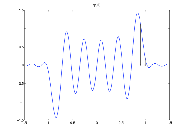
Figure 1: The function $\psi_{n}(t)$ for $c=20$ and $n=9$. Since $\chi_{n}\approx 325.42<c^{2}$, the behavior is as asserted in (74) of Theorem 16. The points $\sqrt{\chi_{n}}/c\approx 0.90197$ and $1$ are marked with asterisks. The eigenvalue $\left|\lambda_{n}\right|\approx 0.55978$ is relatively large, and the oscillations of $\psi_{n}$ outside $(-1,1)$ have small magnitude. Compare to Figure 2. Corresponds to Experiment 1.

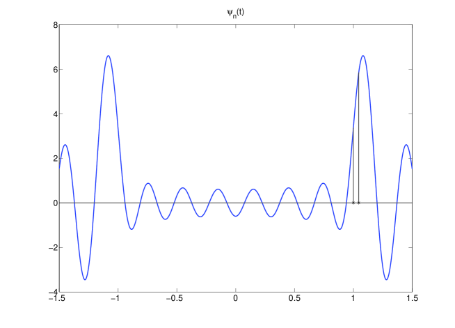
Figure 2: The function $\psi_{n}(t)$ for $c=20$ and $n=14$. Since $\chi_{n}\approx 437.36>c^{2}$, the behavior is as asserted in (75) of Theorem 16. The points $1$ and $\sqrt{\chi_{n}}/c\approx 1.0457$ are marked with asterisks. Observe that $\left|\lambda_{n}\right|\approx 0.12564$, and the oscillations of $\psi_{n}$ outside $(-1,1)$ have relatively large magnitude (of order $\left|\lambda_{n}\right|^{-1}$). Compare to Figure 1. Corresponds to Experiment 1.

$c$	$n$	$x_{1}-\sqrt{\chi_{n}}/c$	$\frac{\pi}{2c}\sqrt{\frac{x_{1}^{2}-1}{x_{1}^{2}-(\chi_{n}/c^{2})}}$	$(x_{1}-\sqrt{\chi_{n}}/c)\cdot\frac{2c}{\pi}\sqrt{\frac{x_{1}^{2}-(\chi_{n}/c^{2})}{x_{1}^{2}-1}}$
10	15	0.46561E+00	0.22542E+00	0.20655E+01
10	19	0.51090E+00	0.24279E+00	0.21043E+01
10	24	0.55570E+00	0.26055E+00	0.21328E+01
100	76	0.49260E-01	0.23935E-01	0.20581E+01
100	84	0.57274E-01	0.27070E-01	0.21158E+01
100	92	0.63570E-01	0.29602E-01	0.21475E+01
1000	652	0.52819E-02	0.23016E-02	0.22949E+01
1000	664	0.56889E-02	0.27295E-02	0.20843E+01
1000	676	0.63367E-02	0.30338E-02	0.20887E+01

Table 1: The relation between the left-hand side and the right-hand side of the inequality (228) of Theorem 31. For each value of the band limit $c$, the three values of $n$ are chosen such that $|\lambda_{n}|\approx 10^{-5},10^{-9},10^{-13}$, respectively. Corresponds to Experiment 2.

Experiment 2.

In the following numerical experiment, we illustrate Theorem 31 in Section 4.1.1. We proceed as follows. For each of the three values of band limit $c$ (namely, $c=10,100,1000$), we pick three values of the prolate index $n$. The values of $n$ are chosen to satisfy $n>2c/\pi$ (which implies that $\chi_{n}>c^{2}$, due to Theorem 4 in Section 2.1). Then, we evaluate the eigenvalue $\chi_{n}$ of the ODE (48) of Section 2.1, by using the algorithm of Section 5.1. Also, we evaluate the minimal root $x_{1}$ of $\psi_{n}$ in $(1,\infty)$ (see Theorem 29 in Section 4.1.1), by using the algorithm of Section 5.5.3.

The results of this experiment are displayed in Table 1. This table has the following structure. The first two columns contain the band limit $c$ and PSWF index $n$. The third column contains the difference between the $x_{1}$ and the special point $\sqrt{\chi_{n}}/c$ (see Theorem 29 in Section 4.1.1). This difference is the left-hand side of the inequality (228) of Theorem 31. On the other hand, the fourth column contains the right-hand side of (228) (a lower bound on this difference). The last column contains the ratio of the value in the third column to the value in the fourth column.

We observe that the value in the fourth column is smaller than the value in the third column roughly by a factor of 2, for all the choices of $c,n$. In other words, the lower bound on $x_{1}-\sqrt{\chi_{n}}/c$, provided by Theorem 31, is rather inaccurate, but is of correct order.

$k$	$x_{k+1}-x_{k}$	$\frac{\pi\left(x_{k}^{2}-1\right)}{\sqrt{1+c^{2}\left(x_{k}^{2}-1\right)^{2}}}$	$\frac{\pi}{c}\sqrt{\frac{x_{k}^{2}-1}{x_{k}^{2}-(\chi_{n}/c^{2})}}$	lower error	upper error
1	0.51496E-01	0.31410E-01	0.58023E-01	0.39005E+00	0.12676E+00
2	0.45166E-01	0.31412E-01	0.47546E-01	0.30452E+00	0.52703E-01
3	0.42078E-01	0.31413E-01	0.43379E-01	0.25345E+00	0.30936E-01
4	0.40179E-01	0.31414E-01	0.41019E-01	0.21815E+00	0.20908E-01
5	0.38872E-01	0.31414E-01	0.39466E-01	0.19185E+00	0.15285E-01
6	0.37908E-01	0.31415E-01	0.38354E-01	0.17129E+00	0.11754E-01
7	0.37164E-01	0.31415E-01	0.37512E-01	0.15470E+00	0.93670E-02
8	0.36570E-01	0.31415E-01	0.36851E-01	0.14097E+00	0.76646E-02
9	0.36084E-01	0.31415E-01	0.36315E-01	0.12939E+00	0.64016E-02
10	0.35678E-01	0.31415E-01	0.35872E-01	0.11949E+00	0.54352E-02
11	0.35334E-01	0.31415E-01	0.35499E-01	0.11090E+00	0.46772E-02
12	0.35038E-01	0.31415E-01	0.35180E-01	0.10338E+00	0.40703E-02
13	0.34780E-01	0.31415E-01	0.34905E-01	0.96745E-01	0.35761E-02
14	0.34554E-01	0.31416E-01	0.34664E-01	0.90835E-01	0.31677E-02
15	0.34354E-01	0.31416E-01	0.34451E-01	0.85540E-01	0.28261E-02
16	0.34176E-01	0.31416E-01	0.34263E-01	0.80768E-01	0.25372E-02
17	0.34016E-01	0.31416E-01	0.34094E-01	0.76444E-01	0.22905E-02
18	0.33872E-01	0.31416E-01	0.33942E-01	0.72510E-01	0.20780E-02
19	0.33741E-01	0.31416E-01	0.33805E-01	0.68913E-01	0.18937E-02

Table 2: Illustration of Theorem 32 with $c=100$ and $n=90$. $|\lambda_{n}|\approx 10^{-10}$. Corresponds to Experiment 3.

$k$	$x_{k+1}-x_{k}$	$\frac{\pi\left(x_{k}^{2}-1\right)}{\sqrt{1+c^{2}\left(x_{k}^{2}-1\right)^{2}}}$	$\frac{\pi}{c}\sqrt{\frac{x_{k}^{2}-1}{x_{k}^{2}-(\chi_{n}/c^{2})}}$	lower error	upper error
1	0.59672E-01	0.31414E-01	0.68077E-01	0.47355E+00	0.14086E+00
2	0.51323E-01	0.31415E-01	0.54472E-01	0.38790E+00	0.61363E-01
3	0.47161E-01	0.31415E-01	0.48918E-01	0.33387E+00	0.37253E-01
4	0.44558E-01	0.31415E-01	0.45710E-01	0.29496E+00	0.25858E-01
5	0.42740E-01	0.31415E-01	0.43566E-01	0.26496E+00	0.19329E-01
6	0.41383E-01	0.31415E-01	0.42010E-01	0.24087E+00	0.15150E-01
7	0.40325E-01	0.31415E-01	0.40820E-01	0.22094E+00	0.12275E-01
8	0.39472E-01	0.31416E-01	0.39874E-01	0.20410E+00	0.10193E-01
9	0.38767E-01	0.31416E-01	0.39102E-01	0.18964E+00	0.86267E-02
10	0.38174E-01	0.31416E-01	0.38457E-01	0.17705E+00	0.74127E-02
11	0.37667E-01	0.31416E-01	0.37910E-01	0.16597E+00	0.64491E-02
12	0.37229E-01	0.31416E-01	0.37440E-01	0.15614E+00	0.56691E-02
13	0.36845E-01	0.31416E-01	0.37030E-01	0.14735E+00	0.50273E-02
14	0.36506E-01	0.31416E-01	0.36670E-01	0.13943E+00	0.44920E-02
15	0.36204E-01	0.31416E-01	0.36350E-01	0.13225E+00	0.40401E-02
16	0.35933E-01	0.31416E-01	0.36065E-01	0.12572E+00	0.36546E-02
17	0.35690E-01	0.31416E-01	0.35808E-01	0.11975E+00	0.33228E-02
18	0.35469E-01	0.31416E-01	0.35576E-01	0.11426E+00	0.30349E-02
19	0.35267E-01	0.31416E-01	0.35365E-01	0.10921E+00	0.27833E-02

Table 3: Illustration of Theorem 32 with $c=100$ and $n=110$. $|\lambda_{n}|\approx 10^{-25}$. Corresponds to Experiment 3.

Experiment 3.

In the following numerical experiment, we illustrate Theorem 32 in Section 4.1.1. We proceed as follows. We choose the band limit $c$ and the prolate index $n$. For each such choice, we compute the first 20 roots $x_{1},\dots,x_{20}$ of $\psi_{n}$ in $(1,\infty)$, using the algorithm of Section 5.5.3. Also, for each $k=1,\dots,19$, we compute the upper and lower bound on $x_{k+1}-x_{k}$, established in Theorem 32.

The results of the experiment are displayed in Tables 2, 3, that correspond to $c=100$ and $n=90,110$, respectively. These tables have the following structure. The first column contains the index $k$ of the root $x_{k}$ of $\psi_{n}$ in $(1,\infty)$. The second column contains the difference between two consecutive roots $x_{k+1}$ and $x_{k}$ of $\psi_{n}$ in $(1,\infty)$. The third and fourth columns contain, respectively, the lower and upper bound on $x_{k+1}-x_{k}$, as in (233) of Theorem 32. The last two columns contain the relative errors of these bounds.

We observe that the upper bound is more accurate in terms of relative error. Moreover, the relative accuracy of both bounds improves monotonically as $k$ grows. On the other hand, for a fixed $k$, the accuracy in Table 2 is slightly higher than that in Table 3, which suggests that the bounds worsen as $n$ grows. We also observe that the difference $x_{k+1}-x_{k}$ between two consecutive roots decreases monotonically to $\pi/c$, as $k$ grows (see (235) in Theorem 32 and Remark 7).

6.1.2 Illustration of Results from Section 4.2

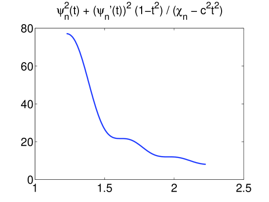
Figure 3: $Q(t)$ defined via (244), with $c=10$ and $n=8$. See Experiment 4.

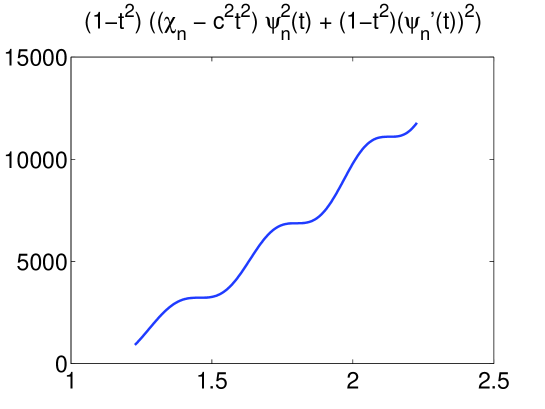
Figure 4: $\tilde{Q}(t)$ defined via (245), with $c=10$ and $n=8$. See Experiment 4.

Experiment 4.

In this experiment, we illustrate Theorem 34 in Section 4.2.1. We proceed as follows. We choose the band limit $c=10$ and the prolate index $n=8$. Then, we compute $\chi_{n}$ by using the algorithm of Section 5.1. Also, we evaluate $\psi_{n}$ and $\psi_{n}^{\prime}$ at 500 equispaced points in the interval

$$\left(\frac{\sqrt{\chi_{n}}+1}{c},\frac{\sqrt{\chi_{n}}+1}{c}+1\right).$$ (626)

For each such point $x$, we compute $Q(x)$ and $\tilde{Q}(x)$, where the functions $Q,\tilde{Q}$ are defined, respectively, via (244), (245) in Theorem 34.

In Figures 3, 4, we plot, respectively, $Q$ and $\tilde{Q}$ over the interval (626). We observe that, as expected, $Q$ is monotonically decreasing and $\tilde{Q}$ is monotonically increasing. On the other hand, we observe that the second derivative of each of $Q,\tilde{Q}$ does not have a constant sign in this interval.

$k$	$\left|\frac{\psi_{n}^{\prime}(x_{k+1})}{\psi_{n}^{\prime}(x_{k})}\right|$	$\frac{x_{k}^{2}-1}{x_{k+1}^{2}-1}$	$\sqrt{\frac{x_{k}^{2}-1}{c^{2}x_{k}^{2}-\chi_{n}}\cdot\frac{c^{2}x_{k+1}^{2}-\chi_{n}}{x_{k+1}^{2}-1}}$	lower error	upper error
1	0.93958E+00	0.74737E+00	0.11909E+01	0.20457E+00	0.26750E+00
2	0.93463E+00	0.81017E+00	0.10796E+01	0.13317E+00	0.15516E+00
3	0.93943E+00	0.84386E+00	0.10463E+01	0.10172E+00	0.11373E+00
4	0.94463E+00	0.86575E+00	0.10309E+01	0.83504E-01	0.91326E-01
5	0.94920E+00	0.88139E+00	0.10223E+01	0.71439E-01	0.77048E-01
6	0.95309E+00	0.89325E+00	0.10170E+01	0.62785E-01	0.67058E-01
7	0.95639E+00	0.90260E+00	0.10134E+01	0.56236E-01	0.59629E-01
8	0.95922E+00	0.91021E+00	0.10109E+01	0.51085E-01	0.53864E-01
9	0.96166E+00	0.91655E+00	0.10090E+01	0.46915E-01	0.49244E-01
10	0.96380E+00	0.92191E+00	0.10076E+01	0.43460E-01	0.45449E-01
11	0.96568E+00	0.92653E+00	0.10065E+01	0.40545E-01	0.42269E-01
12	0.96735E+00	0.93055E+00	0.10056E+01	0.38048E-01	0.39561E-01
13	0.96885E+00	0.93408E+00	0.10049E+01	0.35883E-01	0.37225E-01
14	0.97019E+00	0.93722E+00	0.10043E+01	0.33984E-01	0.35185E-01
15	0.97141E+00	0.94003E+00	0.10038E+01	0.32304E-01	0.33386E-01
16	0.97252E+00	0.94256E+00	0.10034E+01	0.30805E-01	0.31788E-01
17	0.97353E+00	0.94485E+00	0.10031E+01	0.29459E-01	0.30356E-01
18	0.97447E+00	0.94694E+00	0.10028E+01	0.28242E-01	0.29065E-01
19	0.97533E+00	0.94886E+00	0.10025E+01	0.27136E-01	0.27895E-01

Table 4: Illustration of Theorem 35, with $c=100$, $n=80$, $|\lambda_{n}|=\mbox{\text{\rm{0.58925E-07}}}$. See Experiment 5.

$k$	$\left|\frac{\psi_{n}^{\prime}(x_{k+1})}{\psi_{n}^{\prime}(x_{k})}\right|$	$\frac{x_{k}^{2}-1}{x_{k+1}^{2}-1}$	$\sqrt{\frac{x_{k}^{2}-1}{c^{2}x_{k}^{2}-\chi_{n}}\cdot\frac{c^{2}x_{k+1}^{2}-\chi_{n}}{x_{k+1}^{2}-1}}$	lower error	upper error
1	0.99507E+00	0.81420E+00	0.12260E+01	0.18177E+00	0.23205E+00
2	0.97042E+00	0.85769E+00	0.10994E+01	0.11618E+00	0.13292E+00
3	0.96628E+00	0.88122E+00	0.10600E+01	0.88030E-01	0.96998E-01
4	0.96620E+00	0.89669E+00	0.10413E+01	0.71944E-01	0.77728E-01
5	0.96726E+00	0.90789E+00	0.10306E+01	0.61380E-01	0.65503E-01
6	0.96863E+00	0.91647E+00	0.10238E+01	0.53843E-01	0.56971E-01
7	0.97004E+00	0.92332E+00	0.10192E+01	0.48159E-01	0.50637E-01
8	0.97139E+00	0.92894E+00	0.10158E+01	0.43700E-01	0.45725E-01
9	0.97265E+00	0.93365E+00	0.10133E+01	0.40096E-01	0.41791E-01
10	0.97382E+00	0.93768E+00	0.10114E+01	0.37115E-01	0.38560E-01
11	0.97490E+00	0.94116E+00	0.10099E+01	0.34603E-01	0.35854E-01
12	0.97588E+00	0.94421E+00	0.10086E+01	0.32453E-01	0.33550E-01
13	0.97679E+00	0.94691E+00	0.10076E+01	0.30590E-01	0.31562E-01
14	0.97763E+00	0.94932E+00	0.10068E+01	0.28957E-01	0.29826E-01
15	0.97840E+00	0.95148E+00	0.10061E+01	0.27514E-01	0.28297E-01
16	0.97912E+00	0.95344E+00	0.10055E+01	0.26228E-01	0.26938E-01
17	0.97978E+00	0.95522E+00	0.10050E+01	0.25073E-01	0.25721E-01
18	0.98040E+00	0.95684E+00	0.10045E+01	0.24030E-01	0.24624E-01
19	0.98098E+00	0.95834E+00	0.10042E+01	0.23082E-01	0.23630E-01

Table 5: Illustration of Theorem 35, $c=200$, $n=160$, $|\lambda_{n}|=\mbox{\text{\rm{0.17136E-13}}}$. See Experiment 5.

Experiment 5.

In the following experiment, we illustrate Theorem 35 in Section 4.2.1. We proceed as follows. We choose, more or less arbitrarily, the band limit $c$ and the prolate index $n$. For each choice of $c,n$, we evaluate $\chi_{n}$ by using the algorithm of Section 5.1. Then, we evaluate the first 20 roots $x_{1},\dots,x_{20}$ of $\psi_{n}$ in $(1,\infty)$, by using the algorithm of Section 5.5.3 (in extended precision). For each such root $x_{k}$, we evaluate $\psi_{n}^{\prime}(x_{k})$ by using the algorithm of Section 5.5.2 (in extended precision).

We display the results of the experiment in Tables 4, 5, corresponding to $c=100$, $n=80$ and $c=200$, $n=160$, respectively. These tables have the following structure. The first column contains the index $k$ of the root $x_{k}$ of $\psi_{n}$ in $(1,\infty)$. The second column contains the absolute value of the ratio of $\psi_{n}^{\prime}(x_{k+1})$ to $\psi_{n}^{\prime}(x_{k})$. The third and fourth columns contain the lower and upper bound on that ratio, respectively, established in (254) of Theorem 35. The last two columns contain the relative errors of these bounds.

We observe that the ratio in the second column is always less than one. Moreover, it first decreases up to a certain $k$ and then increases as $k$ grows. Both bounds have roughly the same relative accuracy and become sharper as $k$ grows. Even for $k=1$ the errors are about $20\%$, while already at $k=7$ they drop to about $5\%$. We also observe (not shown in the tables) that the magnitude of $\left|\psi_{n}^{\prime}(x_{k})\right|$ is about $10^{8}$ for Table 4 and about $10^{15}$ for Table 5 (see also Experiment 6 below).

$k$	$\left|\psi_{n}^{\prime}(x_{k})\right|^{-1}$	$\frac{|\lambda_{n}|\left(x_{k}^{2}-1\right)^{3/4}}{\left(x_{k}^{2}-(\chi_{n}/c^{2})\right)^{1/4}|\psi_{n}(1)|\sqrt{2}}$	$\varepsilon_{k}$	$b_{c}\left(x_{k},\frac{\sqrt{\chi_{n}}}{c}\right)$
1	0.57349E-19	0.81518E-19	0.72340E-02	0.10181E+01
2	0.56895E-19	0.80550E-19	0.15530E-02	0.10106E+01
3	0.58182E-19	0.82319E-19	0.64593E-03	0.10081E+01
4	0.59907E-19	0.84743E-19	0.34935E-03	0.10067E+01
5	0.61785E-19	0.87390E-19	0.21744E-03	0.10059E+01
6	0.63718E-19	0.90120E-19	0.14767E-03	0.10052E+01
7	0.65667E-19	0.92874E-19	0.10641E-03	0.10048E+01
8	0.67615E-19	0.95627E-19	0.80051E-04	0.10044E+01
9	0.69553E-19	0.98367E-19	0.62211E-04	0.10041E+01
10	0.71477E-19	0.10109E-18	0.49596E-04	0.10039E+01
11	0.73385E-19	0.10379E-18	0.40358E-04	0.10036E+01
12	0.75277E-19	0.10646E-18	0.33400E-04	0.10035E+01
13	0.77154E-19	0.10911E-18	0.28034E-04	0.10033E+01
14	0.79015E-19	0.11175E-18	0.23815E-04	0.10032E+01
15	0.80861E-19	0.11436E-18	0.20441E-04	0.10030E+01
16	0.82693E-19	0.11695E-18	0.17703E-04	0.10029E+01
17	0.84511E-19	0.11952E-18	0.15453E-04	0.10028E+01
18	0.86317E-19	0.12207E-18	0.13584E-04	0.10027E+01
19	0.88112E-19	0.12461E-18	0.12015E-04	0.10026E+01

Table 6: Illustration of Theorem 41 with $c=100$, $n=100$. $\lambda_{n}=\mbox{\text{\rm{0.94419E-18}}}$. See Experiment 6.

$k$	$\left|\psi_{n}^{\prime}(x_{k})\right|^{-1}$	$\frac{|\lambda_{n}|\left(x_{k}^{2}-1\right)^{3/4}}{\left(x_{k}^{2}-(\chi_{n}/c^{2})\right)^{1/4}|\psi_{n}(1)|\sqrt{2}}$	$\varepsilon_{k}$	$b_{c}\left(x_{k},\frac{\sqrt{\chi_{n}}}{c}\right)$
1	0.10723E-23	0.15242E-23	0.72932E-02	0.10140E+01
2	0.10407E-23	0.14734E-23	0.15865E-02	0.10077E+01
3	0.10464E-23	0.14805E-23	0.67023E-03	0.10056E+01
4	0.10621E-23	0.15025E-23	0.36864E-03	0.10045E+01
5	0.10817E-23	0.15300E-23	0.23349E-03	0.10038E+01
6	0.11028E-23	0.15598E-23	0.16142E-03	0.10033E+01
7	0.11246E-23	0.15905E-23	0.11843E-03	0.10029E+01
8	0.11466E-23	0.16216E-23	0.90717E-04	0.10027E+01
9	0.11685E-23	0.16527E-23	0.71782E-04	0.10025E+01
10	0.11903E-23	0.16835E-23	0.58262E-04	0.10023E+01
11	0.12119E-23	0.17140E-23	0.48264E-04	0.10021E+01
12	0.12332E-23	0.17441E-23	0.40656E-04	0.10020E+01
13	0.12542E-23	0.17738E-23	0.34730E-04	0.10019E+01
14	0.12750E-23	0.18031E-23	0.30020E-04	0.10018E+01
15	0.12954E-23	0.18320E-23	0.26215E-04	0.10017E+01
16	0.13156E-23	0.18606E-23	0.23094E-04	0.10016E+01
17	0.13355E-23	0.18887E-23	0.20502E-04	0.10015E+01
18	0.13551E-23	0.19164E-23	0.18325E-04	0.10015E+01
19	0.13745E-23	0.19438E-23	0.16479E-04	0.10014E+01

Table 7: Illustration of Theorem 41 with $c=1000$, $n=700$. $\lambda_{n}=\mbox{\text{\rm{0.12446E-21}}}$. See Experiment 6.

Experiment 6

In this experiment, we illustrate Theorems 41, 42 in Section 4.2.2. We proceed as follows. We choose, more or less arbitrarily, the band limit $c$ and the prolate index $n$. For each such choice, we evaluate $\chi_{n}$ and $\lambda_{n}$, by using the algorithms of Sections 5.1, 5.2, respectively (in double precision). Then, we compute the first 20 roots $x_{1},\dots,x_{20}$ of $\psi_{n}$ in $(1,\infty)$, by using the algorithm of Section 5.5.3 (in extended precision). For each such root $x_{k}$, we evaluate $\psi_{n}^{\prime}(x_{k})$ by using the algorithm of Section 5.5.2 (in extended precision).

We display the results of the experiment in Tables 6, 7, corresponding to $c=100,n=100$ and $c=1000,n=700$, respectively. These tables have the following structure. The first column contains the index $k$ of the root $x_{k}$ of $\psi_{n}$ in $(1,\infty)$. The second column contains the reciprocal of $|\psi_{n}^{\prime}(x_{k})|$. The third column contains the quantity

$$\frac{|\lambda_{n}|\left(x_{k}^{2}-1\right)^{3/4}}{\left(x_{k}^{2}-(\chi_{n}/c^{2})\right)^{1/4}|\psi_{n}(1)|\sqrt{2}}$$ (627)

(see (306) in Theorem 41). The fourth column contains $\varepsilon_{k}$, defined via the formula

$$|\psi_{n}^{\prime}(x_{k})|=\frac{2\cdot|\psi_{n}(1)|\left(x_{k}^{2}-(\chi_{n}/c^{2})\right)^{1/4}}{|\lambda_{n}|\left(x_{k}^{2}-1\right)^{3/4}}\cdot(1+\varepsilon_{k})$$ (628)

(we observe that $\varepsilon_{k}$ in (628) is obtained via multiplying (627) by $|\psi_{n}^{\prime}(x_{k})|/\sqrt{2}$ and subtracting 1 from the result). The last column contains $b_{c}(x_{k},\sqrt{\chi_{n}}/c)$, defined via (266) of Definition 1 in Section 4.2.2.

According to Theorem 41, the product of the values in the third and fifth columns is an upper bound on $|\psi_{n}^{\prime}(x_{k})|^{-1}$ (the second column). However, (627) alone (the third column) already overestimates $|\psi_{n}^{\prime}(x_{k})|^{-1}$ by roughly $\sqrt{2}$. We also observe (see the fourth column) that the parameter $\varepsilon_{k}$, defined via (628), is fairly small, and decreases as $k$ grows. According to Theorems 49, 51 in Section 4.3.2, we expect $\varepsilon_{k}$ to tend to zero as $k$ grows to $\infty$, since

$$\frac{2\cdot|\psi_{n}(1)|\left(x_{k}^{2}-(\chi_{n}/c^{2})\right)^{1/4}}{|\lambda_{n}|\left(x_{k}^{2}-1\right)^{3/4}}\sim\frac{2\cdot|\psi_{n}(1)|}{|\lambda_{n}\cdot x_{k}|},\quad k\to\infty.$$ (629)

On the other hand, the fact that $\varepsilon_{k}\approx 10^{-4}$ already for $k=7$ is somewhat surprising. In other words, the left hand side of (629) is a fairly tight estimate of $|\psi_{n}^{\prime}(x_{k})|$, even for small $k$.

We also observe that $b_{c}(x_{k},\sqrt{\chi_{n}}/c)$ (see the last column) is very close to $1$ even for $k=1$, and becomes even closer to $1$ as $k$ increases. In other words, the upper bound $e^{1/4}\approx 1.284$ on this quantity (see Theorem 42 in Section 4.2.2) is somewhat overcautious.

6.1.3 Illustration of Results from Section 4.3

$k$	$\left|\sum_{j=k}^{k+1}\frac{1}{\left(1-x_{j}\right)\psi_{n}^{\prime}(x_{j})}\right|$	$e^{1/4}\cdot\left|\lambda_{n}\right|\cdot\int_{x}^{y}\frac{(z+1)^{2}\;dz}{\left(z^{2}-\left(\chi_{n}/c^{2}\right)\right)^{3/2}}$	ratio
1	0.29442E-19	0.31341E-17	0.10645E+03
3	0.99172E-20	0.85727E-18	0.86442E+02
5	0.57139E-20	0.46271E-18	0.80980E+02
7	0.39054E-20	0.30749E-18	0.78735E+02
9	0.29098E-20	0.22656E-18	0.77861E+02
11	0.22851E-20	0.17760E-18	0.77720E+02
13	0.18596E-20	0.14509E-18	0.78022E+02
15	0.15530E-20	0.12209E-18	0.78614E+02
17	0.13226E-20	0.10503E-18	0.79407E+02
19	0.11441E-20	0.91920E-19	0.80345E+02
21	0.10021E-20	0.81564E-19	0.81393E+02
23	0.88694E-21	0.73193E-19	0.82524E+02
25	0.79193E-21	0.66300E-19	0.83720E+02
27	0.71242E-21	0.60534E-19	0.84969E+02
29	0.64507E-21	0.55645E-19	0.86261E+02
31	0.58742E-21	0.51451E-19	0.87588E+02
33	0.53762E-21	0.47818E-19	0.88944E+02
35	0.49425E-21	0.44643E-19	0.90325E+02
37	0.45620E-21	0.41846E-19	0.91727E+02
39	0.42261E-21	0.39365E-19	0.93147E+02

Table 8: Illustration of Theorem 44 with $c=n=100$. $\lambda_{n}=\mbox{\text{\rm{0.94419E-18}}}$. See Experiment 7.

Experiment 7.

In this experiment, we illustrate Theorem 44 in Section 4.3.1. We proceed as follows. We choose the band limit and the prolate index to be, respectively, $c=100$ and $n=100$. We evaluate $\chi_{n}$ and $\lambda_{n}$, by using the algorithms of Sections 5.1, 5.2, respectively (in double precision). Then, we compute the first 40 roots $x_{1},\dots,x_{40}$ of $\psi_{n}$ in $(1,\infty)$, by using the algorithm of Section 5.5.3 (in extended precision). For each such root $x_{k}$, we evaluate $\psi_{n}^{\prime}(x_{k})$ by using the algorithm of Section 5.5.2 (in extended precision).

For each $k=1,3,5,\dots,39$, we evaluate

$$\max_{-1\leq t\leq 1}\left|\frac{1}{(t-x_{k})\cdot\psi_{n}^{\prime}(x_{k})}+\frac{1}{(t-x_{k+1})\cdot\psi_{n}^{\prime}(x_{k+1})}\right|$$ (630)

(it turns out that the maximum is attained at $t=1$.) Then, we evaluate the upper bound on (630), provided by Theorem 44.

We display the results of the experiment in Table 8. The first column contains the index $k$ of the root $x_{k}$ of $\psi_{n}$ in $(1,\infty)$. The second column contains the quantity (630). The third column contains the upper bound on (630), provided by (314) in Theorem 44. The last column contains the ratio of the third column to the second column.

We observe that the quantity (630) (in the second column) decreases with $k$. On the other hand, the bound on (630) (in the third column) gets tighter as $k$ increases from 1 to 11, and then deteriorates, as $k$ increases further on, roughly linearly in $k$. The latter observation is not surprising, since

$$|\lambda_{n}|\cdot\int_{x}^{y}\frac{(z+1)^{2}\;dz}{\left(z^{2}-\left(\chi_{n}/c^{2}\right)\right)^{3/2}}\sim\frac{\pi\cdot|\lambda_{n}|}{c\cdot x_{k}},\quad k\to\infty,$$ (631)

due to Theorem 32 in Section 4.1.1, while, for sufficiently large $k$,

$$\left|\frac{1}{(t-x_{k})\cdot\psi_{n}^{\prime}(x_{k})}+\frac{1}{(t-x_{k+1})\cdot\psi_{n}^{\prime}(x_{k+1})}\right|\leq\frac{20\cdot\pi\cdot|\lambda_{n}|}{x_{k}^{2}},$$ (632)

due to Theorem 52 in Section 4.3.2. In other words, the upper bound on (630), provided by Theorem 44, is of a wrong order ($O(x_{k}^{-1})$ instead of $O(x_{k}^{-2})$). In particular, it can be used only to bound the head of the convergent series

$$\left|\sum_{k=1}^{\infty}\frac{1}{(t-x_{k})\cdot\psi_{n}^{\prime}(x_{k})}\right|.$$ (633)

Of course, this is precisely how Theorem 44 is used (see the proof of Theorem 45 in Section 4.3.1 and the proof of Theorem 53 in Section 4.3.3).

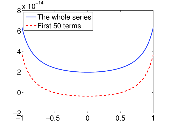
Figure 5: Illustration of Theorems 58 with $c=100$, $n=80$. $|\lambda_{n}|=\mbox{\text{\rm{0.58925E-07}}}$.

$c$	$n$	$\|I\|_{\infty}$	$\left|\lambda_{n}\right|$	$\left|\lambda_{n}\right|/\|I\|_{\infty}$	$I_{\max}$
100	80	0.99408E-08	0.58925E-07	0.59276E+01	0.55502E+03
100	81	0.28195E-08	0.19431E-07	0.68914E+01	0.58207E+03
100	90	0.63405E-13	0.45487E-12	0.71741E+01	0.84186E+03
100	91	0.14648E-13	0.12985E-12	0.88645E+01	0.87239E+03
200	146	0.57204E-08	0.32856E-07	0.57436E+01	0.62129E+03
200	147	0.19902E-08	0.12477E-07	0.62691E+01	0.64480E+03
200	158	0.21537E-13	0.15123E-12	0.70219E+01	0.91959E+03
200	159	0.64626E-14	0.51123E-13	0.79107E+01	0.94591E+03
400	274	0.15108E-07	0.80630E-07	0.53369E+01	0.67438E+03
400	275	0.61774E-08	0.34713E-07	0.56193E+01	0.69478E+03
400	288	0.47053E-13	0.31193E-12	0.66293E+01	0.97598E+03
400	289	0.17000E-13	0.12189E-12	0.71703E+01	0.99872E+03
800	530	0.18269E-07	0.91984E-07	0.50351E+01	0.77801E+03
800	531	0.83405E-08	0.43433E-07	0.52075E+01	0.79612E+03
800	546	0.46822E-13	0.29701E-12	0.63434E+01	0.10833E+04
800	547	0.19631E-13	0.12945E-12	0.65942E+01	0.11033E+04

Table 9: Illustration of Theorem 58. See Experiment 8.

Experiment 8.

In this experiment, we illustrate Theorem 58 in Section 4.3.3. We proceed as follows. We choose, more or less arbitrarily, the band limit $c$ and the prolate index $n$. Then, we evaluate $\chi_{n}$ and $\lambda_{n}$, by using the algorithms of Section 5.1, 5.2, respectively (in double precision). Next, we find the roots $t_{1},\dots,t_{n}$ of $\psi_{n}$ in the interval $(-1,1)$, by using the algorithm of Section 5.3 (in double precision). For each root $t_{i}$, we compute $\psi_{n}^{\prime}(t_{i})$.

Suppose now that the function $I:[-1,1]\to\mathbb{R}$ is defined via (417) in Theorem 56. We evaluate $I$ at $3\cdot(n+1)$ points $z_{1},\dots,z_{3(n+1)}$ in the interval $[-1,1]$. The points are chosen in such a way that, if $t_{k}<z_{j}<t_{k+1}$ for some $j,k$, then

$$\frac{1}{3}\leq\frac{z_{j}-t_{k}}{t_{k+1}-z_{j}}\leq 3.$$ (634)

In other words, no point $z_{j}$ is “too close” to any root of $\psi_{n}$ in $(-1,1)$. For each $j=1,\dots,3\cdot(n+1)$, we evaluate $I(z_{j})$ in extended precision.

Remark 25.

For each $-1\leq t\leq 1$, we expect $I(t)$ to be of order $|\lambda_{n}|$, due to Theorems 56, 58. On the other hand, suppose that $-1\leq t\leq 1$, and $t_{k}$ is the closest root of $\psi_{n}$ to $t$. Then,

$$\frac{1}{\psi_{n}(t)}=\frac{1}{(t-t_{k})\cdot\psi_{n}^{\prime}(t_{k})}+O(1).$$ (635)

Therefore, in the evaluation of $\psi_{n}(t)$, we expect to lose roughly

$$\log_{10}\left(\frac{1}{|\psi_{n}^{\prime}(t_{k})\cdot(t-t_{k})\cdot\lambda_{n}|}\right)$$ (636)

decimal digits. In other words, this calculation is rather inaccurate. However, since we need it only to illustrate the analysis, we were satisfied when we got at least two decimal digits, and did not make any attempts to enhance the accuracy.

On the other hand, we compute the first 50 roots $x_{1},\dots,x_{50}$ of $\psi_{n}$ in $(1,\infty)$, and, for each such root $x_{j}$, we evaluate $\psi_{n}^{\prime}(x_{j})$. These calculations are based on the algorithms of Sections 5.5.2, 5.5.3. Then, for each $z_{j}$, we evaluate the sum

$$I_{50}(z_{j})=\sum_{k=1}^{50}\left(\frac{1}{\psi_{n}^{\prime}(x_{k})\cdot(z_{j}-x_{k})}+\frac{1}{\psi_{n}^{\prime}(-x_{k})\cdot(z_{j}+x_{k})}\right).$$ (637)

We display the results of the experiment in Figures 5, 6, for $c=100$, $n=90$ and $c=100$, $n=91$, respectively. On each of these figures, we plot the function $I$, defined via (417) in Theorem 56 (blue solid line) and the function $I_{50}$, defined via (637) (red dashed line).

We observe that, in both figures, the maximum of both $I$ and $I_{50}$ is attained at the end points of the interval. Also, we observe that the values of $I$ and $I_{50}$ are of order $|\lambda_{n}|$, as expected; also, the functions appear, at least by eye, to be well approximated by polynomials of order up to 3. In other words, the reciprocal of $\psi_{n}$ seems to be approximated up to an error of order $|\lambda_{n}|$ by a rational function with $n$ poles, as asserted in Theorems 56, 58.

We display additional results of this experiment in Table 9. This table has the following structure. The first and second column contain the band limit $c$ and the prolate index $n$, respectively. The third column contains the maximum of the absolute value of the function $I$ in the interval $[-1,1]$, i.e.

$$\|I\|_{\infty}=\max\left\{|I(t)|\;:\;-1\leq t\leq 1\right\},$$ (638)

where $I$ is defined via (417) in Theorem 56. The fourth column contains $|\lambda_{n}|$. The fifth column contains the ratio $|\lambda_{n}|/\|I\|_{\infty}$. The last column contains $I_{\max}$, defined via (419) in Theorem 56.

We make the following observations from Table 9. First, $|\lambda_{n}|$ alone is already an upper bound on $\|I\|_{\infty}$. Moreover, for a fixed band limit $c$, the ratio $|\lambda_{n}|/\|I\|_{\infty}$ increases as $n$ grows. For all the values of $c,n$ in Table 9, this ratio varies between 5 and 9. On the other hand, $I_{\max}$ varies between 500 and 1000. Moreover, $I_{\max}$ increases with $n$, for each fixed band limit $c$. In other words, the upper bound $|\lambda_{n}|\cdot I_{\max}$ on $\|I\|_{\infty}$, established in Theorem 56, deteriorates as $n$ increases. Moreover, the factor $I_{\max}$ in (418) of Theorem 56 appears to be unnecessary. The main source of inaccuracy is Theorem 44 in Section 4.3.1, which provides a relatively poor upper bound on the expressions of the form (637) (see Figures 5, 6 and Experiment 7 above).

Nevertheless, due to the fast decay of $|\lambda_{n}|$ with $n$, the estimates of Theorem 56, albeit somewhat loose, are sufficient for the purposes of this paper (see the analysis of the quadrature error in Section 4.4, and also Experiment 14 in Section 6.2.1 below).

6.1.4 Illustration of Results from Section 4.4

Experiment 9.

In this numerical experiment, we illustrate Theorem 59 in Section 4.4.1. We proceed as follows. We choose, more or less arbitrarily, the band limit $c$, the prolate index $n$ and the root index $1\leq j\leq n$. Then, we evaluate $\lambda_{n}$ and the roots $t_{1},\dots,t_{n}$ of $\psi_{n}$ in $(-1,1)$, by using the algorithms of Sections 5.2, 5.3, respectively. We use $10\cdot n$ Gaussian nodes to evaluate

$$A_{n,j}=\int_{-1}^{1}\frac{\psi_{n}(t)\;dt}{t-t_{j}}$$ (639)

and

$$B_{n,j}=ic\lambda_{n}\cdot\Psi_{n}(1,t_{j}),$$ (640)

where $\Psi_{n}(1,t_{j})$ is defined via (437) in Theorem 59. We observe that $A_{n,j}$ and $B_{n,j}$ appear on the right-hand side of (436) in Theorem 59.

Next, for each integer $m=0,1,\dots,n-1$, we use the same Gaussian quadrature to evaluate

$$\int_{-1}^{1}\frac{\psi_{n}(t)\cdot\psi_{m}(t)\;dt}{t-t_{j}}.$$ (641)

In addition, for each integer $m=0,1,\dots,n-1$, we compute

$$\frac{|\lambda_{m}|^{2}\cdot\psi_{m}(t_{j})}{|\lambda_{m}|^{2}-|\lambda_{n}|^{2}},$$ (642)

by using the algorithms of Sections 5.1, 5.2. All the calculations are carried out in double precision.

$c$	$n$	$j$	$|\lambda_{n}|$	$A_{n,j}$	$B_{n,j}$
10	20	13	0.11487E-09	-.25341E+01	-.69171E-11
500	340	226	0.27418E-09	-.19569E+01	-.17690E-09

Table 10: Illustration of Theorem 59. See Experiment 9.

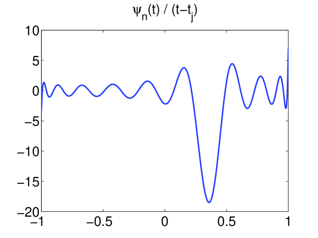
Figure 7: The graph of $\psi_{n}(t)/(t-t_{j})$ with $c=10$, $n=20$ and $j=13$. Corresponds to Table 11. See Experiment 9.

$m$	$\int_{-1}^{1}\frac{\psi_{n}(t)\psi_{m}(t)dt}{t-t_{j}}$	$\frac{\left|\lambda_{m}\right|^{2}\psi_{m}(t_{j})}{\left|\lambda_{m}\right|^{2}-\left|\lambda_{n}\right|^{2}}$	$E_{m}$
0	-.18363E+01	0.72463E+00	-.15543E-14
1	-.28929E+01	0.11416E+01	-.53291E-14
2	-.18299E+01	0.72208E+00	-.51070E-14
3	0.73457E+00	-.28987E+00	0.12212E-14
4	0.19270E+01	-.76041E+00	0.37748E-14
5	0.40316E+00	-.15909E+00	0.21094E-14
6	-.14464E+01	0.57078E+00	-.22204E-14
7	-.10263E+01	0.40498E+00	0.10658E-13
8	0.11062E+01	-.43654E+00	0.95479E-14
9	0.17030E+01	-.67204E+00	0.99920E-14
10	-.23035E+00	0.90899E-01	-.26645E-14
11	-.19061E+01	0.75217E+00	-.44409E-15
12	-.91510E+00	0.36111E+00	0.16653E-14
13	0.13774E+01	-.54355E+00	0.11990E-13
14	0.18002E+01	-.71037E+00	0.37748E-14
15	-.23786E+00	0.93863E-01	-.97422E-14
16	-.19723E+01	0.77830E+00	-.11546E-13
17	-.10566E+01	0.41697E+00	-.15987E-13
18	0.12849E+01	-.50705E+00	-.19984E-14
19	0.19509E+01	-.76986E+00	-.42188E-14

Table 11: Illustration of Theorem 59 with $c=10$, $n=20$ and $j=13$. See Experiment 9.

$m$	$\int_{-1}^{1}\frac{\psi_{n}(t)\psi_{m}(t)dt}{t-t_{j}}$	$\frac{\left|\lambda_{m}\right|^{2}\psi_{m}(t_{j})}{\left|\lambda_{m}\right|^{2}-\left|\lambda_{n}\right|^{2}}$	$E_{m}$
0	0.60926E-12	0.31814E-12	0.33872E-15
20	0.43712E-01	0.22813E-01	0.52666E-14
40	-.32804E+01	-.17120E+01	-.84377E-13
60	0.85749E+00	0.44751E+00	-.60729E-13
80	-.14190E+01	-.74055E+00	-.91926E-13
100	0.84651E+00	0.44178E+00	-.28089E-13
120	0.35414E+00	0.18482E+00	0.47351E-13
140	0.53788E+00	0.28071E+00	-.21316E-13
160	-.17111E+01	-.89302E+00	-.35749E-13
180	-.93523E+00	-.48808E+00	0.31863E-13
200	-.30219E+00	-.15771E+00	0.48406E-13
220	-.51322E+00	-.26784E+00	0.45852E-13
240	-.12216E+01	-.63753E+00	-.11546E-13
260	-.10503E+01	-.54811E+00	-.82379E-13
280	0.93142E+00	0.48609E+00	0.84377E-14
300	-.55310E-02	-.28865E-02	0.50818E-13
320	0.11601E+00	0.60544E-01	-.13105E-12
339	0.14218E+01	0.74200E+00	-.94369E-13

Table 12: Illustration of Theorem 59 with $c=500$, $n=340$ and $j=226$. See Experiment 9.

We display the results of the experiment in Figure 7 and Tables 11, 12. In Figure 7, we plot the function $\psi_{n}(t)/(t-t_{j})$, corresponding to $c=10$, $n=20$, and $j=13$, over the interval $(-1,1)$. We observe that this function has $n-1$ roots in $(-1,1)$: all the roots of $\psi_{n}$ except for $t_{j}$. Obviously, the value of this function at $t_{j}$ is $\psi_{n}^{\prime}(t_{j})$.

In Tables 10, 11, 12, we display the results of the experiment, corresponding to $c=10$, $n=20$, $j=13$ and $c=500$, $n=340$ and $j=226$, respectively. Table 10 contains the values of the parameters $c,n,j$, as well as the quantities $A_{n,j}$, $B_{n,j}$, defined, respectively, via (639), (640) above. Tables 11, 12 have the following structure. The first column contains the parameter $m$ (an integer between 0 and $n-1$). The second column contains (641) (the left-hand side of (436) in Theorem 59); in other words, this is the inner product of $\psi_{n}(t)/(t-t_{j})$ with $\psi_{m}$. The third column contains (642) (appears on the right-hand side of (436)). The last column contains the absolute error $E_{m}$ of the calculation of (642), defined via

$$E_{m}=\int_{-1}^{1}\frac{\psi_{n}(t)\cdot\psi_{m}(t)\;dt}{t-t_{j}}-\frac{|\lambda_{m}|^{2}\cdot\psi_{m}(t_{j})}{|\lambda_{m}|^{2}-|\lambda_{n}|^{2}}\cdot(A_{n,j}+B_{n,j})$$ (643)

(obviously, $E_{m}$ would be equal to zero in exact arithmetics, due to Theorem 59).

We make the following observations from Tables 10, 11, 12. As expected, $A_{n,j}$ is significantly larger than $B_{n,j}$ (by a factor of order $|\lambda_{n}|^{-1}$). In other words,

$$\int_{-1}^{1}\frac{\psi_{n}(t)\cdot\psi_{m}(t)\;dt}{t-t_{j}}=\frac{|\lambda_{m}|^{2}\cdot\psi_{m}(t_{j})}{|\lambda_{m}|^{2}-|\lambda_{n}|^{2}}\cdot\int_{-1}^{1}\frac{\psi_{n}(t)\;dt}{t-t_{j}}\cdot\left(1+O\left(|\lambda_{n}|\right)\right)$$ (644)

(see Theorem 59 and (639), (640), (641), (642) above). Also, in each of Tables 11, 12, all the quantities in the second and third column are roughly of the same order of magnitude (except for the first row in Table 12). We also observe that the numerical evaluations of the left-hand side and the right-hand side of (436) in Theorem 59 agree up to an absolute error of order $\approx 10^{-14}$.

$c$	$n$	$|\lambda_{n}|$	$|P_{n,n-2}|$
1000	670	0.93659E-11	0.49177E-03
1000	690	0.73056E-18	0.43907E-03
1000	710	0.15947E-25	0.40076E-03

Table 13: Illustration of Theorem 61. Corresponds to Figure 8.

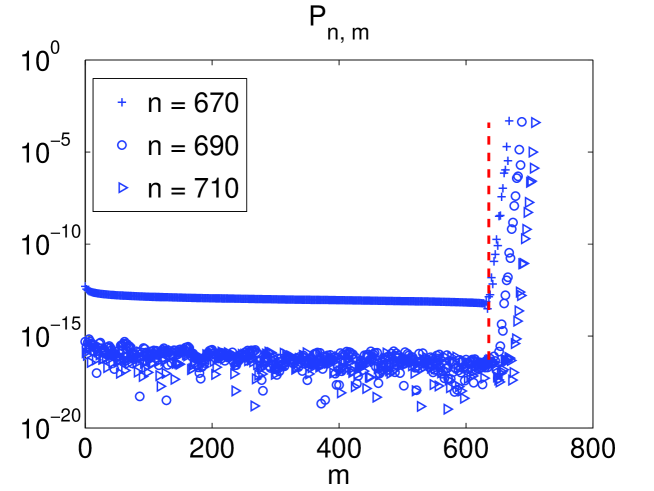
Figure 8: Plot of $P_{n,m}$ (448) with $c=1000$ and $n=670$ (crosses), $n=690$ (circles), $n=710$ (triangles). The value $m=2c/\pi$ is marked with a dashed line. See Experiment 10.

Experiment 10.

In this experiment, we illustrate Theorem 61 in Section 4.4.2. We proceed as follows. We choose, more or less arbitrarily, the band limit $c$ and the prolate index $n$. Then, we evaluate $\lambda_{n}$, using the algorithm of Section 5.2 (in double precision). Next, for each integer $0\leq m\leq n-1$, we evaluate $P_{n,m}$, defined via (448) in Theorem 60 in Section 4.4.2, by using the algorithms of Sections 5.1, 5.3 (in double precision). We observe that, due to Corollary 4 in Section 4.4.2, it suffices to consider only even values of $m$ (since $P_{n,m}=0$ if $m$ is odd).

$c$	$n$	$\left|\lambda_{n}\right|$	$\underset{0\leq m<n}{\max}|P_{n,m}|$	$c\cdot\underset{0\leq m<n}{\max}|P_{n,m}|$
50	47	0.26917E-07	0.81444E-02	0.40722E+00
50	53	0.72096E-11	0.72290E-02	0.36145E+00
50	57	0.19830E-13	0.67353E-02	0.33676E+00
100	81	0.19431E-07	0.48065E-02	0.48065E+00
100	87	0.18068E-10	0.44412E-02	0.44412E+00
100	93	0.10185E-13	0.41418E-02	0.41418E+00
250	179	0.18854E-07	0.22730E-02	0.56825E+00
250	186	0.22556E-10	0.14014E-02	0.35035E+00
250	193	0.17851E-13	0.20475E-02	0.51188E+00
500	339	0.40938E-07	0.12600E-02	0.63000E+00
500	348	0.20575E-10	0.85073E-03	0.42537E+00
500	355	0.39965E-13	0.11550E-02	0.57751E+00
1000	659	0.38241E-07	0.68143E-03	0.68143E+00
1000	668	0.44256E-10	0.49838E-03	0.49838E+00
1000	677	0.35933E-13	0.63339E-03	0.63339E+00
2000	1297	0.41740E-07	0.36453E-03	0.72906E+00
2000	1307	0.47570E-10	0.35192E-03	0.70385E+00
2000	1317	0.39064E-13	0.34212E-03	0.68424E+00
4000	2572	0.33682E-07	0.16247E-03	0.64987E+00
4000	2583	0.37417E-10	0.18703E-03	0.74813E+00
4000	2594	0.30728E-13	0.14902E-03	0.59608E+00

Table 14: Illustration of Theorem 61. See Experiment 10.

We display the results of the experiment in Tables 13, 14 and in Figure 8. In Figure 8, we plot $|P_{n,m}|$ as a function of even integer $m$ on the logarithmic scale for $c=1000$ and three choices of $n$, namely, $n=670$ (pluses), $n=690$ (circles), and $n=710$ (triangles). The value $2c/\pi$ is marked with a red dashed line. In Table 13, we display the quantities $|\lambda_{n}|$ and $|P_{n,n-2}|$, corresponding to Figure 8.

We make the following observations from Figure 8, Table 13 and some additional numerical experiments. First, $|P_{n,m}|<|\lambda_{n}|$ for all $m<2c/\pi$ (obviously, in Figure 8 we see this phenomenon only for $n=670$, since the calculations are carried out in double precision; for $n=690,710$ and $m<2c/\pi$, $|P_{n,m}|<10^{-15}$). On the other hand, for even $2c/\pi<m<n$, we observe that $|P_{n,m}|$ grows roughly exponentially with $m$, reaching its maximum at $m=n-2$. This maximum is approximately $5\cdot 10^{-4}$, for all the three values of $n$ (see Table 13). However, Theorem 61 asserts that, for all $m<n$,

$$|P_{n,m}|\leq\frac{\sqrt{32}n^{2}}{c}.$$ (645)

In other words, Theorem 61 overestimates $|P_{n,m}|$ by a factor of order $n^{2}$.

In Table 14, we display some additional results of this experiment. This table has the following structure. The first and second column contain, respectively, the band limit $c$ and the prolate index $n$. The third column contains $|\lambda_{n}|$. The fourth column contains

$$\max\left\{|P_{n,m}|\;:\;0\leq m\leq n-1\right\}.$$ (646)

The last column contains the value (646), multiplied by the band limit $c$ (i.e. the product of the first and fourth columns).

We make the following observations from Table 14 and some additional experiments. First, for each of the seven values of $c$, the three indices $n$ were chosen in such a way that $|\lambda_{n}|$ is between $10^{-14}$ and $10^{-7}$. Even though $c$ varies between $50$ (the first three rows) and $4000$ (the last three rows), the values in the last column are roughly of the same order, for all the choices of $c$ and $n$. Moreover, these values are always between $0.3$ and $0.75$. This observation seems to indicate that Theorem 61 overestimates this quantity by $O(n^{2})$ (see also (645) and Figure 8).

Additional observations seem to indicate that the maximum in (646) is always attained at the largest even $m$ between zero and $n-1$ (as in Figure 8). Also, for this value of $m$, all the summands

$$\frac{\psi_{m}(t_{j})\Psi_{n,j}(1)}{\psi_{n}^{\prime}(t_{j})}$$ (647)

in (448) have been observed to have the same sign for all $j=1,\dots,n$. Thus, the inaccuracy of the bound in Theorem 61 is due to overestimation of the summands (647), rather than due to cancellation of summands with opposite signs.

6.2 Performance of the Quadrature

In this subsection, we report the results of numerical experiments illustrating the performance of the quadrature, defined in Definition 2, and whose properties are studied in Section 4.4.

6.2.1 Quadrature Error and its Relation to $\left|\lambda_{n}\right|$

$m$	$\lambda_{m}\psi_{m}(0)$	$S_{m}$	$\int\psi_{m}\left(1-\sum\varphi_{j}\right)$	$\xi_{m}$	error
0	0.70669E+00	0.70669E+00	0.20856E-16	0.79599E-12	-.55511E-15
2	0.49581E+00	0.49581E+00	0.77098E-15	0.29426E-10	-.88818E-15
4	0.42581E+00	0.42581E+00	0.97200E-15	0.37098E-10	-.23870E-14
6	0.38527E+00	0.38527E+00	-.83346E-15	-.31810E-10	-.13323E-14
8	0.35695E+00	0.35695E+00	-.10918E-14	-.41671E-10	-.99920E-15
10	0.33516E+00	0.33516E+00	0.25553E-15	0.97526E-11	-.17208E-14
12	0.31730E+00	0.31730E+00	-.25500E-14	-.97326E-10	0.11102E-15
14	0.30201E+00	0.30201E+00	-.35426E-14	-.13521E-09	0.13878E-14
16	0.28844E+00	0.28844E+00	-.20470E-14	-.78128E-10	-.16653E-15
18	0.27604E+00	0.27604E+00	-.28733E-13	-.10967E-08	0.42188E-14
20	0.26435E+00	0.26435E+00	-.14073E-12	-.53714E-08	0.90483E-14
22	0.25299E+00	0.25299E+00	0.26178E-11	0.99913E-07	0.94924E-14
24	0.24150E+00	0.24150E+00	0.15530E-10	0.59274E-06	-.66613E-15
26	0.22919E+00	0.22919E+00	-.17315E-09	-.66085E-05	-.72997E-14
28	0.21377E+00	0.21377E+00	-.53359E-09	-.20365E-04	0.14710E-14
30	0.18075E+00	0.18075E+00	0.55489E-08	0.21178E-03	-.51903E-14
32	0.10038E+00	0.10038E+00	-.62071E-08	-.23690E-03	-.70915E-14
34	0.27988E-01	0.27988E-01	-.88231E-07	-.33675E-02	0.10113E-13
36	0.49822E-02	0.49818E-02	0.40165E-06	0.15330E-01	0.29751E-14
38	0.70503E-03	0.70008E-03	0.49503E-05	0.18894E+00	-.13444E-13

Table 15: Illustration of the proof of Theorem 60 with $c=50$ and $n=40$. See Experiment 11.

Experiment 11.

In this experiment, we illustrate Theorem 60 in Section 4.4.2. We proceed as follows. We choose, more or less arbitrarily, the band limit $c$ and the prolate index $n$. We evaluate $\lambda_{n}$ as well as the nodes $t_{1},\dots,t_{n}$ and the weights $W_{1},\dots,W_{n}$ of the quadrature, defined in Definition 2 in Section 4.4. To do so, we use the algorithms of Sections 5.2, 5.3, 5.4, respectively (in double precision).

Then, we choose an even integer $0\leq m<n$, and evaluate $\lambda_{m}$, $\psi_{m}(0)$ and $\psi_{m}(t_{j})$, for all $j=1,2,\dots,n$, by using the algorithms of Sections 5.2, 5.1 (in double precision). Next, we evaluate $P_{n,m}$, defined via (448) in Theorem 60 (see Experiment 10 in Section 6.1.4). Also, we compute $\|I\|_{\infty}$ (see (450) in Theorem 60 and (638) in Experiment 8 in Section 6.1.3). Finally, we evaluate

$$\int_{-1}^{1}\psi_{m}(t)\cdot\left(1-\sum_{j=1}^{n}\varphi_{j}(t)\right)dt,$$ (648)

where the functions $\varphi_{1},\dots,\varphi_{n}$ are those of Definition 2 in Section 4.4.

We display the results of the experiment in Table 15. The data in this table correspond to $c=50$ and $n=40$. Table 15 has the following structure. The first column contains the even integer parameter $m$, which varies between $0$ and $n-2$. The second column contains $\lambda_{m}\psi_{m}(0)$ (we observe that

$$\lambda_{m}\psi_{m}(0)=\int_{-1}^{1}\psi_{m}(t)\;dt,$$ (649)

due to (37) in Section 2.1). The third column contains the quantity $S_{m}$, defined via the formula

$$S_{m}=\frac{|\lambda_{m}|^{2}}{|\lambda_{m}|^{2}-|\lambda_{n}|^{2}}\cdot\left(ic\lambda_{n}P_{n,m}+\sum_{j=1}^{n}\psi_{m}(t_{j})\cdot W_{j}\right).$$ (650)

The fourth column contains the integral (648). The fifth column contains the number $\xi_{m}$, defined via the formula

$$\xi_{m}=\frac{1}{\|I\|_{\infty}}\int_{-1}^{1}\psi_{m}(t)\cdot\left(1-\sum_{j=1}^{n}\varphi_{j}(t)\right)dt.$$ (651)

(We observe that, due to (452) in Theorem 60, $\xi_{m}$ equals to the value in the third column, divided by $\|I\|_{\infty}$. The latter does not depend on $m$, and is equal to 0.26201E-04, for $c=50$ and $n=40$.) The last column contains the difference between the value in the third column and the sum of the values in the fourth in fifth columns (due to the combination of (648), (649), (650) and (452) in Theorem 60, this quantity would be zero in exact arithmetics).

We make the following observations from Table 15. First,

$$S_{m}=\int_{-1}^{1}\psi_{m}(t)\cdot\left(\varphi_{1}(t)+\dots+\varphi_{n}(t)\right)dt,$$ (652)

due to the combination of (650) and Theorem 60. We observe that $S_{m}$ is close to $\lambda_{m}\psi_{m}(0)$ for small $m$, but coincides with the latter only in two digits for $m=38$.

Second, we observe that the value in the fourth column (see (648)) is grows from $\approx 10^{-16}$ at $m=0$ up to $\approx 5\cdot 10^{-6}$ at $m=38$.

Third, we observe that, due to the combination of (651) and Theorem 60,

$$\xi_{m}=\frac{1}{\|I\|_{\infty}}\int_{-1}^{1}I(t)\cdot\psi_{n}(t)\cdot\psi_{m}(t)\;dt,$$ (653)

where $I$ is that of Theorem 56 in Section 4.3.3. Theoretically, $|\xi_{m}|$ is bounded from above by 1 (see the proof of Theorem 60). However, in fact, $|\xi_{m}|$ is significantly smaller than one for small values of $m$, though $\xi_{m}\approx 0.2$ for $m=38$.

Next, the value in the last column, that would be zero in exact arithmetics, serves as a test of the accuracy of the calculation. We observe that this value is of order $10^{-14}$, for all $m$. Finally, we note that $\lambda_{m}\psi_{m}(0)$ is always positive and monotonically decreases with $m$.

$m$	$\lambda_{m}\psi_{m}(0)$	$\int\psi_{m}-\sum W_{j}\psi_{m}(t_{j})$	$C_{n,m}$	$C_{n,m}/|\lambda_{n}|$
0	0.70669E+00	-.44409E-15	0.26389E-04	0.20432E+00
2	0.49581E+00	-.16653E-15	0.26333E-04	0.20389E+00
4	0.42581E+00	-.13323E-14	0.26314E-04	0.20375E+00
6	0.38527E+00	-.21649E-14	0.26303E-04	0.20366E+00
8	0.35695E+00	-.22760E-14	0.26296E-04	0.20361E+00
10	0.33516E+00	-.16653E-14	0.26290E-04	0.20356E+00
12	0.31730E+00	-.23870E-14	0.26285E-04	0.20352E+00
14	0.30201E+00	-.24980E-14	0.26281E-04	0.20349E+00
16	0.28844E+00	0.11102E-14	0.26277E-04	0.20346E+00
18	0.27604E+00	-.59230E-13	0.26274E-04	0.20344E+00
20	0.26435E+00	0.83716E-12	0.26271E-04	0.20342E+00
22	0.25299E+00	-.89038E-11	0.26268E-04	0.20339E+00
24	0.24150E+00	0.76862E-10	0.26265E-04	0.20337E+00
26	0.22919E+00	-.65870E-09	0.26262E-04	0.20335E+00
28	0.21377E+00	0.45239E-08	0.26253E-04	0.20327E+00
30	0.18075E+00	-.19826E-07	0.26282E-04	0.20350E+00
32	0.10038E+00	0.68548E-07	0.26276E-04	0.20345E+00
34	0.27988E-01	-.33810E-06	0.26849E-04	0.20789E+00
36	0.49822E-02	0.27232E-05	0.28516E-04	0.22080E+00
38	0.70503E-03	-.22754E-04	0.72700E-04	0.56291E+00

Table 16: Illustration of Theorem 60 with $c=50$ and $n=40$. See Experiment 12.

Experiment 12.

In this experiment, we illustrate Theorems 60, 62 in Section 4.4.2. We proceed as follows. We choose, more or less arbitrarily, band limit $c$ and prolate index $n$. We evaluate $\chi_{n}$, $\lambda_{n}$, as well as the nodes $t_{1},\dots,t_{n}$ and the weights $W_{1},\dots,W_{n}$ of the quadrature, defined in Definition 2 in Section 4.4. To do so, we use, respectively, the algorithms of Sections 5.1, 5.2, 5.3, 5.4 (in double precision). Then, we choose an even integer $0\leq m<n$, and evaluate $\lambda_{m}$, $\psi_{m}(0)$, and $\psi_{m}(t_{j})$ for all $j=1,\dots,n$, using the algorithms of Sections 5.2, 5.1 (in double precision).

We display the results of this experiment in Table 16. The data in this table correspond to $c=50$ and $n=40$ (the same as for Table 15 in Experiment 11). Table 16 has the following structure. The first column contains the even integer $m$, that varies between $0$ and $n-2$. The second column contains $\lambda_{m}\psi_{m}(0)$. The third column contains the difference

$$\lambda_{m}\psi_{m}(0)-\sum_{j=1}^{n}\psi_{m}(t_{j})\cdot W_{j}.$$ (654)

The fourth column contains the number $C_{n,m}$, defined via the formula

$$C_{n,m}=\left(1-\frac{|\lambda_{n}|^{2}}{|\lambda_{m}|^{2}}\right)\cdot\|I\|_{\infty}+|\lambda_{n}|\cdot\left(\frac{|\lambda_{n}|}{|\lambda_{m}|}|\psi_{m}(0)|+c\left|P_{n,m}\right|\right),$$ (655)

where $\|I\|_{\infty}$ and $P_{n,m}$ are defined, respectively, via (450) and (448) in Theorem 60 (see also Experiment 8 in Section 6.1.3 and Experiment 10 in Section 6.1.4). Note that (655) is the right-hand side of (449) in Theorem 60. The fifth column contains $C_{n,m}/|\lambda_{n}|$.

We make the following observations from Table 16. We note that (654) in the third column is the error of the quadrature rule of Definition 2, used to integrate $\psi_{m}$ over $(-1,1)$ (see also (37) in Section 2.1). The absolute value of this error is close to the machine precision for small $m$, and grows up to $\approx 2\cdot 10^{-5}$ for $m=38$. For all values of $m$, the absolute value of (654) is bounded by $C_{n,m}$ (the fourth column), in agreement with Theorem 60. We also observe that $C_{n,m}$ is of the same order of magnitude for all values of $m$ (as opposed to (654)). Moreover, $C_{n,m}$ is always smaller than $|\lambda_{n}|$ (in this case, $|\lambda_{n}|=$ 0.12915E-03). More specifically, $C_{n,m}$ is between $0.2\cdot|\lambda_{n}|$ and $0.6\cdot|\lambda_{n}|$, for all the values of $m$ (see the last column).

The behavior of the quadrature error (654) in the third column is explained with the help Experiment 10 and Table 15 in Experiment 11, as follows. Due to (453) in the proof of Theorem 60,

$$\lambda_{m}\psi_{m}(0)-\sum_{j=1}^{n}\psi_{m}(t_{j})\cdot W_{j}=$$

$$|\lambda_{n}|^{2}\cdot\frac{\psi_{m}(0)}{\lambda_{m}}+\left(1-\frac{|\lambda_{n}|^{2}}{|\lambda_{m}|^{2}}\right)\cdot\xi_{m}\cdot\|I\|_{\infty}+ic\lambda_{n}P_{n,m},$$ (656)

where $\xi_{m}$ is defined via (651) in Experiment 11. The first summand in the right-hand side of (656) grows as $m$ increases. The behavior of the second summand in the right-hand side of (656) depends on $\xi_{m}$, which is close to zero for small values of $m$ and close to one for large values of $m$ (see the fifth column in Table 15). Finally, the last summand in the right-hand side of (656) is also expected to grow with $m$ (compare to Figure 8 in Experiment 10).

To conclude, $C_{n,m}$, defined via (655), significantly overestimates the quadrature error (654) for small values of $m$. On the other hand, when $m$ is close to $n$, $C_{n,m}$ is a fairly tight bound on (654).

In Theorem 62, we provide an upper bound on $C_{n,m}$ (and hence on the quadrature error (654)), which is independent on $m$, namely,

$$\left|\lambda_{m}\psi_{m}(0)-\sum_{j=1}^{n}\psi_{m}(t_{j})\cdot W_{j}\right| \leq C_{n,m}$$

$$\leq|\lambda_{n}|\cdot\left(24\cdot\log\left(\frac{1}{|\lambda_{n}|}\right)+6\cdot\chi_{n}\right).$$ (657)

However, the logarithmic term in (657) is due to the inaccuracy of Theorem 52 in Section 4.3.2 (see Experiment 7 in Section 6.1.3). Also, the term $6\cdot\chi_{n}$ in (657) is due to the inaccuracy of Theorem 61 in Section 4.4.2 (see Experiment 10 in Section 6.1.4). In other words, numerical experiments seem to suggest that the quadrature error (654) is bounded by $|\lambda_{n}|$, for all even $0\leq m<n$.

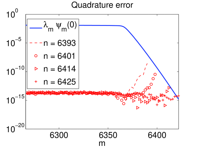
Figure 9: The quadrature error $\left|\int\psi_{m}-\sum\psi_{m}(t_{j})\cdot W_{j}\right|$ as a function of even $m<n$, for four different values of $n$ and $c=10000$. See Experiment 12.

In Figure 9, we display the results of the same experiment with different choice of parameters $c$ and $n$. Namely, we choose $c=10000$ and plot $\lambda_{m}\psi_{m}(0)$ as a function of even $0\leq m<6425$, on the logarithmic scale (solid blue line). In addition, we plot the absolute value of the quadrature error (654), as a function of $m$, for four different values of $n$: $n=6393$ (red dashed line), $n=6401$ (red circles), $n=6414$ (red triangles), and $n=6425$ (red pluses). The corresponding values of $|\lambda_{n}|$ are displayed in Table 17.

$n$	6393	6401	6414	6425
$|\lambda_{n}|$	0.43299E-07	0.54119E-09	0.33602E-12	0.52616E-15

Table 17: Values of $|\lambda_{n}|$ for $c=10000$ and different choices of $n$.

We make the following observations from Figure 9. First, $\lambda_{m}\psi_{m}(0)$ is approximately a constant for $m<2c/\pi$, and decays roughly exponentially with $m$ for $m>2c/\pi$. Also, for each value of $n$, the quadrature error (654) is essentially zero for $m<2c/\pi$, and its absolute value increases roughly exponentially with $m$ for $m>2c/\pi$. Nevertheless, the absolute error of the quadrature error is always bounded from above by $|\lambda_{n}|$, for each $n$. See also Tables 16, 18 and Conjecture 2 below.

$c$	$n$	$m$	$\lambda_{m}\psi_{m}(0)$	$\int\psi_{m}-\sum W_{j}\psi_{m}(t_{j})$	$\left|\lambda_{n}\right|$
250	179	178	0.28699E-07	-.52496E-08	0.18854E-07
250	184	182	0.68573E-09	-.38341E-10	0.16130E-09
250	188	186	0.14108E-10	-.68758E-12	0.30500E-11
500	339	338	0.52368E-07	-.13473E-07	0.40938E-07
500	345	344	0.37412E-09	-.86136E-10	0.27418E-09
500	350	348	0.12148E-10	-.99816E-12	0.35537E-11
1000	659	658	0.42709E-07	-.14354E-07	0.38241E-07
1000	665	664	0.51665E-09	-.15924E-09	0.43991E-09
1000	671	670	0.52494E-11	-.15024E-11	0.42815E-11
2000	1297	1296	0.41418E-07	-.17547E-07	0.41740E-07
2000	1304	1302	0.77185E-09	-.15036E-09	0.37721E-09
2000	1311	1310	0.31078E-11	-.11386E-11	0.28754E-11
4000	2572	2570	0.54840E-07	-.15493E-07	0.33682E-07
4000	2579	2578	0.43032E-09	-.20771E-09	0.46141E-09
4000	2587	2586	0.28193E-11	-.12805E-11	0.29164E-11
8000	5119	5118	0.43268E-07	-.26751E-07	0.52899E-07
8000	5128	5126	0.50230E-09	-.16395E-09	0.33442E-09
8000	5136	5134	0.50508E-11	-.15448E-11	0.32132E-11
16000	10213	10212	0.42725E-07	-.30880E-07	0.56568E-07
16000	10222	10220	0.69663E-09	-.28201E-09	0.52821E-09
16000	10231	10230	0.34472E-11	-.22162E-11	0.42902E-11

Table 18: Relation between the quadrature error and $\left|\lambda_{n}\right|$. See Experiment 12.

We strengthen the observations above by repeating this experiment with several other values of band limit $c$ and prolate index $n$. The results are displayed in Table 18. This table has the following structure. The first and second column contain, respectively, the band limit $c$ and the prolate index $n$. The third column contains the even integer $0\leq m<n$ (the values of $m$ were chose to be close to $n$). The fourth column contains $\lambda_{m}\psi_{m}(0)$. The fifth column contains the quadrature error (654). The last column contains $|\lambda_{n}|$.

We make the following observations from Table 18. First, for each of the seven values of $c$, the three indices $n$ were chosen in such a way that $|\lambda_{n}|$ is between $10^{-12}$ and $10^{-7}$. The values of the band limit $c$ vary between $250$ (the first three rows) and $16000$ (the last three rows). For each $n$, the value of $m$ is chosen to be the largest even integer below $n$. This choice of $m$ yields the largest $\lambda_{m}\psi_{m}(0)$ and the largest quadrature error (654) among all $m<n$ (see also Table 16). Obviously, $|\lambda_{m}|$ and $|\lambda_{n}|$ are of the same order of magnitude, for this choice of $m$. We also observe that, for all the values of $c,n,m$, the absolute error of the quadrature error (654) is bounded from above by $|\lambda_{n}|$ (and is roughly equal to $|\lambda_{n}|/2$). In other words, the upper bound on the quadrature error, provided by Theorem 62 (see (657)), is somewhat overcautious.

We summarize these observations in the following conjecture.

Conjecture 2.

Suppose that $c>0$ is a positive real number, and $n>2c/\pi$ is an integer. Suppose also that $0\leq m<n$ is an integer. Suppose furthermore that $t_{1},\dots,t_{n}$ and $W_{1},\dots,W_{n}$ are, respectively, the nodes and weights of the quadrature, introduced in Definition 2 in Section 4.4. Then,

$$\left|\int_{-1}^{1}\psi_{m}(s)\;ds-\sum_{j=1}^{n}\psi_{m}(t_{j})W_{j}\right|\leq|\lambda_{n}|.$$ (658)

Remark 26.

Conjecture 2 provides a stronger inequality than that of Theorem 62. On the other hand, Conjecture 2 has been only supported by numerical evidence, while Theorem 62 has been rigorously proven.

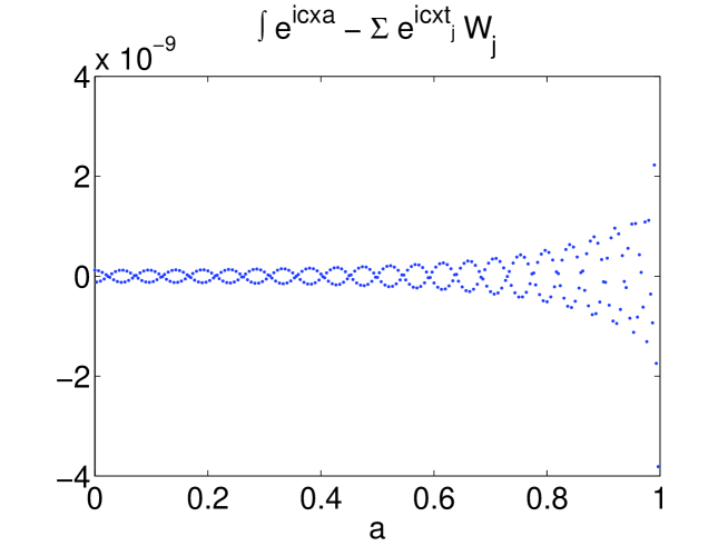
Figure 10: The quadrature error (661) with $c=1000$, $n=650$. See Experiment 13.

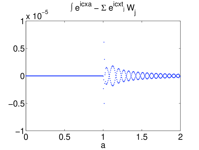
Figure 11: The quadrature error (661) with $c=1000$, $n=650$. See Experiment 13.

Experiment 13.

In this experiment, we demonstrate the performance of the quadrature, introduced in Definition 2 in Section 4.4, on exponential functions. We proceed as follows. We choose, more or less arbitrarily, the band limit $c$ and the prolate index $n$. We evaluate the quadrature nodes $t_{1},\dots,t_{n}$ and the quadrature weights $W_{1},\dots,W_{n}$, by using, respectively, the algorithms of Sections 5.3,  5.4 (in double precision). Also, we evaluate $|\lambda_{n}|$, by using the algorithm in Section 5.2 (in double precision). Then, we choose a real number $a\geq 0$, and evaluate the integral of $e^{icax}$ over $-1\leq x\leq 1$ via the formula

$$\int_{-1}^{1}e^{iacx}\;dx=\int_{-1}^{1}\cos(acx)\;dx=\frac{2\sin(ac)}{ac}.$$ (659)

Also, we compute an approximation to (659), by evaluating the sum

$$\sum_{j=1}^{n}W_{j}\cdot\cos(icat_{j}).$$ (660)

Finally, we evaluate the error of this approximation, that is,

$$\frac{2\sin(ac)}{ac}-\sum_{j=1}^{n}W_{j}\cdot\cos(icat_{j}).$$ (661)

In Figures 10, 11, we display the results of this experiment. The band limit and the prolate index were chosen to be, respectively, $c=1000$ and $n=650$. This choice yields $\lambda_{n}=$ -.21224E-04. In these figure, we plot the quadrature error (661) as a function of the real parameter $a$. Figure 10 corresponds to $0\leq a\leq 1$, while Figure 11 corresponds to $0\leq a\leq 2$.

We make the following observations from Figures 10, 11. For $0\leq a\leq 1$, the absolute value of the quadrature error (661) is bounded by $4\cdot 10^{-9}\approx 10\cdot|\lambda_{n}|^{2}$. The largest quadrature error is obtained when $a$ is close to 1. On the other hand, for $1\leq a\leq 2$, the absolute value of the quadrature error (661) is significantly larger, and is of order $|\lambda_{n}|$. The largest quadrature error is obtained when $a$ is close to 1.

These observations admit the following (somewhat imprecise) explanation. Suppose that $a\geq 0$ is a real number. Due to (37) and Theorem 1 in Section 2.1,

$$e^{iacx}=\sum_{m=0}^{\infty}\lambda_{m}\psi_{m}(a)\psi_{m}(x),$$ (662)

for all real $-1\leq x\leq 1$ (we note that while $e^{iacx}$ is not a bandlimited function of $-1\leq x\leq 1$, it does belong to $L^{2}\left[-1,1\right]$). Moreover,

$$\int_{-1}^{1}e^{iacx}\;dx=\frac{2\sin(ac)}{ac}=\sum_{m=0}^{\infty}\lambda_{m}^{2}\psi_{m}(a)\psi_{m}(0).$$ (663)

We combine (661), (662), (663), to obtain

$$\frac{2\sin(ac)}{ac}-\sum_{j=1}^{n}W_{j}\cdot\cos(icat_{j})=$$

$$\sum_{m=0}^{\infty}\lambda_{m}\psi_{m}(a)\left(\lambda_{m}\psi_{m}(0)-\sum_{j=1}^{n}W_{j}\psi_{m}(t_{j})\right).$$ (664)

We recall (see Experiment 12) that, for small values of $m$, the quadrature error (654) is very small compared to $|\lambda_{n}|$. On the other hand, for those values of $m<n$ that are close to $n$, the quadrature error (654) is of order $|\lambda_{n}|$. Therefore, roughly speaking,

$$\sum_{m=0}^{n-1}\lambda_{m}\psi_{m}(a)\left(\lambda_{m}\psi_{m}(0)-\sum_{j=1}^{n}W_{j}\psi_{m}(t_{j})\right)=O\left(|\lambda_{n}|^{2}\cdot\psi_{n-1}(a)\right).$$ (665)

On the other hand, due to the fast decay of $|\lambda_{m}|$, we expect

$$\sum_{m=n}^{\infty}\lambda_{m}\psi_{m}(a)\left(\lambda_{m}\psi_{m}(0)-\sum_{j=1}^{n}W_{j}\psi_{m}(t_{j})\right)=O\left(|\lambda_{n}|^{2}\cdot\psi_{n}(a)\right).$$ (666)

If $0\leq a\leq 1$, then $|\psi_{n}(a)|=O(\sqrt{n})$ (see Theorems 12, 13, 14 in Section 2.1). We combine this observation with (665), (666) to conclude that the quadrature error (661) is expected to be of the order $|\lambda_{n}|^{2}\cdot\sqrt{n}$.

If, on the other hand, $1\leq a\leq 2$, then $|\psi_{n}(a)|=O\left(|\lambda_{n}|^{-1}\right)$ (see, for example, Theorem 34 in Section 4.2.1, Theorem 43 in Section 4.2.2, Theorem 48 in Section 4.3.2, Experiment 1 in Section 6.1.1, Experiment 6 in Section 6.1.2). We combine this observation with (665), (666) to conclude that, in this case, the quadrature error (661) is expected to be of the order $|\lambda_{n}|$.

We summarize this crude analysis, supported by the observations above, in the following conjecture.

Conjecture 3.

Suppose that $c>0$ is a real number, and that $n>2c/\pi$ is an integer. Suppose also that $t_{1},\dots,t_{n}$ and $W_{1},\dots,W_{n}$ are, respectively, the nodes and weights of the quadrature, introduced in Definition 2 in Section 4.4. Suppose furthermore that $-1\leq a\leq 1$ is a real number. Then,

$$\int_{-1}^{1}e^{icax}\;dx-\sum_{j=1}^{n}e^{icat_{j}}\cdot W_{j}=O\left(|\lambda_{n}|^{2}\cdot\sqrt{n}\right).$$ (667)

Experiment 14.

In this experiment, we illustrate Theorems 64, 65 in Section 4.4.3. We proceed as follows. We choose, more or less arbitrarily, the band limit $c>0$ and the accuracy parameter $\varepsilon>0$. Then, we use the algorithm of Section 5.2 to find the minimal integer $m$ such that $|\lambda_{m}|<\varepsilon$. In other words, we define the integer $n_{1}(\varepsilon)$ via the formula

$$n_{1}(\varepsilon)=\min\left\{m\geq 0\;:\;|\lambda_{m}|<\varepsilon\right\}.$$ (668)

Also, we find the minimal integer such that the corresponding bound on the quadrature error, established in Theorem 62 in Section 4.4.2, is less that $\varepsilon$ (see also (657) in Experiment 12). In other words, we defined $n_{2}(\varepsilon)$ via the formula

$$n_{2}(\varepsilon)=\min\left\{m\geq 0\;:\;|\lambda_{m}|\cdot\left(24\cdot\log\left(\frac{1}{|\lambda_{m}|}\right)+6\cdot\chi_{m}\right)<\varepsilon\right\}.$$ (669)

Then, we define the integer $n_{3}(\varepsilon)$ via the formula (493) in Theorem 64. In other words,

$$n_{3}(\varepsilon)=\text{floor}\left(\frac{2c}{\pi}+\frac{\alpha(\varepsilon)}{2\pi}\cdot\log\left(\frac{16ec}{\alpha(\varepsilon)},\right)\right)$$ (670)

where $\alpha(\varepsilon)$ is defined via (492) in Theorem 64. Finally, we define the integer $n_{4}(\varepsilon)$ via the right-hand side of (506) in Theorem 65. In other words,

$$n_{4}(\varepsilon)=\text{floor}\left(\frac{2c}{\pi}+\left(10+\frac{3}{2}\cdot\log(c)+\frac{1}{2}\cdot\log\frac{1}{\varepsilon}\right)\cdot\log\left(\frac{c}{2}\right)\right).$$ (671)

In both (670) and (671), $\text{floor}(a)$ denotes the integer part of a real number $a$.

$c$	$\varepsilon$	$n_{1}(\varepsilon)$	$n_{2}(\varepsilon)$	$n_{3}(\varepsilon)$	$n_{4}(\varepsilon)$	$|\lambda_{n_{1}(\varepsilon)}|$	$|\lambda_{n_{2}(\varepsilon)}|$
250	$10^{-10}$	184	198	277	303	0.60576E-10	0.86791E-16
250	$10^{-25}$	216	227	326	386	0.31798E-25	0.14863E-30
250	$10^{-50}$	260	270	393	525	0.28910E-50	0.75155E-56
500	$10^{-10}$	346	362	460	488	0.49076E-10	0.60092E-16
500	$10^{-25}$	382	397	520	583	0.54529E-25	0.19622E-31
500	$10^{-50}$	433	446	607	742	0.82391E-50	0.38217E-56
1000	$10^{-10}$	666	687	803	834	0.95582E-10	0.92947E-17
1000	$10^{-25}$	707	725	875	942	0.97844E-25	0.14241E-31
1000	$10^{-50}$	767	783	981	1120	0.39772E-50	0.56698E-57
2000	$10^{-10}$	1305	1330	1467	1500	0.95177E-10	0.25349E-17
2000	$10^{-25}$	1351	1373	1550	1619	0.86694E-25	0.27321E-32
2000	$10^{-50}$	1418	1438	1675	1818	0.88841E-50	0.22795E-57
4000	$10^{-10}$	2581	2610	2768	2804	0.70386E-10	0.64396E-18
4000	$10^{-25}$	2632	2658	2862	2935	0.57213E-25	0.53827E-33
4000	$10^{-50}$	2707	2730	3007	3154	0.56712E-50	0.88819E-58
8000	$10^{-10}$	5130	5163	5344	5383	0.59447E-10	0.22821E-18
8000	$10^{-25}$	5185	5216	5450	5526	0.87242E-25	0.16237E-33
8000	$10^{-50}$	5268	5296	5614	5765	0.95784E-50	0.23927E-58
16000	$10^{-10}$	10225	10264	10468	10509	0.63183E-10	0.37516E-19
16000	$10^{-25}$	10285	10321	10585	10664	0.85910E-25	0.41416E-34
16000	$10^{-50}$	10377	10409	10769	10923	0.51912E-50	0.56250E-59
32000	$10^{-10}$	20413	20457	20686	20730	0.62113E-10	0.12818E-19
32000	$10^{-25}$	20478	20519	20815	20897	0.78699E-25	0.12197E-34
32000	$10^{-50}$	20577	20615	21018	21176	0.96802E-50	0.15816E-59
64000	$10^{-10}$	40786	40837	41092	41139	0.89344E-10	0.28169E-20
64000	$10^{-25}$	40857	40903	41232	41318	0.66605E-25	0.39212E-35
64000	$10^{-50}$	40964	41008	41454	41616	0.85451E-50	0.28036E-60

Table 19: Illustration of Theorems 64, 65. See Experiment 14.

We display the results of this experiment in Table 19. This table has the following structure. The first column contains the band limit $c$. The second column contains the accuracy parameter $\varepsilon$. The third column contains $n_{1}(\varepsilon)$, defined via (668). The fourth column contains $n_{2}(\varepsilon)$, defined via (669). The fifth column contains $n_{3}(\varepsilon)$, defined via (670). The sixth column contains $n_{4}(\varepsilon)$, defined via (671). The seventh column contains $|\lambda_{n_{1}(\varepsilon)}|$. The last column contains $|\lambda_{n_{2}(\varepsilon)}|$.

Suppose that $c>0$ is a band limit, and $n>0$ is an integer. We define the real number $Q(c,n)$ via the formula

$$Q(c,n)=\max\left\{\left|\int_{-1}^{1}\psi_{m}(t)\;dt-\sum_{j=1}^{n}\psi_{m}(t_{j})\cdot W_{j}\right|\;:\;0\leq m\leq n-1\right\},$$ (672)

where $t_{1},\dots,t_{n}$ and $W_{1},\dots,W_{n}$ are, respectively, the nodes and the weights of the quadrature, defined in Definition 2 in Section 4.4. In other words, this quadrature rule integrates the first $n$ PSWFs up to an error at most $Q(c,n)$.

We make the following observations from Table 19. We observe that $Q(c,n_{1}(\varepsilon))<\varepsilon$, due to the combination of Conjecture 2 in Section 6.2.1 and (668), (672). In other words, numerical evidence suggests that the quadrature of order $n_{1}(\varepsilon)$ will integrate the first $n_{1}(\varepsilon)$ PSWFs up to an error at most $\varepsilon$ (see Remark 26). On the other hand, we combine Theorem 62 in Section 4.4.2 with (669), (672), to conclude that the quadrature of order $n_{2}(\varepsilon)$ has been rigorously proven to integrate the first $n_{2}(\varepsilon)$ PSWFs up to an error at most $\varepsilon$. In both Theorem 62 and Conjecture 2, we establish upper bounds on $Q(c,n)$ in terms of $|\lambda_{n}|$. The ratio of $|\lambda_{n_{1}(\varepsilon)}|$ to $|\lambda_{n_{2}(\varepsilon)}|$ is quite large: from about $10^{6}$ for $c=250$ and $\varepsilon=10^{-10},10^{-25},10^{-50}$ (see the first three rows in Table 19), to about $10^{10}$ for $c=64000$ and and $\varepsilon=10^{-10},10^{-25},10^{-50}$ (see the last three rows in Table 19). On the other hand, the difference between $n_{2}(\varepsilon)$ and $n_{1}(\varepsilon)$ is fairly small; for example, for $\varepsilon=10^{-50}$, this difference varies from 10 for $c=250$ to $23$ for $c=4000$, to merely $44$ for as large $c$ as $c=64000$.

As opposed to $n_{1}(\varepsilon)$ and $n_{2}(\varepsilon)$, the integer $n_{3}(\varepsilon)$, defined via (670), is computed via an explicit formula that depends only on $c$ and $\varepsilon$ (rather than on $|\lambda_{n}|$ and $\chi_{n}$, that need to be evaluated numerically). This formula is derived in Theorem 64 by combining Theorem 62 with some explicit bounds on $|\lambda_{n}|$ and $\chi_{n}$ in terms of $c$ and $n$. The convenience of (670) vs. (668), (669) comes at a price: for example, for $\varepsilon=10^{-50}$, the difference between $n_{3}(\varepsilon)$ and $n_{2}(\varepsilon)$ is 123 for $c=250$, and 446 for $c=64000$. However, the difference $n_{3}(\varepsilon)-n_{2}(\varepsilon)$ is rather small compared to $c$: for example, for $\varepsilon=10^{-50}$, this difference is roughly $4\cdot\left(\log(c)\right)^{2}$, for all the values of $c$ in Table 19.

Furthermore, we observe that $n_{4}(\varepsilon)$ is also computed via an explicit formula that depends only on $c$ and $\varepsilon$ (see (671)). This formula is a simplification of that for $n_{3}(\varepsilon)$, derived in Theorem 65. Thus, not surprisingly, $n_{4}(\varepsilon)$ is greater than $n_{3}(\varepsilon)$, for all the values of $c$ and $\varepsilon$.

We summarize these observations as follows. Suppose that the band limit $c$ and the accuracy parameter $\varepsilon>0$ are given. In Theorem 64, we prove that $n\geq n_{3}(\varepsilon)$ implies that the quadrature error $Q(c,n)$, defined via (672), will be at most $\varepsilon$ (for the quadrature of order $n$, defined in Definition 2 in Section 4.4). On the other hand, numerical evidence suggests that $Q(n,c)<\varepsilon$ also for all the values of $n$ between $n_{1}(\varepsilon)$ and $n_{3}(\varepsilon)$ (see Experiment 12). In this experiment, we observed that the difference between $n_{3}(\varepsilon)$ and $n_{1}(\varepsilon)$ is relatively small compared to $c$ (roughly of order $\left(\log(c)\right)^{2}$).

6.2.2 Quadrature Weights

Experiment 15.

In this experiment, we illustrate the results of Section 4.4.4 (in particular, Theorem 67, Corollary 5 and Remark 14). We proceed as follows. We choose, more or less arbitrarily, band limit $c$ and prolate index $n$. Then, we compute the quadrature nodes $t_{1},\dots,t_{n}$ as well as $\psi_{n}^{\prime}(t_{1}),\dots,\psi_{n}^{\prime}(t_{n})$, by using the algorithm of Section 5.3. We evaluate $\psi_{n}^{\prime}(0)$, using the algorithm of Section 5.1. Next, we evaluate the quadrature weights $W_{1},\dots,W_{n}$, by using the algorithm of Section 5.4. Also, for each $j=1,\dots,n$, we evaluate the sum

$$-\frac{2}{\psi_{n}^{\prime}(t_{j})}\sum_{k=0}^{\infty}\alpha_{k}^{(n)}Q_{k}(t_{j}),$$ (673)

where $Q_{k}(t)$ is the $k$th Legendre function of the second kind, defined in Section 2.2, and $\alpha_{k}^{(n)}$ is the $k$th coefficient of the Legendre expansion of $\psi_{n}$, defined via (84) in Section 2.2 (see Theorem 67 and Section 5.1). To evaluate (673) numerically, we use only $2N$ first summands, where $N$ is an integer of order $n$ (see (587) in Section 5.1). All the calculations are carried out in double precision.

$j$	$W_{j}$	$W_{j}+2\cdot\tilde{\Phi}_{n}(t_{j})/\psi_{n}^{\prime}(t_{j})$	$W_{j}-\frac{W_{21}\left(\psi_{n}^{\prime}(0)\right)^{2}}{\left(\psi_{n}^{\prime}(t_{j})\right)^{2}\cdot\left(1-t_{j}^{2}\right)}$
1	0.7602931556894E-02	0.00000E+00	-.55796E-11
2	0.1716167229714E-01	0.00000E+00	-.55504E-10
3	0.2563684665002E-01	0.00000E+00	-.21825E-12
4	0.3278512460580E-01	0.00000E+00	-.11959E-09
5	0.3863462966166E-01	0.16653E-15	0.82238E-11
6	0.4334940472363E-01	0.22204E-15	-.16247E-09
7	0.4713107235981E-01	0.22204E-15	0.11270E-10
8	0.5016785516291E-01	0.19429E-15	-.18720E-09
9	0.5261660773966E-01	0.26368E-15	0.10495E-10
10	0.5460119701692E-01	0.29837E-15	-.20097E-09
11	0.5621699326080E-01	0.17347E-15	0.81464E-11
12	0.5753664411864E-01	0.12490E-15	-.20866E-09
13	0.5861531690539E-01	0.10408E-15	0.55098E-11
14	0.5949490764741E-01	0.23592E-15	-.21301E-09
15	0.6020725336886E-01	0.13184E-15	0.31869E-11
16	0.6077650804037E-01	0.18041E-15	-.21545E-09
17	0.6122088420703E-01	0.48572E-16	0.14361E-11
18	0.6155390478472E-01	0.83267E-16	-.21675E-09
19	0.6178529976346E-01	0.11102E-15	0.36146E-12
20	0.6192162112196E-01	0.48572E-16	-.21732E-09
21	0.6196665001384E-01	0.00000E+00	0.00000E+00

Table 20: Quadrature weights (434) with $c=40$, $n=41$. $\lambda_{n}=\mbox{\text{\rm{i0.69857E-08}}}$. See Experiment 15.

We display the results of this experiment Table 20. The data in this table correspond to $c=40$ and $n=41$. Table 20 has the following structure. The first column contains the weight index $j$, that varies between 1 and $21=(n+1)/2$. The second column contains $W_{j}$. The third column contains the difference between $W_{j}$ and (673). The last column contains the difference

$$W_{j}-\frac{W_{21}\left(\psi_{n}^{\prime}(0)\right)^{2}}{\left(\psi_{n}^{\prime}(t_{j})\right)^{2}\cdot\left(1-t_{j}^{2}\right)}$$ (674)

(see Remark 14).

In Figure 12, we plot the weights $W_{j}$, displayed in the second column of Table 20. For $j>21$, the weights are computed via symmetry considerations. Each $W_{j}$ is plotted as a red dot above the corresponding node $t_{j}$.

We make the following observations from Table 20. First, all the weights are positive (see Theorem 73 and Remark 13). Moreover, $W_{j}$ grow monotonically as $j$ increases to $(n+1)/2$. Also, due to the combination of Theorems 67, 68 in Section 4.4.4, the value in the third column would be zero in exact arithmetics. We observe that, indeed, this value is zero up to the machine precision, which confirms the correctness of the algorithm of Section 5.4. (We note that, for $j=1,2,3,4$ and $j=21$, this algorithm, in fact, does evaluate $W_{j}$ via (673), and hence this value in the corresponding rows is exactly zero). Finally, we observe that, for all $j$, the value (674) in the last column is of the order $|\lambda_{n}|$, in correspondence with Remark 14.

Figure 12: The quadrature weights $W_{1},\dots,W_{n}$ with $c=40$, $n=41$. See Experiment 15.

References

- [1] M. Abramowitz, I. A. Stegun, Handbook of Mathematical Functions with Formulas, Graphs and Mathematical Tables, Dover Publications, 1964.
- [2] W. Barth, R. S. Martin, J. H. Wilkinson, Calculation of the Eigenvalues of a Symmetric Tridiagonal Matrix by the Method of Bisection, Numerische Mathematik 9, 386-393, 1967.
- [3] Carl Bender, Steven Orszag, Advanced Mathematical Methods for Scientists and Engineers, McGraw-Hil, Inc. 1978.
- [4] C. J. Bouwkamp, On spheroidal wave functions of order zero, J. Math. Phys. 26, 79-92, 1947.
- [5] W. E. Boyce, R. C. DiPrima, Elementary Differential Equations and Boundary Value Problems, Seventh Edition, John Wiley and Sons, Inc., 2001.
- [6] H. Cheng, N. Yarvin, V. Rokhlin, Non-linear Optimiuzation, Quadrature and Interpolation, SIAM J. Optim. 9, 901-23, 1999.
- [7] G. Dahlquist, A. Björk, Numerical Methods, Prentice-Hall Inc., 1974.
- [8] L.C. Evans, Partial Differential Equations, Graduate Studies in Mathematics Vol. 19, AMS (1998).
- [9] M.V. Fedoryuk, Asymptotic Analysis of Linear Ordinary Differential Equations, Springer-Verlag, Berlin (1993).
- [10] C. Flammer, Spheroidal Wave Functions, Stanford, CA: Stanford University Press, 1956.
- [11] Andreas Glaser, Xiangtao Liu, Vladimir Rokhlin, A fast algorithm for the calculation of the roots of special functions, SIAM J. Sci. Comput., 29(4):1420-1438 (electronic), 2007.
- [12] I.S. Gradshteyn, I.M. Ryzhik, Table of Integrals, Series, and Products, Seventh Edition, Elsevier Inc., 2007.
- [13] D. B. Hodge, Eigenvalues and Eigenfunctions of the Spheroidal Wave Equation, J. Math. Phys. 11, 2308-2312, 1970.
- [14] E. Isaacson, H. B. Keller, Analysis of Numerical Methods, New York: Wiley, 1966.
- [15] S. Karlin, W. J. Studden, Tchebycheff Systems with Applications in Analysis and Statistics, Wiley-Interscience, New York, 1966.
- [16] M. G. Krein, The Ideas of P. L. Chevyshev and A. A. Markov in the THeory of Limiting Values of Integrals, AM. Math. Soc. Trans., 12, 1-122, 1959.
- [17] H. J. Landau, H. O. Pollak, Prolate spheroidal wave functions, Fourier analysis, and uncertainty - II, Bell Syst. Tech. J. January 65-94, 1961.
- [18] H. J. Landau, H. Widom, Eigenvalue distribution of time and frequency limiting, J. Math. Anal. Appl. 77, 469-81, 1980.
- [19] Daniel C. Lewis, Inequalities for complex linear differential systems of the second order, Proc Natl Acad Sci U S A, 1952 January, 38(1): 63–66.
- [20] J. Ma, V. Rokhlin, S. Wandzura, Generalized Gaussian Quadratures for Systems of Arbitrary Functions, SIAM J. Numer. Anal. 33, 971-96, 1996.
- [21] A. A. Markov, On the Limiting Values of Integrals in Connection with Interpolation, Zap. Imp. Akad. Nauk. Fiz.-Mat. Otd. (8) 6, no 5 (in Russian), 1898.
- [22] A. A. Markov, Selected Papers on Continued Fractions and the Theory of Functions Deviating Least From Zero, OGIZ: Moscow (in Russian), 1948.
- [23] Richard K. Miller, Anthony N. Michel, Ordinary Differential Equations, Dover Publications, Inc., 1982.
- [24] P. M. Morse, H. Feshbach, Methods of Theoretical Physics, New York McGraw-Hill, 1953.
- [25] A. Osipov, Non-asymptotic Analysis of Bandlimited Functions, Yale CS Technical Report #1449, 2012.
- [26] A. Osipov, Certain inequalities involving prolate spheroidal wave functions and associated quantities, arXiv:1206.4056v1, 2012.
- [27] A. Osipov, Explicit upper bounds on the eigenvalues associated with prolate spheroidal wave functions, Yale CS Technical Report #1450, 2012.
- [28] A. Osipov, Certain upper bounds on the eigenvalues associated with prolate spheroidal wave functions, arXiv:1206.4541v1, 2012.
- [29] A. Papoulis, Signal Analysis, Mc-Graw Hill, Inc., 1977.
- [30] Vladimir Rokhlin, Hong Xiao, Approximate Formulae for Certain Prolate Spheroidal Wave Functions Valid for Large Value of Both Order and Band Limit.
- [31] W. Rudin, Real and Complex Analysis, Mc-Graw Hill Inc., 1970.
- [32] Yoel Shkolnisky, Mark Tygert, Vladimir Rokhlin, Approximation of Bandlimited Functions.
- [33] D. Slepian, Some comments on Fourier analysis, uncertainty, and modeling, SIAM Rev.(3) 379-93, 1983.
- [34] D. Slepian, H. O. Pollak, Prolate spheroidal wave functions, Fourier analysis, and uncertainty - I, Bell Syst. Tech. J. January 43-63, 1961.
- [35] D. Slepian, H. O. Pollak, Prolate spheroidal wave functions, Fourier analysis, and uncertainty - IV: extensions to many dimensions, generalized prolate spheroidal wave functions, Bell Syst. Tech. J. November 3009-57, 1964.
- [36] D. Slepian, Some asymptotic expansions for prolate spheroidal wave functions, J. Math. Phys. 44 99-140, 1965.
- [37] J. H. Wilkinson, Algebraic Eigenvalue Problem, Oxford University Press, New York, 1965.
- [38] H. Xiao, V. Rokhlin, N. Yarvin, Prolate spheroidal wavefunctions, quadrature and interpolation, Inverse Problems, 17(4):805-828, 2001.
- [39] N. Yarvin, V. Rokhlin, Generalized Gaussian Quadratures and Singular Value Decompositions of Integral Operators, SIAM J. Sci. Comput. 20, 699-718, 1998.