Identifying dynamical systems with bifurcations from noisy partial observation

Abstract

Dynamical systems are used to model a variety of phenomena in which the bifurcation structure is a fundamental characteristic. Here we propose a statistical machine-learning approach to derive low-dimensional models that automatically integrate information in noisy time-series data from partial observations. The method is tested using artificial data generated from two cell-cycle control system models that exhibit different bifurcations, and the learned systems are shown to robustly inherit the bifurcation structure.

Various phenomena ranging from climate change to chemical reactions have been modeled extensively by dynamical systems Saltzman (2001); Strogatz (2001), and the relevance of dynamical systems to modeling biological phenomena is being increasingly recognized Kaneko (2006); Alon (2006). Recent advances in experimental techniques such as live-cell imaging that clarifies molecular activities at high spatiotemporal resolutions Stephens and Allan (2003); Shav-Tal et al. (2004); Fernández-Suárez and Ting (2008) have accompanied this recognition. However, noise, partial observation, and a low controllability are still challenges for measuring biological systems in that both the system dynamics and measurement processes are highly stochastic, only a few components in a system are observable, and only a small number of experimental conditions can be examined. These difficulties have led to models being constructed from experimental observations in a way that is often ad-hoc and semi-quantitative at best because instructive criteria and practical methods have not yet been established for deriving the model equations by systematically integrating the information in the experimental data.

To model complex systems such as cellular processes, a full description of all the systems details is often impractical and not informative. Instead, a reduced description that preserves the essential features of the system is more useful for comprehension., i.e., models described by low-dimensional dynamical systems are sufficient for explaining experimental observations. In particular, the bifurcation structure is a fundamental feature of dynamical systems since it characterizes the qualitative changes of the dynamics. Thus, identification of low-dimensional model systems that inherit the original bifurcation structure is a crucial step in understanding the dynamics.

Here we propose a statistical machine-learning approach to automatically derive the low-dimensional model equations from single-cell time-series data obtained at a few conditions (i.e., bifurcation parameter values; Fig. 1). Techniques for learning nonlinear dynamical systems from time-series data have been employed for chaos Judd and Mees (1996); Wang et al. (2011), spatiotemporal patterns Voss et al. (1999); Müller and Timmer (2002); Sitz et al. (2003), and multi-stable systems Ohkubo (2011). Only a few studies have applied the technique to biological data Nagasaki et al. (2006); Yoshida et al. (2008). In a similar manner to some of those studies Nagasaki et al. (2006); Yoshida et al. (2008), we employ a statistical technique to deal with the noisy and partial time-series data. However, rather than aiming to fit the model parameters to the observation, we obtain the low-dimensional model equations that inherit bifurcation structure of the full system to capture the basic nature of the observed system. The performance of the method is demonstrated by using artificial data.

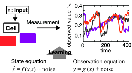
Figure 1: Schematic representation of the proposed method. Time-series data of the molecular activities in individual cells are obtained from measurements under a given input level $s$, which is regarded as a bifurcation parameter of the system. System and observation equations are then trained to reproduce the time-series data.

We introduce a nonlinear state space model composed of state and observation equations that describe the system dynamics and observation process, respectively. We consider a system that is modeled by a $D$-dimensional stochastic differential equations, and $d$ components in the model can be simultaneously observed. The state equations are discretized in time by the Euler-Maruyama scheme Kloeden and Platen (1999). We write the time evolution of the $i$th variable at a time point $t$, $x_{i}^{t}(i=1,\dots,D)$, as

$$x_{i}^{t+1} = x_{i}^{t}+\Delta tf_{i}(\{x_{j}^{t}\},s)+\sigma_{i}\xi_{i}^{t}\sqrt{\Delta t},$$ (1)

where $\Delta t$ is an integration time, $\sigma_{i}$ is the intensity of the system noise, and $s$ is a bifurcation parameter. System noise $\xi_{i}^{t}$ is sampled from a standard normal distribution. To achieve efficient learning, the function $f_{i}$ is considered to be expressed by a summation of linearly independent functions as $f_{i}(\{x_{j}^{t}\},s)=\sum_{n}^{N_{i}}k_{i}^{n}f_{i}^{n}(\{x_{j}\},s)$, where $N_{i}$ is the number of parameters $\{k_{i}^{n}\}$ and functions $\{f_{i}^{n}\}$. Since our aim is to reproduce the bifurcation structures of systems subjected to unknown equations, we adopt a polynomial base for the $\{f_{i}^{n}\}$, rather than biochemically realistic functions like the Michaelis-Menten equation.

The observation value of the $i$ th component at a time point $r$, $y_{i}^{r}(i=1,\dots,d)$, is written as

$$y_{i}^{r} = g_{i}(x_{i}^{r})+\eta_{i}\phi_{i}^{r}$$ (2)

where $\eta_{i}$ is an observation noise intensity, and $\phi_{i}^{r}$ is sampled from a standard normal distribution. In general, a set of observed time points is a part of the entire set of time points in the numerical integration. Hereafter, $\theta$ indicates the parameters to be estimated: $\left(\{k_{i}^{n}\},\{\sigma_{i}\},\{\eta_{i}\}\right)$.

The learning of dynamical systems is formulated as a maximum likelihood (ML) estimation, which is summarized below (further details are given in the section 1 in the Supplemental Material). The likelihood is given by the conditional probability of the observed time series $Y$ as a function of the model parameters $\theta$. However, a straightforward maximization of the likelihood $p(Y|\theta)$ is difficult because it requires the untractable summation of $p(Y|X,\theta)p(X|\theta)$ with respect to the time series of the state variables $X$. Thus, we employ the EM algorithm to maximize the log likelihood of a model by a two-step iterative method that alternately estimates the states and parameters Dempster et al. (1977). In the first step, the E step, the posterior distribution of the time series of a state ($p(X|Y,\theta)$) is estimated based on the tentative parameter set $\theta_{\rm old}$. In the second step, the M step, the expectation value of $\log p(X,Y|\theta)$ is calculated as

$$Q(\theta,\theta_{\rm old})=\langle\log p(X,Y|\theta)\rangle_{p(X|Y,\theta_{\rm old})},$$ (3)

and the parameter estimation is updated as

$$\theta_{\rm new}=\operatornamewithlimits{argmax}_{\theta}Q(\theta,\theta_{\rm old}).$$ (4)

In this step, the optimization problem is reduced to linear simultaneous equations and thus can be solved easily. However, the problem in the E step is still analytically unsolvable because the probability distribution of the time series is necessary. This calculation requires a state estimation at all time points including the points at which measurements are not conducted. We therefore obtain a numerical approximation of $p(X|Y,\theta)$ using a particle filter algorithm that performs state estimations of nonlinear models using a Monte-Carlo method Gordon et al. (1993); Kitagawa (1996). The particle filter (a numerical extension of Kalman filter) approximates a general non-Gaussian state distribution as a set of particles representing samples from the distribution and evaluates the log likelihood of the models. Since the use of the particle filter introduces stochasticity into the learning algorithm, a slight modification of the M step is required to ensure convergence of the learning Delyon et al. (1999). The optimization function in eq.(4) is replaced by $Q^{\prime}_{I}(\theta)=(1-\alpha_{I})Q^{\prime}_{I-1}(\theta)+\alpha_{I}Q(\theta,\theta_{\rm old})$, where $I$ is the iteration index, and $\{\alpha_{I}\}$ is a sequence of non-increasing positive numbers converging to zero.

To validate the method, we apply it to artificial data generated from models of a eukaryotic cell cycle control system since this system provides an illustrative example of cellular dynamics composed of many molecular components Novak and Tyson (1993a); Borisuk and Tyson (1998); Pomerening et al. (2005); Tsai et al. (2008); Pfeuty et al. (2008). The cell cycle is a fundamental biological process characterized by repeated events underlying cell division and growth in which key proteins, Cyclin and Cyclin-dependent kinases, change their concentration periodically and activate various cellular functions such as DNA synthesis.

Two molecular circuit models of the cell-cycle control system in Xenopus embryos are adopted as the data generators: that proposed by Tyson and co-workers (the Tyson model) Novak and Tyson (1993a); Borisuk and Tyson (1998), and that proposed by Ferrell and co-workers (the Ferrell model) Pomerening et al. (2005); Tsai et al. (2008). Although both models show an oscillation onset as the synthesis rate of Cyclin increases, they differ in the type of bifurcation at the onset; the Tyson model exhibits a saddle-node bifurcation on an invariant circle (SNIC), while the Ferrell model exhibits a supercritical Hopf bifurcation. We investigate whether the proposed learning procedure reproduces the correct bifurcation types of each model.

Both data generators are composed of 9 variables including Cdc2, Cyclin, and other regulatory proteins. The time-series data is generated by a numerical calculation of these models as nonlinear Langevin equations at a few parameter values (see the section 2 in the Supplemental Material for the model equations, and obtained time-series data). We simulate noisy observation by adding Gaussian noise to each observation value. Artificial data are prepared for three Cyclin synthesis rates across the bifurcation point, and for each bifurcation parameter value, three independent time series are prepared in which the oscillation exhibits a large fluctuation in amplitude and period among the samples.

Considering a polynomial of degree $M$, we write the system equations to be learned as

$$f_{i}(\{x_{j}^{t}\},s)=k_{i}^{1}+k_{i}^{2}x_{1}^{t}+k_{i}^{3}x_{2}^{t}+\dots+k_{i}^{N_{i}}(x_{D}^{t})^{M}$$ (5)

The observation equations are expressed simply as $y_{i}^{r}=x_{i}^{r}+\eta_{i}\phi_{i}^{r}$. We consider the active Cdc2 and Cyclin concentrations to be observable variables since their levels have been observed in previous experiments Pomerening et al. (2005). Accordingly, $y_{1}$ $(x_{1})$ and $y_{2}$ $(x_{2})$ represent the observed (true) concentrations of active Cdc2 and Cyclin, respectively. The other variables $x_{i}$ $(i>2)$ represent the true concentrations of unobservable components. In the system, the Cyclin synthesis rate, $s$, is a bifurcation parameter. We take the constant term in the equation for Cyclin to be the synthesis rate, i.e., $k_{2}^{1}=s$. Note that the observed orbit in the active Cdc2-Cyclin plane exhibits no intersection, (see Fig. S1 in the Supplemental Material) suggesting that the two variables are sufficient to abstract the original high-dimensional dynamics.

The simplest polynomial form required for reproducing the observed dynamics is determined by starting with linear equations composed of active Cdc2 and Cyclin (system dimension $D=2$ and polynomial order $M=1$) and increasing the $D$ and $M$ by one. It turns out that $D=2$ is sufficient for reproducing a given time-series data set as shown below. The polynomial order $M$ is determined by minimizing the information criteria through an optimization of the balance between the goodness of fit and the model complexity Akaike (1974); Schwarz (1978). The Akaike information criterion (AIC) and Bayesian information criterion (BIC) are evaluated from the log likelihood, parameter number, and data size for each model (Fig.2). Both the AIC and BIC show a decrease from $M=1$ to $3$, but an increase or insignificant decrease at $M=4$. Therefore, we analyze models with $D=2$ and $M=3$ (see the section 3 in the Supplemental Material for the learned parameter values and detailed settings in the learning algorithm).

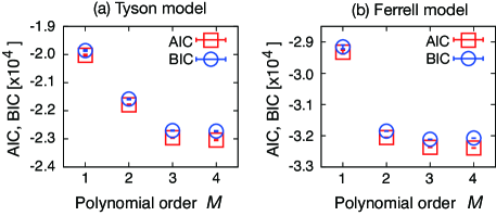
Figure 2: The AIC and BIC are plotted against different polynomial orders $M=1,2,3,4$ for the (a) Tyson and (b) Ferrell models. For each evaluation, 20 different initial parameters are sampled to avoid the local minima. After the learning, the average and standard deviation are calculated from 100 evaluation trials based on the particle filter.

To check whether the learning procedure can capture the bifurcation of the original data generator system, we compare the bifurcation diagrams of the learned systems with those of the data generators. Figures 3(a) and (b) show bifurcation diagrams against Cyclin synthesis rate $s$ (red lines) for the learned systems in the Tyson and Ferrell models, respectively. The bifurcation diagrams for the corresponding noiseless data generators are shown by the gray lines. Although the data for the learning are given only at three bifurcation parameter points (indicated by the broken lines), the learned systems have quantitatively similar diagrams to those of the corresponding data generators. The sudden appearance of a limit cycle with finite amplitude is reproduced for the Tyson model, while the gradual increase in amplitude from the bifurcation point is reproduced for the Ferrell model. These features are characteristics of the SNIC and supercritical Hopf bifurcation. Nullclines of the learned systems in the vicinity of the bifurcation points are shown in Figs. 3(c) and (d) for the Tyson model and in Figs. 3(e) and (f) for the Ferrell model. The results confirm the onset of SNIC and supercritical Hopf bifurcation, respectively. Thus, each learned system inherits the bifurcation type of the original model through the learning procedure in spite of noisy and partial observations.

When the learning is conducted by using the data on two of the three bifurcation parameter points, the learned systems still exhibit the correct bifurcation types, although the points of oscillation onset and amplitudes are biased (Figs. 3(g) and (h)). Note that identification of bifurcation is possible even by using the data only on one side of a bifurcation point (as indicated by the green lines). These results indicate the interesting possibility that the learning procedure can predict the type of bifurcation that will occur from the data before the bifurcation point only.

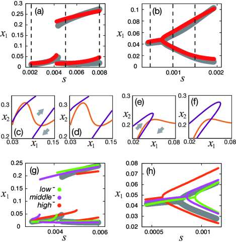
Figure 3: Bifurcation diagrams of the (a) Tyson and (b) Ferrell models. The active Cdc2 concentration $x_{1}$ for the learned systems is plotted against the Cyclin synthesis rate $s$ (red), and corresponding concentrations of the data generators are also shown for comparison (gray). The broken lines indicate points at which the data are given. For the Tyson model, there is another attractor with a tiny basin that is ignored. (c-f) The nullclines of the learned systems around the bifurcation points are shown. Purple and orange lines represent nullclines of $x_{1}$ (active Cdc2) and $x_{2}$ (Cyclin), respectively, and the gray arrows indicate the flow direction. (c,d) The learned system from the Tyson model exhibits SNIC and (e,f) that from the Ferrell model exhibits a supercritical Hopf bifurcation. The values of the bifurcation parameter are (c) $s=0.0038$, (d) $0.0044$, (e) $0.0005$, and (f) $0.0012$, respectively. (g,h) Bifurcation diagrams using the data at two of the three bifurcation parameter points. The learning that lacks data at the lowest, intermediate, and highest bifurcation parameter values are denoted by as $low^{-}$, $middle^{-}$ and $high^{-}$, respectively.

We also show here how the high-dimensional phase space structures of the original data generators are mapped onto the lower-dimensional surfaces in the learned systems. Reduced two-variable models are derived by adiabatic elimination following a similar procedure by Novak and Tyson Novak and Tyson (1993b) (see the section 4 in the Supplemental Material for the detailed procedure and reduced model equations). Like the learned systems, the reduced models are composed of active Cdc2 and total Cyclin. Figure 4 shows the nullclines of the learned systems (the solid orange and purple lines) and the reduced models (the broken lines). In both the Tyson and Ferrell models, the learned system and reduced model nullclines for active Cdc2 have a similar $N$-shaped form (orange lines), indicating the existence of positive feedback in the molecular circuits. In contrast, those for the total Cyclin disagree quite significantly. To check the consistency of the nullclines and dynamics, Fig. 4 also shows a noisy time series from the data generators (blue points) and the orbit of the learned system (red lines). The nullclines of the learned systems are consistent with the dynamics in the data but the reduced models are not. This failure arises because the dynamics of a component mediating the inhibition from active Cdc2 to Cyclin is not fast enough to allow the adiabatic approximation. Higher-order contribution beyond the adiabatic elimination performed here should be included, which requires complicated technical work. Nevertheless, the learning process automatically reproduces the appropriate low-dimensional dynamics and estimates the bifurcation structures without knowledge of the detailed high-dimensional model systems.

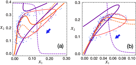
Figure 4: Comparison of the learned systems and reduced models for the (a) Tyson and (b) Ferrell models. The purple and orange lines represent the nullclines of $x_{1}$ (active Cdc2) and $x_{2}$ (Cyclin), respectively, for the learned systems (solid lines) and reduced models (broken lines). A noisy time series from the data generators (blue dots) and the orbits of the learned models (red lines) are also shown. The blue arrows indicate the flow direction. The values of the bifurcation parameter are (a) $s=0.006$, (b) $0.0015$.

Gathering biological data is complicated by intrinsic and observation noises, partial observation, and a small number of possible experimental conditions. We have outlined here a machine-learning procedure based on likelihood maximization that makes use of all the information in the time-series data, including that in the noise. By using synthetic data that share the difficulties found in actual biological data, we demonstrated that the procedure could derive low-dimensional model equations that reproduced the obtained time-series data and captured the bifurcation types of the original systems. These results support the conjecture that the learning procedure will be able to construct reliable low-dimensional models for real time-series data of active Cdc2 and Cyclin levels in future studies. Being able to identify the model systems and bifurcation types will provide a useful method for elucidating both the molecular interactions in the circuit and the biological functions of the dynamics. Further, since the dynamics and bifurcation are found widely among various biological processes, the method is expected to be applicable to various cell system with cell-imaging data.

We note that the proposed procedure can be interpreted as a reduction method from high- to low-dimensional systems like adiabatic approximation. In particular, in the vicinity of the bifurcation points, the systems are usually reduced to normal forms represented by low-dimensional differential equations with low-order polynomial forms Guckenheimer and Holmes (1983). However, unlike analytical reduction methods that require the original high-dimensional equations, the present learning procedure uses only the time-series data. This is especially advantageous for studying cell dynamics that involve complex molecular interactions. On the other hand, since the learning method has a less theoretical basis for interpreting the obtained equations, it should be complemented by an analytical procedure.

In essence, the proposed method performs quantitative inference of the phase space structures of the dynamical systems. Therefore, not only the bifurcation structure but also other properties of the dynamical system can be analyzed using the same theoretical groundwork developed here. The detection of phase sensitivity from noisy data in studies of biological clocks Winfree (2001) would provide an interesting application. In addition, the method is flexible enough to be combined with other machine-learning techniques; it was recently shown that compressive sensing exhibits a high performance for learning dynamical systems Wang et al. (2011). Those possible extensions will further improve our method depending on the situations and experimental setup. In summary, the proposed method will be an efficient way to capture the essential features of the cellular dynamics by mediating dynamical system modeling with experimental observations.