Model of the Optical Emission of a Driven Semiconductor Quantum Dot: Phonon-Enhanced Coherent Scattering and Off-Resonant Sideband Narrowing

Abstract

We study the crucial role played by the solid-state environment in determining the photon emission characteristics of a driven quantum dot. For resonant driving, we predict a phonon-enhancement of the coherently emitted radiation field with increasing driving strength, in stark contrast to the conventional expectation of a rapidly decreasing fraction of coherent emission with stronger driving. This surprising behaviour results from thermalisation of the dot with respect to the phonon bath, and leads to a nonstandard regime of resonance fluorescence in which significant coherent scattering and the Mollow triplet coexist. Off-resonance, we show that despite the phonon influence, narrowing of dot spectral sideband widths can occur in certain regimes, consistent with an experimental trend.

As described by Mollow, the spectrum of light scattered from a resonantly driven two-level system (TLS) depends crucially on the relative size of the laser driving strength to the TLS radiative decay rate Mollow (1969). For weak driving, the light is predominately coherently (or elastically) scattered, resulting in a single (delta function) peak in the emission spectrum at the laser frequency. At larger driving strengths, however, coherent scattering is strongly suppressed, and the emission becomes dominated by incoherent (inelastic) scattering from the TLS-laser dressed states Carmichael (1998). This results in a triple-peak structure in the spectrum, known as the Mollow triplet.

While these fundamental predictions have long been confirmed in the traditional quantum optical setting of driven atoms Schuda et al. (1974), interest has turned more recently to their observation in solid-state TLSs (artificial atoms) such as semiconductor quantum dots (QDs) Xu et al. (2007); Muller et al. (2007); Ates et al. (2009); Flagg et al. (2009); Vamivakas et al. (2009); Ulrich et al. (2011); Ulhaq et al. (2012), single molecules Wrigge et al. (2008), and superconducting circuits Astafiev et al. (2010). In the particular case of QDs, many of the archetypal features of atomic quantum optics have now been demonstrated, such as resonance fluorescence Xu et al. (2007); Muller et al. (2007); Ates et al. (2009); Flagg et al. (2009); Vamivakas et al. (2009); Ulrich et al. (2011); Ulhaq et al. (2012), coherent population oscillations Zrenner et al. (2002); Flagg et al. (2009); Ramsay et al. (2010a, b), photon anti-bunching Michler et al. (2000); Santori et al. (2001), and two-photon interference Santori et al. (2002); Flagg et al. (2010); Patel et al. (2010). Aside from being of fundamental interest, these observations also pave the way towards using QDs as efficient single photon sources Nguyen et al. (2011); Matthiesen et al. (2012); Konthasinghe et al. (2012); Kiraz et al. (2004), and for other quantum technologies Benjamin et al. (2009).

Thus, under appropriate conditions, the emission properties of a driven QD can bear close resemblance to the more idealised case of a driven atom in free space. QDs are, nevertheless, unavoidably coupled to their surrounding solid-state environments. For coherently-driven (ground state) excitonic transitions in typical arsenide QDs, coupling to acoustic phonons has been demonstrated to dominate the QD-environment interaction Ramsay et al. (2010a, b), leading to the appearance of an excitation-induced dephasing contribution with a rate that varies with the square of the Rabi frequency (dot-laser coupling strength) Nazir (2008); Ramsay et al. (2010a, b); Ulrich et al. (2011). This driving dependence is theoretically understood as resulting from phonons that induce transitions between the dressed states of the QD at the Rabi energy Machnikowski and Jacak (2004); Vagov et al. (2007); McCutcheon and Nazir (2010); Nazir (2008), making it the relevant energy scale in the three-dimensional phonon environment.

We shall show here that such transitions can lead to QD emission characteristics that deviate fundamentally from the well-established quantum optical behaviour outlined above. Specifically, we investigate the competition between photon emission and phonon effects in both the coherent and incoherent scattering properties of a driven QD Roy and Hughes (2011, 2012); Ahn et al. (2005); Moelbjerg et al. (2012); del Valle and Laussy (2010). As our main result, we show that in the presence of phonon coupling the coherent contribution to the QD resonance fluorescence can actually increase with driving strength, in a striking departure from the conventional behaviour in the atomic case. This stems from phonon transitions driving thermalisation among the dot dressed states in the system steady-state, an effect that arises naturally in our microscopic model of the phonon bath, but cannot be captured by a simplified treatment in terms of a phenomenological pure dephasing process. As the total scattered light is limited by the photon emission rate, a corresponding decrease of incoherent emission occurs in the same regime; a trend which a standard quantum optics treatment is again unable to reproduce. We also find that, in an appropriate parameter regime, our model predicts a narrowing of the Mollow sidebands as the QD-laser detuning is increased, consistent with recent experimental observations Ulrich et al. (2011).

We model the QD as a TLS with ground state $\left|0\right\rangle$ and excited (single exciton) state $\left|X\right\rangle$, split by an energy $\hbar\omega_{0}$. The dot is driven by a laser of frequency $\omega_{l}$, with Rabi frequency $\Omega$, and coupled to two separate harmonic oscillator baths to account for both phonon interactions and spontaneous emission into the radiation field. In a frame rotating at frequency $\omega_{l}$, and after a rotating wave approximation on the driving term, our Hamiltonian takes the form ($\hbar=1$)

$$\begin{split}H&=\nu\left|X\right\rangle\hskip-2.84526pt\left\langle X\right|+\frac{\Omega}{2}\sigma_{x}+\sum_{\bf k}\omega_{\bf k}b_{\bf k}^{\dagger}b_{\bf k}+\sum_{\bf q}\eta_{\bf q}a_{\bf q}^{\dagger}a_{\bf q}\\ &\;+\left|X\right\rangle\hskip-2.84526pt\left\langle X\right|\sum_{\bf k}g_{\bf k}(b_{\bf k}^{\dagger}+b_{\bf k})+\sum_{\bf q}(h_{\bf q}a_{\bf q}\mathrm{e}^{i\omega_{l}t}\sigma_{+}+\mathrm{H.c.}),\end{split}$$

where $\nu=\omega_{0}-\omega_{l}$ is the QD-laser detuning, $\sigma_{+}=\left|X\right\rangle\hskip-2.84526pt\left\langle 0\right|$ ($\sigma_{-}=\sigma_{+}^{\dagger}$), $\sigma_{x}=\sigma_{+}+\sigma_{-}$, and ${\mathrm{H.c.}}$ denotes the Hermitian conjugate. The phonon bath is represented by creation (annihilation) operators $b_{\bf k}^{\dagger}$ ($b_{\bf k}$) for modes with frequency $\omega_{\bf k}$, which couple to the QD with strength $g_{\bf k}$. The photon bath is similarly defined, with operators $a_{\bf q}^{\dagger}$ ($a_{\bf q}$), frequencies $\eta_{\bf q}$, and couplings $h_{\bf q}$.

Obtaining an equation of motion for the QD dynamics can be achieved in various ways, such as through master equations of weak-coupling Nazir (2008); Machnikowski and Jacak (2004), polaron Wilson-Rae and Imamoglu (2002); McCutcheon and Nazir (2010); Roy and Hughes (2011, 2012), and variational type McCutcheon et al. (2011), as well as by several numerical methods Förstner et al. (2003); Krugel et al. (2005); Vagov et al. (2007). For our purposes, master equations are particularly attractive since, with use of the quantum regression theorem Carmichael (1998), they can readily be applied to investigate emitted field correlation properties Roy and Hughes (2011, 2012). Thus, we opt here to extend the variational approach of Ref. McCutcheon et al. (2011) to include the photon bath, in order to calculate field correlations, as it is limited neither to weak phonon coupling, nor to the small driving limit of polaron theory.

To the full Hamiltonian we apply a QD-state-dependent phonon displacement transformation $H_{V}=\mathrm{e}^{V}H\mathrm{e}^{-V}$, with $V=\left|X\right\rangle\hskip-2.84526pt\left\langle X\right|\sum_{\bf k}(F(\omega_{\bf k})/\omega_{\bf k})(g_{\bf k}b_{\bf k}^{\dagger}-g_{\bf k}^{*}b_{\bf k})$. The magnitudes of the displacements are chosen to minimise a free energy bound on the resulting interaction terms in $H_{V}$ Silbey and Harris (1984). Applying the time-convolutionless projection operator technique to second order in the transformed frame, we find a master equation of the form sup

$$\dot{\rho}_{V}=-{\frac{i}{2}}[\epsilon\sigma_{z}+\Omega_{r}\sigma_{x},\rho_{V}]+\mathcal{K}_{\mathrm{ph}}(\rho_{\rm V})+\mathcal{K}_{\rm{sp}}(\rho_{V}).$$ (1)

Here, $\rho_{\rm V}=\mathrm{Tr}_{B}(\mathrm{e}^{V}\chi\mathrm{e}^{-V})$, with $\chi$ the complete density operator, is the reduced state of the QD TLS in the variational frame, $\epsilon=\nu+\int_{0}^{\infty}J_{\rm ph}(\omega)\omega^{-1}F(\omega)(F(\omega)-2)\mathrm{d}\omega$ and $\Omega_{r}=\Omega\exp[-\frac{1}{2}\int_{0}^{\infty}J_{\rm{ph}}(\omega)\omega^{-2}F(\omega)^{2}\coth(\beta\omega/2)\mathrm{d}\omega]$, with temperature $T=1/(k_{B}\beta)$, are the phonon renormalised detuning and Rabi frequency, respectively, while $\mathcal{K}_{\rm{sp}}(\rho_{V})=\Gamma_{1}(\sigma_{-}\rho_{V}\sigma_{+}-(1/2)\{\sigma_{+}\sigma_{-},\rho_{V}\})$ accounts for spontaneous emission. The variational factor $F(\omega)=[1-(\epsilon/\xi)\tanh(\beta\xi/2)][1-(\epsilon/\xi)\tanh(\beta\xi/2)(1-(\Omega_{r}^{2}/2\epsilon\omega)\coth(\beta\omega/2))]^{-1}$, with $\xi=\sqrt{\epsilon^{2}+\Omega^{2}}$, is bounded between zero (for no transformation) and unity (for the polaron transformation), while the QD-phonon spectral density is usually parameterised by $J_{\rm{ph}}(\omega)=\alpha\,\omega^{3}\exp[-(\omega/\omega_{c})^{2}]$ for coupling to acoustic phonons Ramsay et al. (2010a, b). The term $\mathcal{K}_{\mathrm{ph}}(\rho_{\rm V})$, defined in full in the supplementary information, contains all phonon effects other than those included in $\epsilon$ and $\Omega_{r}$, representing the various processes induced by phonon interactions, such as pure dephasing, phonon emission, and absorption.

We characterise the QD photon emission through the steady-state first order field correlation $g^{(1)}(\tau)=\lim_{t\to\infty}\langle\sigma_{+}(t)\sigma_{-}(t+\tau)\rangle$. The coherent contribution, defined as $\smash{g^{(1)}_{\mathrm{coh}}=\lim_{\tau\to\infty}g^{(1)}(\tau)}$, is related to the off-diagonal elements of the QD density operator in the steady-state, $\smash{g^{(1)}_{\mathrm{coh}}=|\rho_{0X}|^{2}}$, and is thus a direct consequence of non-vanishing QD coherence. The incoherent contribution is then given by $\smash{g^{(1)}_{\mathrm{inc}}(\tau)=g^{(1)}(\tau)-g^{(1)}_{\mathrm{coh}}}$, which determines the incoherent QD emission spectrum via $S_{\mathrm{inc}}(\omega)\propto(1/\pi)\mathrm{Re}[\int_{0}^{\infty}\mathrm{e}^{i(\omega-\omega_{l})\tau}g_{\mathrm{inc}}^{(1)}(\tau)\mathrm{d}\tau]$.

Enhanced coherent scattering.–We begin our analysis by investigating the emission properties of the QD when driven on resonance with the polaron shifted transition frequency ($\epsilon_{F(\omega)\rightarrow 1}=0$). We are interested in examining the detailed effects induced by the coupling to phonons as the driving strength is varied. In particular, we would like to explore deviations from the phenomenological - though often employed and standard in quantum optics Carmichael (1998) - treatment of environmental interactions (beyond radiative decay) as giving rise simply to sources of pure dephasing. In fact, we find that the full phonon influence can only be represented by a pure dephasing form sup , $\mathcal{K}_{\mathrm{ph}}(\rho_{\rm V})\approx(1/2)\gamma_{\rm PD}(\sigma_{z}\rho_{\rm V}\sigma_{z}-\rho_{\rm V})$, for weak resonant driving strengths satisfying $\Omega<k_{B}T<\omega_{c}$, consistent with experimental results in this regime Ramsay et al. (2010a); Ulrich et al. (2011); Ramsay et al. (2010b); Muller et al. (2007); Flagg et al. (2009). Here, the rate reduces to that given by polaron theory Roy and Hughes (2011); McCutcheon and Nazir (2010), $\gamma_{\rm PD}=(\Omega_{r}/2)^{2}\int_{-\infty}^{\infty}\cos(\Omega_{r}s)(\mathrm{e}^{\phi(s)}-\mathrm{e}^{-\phi(s)})\mathrm{d}s$, where $\phi(s)=\int_{0}^{\infty}J(\omega)\omega^{-2}(\cos(\omega s)\coth(\beta\omega/2)-i\sin(\omega s))\mathrm{d}\omega$, while $F(\omega)\to 1$ in Eq. (1). Within this limit we can derive an analytic expression for $g^{(1)}(\tau)$, giving

$$g^{(1)}_{\mathrm{inc}}(\tau)=\frac{\Omega_{r}^{2}}{2\Omega_{r}^{2}+2\Gamma_{1}\Gamma_{2}}$$

$$\times \Big{[}\textstyle{\frac{1}{2}}\mathrm{e}^{-\Gamma_{2}\tau}+\mathrm{e}^{-\frac{1}{2}(\Gamma_{1}+\Gamma_{2})\tau}(N\cos(\zeta\tau)-M\sin(\zeta\tau))\Big{]},$$ (2)

where $\Gamma_{2}=\frac{1}{2}\Gamma_{1}+\gamma_{\rm PD}$, $\zeta=\sqrt{\Omega_{r}^{2}-(1/4)(\Gamma_{1}-\Gamma_{2})^{2}}$, $N=(\Omega_{r}^{2}-\Gamma_{1}(\Gamma_{1}-\Gamma_{2}))/(2\Omega_{r}^{2}+2\Gamma_{1}\Gamma_{2})$, and $M=(\Omega_{r}^{2}(\Gamma_{2}-3\Gamma_{1})+\Gamma_{1}^{3}\Gamma_{2}^{2}(\Gamma_{1}^{-1}-\Gamma_{2}^{-1})^{2})/(4\zeta(\Omega_{r}^{2}+\Gamma_{1}\Gamma_{2}))$, and

$$g^{(1)}_{\mathrm{coh}}=\left(\frac{\Gamma_{1}\Omega_{r}}{2\Gamma_{1}\Gamma_{2}+2\Omega_{r}^{2}}\right)^{2}.$$ (3)

Note that in the pure dephasing model $g^{(1)}_{\mathrm{coh}}\rightarrow 0$ if $\Omega_{r}$ is allowed to become large, precisely as in the atomic case.

In fact, Eqs. (2) and (3) are essentially the standard atomic $g^{(1)}$ expressions when extended to include pure dephasing Flagg et al. (2009); Muller et al. (2007). The only difference here is that we explicitly include a driving dependent pure-dephasing rate, $\gamma_{\rm PD}\sim\Omega_{r}^{2}$ (for $\beta\Omega_{r},\Omega_{r}/\omega_{c}\ll 1$), and that the driving is itself renormalised by phonons through $\Omega_{r}$. While both of these features are important to approximate the full dynamics, neither will give rise to the kind of pronounced, phonon-induced deviations from standard atomic behaviour in which we are interested.

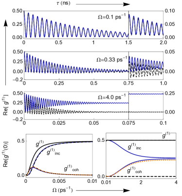
Figure 1: Upper three plots: First order field correlation function for various driving strengths, as indicated, calculated from the full variational theory (blue solid curves), and the pure dephasing approximation of Eqs. (2) and (3) (black dashed curves). The right-most parts show enlargements of the long-time behaviour. Lower plots: Coherent ($g^{(1)}_{\rm coh}$), incoherent ($g^{(1)}_{\rm inc}$), and total ($g^{(1)}$) scattering as a function of driving strength, calculated using the full (blue, solid) and pure dephasing (black, dashed) theories. The total scattering is indistinguishable on this scale between the two models. However, the left plot shows the only region where the pure dephasing model gives a non-negligible coherent contribution, close to the origin; i.e., in the pure dephasing case, all light is incoherently scattered in the right plot. Shown also is $g^{(1)}_{\rm coh}$ calculated from Eq. (4) (orange dotted curve). Parameters: $T_{1}=700~{}\mathrm{ps}$, $\alpha=0.027~{}\mathrm{ps}^{2}$, $\omega_{c}=2.2~{}\mathrm{ps}^{-1}$, and $T=4$ K.

To exemplify the breakdown of the pure-dephasing model, in Fig. 1 we plot $g^{(1)}(\tau)$ calculated using the full variational theory (solid blue curves) and calculated using Eqs. (2) and (3) (black dashed curves). As expected, for weaker driving, $\Omega<0.1~{}\mathrm{ps}^{-1}$, the pure dephasing model gives a good approximation to the full theory. Nevertheless, as the driving strength is increased, significant discrepancies soon become apparent. In particular, from the different long-time values approached when $\Omega\geq 0.33~{}\mathrm{ps}^{-1}$, we conclude that the coherent contribution surprisingly becomes important in this regime, and that this feature is not captured by the pure dephasing approximation. Indeed, when $\Omega=4~{}\mathrm{ps}^{-1}$, the full phonon theory gives $\smash{g^{(1)}_{\rm coh}}\sim 0.25$, in clear distinction to the pure dephasing case.

That Eqs. (2) and (3) cannot capture these effects signifies that above a driving strength of $\Omega\sim 0.1~{}\mathrm{ps}^{-1}$ (for these realistic parameters), the field correlation properties of the QD emission fundamentally depart from the atomic case. At driving above saturation, photons mediate transitions between manifolds of the dot-laser dressed states, while phonons mediate transitions between dressed states in a single manifold. Hence, photon emission acts in this regime to completely suppress QD coherences in the steady-state, while phonons drive thermalisation among the dressed states, thus leading to QD steady-states with non-negligible coherence. When phonon processes dominate over photon emission, as in the strong-driving regime, we then find that the level of coherent emission correspondingly grows. Though the pure dephasing model correctly captures the fact that phonon-induced damping remains driving-dependent across the full parameter range, it fails here because it does not lead to the correct equilibration of the QD with the phonon bath. In this regard, it assumes a high temperature limit with respect to the driving strength, and thus the quantum nature of the environment is lost.

For resonant driving, we can (approximately) rectify this by the modification $\mathcal{K}_{\mathrm{ph}}(\rho_{\rm V})\approx(1/2)\gamma_{\rm PD}(\sigma_{z}\rho_{\rm V}\sigma_{z}-\rho_{\rm V})+(i/4)\kappa[\sigma_{y},\{\sigma_{z},\rho_{\rm V}\}]$, where $\kappa=(\Omega_{r}/2)^{2}\int_{-\infty}^{\infty}\sin(\Omega_{r}s)(\mathrm{e}^{\phi(s)}-\mathrm{e}^{-\phi(s)})\mathrm{d}s$, such that $\kappa/\gamma_{\rm PD}=\tanh(\beta\Omega_{r}/2)$. We now find

$$g^{(1)}_{\mathrm{coh}}\rightarrow G^{(1)}_{\mathrm{coh}}=\left(\frac{\Gamma_{1}\Omega_{r}}{2\Gamma_{1}\Gamma_{2}+2\Omega_{r}^{2}}\right)^{2}+\left(\frac{\Omega_{r}\kappa/\Omega}{\Gamma_{1}+2\gamma_{\rm PD}}\right)^{2},$$ (4)

where the first term is precisely the contribution in the strict pure-dephasing case [see Eq. (3)], which quickly becomes negligible for large $\Omega_{r}$. Conversely, the second term, now arising due to equilibration with the quantum mechanical phonon bath, becomes important as $\Omega_{r}$ increases. To see this, we note that once $\Omega_{r}$ is large enough such that $\Gamma_{1}\ll\gamma_{\rm PD}$, we can approximate $G^{(1)}_{\mathrm{coh}}\approx(\Omega_{r}\tanh(\beta\Omega_{r}/2)/2\Omega)^{2}$. In the upper three plots of Fig. 1, increasing the driving moves the QD from an effective high temperature regime, where $\beta\Omega_{r}\ll 1$ and $G^{(1)}_{\mathrm{coh}}\approx 0$, to an effective low temperature regime, where $\beta\Omega_{r}\gg 1$ and $G^{(1)}_{\mathrm{coh}}\approx(\Omega_{r}/2\Omega)^{2}$. These observations are borne out in the lower part of Fig. 1, where we plot the coherent, incoherent, and total scattering as a function of $\Omega$. The lower left plot shows the region close to the origin, the only regime in which the pure dephasing model predicts a non-negligible level of coherent emission. From the lower right plot, we see also that as the total scattering is fixed at strong driving, the incoherent contribution decreases in our full phonon model as the coherent contribution increases. Again, this is not captured by the pure dephasing treatment. In fact, this represents a hitherto unexplored regime of resonance fluorescence at strong driving, in which both significant coherent scattering and a well-defined Mollow triplet can coexist.

QD resonance fluorescence experiments are usually performed at Rabi frequencies up to around $25$ GHz ($\Omega=0.16$ ps^-1), at which point the coherent fraction is of order $1$ % from our full phonon model, compared to $0.01$ % in the pure dephasing model (for the parameters of Fig. 1). Increasing $\Omega$ fourfold, around 15 % of the light is then coherently scattered in the full model, compared to less than 0.0003 % in the pure dephasing case. Reducing the temperature to $2$ K, the coherent fraction could be increased to about 35 % at this driving strength.

Spectrum.– We now turn our attention to the QD emission spectrum, concentrating on cases where the incoherent contribution dominates (i.e. relatively weak driving), and Eq. (2) is thus approximately valid on resonance. From a Fourier transform of Eq. (2), we find that the resonant Mollow sideband widths are determined by $\Gamma_{1}+\Gamma_{2}=(3/2)\Gamma_{1}+\gamma_{\rm PD}$, with approximate positions $\pm\Omega_{r}$. We therefore expect a systematic broadening and splitting with increasing driving strength Ulrich et al. (2011); Roy and Hughes (2011). Off resonance, we might then also expect sideband broadening and splitting with increasing detuning $\epsilon$ (for fixed $\Omega$) if we were to replace $\Omega_{r}$ with the generalised Rabi frequency, $\Omega_{r}^{\prime}=\sqrt{\Omega_{r}^{2}+\epsilon^{2}}$ Ulrich et al. (2011), leading to similar trends for increasing $\epsilon$ as for $\Omega$. However, the experiments of Ref. Ulrich et al. (2011) showed a systematic narrowing of the Mollow sidebands with increasing detuning, leaving open the question as to why this might be the case.

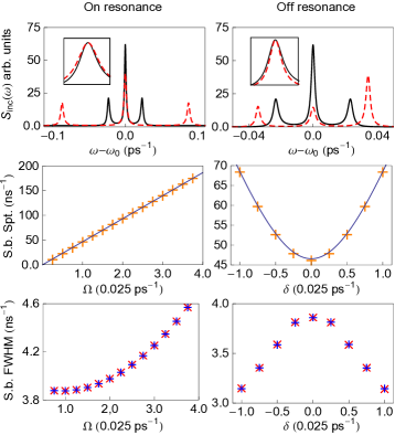
Figure 2: From top to bottom, incoherent emission spectrum, extracted sideband splitting, and extracted sideband width for varying driving strength on resonance (left), and varying detuning (right). The solid black curves in the emission spectra are for $\epsilon=0$, and a driving strength of $\Omega=0.025~{}\mathrm{ps}^{-1}$ (which sets our x-axis units in the rest of the plots). The dashed red curves are for $\Omega=0.094~{}\mathrm{ps}^{-1}$ on resonance, and $\epsilon=\Omega=0.025~{}\mathrm{ps}^{-1}$ off resonance (which has been enhanced by a factor of $5$). The insets show the red sidebands shifted and rescaled to lie on top of each other. The solid blue curves in the middle row show the functions $2\Omega_{r}$ (left) and $2\sqrt{\Omega_{r}^{2}+\epsilon^{2}}$ (right). The symbols in the bottom row correspond to the red ($\times$) and blue ($+$) sidebands. Parameters: $T_{1}=400~{}\mathrm{ps}$, $\alpha=0.027~{}\mathrm{ps}^{2}$, $\omega_{c}=2.2~{}\mathrm{ps}^{-1}$, and $T=10$ K.

In fact, off-resonance the expressions for the spectrum become significantly more complicated than in the resonant case, and the above simple reasoning does not hold. To illustrate this, in Fig. 2, from top to bottom, we plot the incoherent emission spectrum, extracted sideband splitting, and extracted full-width-half-maximum ($=\Gamma$) of the Mollow sidebands, calculated from the full phonon theory. In the latter two cases, the spectrum is fitted by a sum of three Lorentzian functions of the form $L(\omega)=0.5\Gamma/[(\omega-\omega_{p})^{2}+(0.5\Gamma)^{2}]$. The left column corresponds to varying the driving frequency on resonance, while the right column corresponds to varying the detuning with a fixed driving strength.

As can be seen by the sideband splittings in the middle left plot, increasing the driving strength on resonance does, as expected, cause the sidebands to move apart linearly with $\Omega$. Also, we see in the middle right plot that moving off-resonance appears to alter the sideband splitting in exact accordance with the simple procedure of replacing $\Omega_{r}\to\sqrt{\Omega_{r}^{2}+\epsilon^{2}}$. The extracted sideband widths in the lower plots, however, reveal something quite different. On resonance, in accordance with $\gamma_{\rm PD}\sim\Omega_{r}^{2}$, we see a systematic broadening of the sidebands with increasing driving strength. In contrast, as we move off-resonance, we now see a systematic narrowing of the sidebands, consistent with recent experimental results Ulrich et al. (2011). To further confirm this point, the insets of the plots in the top row show the red sidebands in each case plotted on top of each other. We can gain some approximate analytical insight into this behaviour for small detuning by again considering the pure dephasing limit. Allowing for off-resonant driving, we expand the sideband widths to second order in the detuning, from which we find that they are determined by $(3/2)\Gamma_{1}+\gamma_{\rm PD}-(\epsilon/\sqrt{2}\Omega_{r})^{2}(\Gamma_{1}-2\gamma_{\rm PD})$. Hence, for $\Gamma_{1}>2\gamma_{\rm PD}$, as in Fig. 2, we expect narrowing as we detune from resonance, while broadening occurs for $\Gamma_{1}<2\gamma_{\rm PD}$. Note that while we do not include detailed cavity effects here, which give rise to qualitatively different behaviour in Refs. Roy and Hughes (2011, 2012), our results demonstrate that for a QD TLS at least, an increase in sideband splitting off-resonance does not necessarily imply an associated phonon-induced increase in sideband width.

Summary.– We have shown that the balance of coherent to incoherent emission from a driven TLS can be fundamentally altered by environmental interactions, leading to a nonstandard regime of resonance fluorescence attainable in solid-state emitters. In the context of driven QDs, enhanced coherent scattering can occur with increasing driving strength, due to thermalisation in the QD steady-state with respect to the phonon bath. This mechanism is in fact rather general, and could occur for any emitter in which the steady-state becomes dominated by dressed state thermalisation. For off-resonant driving, we have shown that QD-phonon interactions do not necessarily lead to broadening in the spectral sideband widths with increasing detuning. In fact, narrowing can occur in certain regimes, consistent with an observed experimental trend Ulrich et al. (2011). Again, this behaviour is not QD-specific, and so we expect the emission features outlined above to be of importance in a wide variety of experimental settings.

Acknowledgments - During the completion of this work we became aware of similar results for the spectral narrowing obtained independently Ulhaq et al. (2013). We thank Stephen Hughes and co-workers for bringing these to our attention. We also thank Clemens Matthiesen, Brendon Lovett, Erik Gauger, and Sean Barrett for fruitful discussions. D.P.S.M. acknowledges support from the EPSRC, CHIST-ERA project SSQN, and CONICET. A.N. is supported by Imperial College.

I Supplemental Material

In this supplement we outline the derivation of the master equation used in the main text, Eq. (1). We first show how the quantum dot-phonon and quantum dot-photon coupling effects can be treated independently within our formalism. We then give expressions from the variational method used to treat the quantum dot-phonon coupling, and show how they can be approximated by a pure dephasing form in the appropriate (weak-driving) limit.

I.1 Separation of phonon and photon terms

Our starting point is the quantum dot (QD) Hamiltonian as given in the main text:

$$H=\nu|X\rangle\langle X|+\frac{\Omega}{2}\sigma_{x}+\sum_{\bf k}\omega_{\bf k}b_{\bf k}^{\dagger}b_{\bf k}+|X\rangle\langle X|\sum_{\bf k}g_{\bf k}(b_{\bf k}^{\dagger}+b_{\bf k})+\sum_{\bf q}\eta_{\bf q}a_{\bf q}^{\dagger}a_{\bf q}+\sum_{\bf q}(h_{\bf q}a_{\bf q}\sigma_{+}e^{i\omega_{l}t}+{h^{*}_{\bf q}}a_{\bf q}^{\dagger}\sigma_{-}e^{-i\omega_{l}t}).$$ (5)

Following Ref. McCutcheon et al. (2011), we first apply a unitary variational transformation in order to treat the QD-phonon interaction beyond the weak coupling approximation. The transformed Hamiltonian is defined by $H_{V}=e^{V}He^{-V}$, where

$$\exp[\pm V]=\exp\bigg{[}\pm|X\rangle\langle X|\sum_{\bf k}(\alpha_{\bf k}b_{\bf k}^{\dagger}-\alpha_{\bf k}^{*}b_{\bf k})\bigg{]}=|0\rangle\langle 0|+|X\rangle\langle X|\prod_{\bf k}D(\pm\alpha_{\bf k}),$$ (6)

with $D(\pm\alpha_{\bf k})=\exp[\pm(\alpha_{\bf k}b_{\bf k}^{\dagger}-\alpha_{\bf k}^{*}b_{\bf k})]$ and $\alpha_{\bf k}=f_{\bf k}/\omega_{\bf k}$. Here, $f_{\bf k}$ are variational parameters to be determined later. After the transformation, we write $H_{V}=H_{S}+H_{1a}+H_{1b}+H_{12}+H_{B_{1}}+H_{B_{2}}$, where

$$H_{S}=\frac{R}{2}\openone+\frac{\epsilon}{2}\sigma_{z}+\frac{\Omega_{r}}{2}\sigma_{x},$$ (7)

and the interaction terms $H_{1a}=|X\rangle\langle X|\sum_{\bf k}(g_{\bf k}-f_{\bf k})(b_{\bf k}^{\dagger}+b_{\bf k})$ and $H_{1b}=\frac{\Omega}{2}\left(\sigma_{x}B_{x}+\sigma_{y}B_{y}\right)$, with $B_{x}=\frac{1}{2}(B_{+}+B_{-}-2B)$ and $B_{y}=\frac{1}{2i}(B_{-}-B_{+})$ for $B_{\pm}=\prod_{\bf k}D(\pm\alpha_{\bf k})$, contain only QD and phonon operators. The interaction term

$$H_{12}=\sum_{\bf q}(h_{\bf q}a_{\bf q}B_{+}\sigma_{+}e^{i\omega_{l}t}+{h^{*}_{\bf q}}a_{\bf q}^{\dagger}B_{-}\sigma_{-}e^{-i\omega_{l}t}),$$ (8)

contains QD, phonon, and photon operators, and the bath Hamiltonians are $H_{B_{1}}=\sum_{\bf k}\omega_{\bf k}b_{\bf k}^{\dagger}b_{\bf k}$ and $H_{B_{2}}=\sum_{\bf q}\eta_{\bf q}a_{\bf q}^{\dagger}a_{\bf q}$. The detuning now becomes $\epsilon=\omega_{0}^{\prime}-\omega_{l}$, defined in terms of the bath-shifted QD transition energy $\omega_{0}^{\prime}=\omega_{0}+R$, with $R=\sum_{\bf k}\omega_{\bf k}^{-1}f_{\bf k}(f_{\bf k}-2g_{\bf k})$. We assume a thermal equilibrium state for the phonon and photon baths, $\rho_{B}=e^{-\beta H_{B}}/{\rm tr}_{B}(e^{-\beta H_{B}})=[e^{-\beta H_{B_{1}}}/{\rm tr}_{B_{1}}(e^{-\beta H_{B_{1}}})][e^{-\beta H_{B_{2}}}/{\rm tr}_{B_{2}}(e^{-\beta H_{B_{2}}})]=\rho_{B_{1}}\rho_{B_{2}}$, and in doing so find that the operators $B_{\pm}$ have the same average with respect to this state: $B=\rm{tr}(B_{\pm}\rho_{B})=\exp[-(1/2)\sum_{\bf k}|\alpha_{\bf k}|^{2}\coth{(\beta\omega_{\bf k}/2)}]$, with inverse temperature $\beta=1/(k_{B}T)$. The bath-renormalised Rabi frequency is defined as $\Omega_{r}=B\Omega$.

We now separate the variationally-transformed Hamiltonian into $H_{V}=H_{0}+H_{I}$, with $H_{0}=H_{S}+H_{B_{1}}+H_{B_{2}}$ and $H_{I}=H_{1a}+H_{1b}+H_{12}$, and treat $H_{I}$ as a perturbation. We move into the interaction picture with respect to $H_{0}$, yielding an interaction Hamiltonian in the (variationally-transformed) interaction picture of the form $\tilde{H}_{I}(t)=\tilde{H}_{1a}(t)+\tilde{H}_{1b}(t)+\tilde{H}_{12}(t)$, where $\tilde{H}_{1a}(t)=e^{iH_{0}t}H_{1a}e^{-iH_{0}t}$, $\tilde{H}_{1b}(t)=e^{iH_{0}t}H_{1b}e^{-iH_{0}t}$, and

$$\tilde{H}_{12}(t)=e^{iH_{0}t}H_{12}e^{-iH_{0}t}=\sum_{\bf q}(h_{\bf q}a_{\bf q}e^{-i\eta_{\bf q}t}B_{+}(t)\sigma_{+}(t)e^{i\omega_{l}t}+{h^{*}_{\bf q}}a_{\bf q}^{\dagger}e^{i\eta_{\bf q}t}B_{-}(t)\sigma_{-}(t)e^{-i\omega_{l}t}).$$ (9)

Here, $B_{\pm}(t)=e^{iH_{B_{1}}t}B_{\pm}e^{-iH_{B_{1}}t}=\prod_{\bf k}D(\pm\alpha_{\bf k}e^{i\omega_{\bf k}t})$, and

$$\sigma_{\pm}(t)e^{\pm i\omega_{l}t}=\exp\Big{[}i\Big{(}\frac{\epsilon}{2}\sigma_{z}+\frac{\Omega_{r}}{2}\sigma_{x}\Big{)}t\Big{]}\sigma_{\pm}\exp\Big{[}-i\Big{(}\frac{\epsilon}{2}\sigma_{z}+\frac{\Omega_{r}}{2}\sigma_{x}\Big{)}t\Big{]}e^{\pm i(\omega_{0}-\nu)t}.$$ (10)

Provided $\omega_{0}\gg\nu,\epsilon,\Omega_{r}$, which is generally the case for driven QDs since $\omega_{0}\sim 1$ eV compared to meV or smaller energy scales for the other quantities, we can then approximate $\sigma_{\pm}(t)e^{\pm i\omega_{l}t}\approx\sigma_{\pm}e^{\pm i\omega_{0}t}$.

Following the standard projection-operator procedure we derive a time-local master equation for the reduced QD exciton density operator, $\tilde{\rho}_{V}$, in the variational frame interaction picture. Choosing the bath reference state to be $\rho_{B}$ used above, we find

$$\frac{\rm{d}\tilde{\rho}_{V}(t)}{\rm{d}t}=-\int_{0}^{t}\mathrm{d}s{\rm tr}_{B}[\tilde{H}_{I}(t),[\tilde{H}_{I}(s),\tilde{\rho}_{V}(t)\rho_{B}]].$$ (11)

Since ${\rm{tr}}_{B_{1}}(\tilde{H}_{1a}(t)\rho_{B_{1}})={\rm{tr}}_{B_{1}}(\tilde{H}_{1b}(t)\rho_{B_{1}})={\rm{tr}}_{B_{2}}(\tilde{H}_{12}(t)\rho_{B_{2}})=0$, we find that Eq. (11) can be written $\frac{d\tilde{\rho}_{V}(t)}{dt}=\tilde{\mathcal{K}}_{\mathrm{ph}}(\tilde{\rho}_{V}(t))+\tilde{\mathcal{K}}_{\mathrm{sp}}(\tilde{\rho}_{V}(t))$, where

$$\tilde{\mathcal{K}}_{\mathrm{ph}}(\tilde{\rho}_{V}(t))=-\int_{0}^{t}\mathrm{d}s{\rm tr}_{B_{1}}[\tilde{H}_{1a}(t)+\tilde{H}_{1b}(t),[\tilde{H}_{1a}(s)+\tilde{H}_{1b}(s),\tilde{\rho}_{V}(t)\rho_{B_{1}}]]$$ (12)

and is precisely the form expected from the variational treatment of QD exciton-phonon interactions in the absence of the radiation field, whereas

$$\tilde{\mathcal{K}}_{\mathrm{sp}}(\tilde{\rho}_{V}(t))=-\int_{0}^{t}\mathrm{d}s{\rm tr}_{B_{1}+B_{2}}[\tilde{H}_{12}(t),[\tilde{H}_{12}(s),\tilde{\rho}_{SP}(t)\rho_{B_{1}}\rho_{B_{2}}]],$$ (13)

is responsible for photon emission and absorption processes. Though the latter term appears at this stage to be modified by the phonon environment due to our use of the variational transformation, we shall now show that the modification is negligible for the situation considered in this work.

I.2 Spontaneous emission terms

To proceed, we write $\tilde{H}_{12}(t)=A(t)Q(t)B_{+}(t)+(A(t)Q(t)B_{+}(t))^{\dagger}$, with $A(t)=\sigma_{+}e^{i\omega_{0}t}$ and $Q(t)=\sum_{\bf q}h_{\bf q}a_{\bf q}e^{-i\eta_{\bf q}t}$, where $A(t)$, $Q(t)$, and $B_{+}(t)$ all commute. Inserting this into Eq. (13), we find that the radiation field term can be written in the simple and familiar form

$$\tilde{\mathcal{K}}_{\mathrm{sp}}(\tilde{\rho}_{V}(t))=\Gamma_{1}(t)\left(\sigma_{-}\tilde{\rho}_{V}(t)\sigma_{+}-\frac{1}{2}\{\sigma_{+}\sigma_{-},\tilde{\rho}_{V}(t)\}\right).$$ (14)

where we ignore absorption and stimulated emission processes under the assumption that no thermal photons exist at the appropriate energy scale for temperatures of interest. Additionally, we have ignored the Lamb-shift of the excitonic energy splitting induced by the radiation field. The rate of spontaneous emission processes is given by

$$\Gamma_{1}(t)=2{\rm Re}\int_{0}^{t}\mathrm{d}\tau e^{i\omega_{0}\tau}C(\tau)X(\tau),$$ (15)

where in the continuum limit of the phonon bath

$$C(\tau)={\rm{tr}}_{B_{1}}(B_{\pm}(\tau)B_{\mp})=\exp{\bigg{[}-\int_{0}^{\infty}\mathrm{d}\omega\frac{J_{\mathrm{ph}}(\omega)}{\omega^{2}}F(\omega)^{2}((1-\cos{\omega\tau})\coth{\beta\omega/2}+i\sin{\omega\tau})\bigg{]}},$$ (16)

with $f_{\bf k}/g_{\bf k}=F(\omega_{\bf k})$ (which will be justified later), and $J_{\mathrm{ph}}(\omega)=\sum_{\bf k}|g_{\bf k}|^{2}\delta(\omega-\omega_{\bf k})$ is the phonon spectral density. In the continuum limit of the photon bath $X(\tau)=\int_{0}^{\infty}\mathrm{d}\eta e^{-i\eta\tau}J_{\mathrm{pt}}(\eta)$, where $J_{\mathrm{pt}}(\eta)=\sum_{\bf q}|h_{\bf q}|^{2}\delta(\eta-\eta_{\bf q})$ is the relevant photon spectral density. Thus, the spontaneous emission rate we derive within the variational theory is dependent upon both the phonon and photon bath correlation functions, $C(\tau)$ and $X(\tau)$, respectively, and whether this rate varies from that in the absence of the phonon environment depends crucially on their respective timescales.

We know that the typical timescale for the phonon-bath correlation function to reach the long-time value of $B^{2}$ is of the order of a few picoseconds Ramsay et al. (2010a, b). For $X(\tau)$, we take the standard (3D) spectral density $J_{\rm{pt}}(\eta)=A\,\eta^{3}e^{-\eta/\eta_{c}}$, where a high-frequency cut-off $\eta_{c}$ has been introduced. This gives

$$X(\tau)=\frac{6A}{(\eta_{c}^{-1}+i\tau)^{4}},$$ (17)

which decays to zero on a timescale of roughly $1/\eta_{c}$. For spontaneous emission not to be suppressed, it must be the case that $\eta_{c}>\omega_{0}$. Thus, we can estimate $\eta_{c}>1.5\times 10^{3}$ ps^-1, for a typical $|0\rangle$ to $|X\rangle$ energy splitting of $1$ eV, which leads to a radiation field correlation time of the order of femtoseconds at most. On this timescale, the phonon correlation function barely changes, and we may replace $C(\tau)$ by $C(0)=1$ in Eq. (15), and we are also now justified in taking the upper limit of integration to infinity for timescales of interest. Thus, for a typical QD system as described in the main text, the spontaneous emission process is unaltered by the exciton-phonon coupling, and can be described by the standard Lindblad form of Eq. (14) with $\Gamma_{1}(t)$ replaced with $\Gamma_{1}=2\pi J_{\rm{pt}}(\omega_{0})$.

I.3 Phonon coupling terms

We now use the methods described in Ref. McCutcheon et al. (2011) to find the form of the phonon terms. The variational parameters upon which $H_{1a}$, $H_{1b}$ and $H_{S}$ all depend are found by minimising a free energy bound on the interaction terms. We find $f_{\bf k}=g_{\bf k}F(\omega_{\bf k})$ with

$$F(\omega_{\bf k})=\frac{(1-\frac{\epsilon}{\xi}\tanh(\beta\xi/2))}{1-\frac{\epsilon}{\xi}\tanh(\beta\xi/2)\Big{(}1-\frac{\Omega_{r}^{2}}{2\epsilon\omega_{\bf k}}\coth(\beta\omega_{\bf k}/2)\Big{)}},$$ (18)

and $\xi=\sqrt{\Omega^{2}+\epsilon^{2}}$. We note that since $\Omega_{r}=\Omega B$ and $\epsilon=\nu+R$ are functions of $F(\omega_{\bf k})$ their values must be solved for self-consistently.

Moving the phonon coupling terms back into the Schrödinger picture, $\mathcal{K}_{\rm{ph}}(\rho_{V}(t))=\mathrm{e}^{-iH_{0}t}\tilde{\mathcal{K}}_{\mathrm{ph}}(\tilde{\rho}_{V}(t))\mathrm{e}^{iH_{0}t}$, we find

$$\mathcal{K}_{\rm{ph}}(\rho_{V}(t))= -{\textstyle{\frac{1}{2}}}\sum_{ij}\sum_{\omega}\gamma_{ij}(\omega)[A_{i},A_{j}(\omega)\rho_{V}(t)-\rho_{V}(t)A_{j}^{\dagger}(\omega)]$$

$$-i\sum_{ij}\sum_{\omega}S_{ij}(\omega)[A_{i},A_{j}(\omega)\rho_{V}(t)+\rho_{V}(t)A_{j}^{\dagger}(\omega)],$$ (19)

where $\{i,j\}\in\{1,2,3\}$ and $\omega\in\{0,\pm\xi\}$. We define $A_{1}=\sigma_{x}$, $A_{2}=\sigma_{y}$ and $A_{3}=(1/2)(I+\sigma_{z})$, while $A_{1}(0)=\sin 2\theta(\left|+\right\rangle\hskip-2.84526pt\left\langle+\right|-\left|-\right\rangle\hskip-2.84526pt\left\langle-\right|)$, $A_{1}(\xi)=\cos 2\theta\left|-\right\rangle\hskip-2.84526pt\left\langle+\right|$, $A_{2}(0)=0$, $A_{2}(\xi)=i\left|-\right\rangle\hskip-2.84526pt\left\langle+\right|$, $A_{3}(0)=\cos^{2}\theta\left|+\right\rangle\hskip-2.84526pt\left\langle+\right|+\sin^{2}\theta\left|-\right\rangle\hskip-2.84526pt\left\langle-\right|$ and $A_{3}(\xi)=-\sin\theta\cos\theta\left|-\right\rangle\hskip-2.84526pt\left\langle+\right|$, defined in terms of the eigenstates of $H_{S}$, satisfying $H_{S}\left|\pm\right\rangle=(1/2)(R\pm\xi)\left|\pm\right\rangle$. In all cases $A_{i}(\omega)=A_{i}^{\dagger}(-\omega)$, and $\theta=(1/2)\arctan(\Omega_{r}/\epsilon)$. Eq. (19) contains the quantities $\gamma_{ij}(\omega)=2\mathrm{Re}[K_{ij}(\omega)]$ and $S_{ij}(\omega)=\mathrm{Im}[K_{ij}(\omega)]$, defined in terms of the response functions

$$K_{ij}(\omega)=\int_{0}^{\infty}\Lambda_{ij}(\tau)\mathrm{e}^{i\omega t}\mathrm{d}\tau,$$ (20)

which themselves depend on the bath correlation functions $\Lambda_{ij}(\tau)=\mathrm{tr}(\tilde{B}_{i}(\tau)\tilde{B}_{j}(0)\rho_{B})$. Note that in Eq. (20) we have extended the upper limit of integration to infinity which, for the parameters considered in the main text, is a good approximation McCutcheon and Nazir (2010). We label the bath operators $B_{1}=(\Omega/2)B_{x}$, $B_{2}=(\Omega/2)B_{y}$, and $B_{3}=\sum_{\bf k}(g_{\bf k}-f_{\bf k})(b_{\bf k}^{\dagger}+b_{\bf k})$. The bath correlation functions are found to be $\Lambda_{11}(\tau)=(\Omega_{r}^{2}/8)(\mathrm{e}^{\phi(\tau)}+\mathrm{e}^{-\phi(\tau)}-2)$ and $\Lambda_{22}(\tau)=(\Omega_{r}^{2}/8)(\mathrm{e}^{\phi(\tau)}-\mathrm{e}^{-\phi(\tau)})$, with phonon propagator

$$\phi(\tau)=\int_{0}^{\infty}\mathrm{d}\omega\frac{J(\omega)}{\omega^{2}}F(\omega)^{2}G_{+}(\tau),$$ (21)

defined in terms of $G_{\pm}(\tau)=(n(\omega)+1)e^{-i\omega\tau}\pm n(\omega)\mathrm{e}^{i\omega\tau}$, with $n(\omega)=(e^{\beta\omega}-1)^{-1}$ the occupation number, while

$$\Lambda_{33}(\tau)=\int_{0}^{\infty}\mathrm{d}\omega J(\omega)(1-F(\omega))^{2}G_{+}(\tau),\qquad\Lambda_{32}(\tau)=\frac{\Omega_{r}}{2}\int_{0}^{\infty}\mathrm{d}\omega\frac{J(\omega)}{\omega}F(\omega)(1-F(\omega))iG_{-}(\tau),$$ (22)

with $\Lambda_{32}(\tau)=-\Lambda_{23}(\tau)$, and $\Lambda_{12}(\tau)=\Lambda_{21}(\tau)=\Lambda_{13}(\tau)=\Lambda_{31}(\tau)=0$.

Putting everything together, we arrive at the full variational frame Schrödinger picture master equation

$$\frac{\rm{d}\rho_{V}(t)}{\rm{d}t}=-\frac{i}{2}[\epsilon\sigma_{z}+\Omega_{r}\sigma_{x},\rho_{V}(t)]+\mathcal{K}_{\rm{ph}}(\rho_{V}(t))+\Gamma_{1}\left(\sigma_{-}\rho_{V}(t)\sigma_{+}-\frac{1}{2}\{\sigma_{+}\sigma_{-},\rho_{V}(t)\}\right),$$ (23)

as used in the main text. We note that in moving the spontaneous emission terms back into the Schrödinger picture the QD operators $\sigma_{\pm}$ have remained unchanged to be consistent with the approximation that $\sigma_{\pm}(t)e^{\pm i\omega_{l}t}\approx\sigma_{\pm}e^{\pm i\omega_{0}t}$ used previously.

I.4 Pure dephasing limit

Though we use the full form of Eq. (19) for the phonon coupling in numerically calculating the field correlation properties of the QD, the analytical expressions resulting from it are somewhat cumbersome. However, in the correct (weak-driving) limit, we find that the phonon coupling terms in Eq. (19) can be well approximated by a simple pure dephasing form. Assuming now that we drive the QD on resonance with the polaron shifted transition frequency, $\nu-\sum_{\bf k}\omega^{-1}g_{\bf k}^{2}=0$, and we drive weakly enough such that $\Omega\ll\omega_{c}$, then the variational transformation reduces approximately to the full polaron form, and we can thus set $F(\omega_{\bf k})\approx 1$ in Eq. (18). As such, we find that only the correlation functions $\Lambda_{11}(\tau)$ and $\Lambda_{22}(\tau)$ survive, and the variational master equation (now ignoring spontaneous emission) reduces to the polaron form given in Ref. McCutcheon and Nazir (2010). This corresponds to Bloch equations of the form $\dot{\boldsymbol{\alpha}}=M\cdot\boldsymbol{\alpha}+\boldsymbol{b}$, where

$$M=\left(\begin{array}[]{ccc}-(\Gamma_{z}-\Gamma_{y})&0&0\\ 0&-\Gamma_{y}&-\Omega_{r}\\ 0&(\Omega_{r}+\lambda)&-\Gamma_{z}\end{array}\right),$$ (24)

and $\boldsymbol{b}=(-\kappa_{x},0,0)^{T}$, with Bloch vector $\boldsymbol{\alpha}=(\langle\sigma_{x}\rangle_{t},\langle\sigma_{y}\rangle_{t},\langle\sigma_{z}\rangle_{t})^{T}$. The rates and energy shifts are given by $\Gamma_{y}=2\gamma_{11}(0)$, $\Gamma_{z}=\gamma_{22}(\Omega_{r})+\gamma_{22}(-\Omega_{r})$, $\kappa=\gamma_{22}(\Omega_{r})-\gamma_{22}(-\Omega_{r})$, and $\lambda=2[S_{22}(\Omega_{r})-S_{22}(-\Omega_{r})]$. We are interested in the solutions to these Bloch equations for arbitrary initial conditions as, with the help of the regression theorem, this will determine the phonon contribution to the first-order field correlation function, and hence the QD emission spectrum. For the appropriate phonon spectral density used in the main text, $J_{\rm{ph}}(\omega)=\alpha\,\omega^{3}\exp[-(\omega/\omega_{c})^{2}]$, we find that in the regime that $k_{B}T<\omega_{c}$, as the driving strength becomes small, then $\gamma_{11}(0)$ becomes negligible in comparison to $\gamma_{22}(\pm\Omega_{r})$. Hence, $\Gamma_{y}\rightarrow 0$, while $\Gamma_{z}\rightarrow(\gamma_{22}(\Omega_{r})+\gamma_{22}(-\Omega_{r}))$. Additionally, $\lambda\ll\Omega_{r}$ in this regime, and $(\Gamma_{z}-\Gamma_{y})/\zeta\approx\Gamma_{z}/\sqrt{\Omega_{r}^{2}-(1/4)\Gamma_{z}^{2}}$ is very small as well. If we additionally impose $\Omega\beta\ll 1$, such that $\kappa/\Gamma_{z}\rightarrow 0$, then we may approximate the Bloch equation solutions as

$$\langle\sigma_{x}\rangle_{t} {}\approx{} e^{-\Gamma_{z}t}\langle\sigma_{x}\rangle_{0},$$ (25)

$$\langle\sigma_{y}\rangle_{t} {}\approx{} e^{-\Gamma_{z}t/2}\left[\langle\sigma_{y}\rangle_{0}\cos{(\zeta t)}-\frac{\Omega_{r}}{\zeta}\langle\sigma_{z}\rangle_{0}\sin{(\zeta t)}\right],$$ (26)

$$\langle\sigma_{z}\rangle_{t} {}\approx{} e^{-\Gamma_{z}t/2}\left[\langle\sigma_{z}\rangle_{0}\cos{(\zeta t)}+\frac{\Omega_{r}}{\zeta}\langle\sigma_{y}\rangle_{0}\sin{(\zeta t)}\right],$$ (27)

where $\zeta\rightarrow\sqrt{\Omega_{r}^{2}-(1/4)\Gamma_{z}^{2}}$. Now, if we identify $\gamma_{PD}=\Gamma_{z}$, then these are precisely the solutions we expect from a simple pure dephasing master equation of the form

$$\dot{\rho}=-\frac{i\Omega_{r}}{2}[\sigma_{x},\rho]+\frac{\gamma_{PD}}{2}(\sigma_{z}\rho\sigma_{z}-\rho),$$ (28)

in the relevant regime of $\gamma_{PD}/\sqrt{\Omega_{r}^{2}-(1/4)\gamma_{PD}^{2}}$ being small. Furthermore, if we wish to ensure that the system tends to the correct steady state in the long-time limit, we then need to add a term $(i\kappa/4)[\sigma_{y},\{\sigma_{z},\rho\}]$ to the right-hand-side of Eq. (28), such that the solution for $\langle\sigma_{x}\rangle_{t}$ becomes $\langle\sigma_{x}\rangle_{t}=\frac{e^{-\Gamma_{z}t}}{\Gamma_{z}}\left[\langle\sigma_{x}\rangle_{0}\Gamma_{z}+\kappa\right]-\frac{\kappa}{\Gamma_{z}}$. This justifies the forms given in the main text for weak driving, and is further confirmed by the agreement we see with the full numerical solution of the variational master equation in the appropriate regimes.

References

Mollow (1969)
B. R. Mollow,
Phys. Rev. 188,
1969 (1969).
Carmichael (1998)
H. J. Carmichael,
Statistical Methods in Quantum Optics
(Springer, New York, 1998).
Schuda et al. (1974)
F. Schuda,
C. R. Stroud Jr,
and M. Hercher,
J. Phys. B 7,
L198 (1974).
Xu et al. (2007)
X. Xu et al.,
Science 317,
929 (2007).
Muller et al. (2007)
A. Muller et al.,
Phys. Rev. Lett. 99,
187402 (2007).
Ates et al. (2009)
S. Ates et al.,
Phys. Rev. Lett. 103,
167402 (2009).
Flagg et al. (2009)
E. B. Flagg
et al., Nature Phys.
5, 203 (2009).
Vamivakas et al. (2009)
A. N. Vamivakas
et al., Nature Phys.
5, 198 (2009).
Ulrich et al. (2011)
S. M. Ulrich
et al., Phys. Rev. Lett.
106, 247402
(2011).
Ulhaq et al. (2012)
A. Ulhaq et al.,
Nature Photon. 6,
238 (2012).
Wrigge et al. (2008)
G. Wrigge et al.,
Nature Phys. 4,
60 (2008).
Astafiev et al. (2010)
O. Astafiev
et al., Science
327, 840 (2010).
Zrenner et al. (2002)
A. Zrenner et al.,
Nature 418,
612 (2002).
Ramsay et al. (2010a)
A. J. Ramsay
et al., Phys. Rev. Lett.
104, 017402
(2010a).
Ramsay et al. (2010b)
A. J. Ramsay
et al., Phys. Rev. Lett.
105, 177402
(2010b).
Michler et al. (2000)
P. Michler et al.,
Science 290,
2282 (2000).
Santori et al. (2001)
C. Santori et al.,
Phys. Rev. Lett. 86,
1502 (2001).
Santori et al. (2002)
C. Santori et al.,
Nature 419,
594 (2002).
Flagg et al. (2010)
E. B. Flagg
et al., Phys. Rev. Lett.
104, 137401
(2010).
Patel et al. (2010)
R. B. Patel
et al., Nature Photon.
4, 632 (2010).
Nguyen et al. (2011)
H. S. Nguyen
et al., Appl. Phys. Lett.
99, 261904
(2011).
Matthiesen et al. (2012)
C. Matthiesen,
A. N. Vamivakas,
and
M. Atatüre,
Phys. Rev. Lett. 108,
093602 (2012).
Konthasinghe et al. (2012)
K. Konthasinghe
et al., Phys. Rev. B
85, 235315
(2012).
Kiraz et al. (2004)
A. Kiraz,
M. Atatüre,
and A. Imamoglu,
Phys. Rev. A 69,
032305 (2004).
Benjamin et al. (2009)
S. Benjamin,
B. Lovett, and
J. M. Smith,
Laser & Photon. Rev. 3,
556 (2009).
Nazir (2008)
A. Nazir,
Phys. Rev. B 78,
153309 (2008).
Machnikowski and Jacak (2004)
P. Machnikowski
and L. Jacak,
Phys. Rev. B. 69,
193302 (2004).
Vagov et al. (2007)
A. Vagov et al.,
Phys. Rev. Lett. 98,
227403 (2007).
McCutcheon and Nazir (2010)
D. P. S. McCutcheon
and A. Nazir,
New J. Phys. 12,
113042 (2010).
Roy and Hughes (2011)
C. Roy and
S. Hughes,
Phys. Rev. Lett. 106,
247403 (2011).
Roy and Hughes (2012)
C. Roy and
S. Hughes,
Phys. Rev. B 85,
115309 (2012).
Ahn et al. (2005)
K. J. Ahn,
J. Förstner,
and A. Knorr,
Phys. Rev. B 71,
153309 (2005).
Moelbjerg et al. (2012)
A. Moelbjerg
et al., Phys. Rev. Lett.
108, 017401
(2012).
del Valle and Laussy (2010)
E. del Valle and
F. P. Laussy,
Phys. Rev. Lett. 105,
233601 (2010).
Wilson-Rae and Imamoglu (2002)
I. Wilson-Rae and
A. Imamoglu,
Phys. Rev. B 65,
235311 (2002).
McCutcheon et al. (2011)
D. P. S. McCutcheon
et al., Phys. Rev. B
84, 081305(R)
(2011).
Förstner et al. (2003)
J. Förstner
et al., Phys. Rev. Lett.
91, 127401
(2003).
Krugel et al. (2005)
A. Krugel et al.,
Appl. Phys. B. 81,
897 (2005).
Silbey and Harris (1984)
R. Silbey and
R. A. Harris,
J. Chem. Phys. 80,
2615 (1984).
(40)
See the Supplemental Material below for full details of the derivation.
Ulhaq et al. (2013)
A. Ulhaq et al.,
Opt. Express 21,
4382 (2013).