A quenched study of the Schrödinger functional with chirally rotated boundary conditions: non-perturbative tuning

Abstract

The use of chirally rotated boundary conditions provides a formulation of the Schrödinger functional that is compatible with automatic O($a$) improvement of Wilson fermions up to O($a$) boundary contributions. The elimination of bulk O($a$) effects requires the non-perturbative tuning of the critical mass and one additional boundary counterterm. We present the results of such a tuning in a quenched setup for several values of the renormalized gauge coupling, from perturbative to non-perturbative regimes, and for a range of lattice spacings. We also check that the correct boundary conditions and symmetries are restored in the continuum limit.

1 Introduction

The Schrödinger functional of QCD [1, 2, 3] is the gauge invariant functional integral for QCD on a hyper-cylinder where the fields satisfy periodic boundary conditions in the spatial directions and Dirichlet boundary conditions at the Euclidean times $0$ and $T$. The SF is non-perturbatively defined and it has been shown to be very successful when used as a renormalization scheme for lattice QCD. An incomplete set of results obtained using the SF is given by refs. [4, 5, 6, 7, 8, 9, 10, 11, 12].

Because of the Dirichlet boundary conditions in the time direction, the SF has a spectral gap even at zero quark mass [2, 13], thus allowing to use the SF as a massless renormalization scheme. Moreover, due to the possibility of applying finite-size techniques, the SF is an ideal framework to evaluate scale-dependent quantities over a wide range of energies, covering the perturbative up to the non-perturbative regimes. Such a framework is needed when studying non-perturbative renormalization on the lattice. Another good property of the SF is the ability to define gauge invariant quark sources, making it possible to construct gauge invariant correlation functions to determine renormalization factors.

The implementation of the SF on the lattice beyond the pure gauge theory is not a straightforward issue. Depending on the bulk lattice Dirac operator adopted, boundary terms in the lattice action may need to be added in order to recover the correct boundary conditions in the continuum limit. For the implementation with Wilson fermions [2, 3], the boundary conditions arise naturally [13] and no fine-tuning is needed near the boundary. For Ginsparg-Wilson fermions, specific boundary terms have to be added to the lattice action in order to recover the correct continuum limit [13]. A related issue is the definition of boundary conditions in order to achieve automatic O($a$) improvement [14] with massless Wilson quarks. In this case one would like to have boundary conditions in the continuum limit that allow Wilson fermions to maintain automatic O($a$) improvement, similarly to what happens with twisted mass fermions. A solution to this problem has been proposed by Sint [15, 16], called the chirally rotated Schrödinger functional ($\chi$SF). Being compatible with automatic O($a$) improvement, makes the $\chi$SF an ideal setup for renormalizing bare operators computed with Wilson twisted mass fermions at maximal twist [17] and it may have several advantages compared with the standard SF. Here we just mention the possibility of computing renormalization factors of four-fermion operators (like for $B_{K}$) or of twist-2 operators (like for $\langle x\rangle$) free of O($a$) corrections.

The main content of this paper is the numerical investigation of the non-perturbative tuning of the $\chi$SF in a quenched setup. In sect. 2 we start with Wilson twisted mass fermions as an example of automatic O($a$) improvement. Then in sect. 3 we discuss the $\chi$SF in the continuum and its relationship with automatic O($a$) improvement. In sect. 4 we introduce the appropriate lattice action for Wilson fermions and the boundary counterterms and in sect. 5 we discuss the non-perturbative tuning of the critical mass and of the relevant boundary counterterm needed to obtain the correct continuum limit. In sect. 6 we check that the proper symmetries and boundary conditions are recovered in the continuum limit. In a forthcoming paper [18] we will study the application of the $\chi$SF renormalization scheme to the determination of several physically relevant quantities. The computation of such quantities will moreover allow us to perform a continuum limit scaling test for cutoff effects both for small and large volume calculations.

2 Wilson twisted mass fermions and automatic O($a$) improvement

The Wilson twisted mass (Wtm) formulation [19, 20] is a lattice action that provides a solid framework to perform large scale simulations with $N_{f}=0,2$ [21, 22, 17, 23] and more recently $N_{f}=2+1+1$ [24] flavors of dynamical fermions. One of its advantages is the automatic O($a$) improvement of physical correlation functions [14], which requires the non-perturbative tuning of just a single parameter: the critical mass $m_{\rm cr}$. The resulting lattice action is referred to as Wtm at maximal twist. Clearly it would be desirable to retain automatic O($a$) improvement thorugh the process of renormalizing local operators.

We now briefly summarize how automatic O($a$) improvement works for Wilson twisted mass fermions in a finite volume without boundaries. The very same mechanism will be used in the next section to show how the $\chi$SF retains this property. The action for twisted mass QCD (tmQCD) in the continuum for a flavor doublet $\chi$ of fermions is

$$S=\int\!\!d^{4}x~{}\overline{\chi}(x)\left[\gamma_{\mu}\mathcal{D}_{\mu}+m_{\rm q}+i\mu_{\rm q}\gamma_{5}\tau^{3}\right]\chi(x),$$ (2.1)

where $m_{\rm q}$ is the so-called untwisted mass, $\mu_{\rm q}$ the twisted mass and $\tau^{3}$ is the third of the Pauli matrices $\tau^{a}$. Performing the following non-anomalous change of basis

$$\psi(x)={\rm e}^{i\omega\gamma_{5}\tau^{3}/2}\chi(x),\qquad\overline{\psi}(x)=\overline{\chi}(x){\rm e}^{i\omega\gamma_{5}\tau^{3}/2},\qquad\omega=\arctan\left(\frac{\mu_{\rm q}}{m_{\rm q}}\right)\,,$$ (2.2)

it is easy to see that the tmQCD action (2.8) is equivalent to the standard QCD action for degenerate $N_{f}=2$ fermions $\psi$ with mass $M=\sqrt{m_{\rm q}^{2}+\mu_{\rm q}^{2}}$. This trivial change of basis becomes non-trivial once we decide to discretize the QCD action with Wilson fermions obtaining

$$S=a^{4}\sum_{x}\overline{\chi}(x)\left[\mathcal{D}_{W}+m_{0}+i\mu_{\rm q}\gamma_{5}\tau^{3}\right]\chi(x)\,,$$ (2.3)

where $\mathcal{D}_{W}$ is the standard Wilson operator

$$\mathcal{D}_{W}=\frac{1}{2}\left[\left(\nabla_{\mu}+\nabla_{\mu}^{*}\right)\gamma_{\mu}-a\nabla_{\mu}^{*}\nabla_{\mu}\right]\,.$$ (2.4)

The Wtm action (2.3) has the proper continuum limit [19] and, after tuning the bare untwisted mass $m_{0}$ to its critical value $m_{\rm cr}$, physical correlation functions are automatically O($a$) improved [14]. The property of automatic O($a$) improvement of physical correlation functions is a consequence of the different transformation properties of the mass term and the Wilson term under vector and axial symmetries.

We start by noting that the Wtm lattice action (2.3) is invariant under the transformation $\mathcal{R}^{1,2}_{5}\times\widetilde{\mathcal{D}}^{1,2}$ where

$$\mathcal{R}^{1,2}_{5}\colon\begin{cases}\chi(x)\rightarrow i\gamma_{5}\tau^{1,2}\chi(x)\\ \overline{\chi}(x)\rightarrow\overline{\chi}(x)i\gamma_{5}\tau^{1,2}\,\end{cases}$$ (2.5)

is a discrete chiral transformation and

$$\widetilde{\mathcal{D}}^{1,2}\colon\begin{cases}U(x;\mu)\rightarrow U^{\dagger}(-x-a\hat{\mu};\mu)\\ \chi(x)\rightarrow i\tau^{1,2}{\rm e}^{3i\pi/2}\chi(-x)\\ \overline{\chi}(x)\rightarrow\overline{\chi}(-x)\left(-i\tau^{1,2}\right){\rm e}^{3i\pi/2}\,,\end{cases}$$ (2.6)

is a discrete vector transformation combined with a transformation that essentially counts the dimensions of the fields [14]. We consider a general multiplicatively renormalizable multilocal lattice field $\Phi$ that is even under the transformation $\mathcal{R}^{1,2}_{5}\times\widetilde{\mathcal{D}}^{1,2}$. In the following we will refer to even (odd) operators and correlation functions under a transformation if they are invariant (change sign) under that transformation. The discretization errors of the lattice correlation function $\langle\Phi\rangle$ are described by the Symanzik effective theory [30]. The Symanzik effective action corresponding to (2.3) (with $m_{0}=m_{\rm cr}$) reads

$$S_{\rm eff}=S_{0}+aS_{1}+\ldots\,,$$ (2.7)

where the target continuum theory is

$$S_{0}=\int\!\!d^{4}x~{}\overline{\chi}(x)\left[\gamma_{\mu}D_{\mu}+i\mu_{\rm q}\gamma_{5}\tau^{3}\right]\chi(x)\,.$$ (2.8)

We recall that the effective theory is constructed taking into account the symmetries of the lattice action [31]. This implies that the higher-dimensional correction terms in the effective action

$$S_{1}=\int\!\!d^{4}y~{}{\mathcal{L}}_{1}(y)\qquad{\mathcal{L}}_{1}(y)=\sum_{i}c_{i}{\mathcal{O}}_{i}(y)\,$$ (2.9)

are $\mathcal{R}^{1,2}_{5}\times\widetilde{\mathcal{D}}^{1,2}$ even. After using the equations of motion, the only operators ${\mathcal{O}}_{i}$ contributing to on-shell correlation functions for vanishing untwisted quark mass are [31, 32]

$$i\overline{\chi}\sigma_{\mu\nu}F_{\mu\nu}\chi,\qquad\mu_{\rm q}^{2}\overline{\chi}\chi\,,$$ (2.10)

where $\sigma_{\mu\nu}=\frac{i}{2}\left[\gamma_{\mu},\gamma_{\nu}\right]$ and $F_{\mu\nu}$ is the gluon field strength tensor. We observe that, even if both $S_{0}$ and $S_{1}$ are invariant under $\mathcal{R}^{1,2}_{5}\times\widetilde{\mathcal{D}}^{1,2}$, the continuum theory is separately invariant under $\mathcal{R}^{1,2}_{5}$ and $\widetilde{\mathcal{D}}^{1,2}$, while ${\mathcal{L}}_{1}$ is odd under both $\mathcal{R}^{1,2}_{5}$ and $\widetilde{\mathcal{D}}^{1,2}$. In the effective theory $\Phi$ is represented by an effective field

$$\Phi_{\rm eff}=\Phi_{0}+a\Phi_{1}+\ldots\,,$$ (2.11)

where $\Phi_{1}$ represents a linear combination of O($a$) counterterms specific to the field $\Phi$. A renormalized lattice correlation function of the field $\Phi$ to order $a$ in the effective theory is then given by

$$\langle\Phi\rangle\rightarrow\langle\Phi_{0}\rangle_{0}-a\int\!\!d^{4}y~{}\langle\Phi_{0}{\mathcal{L}}_{1}(y)\rangle_{0}+a\langle\Phi_{1}\rangle_{0}+\ldots$$ (2.12)

where the expectation values $\langle\cdots\rangle_{0}$ are to be taken in the continuum theory with action $S_{0}$.

If we are interested in a non-vanishing correlator in the continuum limit, $\langle\Phi_{0}\rangle_{0}\neq 0$, $\Phi_{0}$ must be even under both $\mathcal{R}^{1,2}_{5}$ and $\widetilde{\mathcal{D}}^{1,2}$. Because of its higher dimensionality, this implies that $\Phi_{1}$ is odd under $\widetilde{\mathcal{D}}^{1,2}$ and thus odd under $\mathcal{R}^{1,2}_{5}$ as well. We have already noticed that ${\mathcal{L}}_{1}$ is odd under both $\mathcal{R}^{1,2}_{5}$ and $\widetilde{\mathcal{D}}^{1,2}$. We can conclude that both $\langle\Phi_{1}\rangle_{0}$ and $\int\!\!d^{4}y~{}\langle\Phi_{0}{\mathcal{L}}_{1}(y)\rangle_{0}$ vanish because the continuum theory is invariant under $\mathcal{R}^{1,2}_{5}$.

The key point for the absence of O($a$) terms in the Symanzik expansion of $\mathcal{R}^{1,2}_{5}$ even correlation functions is that the continuum action (2.8) is invariant under the discrete chiral transformation $\mathcal{R}^{1,2}_{5}$, while all the operators in eq. (2.10) of the Symanzik expansion of the lattice action are odd under the same discrete chiral symmetry transformation. Furthermore, the form of the continuum theory (2.8), with vanishing untwisted quark mass, that guarantees automatic O($a$) improvement is a direct consequence of the non-perturbative tuning of $m_{0}=m_{\rm cr}$ in the lattice theory. Possible uncertainties of O($a$) in the determination of the critical mass $m_{\rm cr}$ are proportional to $\overline{\chi}\chi$, hence their insertions in the effective theory vanish as the insertions of ${\mathcal{L}_{1}}$ do.

Another way of seeing automatic O($a$) improvement is by saying that the lattice action (2.3) has two distinct sources of chiral symmetry breaking: the Wilson term (together with the critical mass $m_{\rm cr}$) and the twisted mass term. Automatic O($a$) improvement is a consequence of the fact that one of the two terms (the twisted mass term in our basis) retains the discrete chiral symmetry $\mathcal{R}^{1,2}_{5}$. In the next section we show that the same idea applies to the $\chi$SF where now the two source of chiral symmetry breaking are the Wilson term and the boundary conditions satisfied by the fermion fields.

It might come as a surprise that automatic O($a$) improvement works only for correlation functions that are even under $\mathcal{R}^{1,2}_{5}$. To understand this we need to do a step back to our target continuum theory (2.8). We have shown in this section that tmQCD and QCD are the same continuum theories written in a different fermion basis. Therefore QCD and tmQCD share the same symmetry properties even if the symmetry transformations take different forms in the different basis. In app. A we collect few symmetry transformations in the twisted basis for a generic twist angle $\omega$. The $\mathcal{R}^{1,2}_{5}$ transformation applied to fermion fields whose target continuum theory is eq. (2.8), i.e. $\omega=\pi/2$, corresponds to a vector (flavor) transformation in the basis where the QCD action takes its standard form, i.e. the mass term takes its standard form. It is easy to see it considering eq. (A.6) with $\alpha_{V}^{a}=(\pi,0,0)$ and $\omega=0$ or $\omega=\pi/2$. To summarize the $\mathcal{R}^{1,2}_{5}$ transformation takes the form of a discrete chiral transformation, but it has the physical meaning of a vector (flavor) transformation. For this reason in the following we will refer to $\mathcal{R}^{1,2}_{5}$-even correlation functions as “physical” to distinguish them from the correlation functions that vanish in the continuum limit.

3 Chirally rotated Schrödinger functional

A well-known and successful non-perturbative renormalization scheme is the so-called Schrödinger functional (SF) scheme. The SF for QCD is the standard QCD partition function where the fermion and gauge degrees of freedom satisfy Dirichlet boundary conditions at $x_{0}=0$ and $T$. Periodic boundary conditions in the spatial directions are employed for the gauge fields, while fermion fields can be defined to be periodic up to a phase

$$\psi(x+L\hat{k})={\rm e}^{i\theta_{k}}\psi(x)\qquad-\pi<\theta_{k}\leq\pi.$$ (3.1)

The boundary conditions for the gauge fields are described in detail in ref. [1, 31]. In the following we will concentrate only on the fermionic fields and assume throughout that the boundary conditions for the gauge fields in the continuum and later on the lattice are the standard ones. A natural choice for Dirichlet boundary conditions (b.c.) for the fermion fields are the so-called standard SF b.c. [2, 13]

$$P_{+}\,\psi(x)|_{x_{0}=0} =0 P_{-}\,\psi(x)|_{x_{0}=T} =0\quad\textrm{from }\mathcal{T}$$ (3.2)

$$\overline{\psi}(x)\,P_{-}|_{x_{0}=0} =0\quad\textrm{from }\mathcal{C} \overline{\psi}(x)\,P_{+}|_{x_{0}=T} =0\quad\textrm{from }\mathcal{T}\textrm{ and }\mathcal{C}$$ (3.3)

with the projectors,

$$P_{\pm}=\frac{1}{2}\,\left(1\pm\gamma_{0}\right)\,,$$ (3.4)

and where we have specified the discrete symmetries (charge conjugation ${\mathcal{C}}$ and time reversal ${\mathcal{T}}$) that relate the different boundary conditions (see app. A for their definitions). The boundary fermion fields are defined as

$$P_{-}\,\psi(x)|_{x_{0}=0} =\zeta(\vec{x}) P_{+}\,\psi(x)|_{x_{0}=T} =\zeta^{\prime}(\vec{x})$$ (3.5)

$$\overline{\psi}(x)\,P_{+}|_{x_{0}=0} =\overline{\zeta}(\vec{x}) \overline{\psi}(x)\,P_{-}|_{x_{0}=T} =\overline{\zeta}^{\prime}(\vec{x})\,.$$ (3.6)

Even in the massless limit standard SF b.c. break chiral symmetry. Studying the transformation of the SF propagator under a chiral symmetry transformation one observes that the SF b.c. induce a unit mass-like term at the boundaries [13]. The breaking of chiral symmetry by the boundary conditions implies, contrary to what happens in a finite volume without boundaries, that Wtm at maximal twist is affected by O($a$) discretization errors.

From the proof of automatic O($a$) improvement presented in sect. 2, we understand that the relevant property to preserve automatic O($a$) improvement is the way chiral symmetry is broken in the continuum theory (by a mass term or by boundary conditions) with respect to the way the Wilson term does it in the lattice theory. We recall that in the case of Wtm without boundaries the twisted mass term is invariant under $\mathcal{R}^{1,2}_{5}$, while the Wilson term is not. One might thus think to define the continuum theory with Dirichlet boundary conditions invariant under $\mathcal{R}^{1,2}_{5}$. The presence of the Wilson term at non-zero lattice spacing should not harm the property of automatic O($a$) improvement [15].

One possible solution to this problem is to mimic exactly what is done with tmQCD. In the continuum, the boundary conditions preserving $\mathcal{R}^{1,2}_{5}$ can be obtained from the homogeneous standard SF boundary conditions via the non-singlet axial transformation defined in eq. (2.2). If we consider a flavor doublet of fermions and we apply such a rotation to the quark and anti-quark fields, the boundary conditions take the form,

$$\widetilde{Q}_{+}\,\chi(x)|_{x_{0}=0} =0 \widetilde{Q}_{-}\,\chi(x)|_{x_{0}=T} =0\quad\textrm{from }\mathcal{T}_{\pi/2}$$ (3.7)

$$\overline{\chi}(x)\,\widetilde{Q}_{+}|_{x_{0}=0} =0\quad\textrm{from }\mathcal{C} \overline{\chi}(x)\,\widetilde{Q}_{-}|_{x_{0}=T} =0\quad\textrm{from }\mathcal{T}_{\pi/2}\textrm{ and }\mathcal{C}$$ (3.8)

with projectors

$$\widetilde{Q}_{\pm}=\frac{1}{2}\,\left(1\pm\textrm{i}\gamma_{0}\gamma_{5}\tau^{3}\right)\,.$$ (3.9)

These are the chirally rotated b.c. [15], which we will refer to as the $\chi$SF b.c. (see app. A for the definition of $\mathcal{T}_{\pi/2}$). The boundary fields can be defined as

$$\widetilde{Q}_{-}\,\chi(x)|_{x_{0}=0} =\zeta(\vec{x}) \widetilde{Q}_{+}\,\chi(x)|_{x_{0}=T} =\zeta^{\prime}(\vec{x})$$ (3.10)

$$\overline{\chi}(x)\,\widetilde{Q}_{-}|_{x_{0}=0} =\overline{\zeta}(\vec{x}) \overline{\chi}(x)\,\widetilde{Q}_{+}|_{x_{0}=T} =\overline{\zeta}^{\prime}(\vec{x})\,.$$ (3.11)

It is important to notice that the correspondence between the SF and the $\chi$SF is analogous to that between QCD and tmQCD. The symmetries of the SF are the same as those of QCD while the symmetries of the $\chi$SF correspond to those of tmQCD at maximal twist. In fact, these symmetries are not different in the two formulations, they are just expressed in a different basis. In the continuum, the SF and the $\chi$SF have all the same symmetries.

The transformations of eqs. (2.2) are a trivial change of basis in the continuum theory, so one might hope that on the lattice massless Wilson fermions with $\chi$SF b.c. will provide a framework for a finite volume scheme compatible with automatic O($a$) improvement. We have noted before though that standard SF b.c. arise naturally when performing the continuum limit with massless Wilson fermions. This implies that in order to recover the $\chi$SF b.c. in the continuum limit additional terms have to be added to the Wilson action near the boundaries. This problem has been solved by Sint in [16] using orbifolding techiques. Orbifolding assures that the proper b.c. are satisfied at tree-level of the lattice theory. This is sufficient to identify the proper terms to add to the lattice action near the boundaries. The study of the renormalization of the theory will teach us if additional terms are needed to obtain the correct continuum limit in the interacting case. In the next section we discuss in more details the lattice action proposed in [16].

We conclude this section by emphasizing that the $\chi$SF in the continuum limit is the same renormalization scheme as the standard SF, if the same kinematical conditions are chosen. It is only at non-zero lattice spacing where the two schemes differ. This property is important for many reasons. Here we just mention that previous results obtained with the standard SF can be used to check the validity of the continuum limit of the $\chi$SF. We will use this property in our continuum limit scaling studies in ref. [18]. Moreover, if one is interested in renormalizing certain operators for which the evolution with the renormalization scale has already been computed with the standard SF, then it is sufficient to compute the proper renormalization factors at the lattice spacings where the infinite volume operators are used. For the scale evolution the results from the standard SF can then be used.

4 $\chi$SF with Wilson fermions

The construction of a lattice action that in the continuum limit goes to QCD with $\chi$SF b.c. is a non-trivial task. In ref. [16] three lattice actions have been proposed which satisfy this property. These actions are the standard Wilson action in the bulk of the hyper-cylinder with three different local modifications close to the temporal boundaries. These modifications are necessary to obtain the $\chi$SF b.c. in the continuum limit.

In this section we briefly discuss the lattice action that we have used in our numerical investigation. In what follows, we call this the Wilson $\chi$SF (W$\chi$SF) action. For additional details about the other two formulations see ref. [16]. We consider a doublet of fermions $\chi=\left(\chi_{u},\chi_{d}\right)^{\rm T}$ and a lattice $L^{3}\times\left[0,T\right]$ with spacing $a$. The W$\chi$SF action reads

$$S_{\textrm{F}}=a^{4}\,\sum_{x_{0}=0}^{T}\sum_{{\bf x}}\,\overline{\chi}(x)\,(\mathcal{D}_{\textrm{W}}+m_{0})\,\chi(x)\,,$$ (4.1)

where $x=(x_{0},{\bf x})$ is a point on the lattice with spatial coordinates ${\bf x}$ and temporal coordinate $x_{0}$ and

$$a\mathcal{D}_{\textrm{W}}\,\chi(x)=\,\begin{cases}-U_{0}(x)P_{-}\chi(x+a\hat{0})+(K+\textrm{i}\gamma_{5}\tau^{3}P_{-})\,\chi(x)&\textrm{if}\;x_{0}=0\,,\\ aD_{\textrm{W}}\,\chi(x)&\textrm{if}\;0<x_{0}<T\,,\\ (K+\textrm{i}\gamma_{5}\tau^{3}P_{+})\,\chi(x)-U_{0}(x-a\hat{0})^{\dagger}P_{+}\chi(x-a\hat{0})&\textrm{if}\;x_{0}=T\,,\end{cases}$$ (4.2)

satisfying, as does the twisted mass operator, the Hermiticity property,

$$\tau^{1,2}\gamma_{5}\,\mathcal{D}_{\textrm{W}}\,\gamma_{5}\,\tau^{1,2}=\mathcal{D}_{\textrm{W}}^{\dagger}\,.$$ (4.3)

$D_{\textrm{W}}$ is the massless Wilson operator defined in eq. (2.4) and it may be written as

$$aD_{\textrm{W}}\,\chi(x)=-U_{0}(x)P_{-}\chi(x+a\hat{0})+K\chi(x)-U_{0}(x-a\hat{0})^{\dagger}P_{+}\chi(x-a\hat{0})\,,$$ (4.4)

with $K$, the dimensionless time-diagonal kernel of the Wilson operator,

$$K=1+\sum_{k=1}^{3}\,\frac{a}{2}\,\{\gamma_{k}\,[\nabla_{k}^{*}(x)+\nabla_{k}(x)]-a\,\nabla_{k}^{*}(x)\nabla_{k}(x)\}\,.$$ (4.5)

The spectrum of the Hermitean lattice operator, $\gamma_{5}\tau^{1,2}\mathcal{D}_{\textrm{W}}$, is bounded from below [16], as in the continuum, with a non-vanishing minimum eigenvalue which coincides with the one in the continuum theory in the limit $a\rightarrow 0$.

We note immediately that the main difference between the W$\chi$SF and the standard SF is the presence of an additional term

$$\overline{\chi}(x)\textrm{i}\gamma_{5}\tau^{3}P_{-}\chi(x)\delta_{x_{0},0}+\overline{\chi}(x)\textrm{i}\gamma_{5}\tau^{3}P_{+}\chi(x)\delta_{x_{0},T}\,,$$ (4.6)

localized at the boundaries. This term is necessary but not sufficient to recover the proper b.c. in the continuum limit.

To ensure the correct continuum limit, one must account for all relevant operators allowed by the symmetries of the action above. This means to consider operators of dimension four or less for the bulk action. There is one such operator, $\overline{\chi}\chi$, and the corresponding counterterm is the term proportional to the critical quark mass, $m_{\rm cr}$. This is the standard operator that is present for all Wilson actions due to the breaking of chiral symmetry by the Wilson term.

Similarly, we must include all permitted boundary operators of dimension three or less. Again, the one allowed operator is $\overline{\chi}\chi$ [16], which gives rise to the following counterterm to the lattice action,

$$\delta S_{3}=(z_{f}-1)a^{3}\sum_{{\bf x}}\,\left(\overline{\chi}\chi|_{x_{0}=0}+\overline{\chi}\chi|_{x_{0}=T}\right)\,.$$

Such an operator would be forbidden in the continuum action, but the reduced symmetries of the Wilson action do not allow us to exclude this operator at non-zero lattice spacing. The presence of $\delta S_{3}$ can then be understood as necessary to restore in the continuum limit the symmetries broken by the Wilson term. More specifically the Wilson term, as the $\delta S_{3}$ term, break the discrete symmetry $\mathcal{R}_{5}^{1,2}$. We have noticed in sect. 2 that to ensure automatic O($a$) improvement we want to have a target continuum action and b.c. invariant under an $\mathcal{R}_{5}^{1,2}$ transformation. The parameter $z_{f}$ has to be tuned in order to recover the proper symmetries in the continuum limit that ensure automatic O($a$) improvement. Since $\mathcal{R}_{5}^{1,2}$ is a symmetry of the massless continuum theory, which is only broken in the regularization procedure, $z_{f}$ accounts for a finite renormalization, that is, it has the form,

$$z_{f}(g_{0})=z_{f}^{(0)}+z_{f}^{(1)}\,g_{0}^{2}+O(g_{0}^{4})\,,$$ (4.7)

with all coefficients in the expansion being finite. However, the fact that $\delta S_{3}$ is not an irrelevant operator implies that a perturbative computation of $z_{f}$ is not sufficient and that we then must compute the bare coupling dependence of $z_{f}(g_{0})$ non-perturbatively.

In perturbation theory, only the tree-level value of $z_{f}$ is presently known and it takes the value $z_{f}^{(0)}=1$. We have determined this value by a direct comparison of the free quark propagator in the continuum and the continuum limit of the analytical expression for the free lattice quark propagator [33]. The analytical expression of the lattice tree-level propagator for the action (4.1) is given in app. B.

Furthermore, we must also examine those irrelevant operators that in principle can lead to O($a$) contributions. In the bulk, there is the dimension five Sheikholeslami-Wohlert term, but automatic O($a$) improvement eliminates the need for this operator. Yet, there does remain an O($a$) contribution from the boundary due to the irrelevant dimension four operator [16],

$$\delta S_{4}=(d_{s}-1)a^{4}\sum_{{\bf x}}\,\left(\overline{\chi}\gamma_{k}D_{k}\chi|_{x_{0}=0}+\overline{\chi}\gamma_{k}D_{k}\chi|_{x_{0}=T}\right)\,,$$

where $D_{k}=\frac{1}{2}(\nabla_{k}^{*}+\nabla_{k})$. Such a contribution is present in all the SF formulations [13] and it is not due to the particular lattice action or b.c. we have chosen. Given that $\delta S_{4}$ is an irrelevant operator, a perturbative calculation of $d_{s}$ is presumably sufficient and the expansion in powers of $g_{0}^{2}$ reads

$$d_{s}(g_{0})=d_{s}^{(0)}+d_{s}^{(1)}\,g_{0}^{2}+O(g_{0}^{4})\,.$$ (4.8)

For the lattice action (4.1) $d_{s}$ is already needed at the tree-level of perturbation theory in order to remove O($a$) boundary cutoff effects. The tree-level value is for the W$\chi$SF action in eq. (4.1) $d_{s}^{(0)}=1/2$. We have determined this value from a numerical inspection of the free quark propagator on the lattice, obtained from the numerical inversion of the following lattice Wilson operator

$$S_{F}+\delta S_{3}+\delta S_{4}\,.$$ (4.9)

This is in complete agreement with the analytical result obtained in [16].

The knowledge of $d_{s}^{(0)}$ guarantees boundary cutoff effects of at most $O(ag_{0}^{2})$ and like in the standard SF, we expect that a perturbative determination of $d_{s}$ is enough to cancel the dominant O($a$) boundary effects. It goes without saying that a determination beyond tree-level would be very desirable.

The important conclusion of the above discussion is that, with respect to the standard formulation of the SF, there is an additional boundary coefficient, $z_{f}$, which has to be determined non-perturbatively. However, this is enough to guarantee the correct continuum limit of the theory and bulk automatic O($a$) improvement up to boundary effects of at most $O(ag_{0}^{2})$. Therefore, besides the boundary improvement counterterms to the action, no further improvement counterterms need to be added to any $\mathcal{R}_{5}^{1,2}$-even quantity. Thus the action given in this section retains all the advantages of automatic O($a$) improvement.

5 Non-perturbative tuning

From purely theoretical considerations, we have concluded in the previous section that W$\chi$SF provides a suitable discretization for the $\chi$SF non-perturbative renormalization scheme. This is achieved in principle with the non-perturbative tuning of only two parameters which are functions of the bare gauge coupling $g_{0}$: the bare quark mass, $m_{0}$, and the boundary coefficient, $z_{f}$. The bare quark mass needs to be tuned to its critical value, $m_{\rm cr}$, in order to have a massless scheme, while the tuning of the coefficient $z_{f}$ to its critical value, $z_{f}^{\rm cr}$, is required in order to recover the desired boundary conditions in the continuum and thus to obtain bulk automatic O($a$) improvement.

If $z_{f}^{\rm cr}$ is not determined correctly, then the $\mathcal{R}_{5}^{1,2}$-symmetry would not be properly restored and bulk automatic O($a$) improvement would not take place. The loss of automatic O($a$) improvement may be the least of our worries if the continuum limit itself is compromised by incorrectly fixing $z_{f}^{\rm cr}$. Clearly, a non-perturbative determination of $z_{f}^{\rm cr}$ is then mandatory.

The non-perturbative determination of $z_{f}^{\rm cr}$ can be carried out by requiring suitable $\mathcal{R}_{5}^{1,2}$-odd correlation functions to vanish (cf. also [34]). Since these conditions are not unique, different determinations of $z_{f}^{\rm cr}$ are expected to differ by O($a$) effects, which should only affect $\mathcal{R}_{5}^{1,2}$-even correlation functions up to $O(a^{2})$. This is similar to what happens in large volume simulations with Wilson twisted mass fermions at maximal twist. The intrinsic O($a$) uncertainties in the determination of the critical mass $m_{\rm cr}$ only affect physical quantities at $O(a^{2})$.

In fact both $m_{0}$ and $z_{f}$ have to be tuned non-perturbatively and simultaneously if a massless renormalization scheme with $\chi$SF boundary conditions is to be defined. In particular, it is very important to understand whether this ‘combined’ tuning is feasible at all, as otherwise a practical application of the $\chi$SF scheme would be rather cumbersome.

After the proper determination of $m_{\rm cr}$, $z_{f}^{\rm cr}$ and the two boundary improvement coefficients to the action, $c_{t}$ and $d_{s}$, automatic O($a$)-improvement is expected to hold. This means that without any improvement counterterm to the action in the bulk and to the fields, all physical quantities have leading $O(a^{2})$ discretization effects. In practice, only a perturbative determination of the boundary improvement coefficients, $c_{t}$ and $d_{s}$, is available. At present, only the tree-level value of $d_{s}$ is known in perturbation theory. For $c_{t}$, we employ the 2-loop value [35, 36], $c_{t}(g_{0})=1-0.089\,g_{0}^{2}-0.030\,g_{0}^{4}$.

Here we are concerned with the non-perturbative tuning of the other two coefficients, $m_{0}$ and $z_{f}$. From now on, as it is usually done, all discussions will take place in terms of the hopping parameter $\kappa=\frac{1}{8+2am_{0}}$. Due to the potential complications which may arise in the tuning procedure, we first performed some studies at the tree-level of perturbation theory. We have tested several tuning strategies, and the preferred one, as it emerged from our tree-level investigation, was applied non-perturbatively to the interacting theory [37] as will be explained in sect. 5.3. Besides the particular selection of the tuning strategy, a tuning condition must also be chosen. In sect. 5.2 we will describe all the tuning conditions we have investigated.

5.1 Some definitions

The non-perturbative determination of $\kappa_{\rm cr}$ and $z_{f}^{\rm cr}$ requires imposing conditions at non-zero lattice spacing that ensure the restoration of the expected symmetries in the continuum limit that are broken by the Wilson term at non-zero lattice spacing. Moreover, these conditions should be imposed at each lattice spacing while fixing a suitable renormalized quantity. In this work, we keep the renormalized SF coupling, $\overline{g}$, fixed. This is equivalent to fixing the physical size of the box, $L$ (we choose $T=L$). All other external parameters must also be held fixed. These are $d_{s}$, which is set to its tree-level value, $d_{s}^{(0)}$, and the spatial momentum, ${\bf p}$, which is set to zero. In the spatial directions, periodic boundary conditions up to a phase are assumed, whose phase dependence is parametrized by the angles $\boldsymbol{\theta}=(\theta_{1},\theta_{2},\theta_{3})$. During the tuning procedure, these angles are used in order to define alternative tuning conditions. To be concrete, we choose the symmetric case, $\theta_{k}=\theta$ ($k=1,2,3$) and two values of $\theta$ are used, $\theta=\theta_{A}=0$ and $\theta=\theta_{B}=0.5$. Different choices for $\theta$ are used so that we can define tuning conditions that differ by O($a$) The choices for the external parameters are summarized in tab. 1.

$T/L$	$d_{s}$	$p_{1}$	$p_{2}$	$p_{3}$	$\theta_{A}$	$\theta_{B}$	$\overline{x}_{0}$	$\overline{y}_{0}$
1	0.5	0.0	0.0	0.0	0.0	0.5	T/2	3T/4

Table 1: Fixed parameters during the tuning. See the text for a discussion of these parameters.

Before specifying the tuning conditions, we define the correlation functions that are needed for our tuning procedure. In particular, we will employ boundary to bulk correlation functions that involve the boundary at $x_{0}=0$. For this purpose, we first define the boundary operators. A definition of the fermion fields at the boundary ($x_{0}=0$) consistent with gauge invariance is given by

$$\zeta({{\bf x}})=U_{0}(0,{{\bf x}})\chi(a,{\bf x})\qquad\overline{\zeta}({{\bf x}})=\overline{\chi}(a,{\bf x})U_{0}(0,{{\bf x}})^{\dagger}\,.$$ (5.1)

The boundary interpolating fields at $x_{0}=0$ are given by

$$\widetilde{\mathcal{O}}_{\pm}^{a}=a^{6}\sum_{{\bf y},{\bf z}}\overline{\zeta}({\bf y})\Gamma_{\widetilde{\mathrm{O}}}\widetilde{Q}_{\pm}\zeta({\bf z})\,.$$ (5.2)

In this expression, $\widetilde{Q}_{\pm}$ are the $\chi$SF projectors defined in sect. 3. $\Gamma_{\widetilde{\mathrm{O}}}$ contains the flavor and Dirac structure of an operator of type $\widetilde{O}$. Specifically for a pseudo-scalar density and an axial-vector current, we have

$$\widetilde{\mathcal{P}}_{\pm}^{a} =a^{6}\sum_{{\bf y},{\bf z}}\overline{\zeta}({\bf y})\gamma_{5}\frac{\tau^{a}}{2}\widetilde{Q}_{\pm}\zeta({\bf z})\,,$$ (5.3a)

$$\widetilde{\mathcal{A}}_{\mu\pm}^{a} =a^{6}\sum_{{\bf y},{\bf z}}\overline{\zeta}({\bf y})\gamma_{\mu}\gamma_{5}\frac{\tau^{a}}{2}\widetilde{Q}_{\pm}\zeta({\bf z})\,.$$ (5.3b)

We note that there is a little difference with respect to the SF formulation, where the projectors are included in the definition of the boundary fields, $\zeta,\overline{\zeta}$. Here we insert the projectors directly in the correlations functions to have the freedom to consider correlation functions with the “wrong” projectors [34]. These correlation functions ought to vanish in the continuum limit if the correct $\chi$SF b.c. are recovered, and this is confirmed numerically (see sect. 6.3).

Considering the previous definitions of the boundary interpolating fields, we may introduce now our notation for the boundary to bulk correlation functions. Given a bulk operator, $X^{a}(x)$, the type of correlation functions that we consider here are the following,

$$g_{\mathrm{X}_{\pm}}^{ab}(x_{0},\theta) =-\frac{a^{3}}{L^{3}}\sum_{{\bf x}}\langle X^{a}(x)\widetilde{\mathcal{P}}_{\pm}^{b}\rangle\,,$$ (5.4a)

$$\overline{g}_{\mathrm{X}_{\pm}}^{ab}(x_{0},\theta) =-\frac{a^{3}}{L^{3}}\sum_{{\bf x}}\langle X^{a}(x)\widetilde{\mathcal{A}}_{\mu\pm}^{b}\rangle\,.$$ (5.4b)

For the tuning we used only the particular cases,

$$g_{\mathrm{P}_{\pm}}^{ab}(x_{0},\theta) =-\frac{a^{3}}{L^{3}}\sum_{{\bf x}}\langle P^{a}(x)\widetilde{\mathcal{P}}_{\pm}^{b}\rangle\,,$$ (5.5a)

$$g_{\mathrm{A}_{\mu\pm}}^{ab}(x_{0},\theta) =-\frac{a^{3}}{L^{3}}\sum_{{\bf x}}\langle A_{\mu}^{a}(x)\widetilde{\mathcal{P}}_{\pm}^{b}\rangle\,,$$ (5.5b)

$$\overline{g}_{\mathrm{V}_{\mu\pm}}^{ab}(x_{0},\theta) =-\frac{a^{3}}{L^{3}}\sum_{{\bf x}}\langle V_{\mu}^{a}(x)\widetilde{\mathcal{A}}_{\mu\pm}^{b}\rangle\,.$$ (5.5c)

We denote the correlation functions in this work with $g_{\mathrm{X}}$, in order to distinguish them from the corresponding correlation functions in the standard SF usually denoted with $f_{\mathrm{X}}$. One may interprete the $g_{\mathrm{X}}$ as correlators in the $\chi$-basis, while the $f_{\mathrm{X}}$ refer to the standard basis. The superscripts, $a,b$, denote the flavor index. The subscripts $X$, in $g_{\mathrm{X}}$, indicate the corresponding operator inserted in the bulk of the lattice. Three bulk operators are considered here: the pseudo-scalar density, $P^{a}(x)$, and the axial-vector and vector currents, $A_{\mu}^{a}(x)$, $V_{\mu}^{a}(x)$. Depending on what $\chi$SF projector, $\widetilde{Q}_{\pm}$, is chosen in the correlation functions, we have the corresponding subscript $\pm$. Due to the particular $\chi$SF boundary conditions, cf. Eq. (3.7)-(3.8), all correlation functions defined through $\widetilde{Q}_{+}$ at $x_{0}=0$ should vanish in the continuum limit. The same holds for $\widetilde{Q}_{-}$ at $x_{0}=T$. However, we do not consider here such correlation functions. Therefore, such kind of correlation functions will be used only later on to perform checks on the recovery of the correct b.c. in the continuum limit. For the tuning conditions we consider only correlation functions defined through $\widetilde{Q}_{-}$.

As a last consideration before going into the details of the particular tuning conditions, we also need to define the correlation function,

$$G_{\mathrm{A}_{\mu\pm}}^{ab}(x_{0},y_{0};\theta,\theta^{\prime})\equiv(g_{\mathrm{I}})_{\mathrm{A}_{\mu\pm}}^{ab}(x_{0},\theta)-s(x_{0},\theta)\,\frac{(g_{\mathrm{I}})_{\mathrm{A}_{\mu\pm}}^{ab}(y_{0},\theta)-(g_{\mathrm{I}})_{\mathrm{A}_{\mu\pm}}^{ab}(y_{0},\theta^{\prime})}{s(y_{0},\theta)-s(y_{0},\theta^{\prime})}\,.$$ (5.6)

The notation is the following. Let us consider the improved axial current,

$$(A_{\mathrm{I}})_{\mu}^{a}(x)=A_{\mu}^{a}(x)+a\,c_{\mathrm{A}}\,\widetilde{\partial}_{\mu}\,P^{a}(x)\,,$$ (5.7)

where the derivative on the lattice, $\widetilde{\partial}_{\mu}$, is defined to be the symmetric derivative,

$$\widetilde{\partial}_{\mu}\equiv\frac{1}{2}\,(\partial_{\mu}^{*}+\partial_{\mu})\,,$$ (5.8)

with the standard definition of the partial derivatives on the lattice. The correlation function $(g_{\mathrm{I}})_{\mathrm{A}_{\mu\pm}}^{ab}(x_{0},\theta)$ is defined as

$$(g_{\mathrm{I}})_{\mathrm{A}_{\mu\pm}}^{ab}(x_{0},\theta)=-\frac{a^{3}}{L^{3}}\sum_{{\bf x}}\langle(A_{\mathrm{I}})_{\mu}^{a}(x)\widetilde{\mathcal{P}}_{\pm}^{b}\rangle\,.$$ (5.9)

This is just the equivalent of Eq. (5.5b), where the expression of the improved axial current is used instead of the unimproved one. Eq. (5.9) may be rewritten in terms of Eq. (5.5a) and Eq. (5.5b) as follows,

$$(g_{\mathrm{I}})_{\mathrm{A}_{\mu\pm}}^{ab}(x_{0},\theta)=g_{\mathrm{A}_{\mu\pm}}^{ab}(x_{0},\theta)+c_{\mathrm{A}}\,s(x_{0},\theta)\,,\qquad s(x_{0},\theta)\equiv a\,\widetilde{\partial}_{\mu}\,g_{\mathrm{P}_{\pm}}^{ab}(x_{0},\theta)\,.$$ (5.10)

By substitution of Eq. (5.10) into Eq. (5.6), the last can be cast in a more explicit manner,

$$\begin{split}G_{\mathrm{A}_{\mu\pm}}^{ab}(x_{0},y_{0};\theta,\theta^{\prime})&=g_{\mathrm{A}_{\mu\pm}}^{ab}(x_{0},\theta)\\ &-[g_{\mathrm{A}_{\mu\pm}}^{ab}(y_{0},\theta)-g_{\mathrm{A}_{\mu\pm}}^{ab}(y_{0},\theta^{\prime})]\,\frac{\widetilde{\partial}_{\mu}g_{\mathrm{P}_{\pm}}^{ab}(x_{0},\theta)}{\widetilde{\partial}_{\mu}g_{\mathrm{P}_{\pm}}^{ab}(y_{0},\theta)-\widetilde{\partial}_{\mu}g_{\mathrm{P}_{\pm}}^{ab}(y_{0},\theta^{\prime})}\,.\end{split}$$ (5.11)

This expression is independent of the improvement coefficient of the axial current, $c_{\mathrm{A}}$, and it indicates that, $G_{\mathrm{A}_{\mu\pm}}^{ab}(x_{0},y_{0};\theta,\theta^{\prime})$ equals $g_{\mathrm{A}_{\mu\pm}}^{ab}(x_{0},\theta)$ up to cutoff effects of leading O($a$).

The correlation function $G_{\mathrm{A}_{\mu\pm}}^{ab}(x_{0},y_{0};\theta,\theta^{\prime})$ is useful because it allows us to define yet another tuning condition differing by O($a$) effects. In particular, in the way it is constructed, this correlation function would not depend on the cutoff effects that in the standard setup are removed by employing a non-perturbatively tuned $c_{A}$ improvement coefficient.

5.2 Tuning conditions

As already anticipated, imposing distinct symmetry restoration conditions would give rise to different values of $\kappa_{\rm cr}$ and $z_{f}^{\rm cr}$ due to cutoff effects. Therefore, it is important to study the sensitivity of $\kappa$ and $z_{f}$ to the particular definitions in order to better understand the intrinsic uncertainty in the determination of these counterterms. Our exploratory studies [37] have shown that the tuning of $\kappa$ does not pose any special problem in the $\chi$SF setup with respect to the standard formulation with Wilson fermions, thus we have decided to investigate only one tuning condition for $\kappa$. On the contrary, as it will be shown later, there is a rather big sensitivity on the choice of the tuning condition used to determine $z_{f}^{\rm cr}$. Therefore, we have concentrated our efforts in the investigation of different tuning conditions for $z_{f}$, where we have studied seven different possibilities, which we number from (1) to (7). Note that even if different tuning conditions have been used to define $z_{f}^{\rm cr}$, the tuning strategy we have employed is the same for all the tuning conditions (cf. sect. 5.3).

To tune $\kappa$ to its critical value we adopt the standard procedure of imposing a vanishing PCAC mass. To be concrete, it is defined here as,

$$m_{\mathrm{PCAC}}\equiv\frac{\widetilde{\partial}_{0}g_{\mathrm{A}_{0-}}^{11}(\overline{x}_{0},\theta_{A})}{2g_{\mathrm{P}_{-}}^{11}(\overline{x}_{0},\theta_{A})}\,.$$ (5.12)

To tune $z_{f}$ we require a $\mathcal{R}_{5}^{1,2}$-odd correlation function to vanish. The correlation functions (from (1) to (7)) that we have used to tune $z_{f}$ are the following,

$$(1) \equiv g_{\mathrm{A}_{0-}}\equiv g_{\mathrm{A}_{0-}}^{11}(\overline{x}_{0},\theta_{A})\,,$$ (5.13a)

$$(2) \equiv g^{\prime}_{\mathrm{A}_{0-}}\equiv g_{\mathrm{A}_{0-}}^{11}(\overline{x}_{0},\theta_{B})\,,$$ (5.13b)

$$(3) \equiv g_{\mathrm{A}_{0-}}^{\mathrm{diff}}\equiv g_{\mathrm{A}_{0-}}-g^{\prime}_{\mathrm{A}_{0-}}\,,$$ (5.13c)

$$(4) \equiv\overline{g}_{\mathrm{V}_{k-}}\equiv\frac{1}{3}\,\sum_{k=1}^{3}\,\overline{g}_{\mathrm{V}_{k-}}^{12}(\overline{x}_{0},\theta_{A})\,,$$ (5.13d)

$$(5) \equiv\overline{g}^{\prime}_{\mathrm{V}_{k-}}\equiv\frac{1}{3}\,\sum_{k=1}^{3}\,\overline{g}_{\mathrm{V}_{k-}}^{12}(\overline{x}_{0},\theta_{B})\,,$$ (5.13e)

$$(6) \equiv\overline{g}_{\mathrm{V}_{k-}}^{\mathrm{diff}}\equiv\overline{g}_{\mathrm{V}_{k-}}-\overline{g}^{\prime}_{\mathrm{V}_{k-}}\,,$$ (5.13f)

$$(7) \equiv G_{\mathrm{A}}\;\,\,\equiv G_{\mathrm{A}_{0-}}^{11}(\overline{x}_{0},\overline{y}_{0};\theta_{A},\theta_{B})\,.$$ (5.13g)

The values of the parameters used in the eq. (5.12) and eq. (5.13) are given in tab. 1. In all these conditions, the particular combinations of interpolating fields with their corresponding Dirac and flavor indices are chosen such that the resulting correlation function is $\mathcal{R}_{5}^{1,2}$-odd and non-vanishing by definition at non-zero lattice spacing. That is, the correlation functions do not violate any symmetry of the lattice theory. Eq. (5.12) and the conditions (1)-(6) are obtained directly from the definitions in Eq. (5.5) with the corresponding substitutions. The condition (7) is obtained from Eq. (5.6), also with the corresponding substitutions.

All the different tuning conditions introduced in this section allow us to study the dependence of the ’physical’ correlation functions on the different values of $z_{f}^{\rm cr}$ obtained. In addition, having a number of tuning conditions at our disposal enables us to test the universality of the continuum limit.

In this work, as is the usual choice in SF schemes, we have defined the correlation functions in the middle of the time-extent of the lattice, $\bar{x}_{0}=T/2$. The only exception is the condition (7), which involves two time slices. There the choice is $\bar{x}_{0}=T/2$ and $\bar{y}_{0}=3T/4$. The reason for these choices is to stay as far away as possible from the boundaries, thus avoiding boundary effects. In case of (7), the condition was to maximize the distance between the two time-slices, while still staying away from the boundaries.

Before turning to our tuning strategy, we need to make one last remark regarding our particular choices of tuning conditions. In order to restore the symmetries of the theory, we impose that the different symmetry-violating correlation functions vanish at non-zero lattice spacing. However, to remove cutoff effects at tree-level, a better choice would be to force the corresponding correlation function to take its tree-level value at non-zero lattice spacing. From our studies at tree-level [33], we have seen that such effects are very small, well below our statistical accuracy, and do not change our final results.

5.3 Tuning strategy

To check the viability of the tuning strategy for $\kappa$ and $z_{f}$ non-perturbatively, we have performed a tuning at three values of the renormalization scale $\mu=1/L$ using only method (1). This situation corresponds to the results presented in [37], where we first explained our tuning strategy at the non-perturbative level. This separate analysis has been useful to check the tuning procedure. Results obtained by this analysis are labelled here as obtained with method (1*). The three scales correspond to a hadronic ($\overline{g}^{2}$ fixed with $L=1.436\,r_{0}$), an intermediate ($\overline{g}^{2}=2.4484$) and a perturbative ($\overline{g}^{2}=0.9944$) scale.

In sect. 5.4 we will present results obtained following the strategy presented in this section for all the other tuning conditions defined in sect. 5.2.

The same tuning strategy has been used for each value of $\beta$ and the corresponding value of $L/a$. The values of $\beta$ used are given in tabs. LABEL:tab:tuning_guess_np_new-LABEL:tab:tuning_guess_p_new and are taken from [5]. The tuning is performed in several steps.

• We calculate $am_{\mathrm{PCAC}}$ and $g_{\mathrm{A}_{0-}}$ at four values of $z_{f}$, and for each value of $z_{f}$, we use four values of $\kappa$, thus giving 16 pairs of $\kappa$ and $z_{f}$. This allows us to determine $g_{\mathrm{A}_{0-}}$ as a function of $am_{\mathrm{PCAC}}$ for each value of $z_{f}$, as illustrated in fig. 1.

• For each value of $z_{f}$, we perform a linear interpolation of $g_{\mathrm{A}_{0-}}$ in terms of $am_{\mathrm{PCAC}}$ to the point $am_{\mathrm{PCAC}}=0$. This determines the values of $g_{\mathrm{A}_{0-}}$ at $am_{\mathrm{PCAC}}=0$, denoted $g_{\mathrm{A}_{0-}}^{*}$, for each of the four values of $z_{f}$, as shown in fig. 1 as the filled symbols.

• We now interpolate these values of $g_{\mathrm{A}_{0-}}^{*}$ as a function of $z_{f}$ to the point of vanishing $g_{\mathrm{A}_{0-}}^{*}$, thus giving us the critical value $z_{f}^{\rm cr}$, as shown in fig. 2.

Figure 1: $g_{\mathrm{A}_{0-}}$ vs. $am_{\mathrm{PCAC}}$ at four values of $z_{f}$ (open symbols). All fits are linear in $am_{\mathrm{PCAC}}$. The values of $g_{\mathrm{A}_{0-}}$ at $am_{\mathrm{PCAC}}=0$, denoted $g_{\mathrm{A}_{0-}}^{*}$, are also plotted (filled symbols).

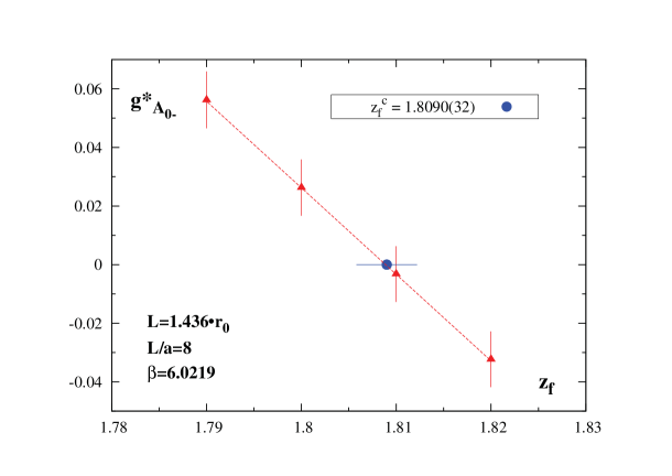
Figure 2: $g_{\mathrm{A}_{0-}}^{*}$ vs. $z_{f}$ (red). The fit is linear in $z_{f}$. The value of $z_{f}^{\rm cr}$, $z_{f}(g_{\mathrm{A}_{0-}}^{*}=0)$, is also plotted (blue).

All the numerical data for these intermediate steps can be found in ref. [33]. Next we determine $\kappa_{\rm cr}$.

• Using the same 16 pairs of $\kappa$ and $z_{f}$, we calculate $am_{\mathrm{PCAC}}$ as a function of $\kappa$ for each $z_{f}$. This is shown in fig. 3. Note that $am_{\mathrm{PCAC}}$ has a very mild dependence on $z_{f}$, so the four curves at fixed $z_{f}$ are nearly indistinguishable. Interpolating $am_{\mathrm{PCAC}}$ in $\kappa$ to the point of vanishing PCAC mass, $\kappa^{*}$, we obtain the values of $\kappa^{*}$ at each $z_{f}$. The resulting values of $\kappa^{*}$ as a function of $z_{f}$ are shown in fig. 4.

• We now interpolate these results in $z_{f}$ to the previously determined value of $z_{f}^{\rm cr}$, thus determining the value of $\kappa_{\rm cr}$.

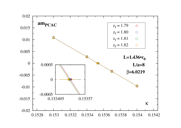
Figure 3: $am_{\mathrm{PCAC}}$ vs. $\kappa$ at four values of $z_{f}$ (open symbols). All fits are linear in $\kappa$. The values of $\kappa$ at $am_{\mathrm{PCAC}}=0$, denoted $\kappa^{*}$, are also plotted (filled symbols).

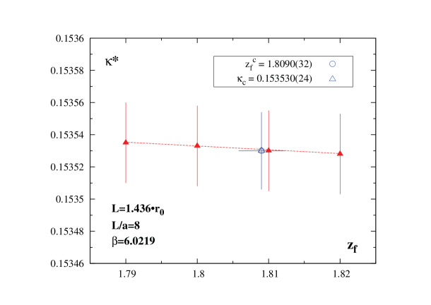
Figure 4: $\kappa^{*}$ vs. $z_{f}$ (red). The fit is linear in $z_{f}$. The value of $z_{f}^{\rm cr}$ (cf. fig. 2) and of $\kappa_{\rm cr}$, defined as $\kappa^{*}(z_{f}=z_{f}^{\rm cr})$, are also plotted (blue).

All the tuning results can be read off from tab. 8 and tab. LABEL:tab:zfc_beta.

A key observation of this work is the mild dependence of $am_{\mathrm{PCAC}}$ on $z_{f}$, at least in the region near $\kappa_{\rm cr}$ and $z_{f}^{\rm cr}$. This can be easily seen in fig. 3. The consequence of this is clear in fig. 4: the determination of $\kappa_{\rm cr}$ has a weak dependence on $z_{f}^{\rm cr}$ and the errors of both of them are relatively independent.

5.4 Tuning results

With the strategy discussed in sect. 5.3, we have performed the tuning of $\kappa$ and $z_{f}$ using $m_{\mathrm{PCAC}}$ in Eq. (5.12) and the conditions (1)-(7) defined in Eq. (5.13). The tuning has been performed for five fixed values of the renormalized gauge coupling, $\overline{g}(L)$, which correspond to five values of the physical energy scale, $1/L$. In particular, the physical scale ranges from the purely non-perturbative to the perturbative regime and 14 values of $\beta$ have been considered within that range. For better clarity, the tuning points are summarized in tab. 2. The notation in this table is the following. ‘Scale’ refers to the physical scale, namely, the fixed value of the renormalized gauge coupling. We have denoted the five scales as ‘NP’, ‘I’, ‘P’, ‘2P’ and ‘PP’, from the hadronic to the most perturbative scale. NP corresponds to $L=1.436\,r_{0}$, I to $\overline{g}^{2}=2.4484$ and P to $\overline{g}^{2}=0.9944$. For 2P and PP we have not determined the gauge coupling explicitly. These two scales have been considered in order to study the dependence of $z_{f}$ on $g_{0}$, for small values of $g_{0}$, thinking of a future perturbative determination of $z_{f}$, for which the knowledge of the renormalized coupling is not necessary. The results obtained for $\kappa_{\rm cr}$ and $z_{f}^{\rm cr}$ using the strategy outlined in sect. 5.3 for all the tuning methods are summarized in tab. 8 and tab. LABEL:tab:zfc_beta for $\kappa_{\rm cr}$ and $z_{f}^{\rm cr}$, respectively. We also present tables showing the values used for $z_{f}$ and $\kappa$, at each of the points where the tuning was performed. In these same tables, the column labelled ‘$N_{\textrm{conf}}$’ represents the number of configurations used in the computation of all observables at the corresponding point. These are tab. LABEL:tab:tuning_guess_np_new to tab. LABEL:tab:tuning_guess_pp_new.

Scale	$L/a$	$\beta$	Name
$L=1.436\,r_{0}$	8	6.0219	NP
	10	6.1628
	12	6.2885
	16	6.4956
	20	6.6790
	24	6.8187
$\overline{g}^{2}=2.4484$	8	7.0197	I
	12	7.3551
	16	7.6101
$\overline{g}^{2}=0.9944$	8	10.3000	P
	12	10.6086
	16	10.8910
	16	12.0000	2P
	16	24.0000	PP

Table 2: Summary of all the points where the tuning was performed.

During the tuning, we have used several combinations of $\kappa$ and $z_{f}$. As indicated in sect. 5.3, the usual choice is to use 4 values of $\kappa$ and 4 values of $z_{f}$. However, there are cases where we have used, instead, 5 values of $z_{f}$ and/or 2 values of $\kappa$. In particular, we have used 2 values of $\kappa$ at all the $\beta$ values where we also performed the separate tuning using (1*). The reason is that, relying on the very weak dependence of $\kappa$ and $z_{f}$ on each other, as it was shown in figs. 3 to 4, we expected the value of $\kappa_{\rm cr}$ not to change appreciably even if $z_{f}^{\rm cr}$ would vary visibly from one method to another. Therefore, we considered that the value of $\kappa_{\rm cr}$ obtained using (1*) was already a very accurate guess on where the critical value of $\kappa$ should be using all the other conditions. In fact, these expectations were later confirmed from our results of $\kappa_{\rm cr}$, which, from one method to another, are the same within statistical errors. Actually, in most cases $\kappa_{\rm cr}$ did not change in any digit between any of the methods employed in the determination of $z_{f}^{\rm cr}$ (cf. tab. 8).

On the contrary, changes in $z_{f}^{\rm cr}$ among the different methods are particularly manifest. This may be seen better in tab. LABEL:tab:zfc_beta. Here we can see how, in most cases, $z_{f}^{\rm cr}$ does not agree within errors from one method to another. This behavior becomes stronger at lower energies, i.e. for decreasing values of $\beta$. Even if $z_{f}^{\rm cr}$ does not agree from one method to another, the differences are expected to be only O($a$) discretization effects and, as such, should vanish in the continuum limit linearly in the lattice spacing.

In order to check this expectation, we have performed the continuum limit of differences in $z_{f}^{\rm cr}$, as determined from different methods, at the lowest value of the renormalization scale (cf. also [34]). In particular, the data correspond to the differences

$$\Delta z_{f}^{\rm cr}(m)=z_{f}^{\rm cr}(1)-z_{f}^{\rm cr}(m)\,,\quad m=2,3,4,5,6,7\,.$$ (5.14)

The data for $\Delta z_{f}^{\rm cr}(m)$ are presented in tab. LABEL:tab:Delta_zf_1M_np_cl for all the methods and the corresponding fits, linear in $a/L$, are given in tab. LABEL:tab:Fit_Delta_zf_1M_np_cl where the point $L/a=8$ has been excluded from all the fits. The data for $\Delta z_{f}^{\rm cr}(m)$, together with the extrapolation to the continuum limit are plotted in fig. 5. From this analysis we can conclude that the differences in $z_{f}^{\rm cr}$ from different methods are only cutoff effects of O($a$), as expected, which vanish in the continuum limit. This result may be considered as an additional test of the universality of the continuum limit. Moreover, discrepancies of O($a$) between different values of $z_{f}^{\rm cr}$ should affect physical observables at $O(a^{2})$ at most. This expectation will be confirmed in the following section, where we analyze the dependence of several quantities on the particular tuning condition.

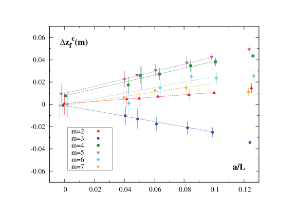
Figure 5: Differences of $z_{f}^{\rm cr}$, $\Delta z_{f}^{\rm cr}(m)$, as determined from different methods (cf. eq. (5.14)). The differences are always $z_{f}^{\rm cr}(1)$ minus $z_{f}^{\rm cr}(m)$, determined from any other method $m=2\dots 7$. The data are presented in tab. LABEL:tab:Delta_zf_1M_np_cl. All extrapolations to the continuum limit are linear in $a/L$ and the point $L/a=8$ is excluded from all the fits. The results from the fits are presented in tab. LABEL:tab:Fit_Delta_zf_1M_np_cl. The points from the different methods have been plotted slightly displaced from each other.

5.5 Conclusions on the tuning

We have presented the results of the non-perturbative tuning of $\kappa$ and $z_{f}$ for the $\chi$SF at several physical scales, for a range of lattice spacings, and using 7 different definitions of $z_{f}^{\rm cr}$. Our results demonstrate that the tuning of these two coefficients is indeed feasible, at least in the quenched approximation. Moreover, we observe that the tuning of $z_{f}$ and $\kappa$ are nearly independent. This observation is important, having in mind dynamical fermion simulations; if this behaviour persists with dynamical calculations, it may ease the numerical effort necessary to perform the tuning, thus reducing the number of required simulations. We have also shown that even if $z_{f}^{\rm cr}$ differs from one method to another at finite values of the cutoff, such differences are only O($a$) discretization effects, as expected theoretically. These discrepancies vanish in the continuum limit, which itself provides numerical evidence of the universality of the continuum limit.

6 Scaling studies and universality of the continuum limit

In the present section, we show the results of our scaling analysis of several correlation functions that have been computed using the values of the critical parameters, $\kappa_{\rm cr}$ and $z_{f}^{\rm cr}$, as determined from each of the 7 tuning conditions defined in sect. 5.2. We have carried out these studies at all the $\beta$ values at which the tuning has been performed. In sect. 5.4 we have shown that different definitions of $z_{f}^{\rm cr}$ lead to critical values of $z_{f}$ that differ from each other by cutoff effects of O($a$). With the scaling study presented here, we demonstrate that these discrepancies in $z_{f}^{\rm cr}$ do not influence the continuum limit value of physical observables. This is a very important result since the continuum limit must be independent of the particular definition of the critical parameters. Furthermore, we will show that physically relevant quantities, when determined from the different values of $z_{f}^{\rm cr}$, agree within statistical errors already at non-zero lattice spacing, even at the coarsest lattices. This agreement holds even at the matching scale with the hadronic scheme, where cutoff effects are expected to be largest. Indeed, the agreement at non-zero lattice spacing indicates that the discretization effects induced by the O($a$) uncertainties in $z_{f}^{\rm cr}$ are very small.

In order to analyze the different correlation functions, we have classified them in three types. The first, discussed in sect. 6.1, are those ${\mathcal{R}}_{5}^{1,2}$-even correlation functions that have a non-vanishing continuum limit, which we refer to as ’physical’. These are the only quantities which are expected to be automatic O($a$)-improved (up to boundary effects), provided $\kappa$ and $z_{f}$ are correctly tuned to their critical values. The second kind, detailed in sect. 6.2, are those ${\mathcal{R}}_{5}^{1,2}$-even correlation functions which vanish in the continuum limit, if the correct $\chi$SF b.c. (3.7) are recovered in the continuum limit. The last type, sect. 6.3, are ${\mathcal{R}}_{5}^{1,2}$-odd quantities. They should vanish in the continuum limit up to O($a$) cutoff effects if ${\mathcal{R}}_{5}^{1,2}$-symmetry is restored in the continuum limit.

These 3 kinds of correlation functions have been obtained from the definitions of the boundary to bulk correlation functions given in eq. (5.5). For unexplained notations in this section, the reader is referred to sect. 5.1. With suitable combinations of the Dirac and flavor indices in eq. (5.5), we can define correlation functions which are either even or odd under ${\mathcal{R}}_{5}^{1,2}$ transformations. All correlation functions labelled with $+$ should vanish in the continuum limit if the correct boundary conditions are recovered, independently of symmetry considerations. On the contrary, all those labelled with $-$ are a priori different from zero, unless some symmetry requires them to vanish.

Boundary to bulk correlation functions are normalized in a standard fashion with certain boundary to boundary correlation functions in order to cancel the renormalization of the boundary quark fields. In particular in this work, only one such boundary to boundary correlation function is considered. It is the equivalent of $f_{1}$ [38] in the standard SF and it is defined as,

$$g_{1}^{ab}(\theta)=-\frac{1}{L^{6}}\,\langle\widetilde{\mathcal{P}^{\prime}}_{+}^{a}\widetilde{\mathcal{P}}_{-}^{b}\rangle\,.$$ (6.1)

Note that the combination of signs in Eq. (6.1) is the only possibility for $g_{1}^{ab}$ not to vanish in the continuum limit, according to the boundary conditions satisfied in the continuum.

6.1 ${\mathcal{R}}_{5}^{1,2}$-even correlation functions

For 14 values of $\beta$ and several kinematic conditions, we have analyzed the ${\mathcal{R}}_{5}^{1,2}$-even correlation functions $g_{\mathrm{P}_{-}}^{11}$, $g_{\mathrm{V}_{0-}}^{12}$ and $g_{1}^{11}$ as defined in eq. (5.5) and in eq. (6.1). The correlation functions determined at the values of $\kappa_{\rm cr}$ and $z_{f}^{\rm cr}$ obtained from the tuning conditions (1) to (7) for all the $\beta$ values and all the renormalization scales considered are collected in tabs. LABEL:tab:ecf_0.0_newtun_np-LABEL:tab:ecf_0.5_newtun_pp. In tabs. LABEL:tab:ecf_0.0_newtun_np-LABEL:tab:ecf_0.0_newtun_pp we give results at $\boldsymbol{\theta}=(0,0,0)$, while in tabs. LABEL:tab:ecf_0.5_newtun_np-LABEL:tab:ecf_0.5_newtun_pp we collect results for $\boldsymbol{\theta}=(0.5,0.5,0.5)$.

The determination of all these quantities from the methods (1) to (7) has been performed via interpolations to $\kappa_{\rm cr}$ and $z_{f}^{\rm cr}$. To check that the interpolation does not introduce additional systematic errors, we have computed observables directly at $\kappa_{\rm cr}$ and $z_{f}^{\rm cr}$, without performing any interpolation from the first tuning method (cf. method (1*) in tabs. 8 and  LABEL:tab:zfc_beta). These data, computed at $\boldsymbol{\theta}=(0.5,0.5,0.5)$, are presented in tabs. LABEL:tab:ecf_0.5_newtun_np-LABEL:tab:ecf_0.5_newtun_p. We have checked for this particular tuning method that the quantities obtained via an interpolation of the data do agree within errors with those obtained by means of new computations performed directly at the critical values of $\kappa$ and $z_{f}$, denoted as method (1*). We therefore believe that the interpolation that we perform here does not induce additional errors.

From this analysis we have found that for all the 14 values of $\beta$, all ${\mathcal{R}}_{5}^{1,2}$-even quantities with a non-vanishing continuum limit do not depend on the definition of $z_{f}^{\rm cr}$ within statistical errors. This holds for any of the values of the kinematical parameters that we have investigated. In fig. 6 we show, as an example, the dependence on the tuning conditions for $g_{\mathrm{P}_{-}}^{11}$ at the matching scale, $L=1.436\,r_{0}$, and for $\boldsymbol{\theta}=(0,0,0)$. Similar results are obtained for the other correlation functions.

The independence at each value of the lattice spacing on the tuning conditions, i.e. on the particular definition of $z_{f}^{\rm cr}$ adopted is reassuring: no large cutoff effects are introduced depending on the choice of the tuning condition. The continuum limit of renormalized quantities and their dependence on the tuning conditions will be discussed in the companion paper [18].

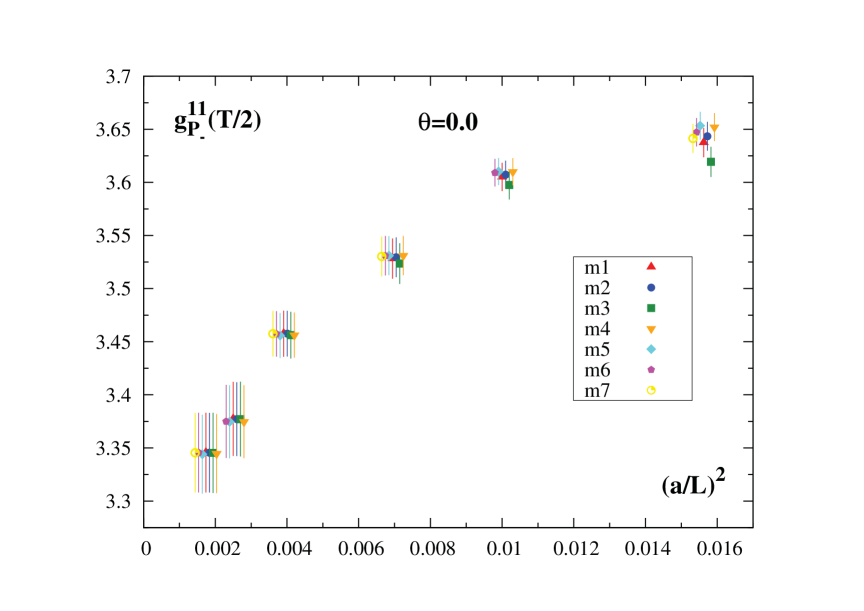
Figure 6: Comparison between different tuning conditions using the ${\mathcal{R}}_{5}^{1,2}$-even quantity $g_{\mathrm{P}_{-}}^{11}$. The scale is NP and $\boldsymbol{\theta}=(0,0,0)$. Data for all methods (1) to (7) are presented (cf. tab. LABEL:tab:ecf_0.0_newtun_np). No continuum limit is performed, since this quantity takes a finite value in the continuum limit only after renormalization. The purpose of the plot is to compare the results from the different tuning conditions at non-zero lattice spacing and a full agreement can be seen. The data from the different methods have been plotted slightly displaced from each other.

6.2 Recovery of the $\chi$SF boundary conditions

We present here results for the ${\mathcal{R}}_{5}^{1,2}$-even correlation functions which should vanish in the continuum limit, due to the particular form of the $\chi$SF boundary conditions in eqs. (3.7, 3.8) satisfied by the fermion fields in the continuum limit. We collect our results for the $g_{\mathrm{P}_{+}}^{11}$ and $g_{\mathrm{V}_{0+}}^{12}$ correlation functions at all the $\beta$ values and all the renormalization conditions in tabs. LABEL:tab:ecf_0.0_newtun_np-LABEL:tab:ecf_0.5_newtun_pp. We provide results for $\boldsymbol{\theta}=(0,0,0)$ in tabs. LABEL:tab:ecf_0.0_newtun_np-LABEL:tab:ecf_0.0_newtun_pp and for $\boldsymbol{\theta}=(0.5,0.5,0.5)$ in tabs. LABEL:tab:ecf_0.5_newtun_np-LABEL:tab:ecf_0.5_newtun_pp.

We found that for all the tuning conditions $g_{\mathrm{P}_{+}}^{11}$ and $g_{\mathrm{V}_{0+}}^{12}$ vanish in the continuum limit, signalling that the proper $\chi$SF b.c. are recovered. We have observed that the values of $g_{\mathrm{P}_{+}}^{11}$ and $g_{\mathrm{V}_{0+}}^{12}$ would change substantially if we vary the values of $z_{f}^{\rm cr}$ within their statistical errors. If we want to perform the continuum limit at fixed “physical” scale we have to take this variation into account. We do this by propagating the statistical error of $z_{f}^{\rm cr}$ when interpolating $g_{\mathrm{P}_{+}}^{11}$ and $g_{\mathrm{V}_{0+}}^{12}$ in $z_{f}$. We note that $g_{\mathrm{P}_{+}}^{11}$ and $g_{\mathrm{V}_{0+}}^{12}$ do not show the same behaviour for variations of $\kappa_{\rm cr}$.

We show in fig. 7 the behaviour of $g_{\mathrm{P}_{+}}^{11}(\boldsymbol{\theta=\boldsymbol{0}})$ towards the continuum limit. This is an example of a quantity that should vanish in the continuum limit if the proper b.c. conditions are recovered. Similar plots can be obtained for other quantities looking at the data in tabs. LABEL:tab:ecf_0.0_newtun_np-LABEL:tab:ecf_0.5_newtun_pp where the first error is statistical while the second, where available, contains the propagation of the error of $z_{f}^{\rm cr}$. As discussed in the previous and in the next section, we stress that this is the only case where we have observed that the statistical error of $z_{f}^{\rm cr}$ shows significant effects in the correlation functions.

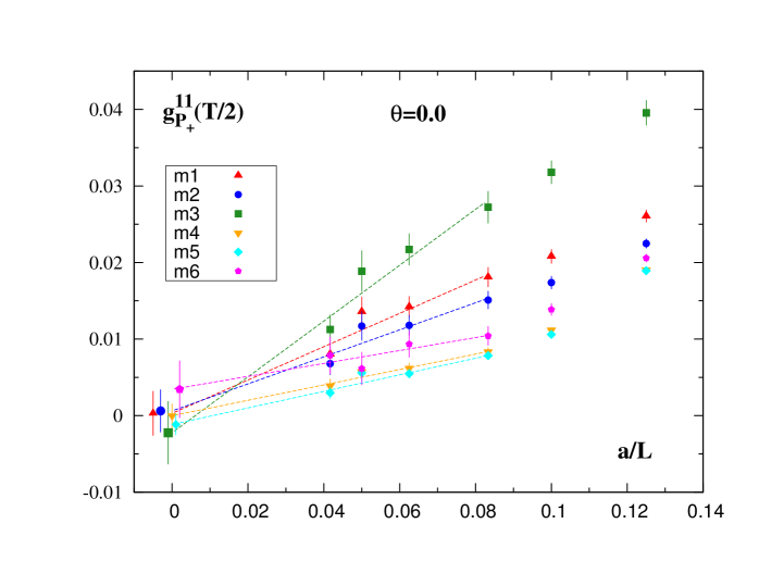
Figure 7: Approach to the continuum limit of the ${\mathcal{R}}_{5}^{1,2}$-even quantity $g_{\mathrm{P}_{+}}^{11}$. The scale is NP and $\boldsymbol{\theta}=(0,0,0)$. Data for methods (1) to (6) are presented (cf. tab. LABEL:tab:ecf_0.0_newtun_np). $g_{\mathrm{P}_{+}}^{11}$ is plotted here as a function of $a/L$. The error bars contain the statistical errors of the correlation functions together with the propagation of the statistical error on $z_{f}^{\rm cr}$.

6.3 ${\mathcal{R}}_{5}^{1,2}$-odd correlation functions

Amongst all the ${\mathcal{R}}_{5}^{1,2}$-odd correlation functions, we consider correlation functions that vanish only because of symmetry considerations, i.e. we do not consider correlation functions vanishing in the continuum limit because of the recovery of the $\chi$SF boundary conditions. Examples of such correlation functions are $g_{\mathrm{A}_{0-}}^{11}$ and $\overline{g}_{\mathrm{V}_{k-}}^{12}$. It is important to note that the same correlation functions have been used in the determination of $z_{f}^{\rm cr}$. When studying the dependence on the tuning condition towards the continuum limit of a given correlation function we have obviously excluded the value of $z_{f}^{\rm cr}$ obtained imposing that the same correlation function vanishes at each value of the lattice spacing. We have though studied the dependence of all the other tuning conditions towards the continuum limit.

The numerical results obtained at $\boldsymbol{\theta}=(0,0,0)$ are presented in tabs. LABEL:tab:ocf_0.0_newtun_np-LABEL:tab:ocf_0.0_newtun_pp, and the results for $\boldsymbol{\theta}=(0.5,0.5,0.5)$ are given in tabs. LABEL:tab:ocf_0.5_newtun_np-LABEL:tab:ocf_0.5_newtun_pp.

Although results from different definitions of $z_{f}^{\rm cr}$ do not coincide at non-zero lattice spacing, all the ${\mathcal{R}}_{5}^{1,2}$-odd correlation functions vanish in the continuum limit independently of the tuning condition adopted. This is strong evidence that ${\mathcal{R}}_{5}^{1,2}$-symmetry is restored in the continuum limit.

As an example we show in the plot of fig. 8 the continuum limit approach for $g_{\mathrm{A}_{0-}}^{11}$ with $\boldsymbol{\theta}=(0,0,0)$ and in the plot of fig. 9 the continuum limit of $\overline{g}_{\mathrm{V}_{k-}}^{12}$ for $\boldsymbol{\theta}=(0.5,0.5,0.5)$. These plots correspond to our most non-perturbative point, $L=1.436\,r_{0}$, which is the case where the cutoff effects are expected to be stronger. The data show a linear behaviour in $a/L$ and they have been fitted with a linear fit in $a/L$,

$$f=b_{0}+b_{1}\Big{(}\frac{a}{L}\Big{)}\,.$$ (6.2)

We have not considered the point $L/a=8$ in the fits. The results from the fits are summarized in tab. LABEL:tab:ga0_cl_np_fit for $g_{\mathrm{A}_{0-}}^{11}$ and in tab. LABEL:tab:gak_cl_np_fit for $\overline{g}_{\mathrm{V}_{k-}}^{12}$. As anticipated all the ${\mathcal{R}}_{5}^{1,2}$-odd correlation functions vanish within errors in the continuum limit. Not being automatic O($a$) improved they scale linearly in $a/L$ independently of the tuning condition adopted.

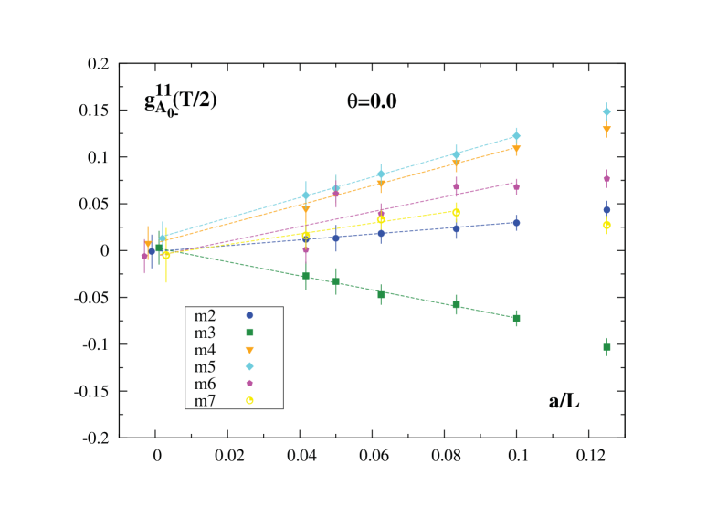
Figure 8: Extrapolation to the continuum limit of the ${\mathcal{R}}_{5}^{1,2}$-odd quantity $g_{\mathrm{A}_{0-}}^{11}$. The scale is NP and $\boldsymbol{\theta}=(0,0,0)$. Data for methods (2) to (7) are presented (cf. tab. LABEL:tab:ocf_0.0_newtun_np). The fits are all linear in $a/L$ (cf. tab. LABEL:tab:ga0_cl_np_fit). The point $L/a=8$ has been excluded from all the fits. We show the data for all tuning conditions except condition (1) because it corresponds to imposing $g_{\mathrm{A}_{0-}}^{11}=0$. The (vanishing) continuum limit values obtained from the different tuning conditions have been plotted slightly displaced from each other.

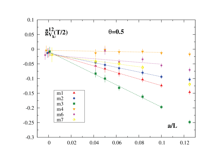
Figure 9: Extrapolation to the continuum limit of the ${\mathcal{R}}_{5}^{1,2}$-odd quantity $\overline{g}_{\mathrm{V}_{k-}}^{12}$. The scale is NP and $\boldsymbol{\theta}=(0.5,0.5,0.5)$. Data for methods (1) to (4) and (6) to (7) are presented (cf. tab. LABEL:tab:ocf_0.5_newtun_np). The fits are all linear in $a/L$ (cf. tab. LABEL:tab:gak_cl_np_fit). The point $L/a=8$ has been excluded from all the fits. We show the data for all tuning conditions except condition (5) because it corresponds to imposing $\overline{g}_{\mathrm{V}_{k-}}^{12}=0$.

6.4 Conclusions on the scaling analysis

From the analysis performed at several $\beta$ values at fixed renormalization scale, we learned that all quantities that should vanish in the continuum limit, either by boundary conditions or symmetry restoration, have a visible dependence on the tuning condition and the corresponding values of $z_{f}^{\rm cr}$.

The ${\mathcal{R}}_{5}^{1,2}$-even correlation functions that should vanish in the continuum limit, if the correct boundary conditions are recovered, show the strongest dependence on the way $z_{f}^{\rm cr}$ has been determined. In particular we have observed that to properly study the continuum limit we cannot simply take the central vale of $z_{f}^{\rm cr}$, but we need to propagate the statistical error of $z_{f}^{\rm cr}$ into the error for the correlation functions, i.e. the statistical fluctuations in $z_{f}^{\rm cr}$ are visible in the final values for the correlation functions. If one takes the statistical error of $z_{f}^{\rm cr}$ into account in the determination of the error of the correlation functions, we observe, for all the tuning conditions, that the proper boundary conditions are recovered in the continuum limit within errors. Additionally this result is confirmed for all the tuning conditions adopted.

This observation is in stark contrast with the ${\mathcal{R}}_{5}^{1,2}$-even correlation functions containing the non-vanishing component of the boundary fermion fields. In this case not only the statistical error on $z_{f}^{\rm cr}$ is irrelevant, but even the choice of the tuning condition for all practical purposes does not change the final values for the correlation functions even at non-zero lattice spacings. Although we can not make a general statement about all possible physical observables, our expectation is that other physical quantities, different from the ones studied in this work, will behave in the same manner. This is reassuring for further uses of the $\chi$SF for physical applications with dynamical fermions.

In the case of the ${\mathcal{R}}_{5}^{1,2}$-odd orrelation functions, we have shown that they vanish in the continuum limit with leading O($a$) discretization effects for all the tuning conditions, as expected. This is strong numerical evidence of the restoration of ${\mathcal{R}}_{5}^{1,2}$-symmetry in the continuum limit and the independence of the continuum limit on the particular tuning condition. This result is also an indication that the correct boundary conditions are recovered in the continuum limit.

7 Conclusions

Large scale simulations with Wilson twisted mass fermions at maximal twist need a renormalization scheme that preserves the property of automatic O($a$) improvement. The RI-MOM scheme is consistent with this requirement and results for $N_{f}=2$ dynamical fermions have been obtained in ref. [39] and preliminary $N_{f}=4$ results have been presented in ref. [40]. Recently the x-space scheme has been tested on the $N_{f}=2$ twisted mass ensembles [41]. One of the problems with these schemes is that it is difficult to cover the large range of scales necessary to bridge the perturbative and non-perturbative regimes.

Finite volume schemes have been developed to tackle this problem. These schemes can be used to perform the continuum limit of step-scaling functions and to carry out the non-perturbative renormalization, especially for scale-dependent quantities. Thus it is very desirable to have the possibility to use finite volume renormalization schemes together with Wilson twisted mass fermions. In this work we have made a detailed study of the $\chi$SF scheme proposed in ref. [16] with quenched Wilson fermions. Bulk automatic O($a$) improvement is achieved with a single non-perturbative tuning of the parameter $z_{f}$ to its critical value $z_{f}^{\rm cr}$, together with the usual tuning of $\kappa_{\rm cr}$. We have proposed a tuning strategy for the simultaneous determination of $z_{f}^{\rm cr}$ and $\kappa_{\rm cr}$ and we have perfomed a feasibility study of several tuning conditions, showing that the tuning is affordable with the current computer resources and it does not pose any specific problem.

The study presented in this work has shown that, as expected, unphysical correlation functions vanish in the continuum limit with O($a$) corrections independently of the tuning condition adopted and that the proper boundary conditions are recovered in the continuum limit. In addition physical correlation functions are rather insensitive to the method employed to determine $\kappa_{\rm cr}$ and $z_{f}^{\rm cr}$. This is a very promising result since it will ease the computational effort required to go beyond the quenched approximation.

In a companion paper [18] we will further investigate the continuum limit scaling behaviour of physical quantities that are renormalized through the $\chi$SF scheme employing the results of $\kappa_{\rm cr}$ and $z_{f}^{\rm cr}$ determined in this work.

Appendix A Symmetries in the twisted basis

We list in this appendix the form of a few symmetry tranfosrmations in the twisted basis. The twisted basis $\{\chi\,,\overline{\chi}\}$ and the standard basis $\{\psi\,,\overline{\psi}\}$ are related by the non-anomalous axial transformation

$$\psi(x)=\exp\left(i\,\frac{\omega}{2}\,\gamma_{5}\,\tau^{3}\right)\,\chi(x)\,,\qquad\overline{\psi}(x)=\overline{\chi}(x)\,\exp\left(i\,\frac{\omega}{2}\,\gamma_{5}\,\tau^{3}\right)\,.$$ (A.1)

Charge conjugation $\mathcal{C}$ is invariant under this basis transformation

$$\mathcal{C}\colon\begin{cases}U(x;\mu)\rightarrow U(x;\mu)^{*},\\ \chi(x)\rightarrow C^{-1}\overline{\chi}(x)^{T},\\ \overline{\chi}(x)\rightarrow-\chi(x)^{T}C,\end{cases}$$ (A.2)

where $C$ satisfies

$$-\gamma_{\mu}^{T}=C\gamma_{\mu}C^{-1},\qquad\gamma_{5}=C\gamma_{5}C^{-1}.$$ (A.3)

Parity and time reversal are affected by the rotation and take a different form in the twisted basis. In this basis they are denoted $\mathcal{P}_{\omega}$ and $\mathcal{T}_{\omega}$, respectively, and have the expressions

$$\mathcal{P}_{\omega}\,:\,\begin{cases}U_{0}(x_{0},\vec{x})\,\rightarrow\,U_{0}(x_{0},-\vec{x})\,,\quad U_{k}(x_{0},\vec{x})\,\rightarrow\,U_{k}^{\dagger}(x_{0},-\vec{x}-\vec{k})\\ \chi(x_{0},\vec{x})\,\rightarrow\,\gamma_{0}\,\exp\left(i\,\omega\,\gamma_{5}\,\tau^{3}\right)\,\chi(x_{0},-\vec{x})\\ \overline{\chi}(x_{0},\vec{x})\,\rightarrow\,\overline{\chi}(x_{0},-\vec{x})\,\exp\left(i\,\omega\,\gamma_{5}\,\tau^{3}\right)\,\gamma_{0}\end{cases}$$ (A.4)

$$\mathcal{T}_{\omega}\,:\,\begin{cases}U_{0}(x_{0},\vec{x})\,\rightarrow\,U_{0}^{\dagger}(-x_{0}-a,\vec{x})\,,\quad U_{k}(x_{0},\vec{x})\,\rightarrow\,U_{k}(-x_{0},\vec{x})\\ \chi(x_{0},\vec{x})\,\rightarrow\,i\,\gamma_{0}\,\gamma_{5}\,\exp\left(i\,\omega\,\gamma_{5}\,\tau^{3}\right)\,\chi(-x_{0},\vec{x})\\ \overline{\chi}(x_{0},\vec{x})\,\rightarrow\,\overline{\chi}(-x_{0},\vec{x})\,\exp\left(i\,\omega\,\gamma_{5}\,\tau^{3}\right)\,i\,\gamma_{0}\,\gamma_{5}\,.\end{cases}$$ (A.5)

To obtain the form of a parity or a time-reversal transformation in the standard basis, $\mathcal{P}$ or $\mathcal{T}$, it is sufficient to set $\omega=0$ in eqs (A.4) and (A.5).

In the twisted basis the $SU(2)$ vector transformation takes the form

$$SU(2)_{\omega}\colon\begin{cases}\chi(x)\rightarrow\exp\left(-i\,\frac{\omega}{2}\,\gamma_{5}\,\tau^{3}\right)\,\exp\left(i\,\frac{\alpha_{V}^{a}}{2}\,\tau^{a}\right)\,\exp\left(i\,\frac{\omega}{2}\,\gamma_{5}\,\tau^{3}\right)\,\chi(x),\\ \overline{\chi}(x)\rightarrow\overline{\chi}(x)\,\exp\left(i\,\frac{\omega}{2}\,\gamma_{5}\,\tau^{3}\right)\,\exp\left(-i\,\frac{\alpha_{V}^{a}}{2}\,\tau^{a}\right)\,\exp\left(-i\,\frac{\omega}{2}\,\gamma_{5}\,\tau^{3}\right).\end{cases}$$ (A.6)

Appendix B The free lattice quark propagator for the $\chi$SF with Wilson fermions

In this appendix we obtain the analytical expression of the quark propagator $S\left(x,y\right)$ on the lattice at tree-level of perturbation theory for the action in eq. (4.1). The derivation of the propagator is rather standard (see for example ref. [42]) once we have the exact b.c. satisfied by the fermion fields at finite lattice spacing $a$. They can be obtained as a spinoff of the orbifold construnctions [16] and read

$$\widetilde{Q}_{+}\left(1-\frac{a}{2}\partial^{*}_{0}\right)S(x,y)|_{x_{0}=0}=0\qquad\widetilde{Q}_{-}\left(1+\frac{a}{2}\partial_{0}\right)S(x,y)|_{x_{0}=T}=0\,.$$ (B.1)

The problem we want to solve is then

$$\left(D_{\textrm{W}}+m_{0}\right)\,S\left(x,y\right)=a^{-4}\,$$ (B.2)

with b.c. (B.1) where $\delta_{x,y}$ is the dimensionless Kronecker delta and $D_{W}$ denotes the massless Wilson operator (4.4).

The result of the calculation can be cast in the form

$$S\left(x,y\right)=\left(D_{\textrm{W}}^{\dagger}+m_{0}\right)\,G\left(x,y\right)\,,$$ (B.3)

with

$$G\left(x,y\right)=\frac{1}{L^{3}}\,\sum_{\vec{p}}\,e^{i\vec{p}\left(\vec{x}-\vec{y}\right)}\,G\left(x_{0},y_{0};\vec{p}\right)\,,$$ (B.4)

where

$$\begin{split}G\left(x_{0},y_{0};\vec{p}\right)=\frac{1}{2\mathaccent 23{\omega}(\vec{p}^{+})A(\vec{p}^{+})D(p^{+})}&\Big{\{}\,\>e^{-\omega(\vec{p}^{+})|x_{0}-y_{0}|}-e^{-\omega(\vec{p}^{+})\left(2\left(T+a\right)-|x_{0}-y_{0}|\right)}\\ &-i\gamma_{0}\gamma_{5}\tau^{3}e^{-\omega(\vec{p}^{+})\left(x_{0}+y_{0}+a\right)}\\ &+i\gamma_{0}\gamma_{5}\tau^{3}e^{-\omega(\vec{p}^{+})\left(2\left(T+a\right)-\left(x_{0}+y_{0}+a\right)\right)}\>\Big{\}}\,.\end{split}$$ (B.5)

Here we list all the definitions of the functions useful for the determination of the propagator.

$$p_{\mu}^{\pm}=p_{\mu}\pm\theta_{\mu}/L\,,\qquad\theta_{0}=0\,,$$ (B.6)

$$\hbox{\accent 23{$\!\!\!\! p$}}_{\mu}^{\pm}=\frac{1}{a}\sin\left(ap_{\mu}^{\pm}\right)\,,\qquad\mathcal{M}(p^{\pm})=m_{0}+\frac{1}{2}a\hat{p}^{\pm\,2}_{\mu}\,,\qquad\hat{p}_{\mu}^{\pm}=\frac{2}{a}\sin\left(\frac{ap_{\mu}^{\pm}}{2}\right)\,.$$ (B.7)

The function $\omega(\vec{p}^{+})$, such that $p_{0}=i\omega(\vec{p}^{+})$, is given by

$$\sinh\left[\frac{a}{2}\omega\left(\vec{p}^{\pm}\right)\right]=\left\{\frac{a^{2}\hbox{\accent 23{$\!\!\!\! p$}}^{\pm\,2}_{k}+\left(A(\vec{p}^{\pm})-1\right)^{2}}{4A(\vec{p}^{\pm})}\right\}^{1/2}\,,$$ (B.8)

and

$$\mathaccent 23{\omega}(p^{\pm})\equiv-i\hbox{\accent 23{$\!\!\!\! p$}}_{0}^{\pm}=\frac{1}{a}\,\sinh\left[a\omega(\vec{p}^{\pm})\right]\,,$$ (B.9)

$$A\left(\vec{p}^{\pm}\right)\equiv 1+a\left(m_{0}+\frac{a}{2}\hat{p}_{k}^{\pm\,2}\right)\,,$$ (B.10)

$$D(p^{\pm})\equiv 1+e^{-2\omega(\vec{p}^{\pm})\left(T+a\right)}\,.$$ (B.11)

The analytical expression of the lattice quark propagator (B.3) has been numerically cross-checked with the propagator obtained from a numerical inversion of the free lattice Dirac operator given in Eq. (4.2) and also with the corresponding propagator in [16].

Appendix C Tables of numerical results

C.1 Tuning data

Table 3: Values of $\kappa$ and $z_{f}$ used for the tuning and number of configurations, $N_{\textrm{conf}}$, used in all calculations at the corresponding value of $\beta$. Scale NP (see text). The data of the last three columns have been used only for a separate analysis with method (1), which we denote here as method (1*).

Guess values for the tuning
Hadronic scale: $L=1.436\,r_{0}$
$L/a$	$\beta$	$N_{\textrm{conf}}$	$z_{f}$	$\kappa$	$N_{\textrm{conf}}$	$z_{f}$	$\kappa$
8	6.0219	1000	1.74	0.1534	1000	1.79	0.1530
			1.77	0.1537		1.80	0.1534
			1.80			1.81	0.1537
			1.83			1.82	0.1540
			1.86
10	6.1628	1000	1.73	0.1521	1000	1.78	0.1520
			1.76	0.1522		1.79	0.1521
			1.79			1.80	0.1522
			1.82			1.81	0.1523
12	6.2885	500	1.71	0.15050	300	1.70	0.15025
			1.74	0.15100		1.73	0.15050
			1.77			1.77	0.15100
			1.80			1.80	0.15125
16	6.4956	300	1.64	0.1489	100	1.70	0.1488
			1.67	0.1490		1.71	0.1489
			1.70			1.73	0.1490
			1.73			1.74	0.1491
			1.76
20	6.6790	112	1.66	0.1473
			1.68	0.1474
			1.70	0.1475
			1.72	0.1476
24	6.8187	100	1.60	0.1463
			1.63	0.1464
			1.66	0.1465
			1.69	0.1466

Table 4: Same caption as in tab. LABEL:tab:tuning_guess_np_new but at scale I (see text).

Guess values for the tuning
Intermediate scale: $\overline{g}^{2}=2.4484$
$L/a$	$\beta$	$N_{\textrm{conf}}$	$z_{f}$	$\kappa$	$N_{\textrm{conf}}$	$z_{f}$	$\kappa$
8	7.0197	1000	1.51	0.14445	1000	1.35	0.14440
			1.54	0.14450		1.45	0.14445
			1.57			1.55	0.14450
			1.60			1.65	0.14455
12	7.3551	500	1.46	0.1431	300	1.50	0.1430
			1.49	0.1432		1.51	0.1431
			1.52			1.52	0.1432
			1.55			1.53	0.1433
16	7.6101	300	1.44	0.1421	100	1.48	0.1420
			1.47	0.1422		1.49	0.1421
			1.50			1.50	0.1422
			1.53			1.51	0.1423

Table 5: Same caption as in tab. LABEL:tab:tuning_guess_np_new but at scale P (see text).

Guess values for the tuning
Perturbative scale: $\overline{g}^{2}=0.9944$
$L/a$	$\beta$	$N_{\textrm{conf}}$	$z_{f}$	$\kappa$	$N_{\textrm{conf}}$	$z_{f}$	$\kappa$
8	10.3000				1000	1.2955	0.13541
						1.2965	0.13544
						1.2975	0.13547
						1.2985	0.13550
12	10.6086				300	1.292	0.13514
						1.294	0.13517
						1.297	0.13520
						1.299	0.13523
16	10.8910	300	1.23	0.13484	100	1.285	0.13482
			1.26	0.13487		1.286	0.13484
			1.29			1.287	0.13487
			1.32			1.288	0.13489

Table 6: Same caption as in tab. LABEL:tab:tuning_guess_np_new but at scale 2P (see text). Here no separate tuning was performed for method (1).

Guess values for the tuning
2P scale
$L/a$	$\beta$	$N_{\textrm{conf}}$	$z_{f}$	$\kappa$
16	12.0000	100	1.23	0.1335
			1.24	0.1336
			1.25	0.1337
			1.26	0.1338

Table 7: Same caption as in tab. LABEL:tab:tuning_guess_np_new but at scale PP (see text). Here no separate tuning was performed for method (1).

Guess values for the tuning
PP scale
$L/a$	$\beta$	$N_{\textrm{conf}}$	$z_{f}$	$\kappa$
16	24.0000	80	1.11	0.1287
			1.12	0.1288
			1.13	0.1289
			1.14	0.1290

C.2 Tuning results

$\beta$	$\kappa_{\rm cr}(1^{*})$	$\kappa_{\rm cr}(1)$	$\kappa_{\rm cr}(2)$	$\kappa_{\rm cr}(3)$	$\kappa_{\rm cr}(4)$	$\kappa_{\rm cr}(5)$	$\kappa_{\rm cr}(6)$	$\kappa_{\rm cr}(7)$	$\kappa_{\rm cr}(SF)$
Hadronic scale: $L=1.436\,r_{0}$ ($\mu\sim 300\mathrm{MeV}$)
6.0219	0.153530 (24)	0.15353 (66)	0.15354 (66)	0.15352 (67)	0.15354 (66)	0.15354 (66)	0.15354 (66)	0.15353 (66)	0.153371 (10)
6.1628	0.152134 (17)	0.15213 (66)	0.15214 (66)	0.15213 (67)	0.15214 (66)	0.15214 (66)	0.15214 (66)		0.152012 (7)
6.2885	0.150815 (22)	0.15082 (66)	0.15082 (66)	0.15082 (66)	0.15082 (65)	0.15082 (65)	0.15082 (65)	0.15082 (66)	0.150752 (10)
6.4956	0.148945 (25)	0.14894 (34)	0.14894 (33)	0.14893 (34)	0.14894 (33)	0.14894 (33)	0.14894 (33)	0.14894 (33)	0.148876 (13)
6.6790		0.14748 (74)	0.14748 (74)	0.14748 (74)	0.14748 (73)	0.14748 (73)	0.14748 (73)
6.8187		0.14645 (41)	0.14645 (41)	0.14645 (42)	0.14645 (41)	0.14645 (41)	0.14645 (41)	0.14645 (41)
Intermediate scale: $\overline{g}^{2}=2.4484$ ($\mu\sim 1\mathrm{GeV}$)
7.0197	0.144501 (13)	0.14450 (41)	0.14450 (41)	0.14450 (41)	0.14450 (41)	0.14450 (41)	0.14450 (41)	0.14450 (41)	0.144454 (7)
7.3551	0.143113 (12)	0.14311 (29)	0.14311 (29)	0.14311 (29)	0.14311 (29)	0.14311 (29)	0.14311 (29)	0.14311 (29)	0.143113 (6)
7.6101	0.142112 (13)	0.14212 (23)	0.14212 (23)	0.14212 (23)	0.14212 (23)	0.14212 (23)	0.14212 (23)	0.14212 (23)	0.142107 (6)
Perturbative scale: $\overline{g}^{2}=0.9944$ ($\mu\sim 30\mathrm{GeV}$)
10.3000	0.1354609 (54)								0.135457 (5)
10.6086	0.1351758 (56)								0.135160 (4)
10.8910	0.1348440 (61)	0.134844 (93)	0.134844 (93)	0.134844 (93)	0.134844 (93)	0.134844 (93)	0.134844 (93)	0.134844 (93)	0.134849 (6)
2P scale
12.0000		0.13363 (41)	0.13363 (41)	0.13363 (41)	0.13363 (41)	0.13363 (41)	0.13363 (41)	0.13363 (41)
PP scale
24.0000		0.12877 (15)	0.12877 (15)	0.12877 (15)	0.12877 (15)	0.12877 (15)	0.12877 (15)	0.12877 (15)

Table 8: Summary table of $\kappa_{\rm cr}$ for all beta values and tuning conditions, (1) to (7) (see sect. 5.2 for a description of all the methods). The data of column (1*) correspond to a separate analysis with method (1), using slightly different simulation parameters (cf. tab. LABEL:tab:tuning_guess_np_new, tab. LABEL:tab:tuning_guess_int_new and tab. LABEL:tab:tuning_guess_p_new). For reference, we also give $\kappa_{\rm cr}$ for the SF [43, 6, 44].

Table 9: Summary table of $z_{f}^{\rm cr}$ for all beta values and tuning conditions, (1) to (7) (see sect. 5.2 for a description of all the methods). The data of column (1*) correspond to a separate analysis with method (1), using slightly different simulation parameters (cf. tab. LABEL:tab:tuning_guess_np_new, tab. LABEL:tab:tuning_guess_int_new and tab. LABEL:tab:tuning_guess_p_new).

$\beta$	$z_{f}^{\rm cr}(1^{*})$	$z_{f}^{\rm cr}(1)$	$z_{f}^{\rm cr}(2)$	$z_{f}^{\rm cr}(3)$	$z_{f}^{\rm cr}(4)$	$z_{f}^{\rm cr}(5)$	$z_{f}^{\rm cr}(6)$	$z_{f}^{\rm cr}(7)$
Hadronic scale: $L=1.436\,r_{0}$
6.0219	1.8090 (32)	1.8091 (32)	1.7946 (34)	1.8434 (37)	1.7656 (27)	1.7597 (27)	1.7835 (40)	1.7980 (17)
6.1628	1.7920 (30)	1.7923 (29)	1.7820 (31)	1.8175 (33)	1.7541 (25)	1.7497 (25)	1.7687 (38)
6.2885	1.7664 (51)	1.7658 (38)	1.7573 (40)	1.7869 (46)	1.7312 (34)	1.7283 (32)	1.7408 (56)	1.7509 (22)
6.4956	1.7212 (83)	1.7201 (41)	1.7132 (44)	1.7377 (46)	1.6929 (35)	1.6894 (34)	1.7053 (63)	1.7076 (21)
6.6790		1.6841 (56)	1.6789 (59)	1.6973 (65)	1.6582 (52)	1.6577 (52)	1.6600 (90)
6.8187		1.6427 (56)	1.6381 (60)	1.6529 (60)	1.6253 (51)	1.6201 (50)	1.6421 (88)	1.6366 (27)
Intermediate scale: $\overline{g}^{2}=2.4484$
7.0197	1.5467 (15)	1.5404 (16)	1.5296 (17)	1.5597 (18)	1.5156 (14)	1.5126 (14)	1.5229 (21)	1.5392 (12)
7.3551	1.5126 (23)	1.5139 (18)	1.5088 (19)	1.5233 (19)	1.4955 (16)	1.4945 (15)	1.4981 (23)	1.5120 (12)
7.6101	1.4942 (37)	1.4943 (20)	1.4908 (21)	1.5007 (23)	1.4800 (18)	1.4789 (17)	1.4827 (28)	1.4916 (13)
Perturbative scale: $\overline{g}^{2}=0.9944$
10.3000	1.29730 (67)
10.6086	1.2954 (11)
10.8910	1.2858 (15)	1.28692 (88)	1.28487 (91)	1.28984 (99)	1.27999 (83)	1.27976 (75)	1.2805  (13)	1.28619 (67)
2P scale
12.0000		1.2493 (14)	1.2481 (14)	1.2510 (15)	1.2438 (13)	1.2443 (12)	1.2428 (20)	1.2494 (10)
PP scale
24.0000		1.11268 (57)	1.11162 (58)	1.11391 (65)	1.11013 (54)	1.11003 (48)	1.11030 (87)	1.11269 (50)

Table 10: Differences of $z_{f}^{\rm cr}$, $\Delta z_{f}^{\rm cr}(m)$, determined from different methods. The differences are always $z_{f}^{\rm cr}(1)$ minus $z_{f}^{\rm cr}(m)$, obtained from any other method $m=2\dots 7$. Scale NP.

$\Delta z_{f}^{\rm cr}(m)$ for different methods
Hadronic scale: $L=1.436\,r_{0}$
$L/a$	2	3	4	5	6	7
8	0.0145 (47)	-0.0343 (49)	0.0435 (42)	0.0494 (42)	0.0256 (51)	0.0111 (36)
10	0.0103 (42)	-0.0252 (44)	0.0382 (38)	0.0426 (38)	0.0236 (48)
12	0.0085 (55)	-0.0211 (60)	0.0346 (51)	0.0375 (50)	0.0250 (68)	0.0149 (44)
16	0.0069 (60)	-0.0176 (62)	0.0272 (54)	0.0307 (53)	0.0148 (75)	0.0125 (46)
20	0.0052 (81)	-0.0132 (86)	0.0259 (76)	0.0264 (76)	0.024 (11)
24	0.0046 (82)	-0.0102 (82)	0.0174 (76)	0.0226 (75)	0.001 (10)	0.0061 (62)

Table 11: Continuum limit of the data presented in tab. LABEL:tab:Delta_zf_1M_np_cl. We have performed a linear fit in $a/L$. The point $L/a=8$ is not included in the fit.

Continuum limit of $\Delta z_{f}^{\rm cr}(m)$.
Hadronic scale: $L=1.436\,r_{0}$
Fit: $\Delta z_{f}^{\rm cr}=b_{0}+b_{1}\frac{a}{L}$
m	$b_{0}$		$b_{1}$
2	0.	0006 (99)	0.	10 (12)
3	-0.	001 (10)	-0.	24 (13)
4	0.	0076 (91)	0.	31 (11)
5	0.	0096 (91)	0.	33 (11)
6	-0.	000 (12)	0.	25 (15)
7	-0.	001 (12)	0.	20 (18)

C.3 Scaling studies

${\mathcal{R}}_{5}^{1,2}$-even correlation functions
NP scale: $L=1.436\,r_{0}$ and $\boldsymbol{\theta}=(0,0,0)$
$L/a$	$\beta$	m	$g_{\mathrm{P}_{-}}^{11}$	$g_{\mathrm{P}_{+}}^{11}$	$g_{\mathrm{V}_{0-}}^{12}$	$g_{\mathrm{V}_{0+}}^{12}$	$g_{1}^{11}$
8	6.0219	1	3.637 (14)	0.02609 (25)[82]	1.9779 (85)	0.01279 (16)[42]	1.1857 (53)
		2	3.643 (14)	0.02249 (19)[63]	1.9839 (85)	0.01090 (12)[32]	1.1883 (52)
		3	3.619 (14)	0.03956 (38)[164]	1.9568 (87)	0.01990 (24)[86]	1.1767 (54)
		4	3.652 (13)	0.01903 (13)[17]	1.9907 (83)	0.009143 (79)[89]	1.1915 (51)
		5	3.653 (13)	0.01893 (14)[14]	1.9912 (83)	0.009112 (80)[80]	1.1918 (51)
		6	3.647 (13)	0.02057 (15)[53]	1.9873 (84)	0.00991 (10)[27]	1.1899 (52)
		7	3.642 (14)	0.02322 (20)	1.9827 (85)	0.01128 (13)	1.1878 (52)
10	6.1628	1	3.605 (13)	0.02081 (22)[93]	1.8788 (84)	0.01028 (13)[47]	1.1136 (51)
		2	3.607 (13)	0.01738 (18)[85]	1.8815 (84)	0.00852 (11)[43]	1.1143 (51)
		3	3.598 (14)	0.03178 (29)[153]	1.8685 (85)	0.01592 (17)[78]	1.1104 (52)
		4	3.610 (13)	0.011182 (99)[312]	1.8843 (83)	0.005342 (60)[156]	1.1144 (50)
		5	3.610 (13)	0.010616 (88)[260]	1.8842 (82)	0.005053 (53)[130]	1.1142 (50)
		6	3.609 (13)	0.01386 (14)[80]	1.8836 (83)	0.006714 (85)[407]	1.1147 (50)
12	6.2885	1	3.528 (19)	0.01809 (24)[129]	1.808 (12)	0.00900 (14)[64]	1.0660 (70)
		2	3.530 (19)	0.01510 (22)[118]	1.810 (11)	0.00748 (13)[59]	1.0663 (69)
		3	3.524 (19)	0.02724 (30)[210]	1.801 (12)	0.01363 (18)[105]	1.0644 (71)
		4	3.531 (18)	0.00836 (13)[54]	1.811 (11)	0.004065 (76)[274]	1.0657 (68)
		5	3.531 (18)	0.00784 (12)[48]	1.811 (11)	0.003801 (71)[241]	1.0655 (68)
		6	3.531 (19)	0.01041 (16)[126]	1.811 (11)	0.005104 (94)[638]	1.0662 (69)
		7	3.530 (19)	0.01310 (20)	1.810 (11)	0.00647 (11)	1.0663 (69)
16	6.4956	1	3.458 (22)	0.01423 (18)[140]	1.702 (13)	0.00691 (10)[68]	0.9921 (77)
		2	3.458 (22)	0.01179 (16)[135]	1.702 (13)	0.005714 (90)[658]	0.9919 (77)
		3	3.456 (22)	0.02169 (22)[209]	1.698 (13)	0.01057 (13)[101]	0.9918 (78)
		4	3.456 (21)	0.00620 (11)[68]	1.702 (13)	0.002974 (59)[331]	0.9905 (76)
		5	3.456 (21)	0.005474 (99)[596]	1.702 (13)	0.002620 (54)[290]	0.9902 (76)
		6	3.457 (21)	0.00933 (14)[174]	1.703 (13)	0.004510 (78)[849]	0.9915 (77)
		7	3.457 (21)	0.01001 (15)	1.703 (13)	0.004842 (82)	0.9917 (77)
20	6.6790	1	3.377 (35)	0.01356 (22)[194]	1.628 (22)	0.00650 (13)[93]	0.948 (13)
		2	3.377 (35)	0.01172 (20)[189]	1.628 (22)	0.00561 (12)[91]	0.948 (13)
		3	3.377 (35)	0.01886 (27)[269]	1.626 (22)	0.00903 (16)[127]	0.948 (14)
		4	3.375 (34)	0.00571 (13)[115]	1.627 (22)	0.002713 (72)[554]	0.946 (13)
		5	3.375 (34)	0.00559 (13)[115]	1.627 (22)	0.002656 (71)[555]	0.946 (13)
		6	3.375 (34)	0.00614 (14)[215]	1.628 (22)	0.002925 (76)[1037]	0.946 (13)
24	6.8187	1	3.346 (38)	0.00805 (14)[150]	1.643 (21)	0.003932 (81)[728]	0.950 (13)
		2	3.346 (37)	0.00679 (13)[147]	1.643 (21)	0.003318 (73)[715]	0.950 (13)
		3	3.345 (38)	0.01125 (18)[196]	1.642 (21)	0.00549 (10)[95]	0.951 (13)
		4	3.345 (37)	0.003896 (90)[915]	1.643 (21)	0.001900 (50)[445]	0.950 (13)
		5	3.344 (37)	0.002970 (75)[765]	1.643 (21)	0.001447 (42)[372]	0.949 (13)
		6	3.346 (38)	0.00788 (14)[243]	1.643 (21)	0.003849 (80)[1188]	0.950 (13)
		7	3.345 (37)	0.00641 (12)	1.643 (21)	0.003129 (70)	0.950 (13)

Table 12: Results for the ${\mathcal{R}}_{5}^{1,2}$-even correlation functions, $g_{\mathrm{P}_{\pm}}^{11}$, $g_{\mathrm{V}_{0\pm}}^{12}$ and $g_{1}^{11}$, at scale $L=1.436\,r_{0}$ and for $\boldsymbol{\theta}=(0,0,0)$. The data have been obtained via linear interpolations to the critical values of $\kappa$ and quadratic interpolations to the critical values of $z_{f}$ for all the tuning methods (1) to (7). See sect. 6.1 and sect. 6.2 for explanations. For the correlation functions $g_{\mathrm{P}_{+}}^{11}$ and $g_{\mathrm{V}_{0+}}^{12}$ the first error is statistical while the second, where available, contains the propagation of the error in $z_{f}^{\rm cr}$ (see text).

Table 13: Same caption as in tab. LABEL:tab:ecf_0.0_newtun_np but at scale $\overline{g}^{2}=2.4484$.

${\mathcal{R}}_{5}^{1,2}$-even correlation functions
I scale: $\overline{g}^{2}=2.4484$ and $\boldsymbol{\theta}=(0,0,0)$
$L/a$	$\beta$	m	$g_{\mathrm{P}_{-}}^{11}$	$g_{\mathrm{P}_{+}}^{11}$	$g_{\mathrm{V}_{0-}}^{12}$	$g_{\mathrm{V}_{0+}}^{12}$	$g_{1}^{11}$
8	7.0197	1	3.2342 (83)	0.010013 (72)[84]	2.2115 (68)	0.006152 (52)[57]	1.5371 (48)
		2	3.2391 (82)	0.010043 (76)[82]	2.2170 (68)	0.006203 (54)[62]	1.5412 (48)
		3	3.2240 (85)	0.011667 (97)[237]	2.1987 (69)	0.007214 (71)[153]	1.5286 (49)
		4	3.2446 (81)	0.01110 (10)[13]	2.2222 (67)	0.006959 (69)[97]	1.5456 (47)
		5	3.2456 (81)	0.01148 (11)[14]	2.2231 (67)	0.007222 (74)[102]	1.5464 (47)
		6	3.2418 (82)	0.010407 (86)[142]	2.2197 (67)	0.006468 (59)[104]	1.5434 (47)
		7	3.2348 (83)	0.009982 (72)	2.2121 (68)	0.006135 (52)	1.5376 (48)
12	7.3551	1	3.219 (11)	0.003185 (35)[99]	2.1342 (89)	0.001976 (25)[64]	1.4657 (61)
		2	3.220 (11)	0.002968 (32)[58]	2.1358 (89)	0.001835 (22)[37]	1.4668 (61)
		3	3.216 (11)	0.004005 (48)[201]	2.1305 (89)	0.002514 (35)[131]	1.4633 (61)
		4	3.223 (10)	0.003154 (40)[71]	2.1386 (88)	0.001966 (26)[49]	1.4691 (61)
		5	3.224 (10)	0.003212 (42)[77]	2.1387 (88)	0.002005 (27)[53]	1.4693 (61)
		6	3.223 (10)	0.003032 (37)[80]	2.1382 (88)	0.001884 (24)[55]	1.4688 (61)
		7	3.220 (11)	0.003085 (34)	2.1348 (89)	0.001911 (24)	1.4662 (61)
16	7.6101	1	3.203 (13)	0.001786 (30)[155]	2.094 (11)	0.001123 (21)[100]	1.4314 (76)
		2	3.204 (13)	0.001526 (25)[123]	2.095 (11)	0.000954 (18)[80]	1.4319 (75)
		3	3.202 (13)	0.002454 (40)[256]	2.092 (11)	0.001559 (28)[166]	1.4303 (76)
		4	3.206 (13)	0.001195 (17)[17]	2.096 (11)	0.000741 (12)[12]	1.4331 (75)
		5	3.206 (13)	0.001201 (18)[20]	2.096 (11)	0.000745 (12)[14]	1.4332 (75)
		6	3.205 (13)	0.001211 (18)[41]	2.096 (11)	0.000750 (12)[26]	1.4329 (75)
		7	3.204 (13)	0.001579 (26)	2.095 (11)	0.000988 (18)	1.4318 (75)

Table 14: Same caption as in tab. LABEL:tab:ecf_0.0_newtun_np but at scale $\overline{g}^{2}=0.9944$.

${\mathcal{R}}_{5}^{1,2}$-even correlation functions
P scale: $\overline{g}^{2}=0.9944$ and $\boldsymbol{\theta}=(0,0,0)$
$L/a$	$\beta$	m	$g_{\mathrm{P}_{-}}^{11}$	$g_{\mathrm{P}_{+}}^{11}$	$g_{\mathrm{V}_{0-}}^{12}$	$g_{\mathrm{V}_{0+}}^{12}$	$g_{1}^{11}$
16	10.8910	1	3.0565 (76)	0.0006071 (87)[89]	2.4403 (81)	0.0004638 (70)[72]	1.9652 (65)
		2	3.0568 (76)	0.0006251 (90)[148]	2.4407 (81)	0.0004782 (72)[121]	1.9656 (65)
		3	3.0560 (76)	0.0006260 (90)[164]	2.4396 (81)	0.0004787 (73)[129]	1.9646 (65)
		4	3.0574 (75)	0.000772 (11)[32]	2.4414 (81)	0.0005952 (88)[263]	1.9663 (65)
		5	3.0574 (75)	0.000782 (11)[30]	2.4414 (81)	0.0006035 (89)[245]	1.9663 (65)
		6	3.0573 (75)	0.000750 (11)[49]	2.4414 (81)	0.0005775 (86)[395]	1.9662 (65)
		7	3.0566 (76)	0.0006105 (88)	2.4405 (81)	0.0004665 (70)	1.9653 (65)

Table 15: Same caption as in tab. LABEL:tab:ecf_0.0_newtun_np but at scale 2P.

${\mathcal{R}}_{5}^{1,2}$-even correlation functions
2P scale and $\boldsymbol{\theta}=(0,0,0)$
$L/a$	$\beta$	m	$g_{\mathrm{P}_{-}}^{11}$	$g_{\mathrm{P}_{+}}^{11}$	$g_{\mathrm{V}_{0-}}^{12}$	$g_{\mathrm{V}_{0+}}^{12}$	$g_{1}^{11}$
16	12.0000	1	3.049 (11)	0.000537 (16)[28]	2.527 (13)	0.000429 (13)[23]	2.089 (11)
		2	3.049 (11)	0.000569 (17)[37]	2.527 (13)	0.000455 (14)[31]	2.089 (11)
		3	3.048 (11)	0.000508 (15)[20]	2.526 (13)	0.000404 (12)[17]	2.088 (11)
		4	3.049 (11)	0.000754 (21)[62]	2.527 (13)	0.000609 (18)[52]	2.090 (11)
		5	3.049 (11)	0.000726 (21)[50]	2.527 (13)	0.000586 (17)[42]	2.090 (11)
		6	3.049 (11)	0.000813 (23)[112]	2.527 (13)	0.000658 (19)[94]	2.090 (11)
		7	3.049 (11)	0.000535 (16)	2.526 (13)	0.000427 (13)	2.089 (11)

Table 16: Same caption as in tab. LABEL:tab:ecf_0.0_newtun_np but at scale PP.

${\mathcal{R}}_{5}^{1,2}$-even correlation functions
PP scale and $\boldsymbol{\theta}=(0,0,0)$
$L/a$	$\beta$	m	$g_{\mathrm{P}_{-}}^{11}$	$g_{\mathrm{P}_{+}}^{11}$	$g_{\mathrm{V}_{0-}}^{12}$	$g_{\mathrm{V}_{0+}}^{12}$	$g_{1}^{11}$
16	24.0000	1	3.0201 (56)	0.0002171 (50)[61]	2.7853 (73)	0.0001936 (46)[57]	2.5652 (67)
		2	3.0201 (56)	0.0002289 (52)[81]	2.7854 (73)	0.0002045 (48)[76]	2.5653 (67)
		3	3.0200 (56)	0.0002117 (50)[50]	2.7852 (73)	0.0001885 (46)[46]	2.5651 (67)
		4	3.0202 (56)	0.0002566 (56)[114]	2.7855 (73)	0.0002301 (51)[106]	2.5655 (67)
		5	3.0202 (56)	0.0002589 (56)[99]	2.7855 (73)	0.0002322 (51)[92]	2.5655 (67)
		6	3.0202 (56)	0.0002528 (55)[185]	2.7855 (73)	0.0002266 (50)[172]	2.5654 (67)
		7	3.0201 (56)	0.0002171 (50)	2.7853 (73)	0.0001935 (46)	2.5652 (67)

${\mathcal{R}}_{5}^{1,2}$-even correlation functions
NP scale: $L=1.436\,r_{0}$ and $\boldsymbol{\theta}=(0.5,0.5,0.5)$
$L/a$	$\beta$	m	$g_{\mathrm{P}_{-}}^{11}$	$g_{\mathrm{P}_{+}}^{11}$	$g_{\mathrm{V}_{0-}}^{12}$	$g_{\mathrm{V}_{0+}}^{12}$	$g_{1}^{11}$
8	6.0219	1*	2.9412 (86)	0.04976 (16)	1.4129 (64)	0.02207 (12)	0.8461 (39)
		1	2.937 (10)	0.04978 (21)[76]	1.4098 (64)	0.02206 (14)[34]	0.8443 (39)
		2	2.9421 (98)	0.04653 (17)[61]	1.4150 (63)	0.02060 (12)[27]	0.8466 (39)
		3	2.920 (10)	0.06126 (30)[143]	1.3929 (65)	0.02729 (19)[66]	0.8371 (40)
		4	2.9510 (95)	0.04291 (15)[24]	1.4218 (62)	0.01900 (10)[12]	0.8498 (38)
		5	2.9524 (95)	0.04264 (16)[20]	1.4226 (62)	0.01889 (10)[11]	0.8502 (38)
		6	2.9459 (97)	0.04469 (15)[56]	1.4182 (62)	0.01978 (11)[25]	0.8480 (39)
		7	2.9409 (99)	0.04721 (18)	1.4139 (63)	0.02090 (13)	0.8461 (39)
10	6.1628	1*	2.9218 (85)	0.03592 (12)	1.3452 (61)	0.015758 (78)	0.7946 (36)
		1	2.9199 (94)	0.03600 (18)[81]	1.3442 (60)	0.01579 (11)[36]	0.7940 (36)
		2	2.9223 (93)	0.03308 (16)[75]	1.3467 (60)	0.014474 (99)[329]	0.7948 (36)
		3	2.9122 (96)	0.04519 (23)[131]	1.3354 (61)	0.01991 (14)[59]	0.7910 (37)
		4	2.9267 (91)	0.02758 (10)[32]	1.3506 (59)	0.012006 (71)[141]	0.7958 (35)
		5	2.9271 (90)	0.027036 (96)[275]	1.3508 (59)	0.011761 (68)[125]	0.7958 (35)
		6	2.9248 (92)	0.03002 (13)[73]	1.3491 (59)	0.013099 (85)[323]	0.7955 (36)
12	6.2885	1*	2.867 (13)	0.02844 (13)	1.3043 (80)	0.012551 (83)	0.7656 (48)
		1	2.857 (14)	0.02820 (20)[110]	1.2953 (80)	0.01239 (12)[48]	0.7602 (47)
		2	2.859 (13)	0.02569 (18)[101]	1.2969 (79)	0.01127 (11)[45]	0.7606 (47)
		3	2.852 (14)	0.03579 (25)[177]	1.2894 (81)	0.01577 (14)[79]	0.7585 (48)
		4	2.861 (13)	0.01992 (12)[51]	1.2997 (78)	0.008694 (75)[227]	0.7610 (46)
		5	2.862 (13)	0.01946 (12)[45]	1.2998 (78)	0.008488 (72)[201]	0.7609 (46)
		6	2.861 (13)	0.02170 (14)[111]	1.2991 (79)	0.009491 (86)[496]	0.7610 (47)
		7	2.860 (13)	0.02400 (17)	1.2979 (79)	0.010519 (98)	0.7609 (47)
16	6.4956	1*	2.817 (15)	0.01967 (11)	1.2317 (93)	0.008430 (65)	0.7138 (55)
		1	2.814 (15)	0.01926 (16)[116]	1.2301 (92)	0.008238 (89)[497]	0.7129 (55)
		2	2.815 (15)	0.01723 (14)[112]	1.2310 (92)	0.007364 (81)[480]	0.7129 (55)
		3	2.812 (15)	0.02540 (19)[174]	1.2268 (93)	0.01090 (11)[75]	0.7122 (55)
		4	2.815 (15)	0.012555 (99)[590]	1.2320 (92)	0.005338 (59)[252]	0.7125 (55)
		5	2.815 (15)	0.011940 (93)[518]	1.2319 (92)	0.005071 (56)[222]	0.7124 (55)
		6	2.815 (15)	0.01519 (12)[146]	1.2316 (92)	0.006478 (72)[631]	0.7129 (55)
		7	2.815 (15)	0.01575 (13)	1.2315 (92)	0.006723 (75)	0.7129 (55)
20	6.6790	1	2.709 (24)	0.01578 (18)[160]	1.166 (15)	0.00672 (11)[67]	0.6748 (92)
		2	2.709 (24)	0.01427 (16)[156]	1.166 (15)	0.00608 (10)[65]	0.6747 (92)
		3	2.708 (24)	0.02009 (21)[222]	1.164 (15)	0.00856 (14)[94]	0.6746 (92)
		4	2.709 (23)	0.00934 (11)[97]	1.167 (15)	0.003954 (70)[413]	0.6741 (92)
		5	2.709 (23)	0.00924 (11)[97]	1.167 (15)	0.003911 (69)[413]	0.6741 (92)
		6	2.709 (23)	0.00970 (12)[180]	1.167 (15)	0.004110 (73)[770]	0.6742 (92)
24	6.8187	1	2.675 (27)	0.00976 (13)[122]	1.136 (16)	0.004107 (75)[512]	0.6529 (93)
		2	2.675 (27)	0.00875 (12)[120]	1.136 (16)	0.003678 (68)[500]	0.6529 (93)
		3	2.675 (27)	0.01234 (16)[159]	1.135 (16)	0.005194 (92)[678]	0.6528 (94)
		4	2.675 (27)	0.006389 (88)[756]	1.136 (16)	0.002683 (50)[317]	0.6526 (93)
		5	2.675 (27)	0.005632 (76)[632]	1.136 (16)	0.002363 (44)[264]	0.6524 (93)
		6	2.675 (27)	0.00963 (13)[198]	1.136 (16)	0.004049 (74)[839]	0.6529 (93)
		7	2.675 (27)	0.00843 (12)	1.136 (16)	0.003546 (66)	0.6529 (93)

Table 17: Same caption as in tab. LABEL:tab:ecf_0.0_newtun_np but at $\boldsymbol{\theta}=(0.5,0.5,0.5)$. The values denoted with (1*) have been obtained by direct simulations at the critical values of $\kappa$ and $z_{f}$. See sect. 5.3 for explanation of (1*). For the correlation functions $g_{\mathrm{P}_{+}}^{11}$ and $g_{\mathrm{V}_{0+}}^{12}$ the first error is statistical while the second, where available, contains the propagation of the error in $z_{f}^{\rm cr}$ (see text).

Table 18: Same caption as in tab. LABEL:tab:ecf_0.5_newtun_np but at scale $\overline{g}^{2}=2.4484$.

${\mathcal{R}}_{5}^{1,2}$-even correlation functions
I scale: $\overline{g}^{2}=2.4484$ and $\boldsymbol{\theta}=(0.5,0.5,0.5)$
$L/a$	$\beta$	m	$g_{\mathrm{P}_{-}}^{11}$	$g_{\mathrm{P}_{+}}^{11}$	$g_{\mathrm{V}_{0-}}^{12}$	$g_{\mathrm{V}_{0+}}^{12}$	$g_{1}^{11}$
8	7.0197	1*	2.5142 (48)	0.003341 (79)	1.4348 (43)	0.017953 (66)	1.0006 (30)
		1	2.5143 (55)	0.003306 (79)[119]	1.4358 (44)	0.017784 (65)[76]	1.0013 (31)
		2	2.5186 (54)	0.003279 (86)[86]	1.4399 (44)	0.017680 (66)[66]	1.0042 (31)
		3	2.5056 (56)	0.003480 (85)[247]	1.4265 (45)	0.018668 (71)[139]	0.9953 (31)
		4	2.5235 (53)	0.00332 (10)[90]	1.4442 (43)	0.017964 (72)[72]	1.0075 (31)
		5	2.5245 (53)	0.00334 (11)[93]	1.4450 (43)	0.018086 (74)[74]	1.0081 (30)
		6	2.5210 (54)	0.003288 (93)[93]	1.4421 (44)	0.017757 (68)[71]	1.0058 (31)
		7	2.5148 (55)	0.003300 (79)	1.4363 (44)	0.017759 (65)	1.0016 (31)
12	7.3551	1*	2.5015 (62)	0.014097 (43)	1.3856 (53)	0.007547 (35)	0.9509 (37)
		1	2.5003 (65)	0.014158 (43)[109]	1.3847 (52)	0.007568 (36)[60]	0.9504 (36)
		2	2.5016 (65)	0.013931 (42)[79]	1.3859 (52)	0.007449 (35)[45]	0.9512 (36)
		3	2.4976 (66)	0.014895 (47)[190]	1.3819 (53)	0.007964 (40)[103]	0.9486 (36)
		4	2.5044 (65)	0.013914 (50)[50]	1.3883 (52)	0.007454 (36)[40]	0.9530 (36)
		5	2.5046 (65)	0.013947 (51)[51]	1.3884 (52)	0.007473 (36)[40]	0.9531 (36)
		6	2.5039 (65)	0.013852 (48)[51]	1.3879 (52)	0.007417 (35)[41]	0.9527 (36)
		7	2.5008 (65)	0.014059 (42)	1.3852 (52)	0.007516 (36)	0.9507 (36)
16	7.6101	1*	2.4864 (82)	0.008178 (31)	1.3483 (67)	0.004364 (25)	0.9199 (46)
		1	2.4868 (84)	0.008141 (33)[140]	1.3484 (67)	0.004335 (27)[75]	0.9200 (46)
		2	2.4875 (84)	0.007918 (31)[115]	1.3490 (67)	0.004217 (26)[61]	0.9204 (46)
		3	2.4855 (85)	0.008695 (38)[222]	1.3469 (67)	0.004631 (30)[120]	0.9191 (46)
		4	2.4893 (84)	0.007593 (29)[32]	1.3505 (67)	0.004047 (23)[23]	0.9214 (46)
		5	2.4895 (84)	0.007591 (29)[29]	1.3506 (67)	0.004047 (23)[23]	0.9215 (46)
		6	2.4889 (84)	0.007623 (29)[59]	1.3502 (67)	0.004062 (23)[34]	0.9212 (46)
		7	2.4874 (84)	0.007964 (31)	1.3489 (67)	0.004241 (26)	0.9203 (46)

Table 19: Same caption as in tab. LABEL:tab:ecf_0.5_newtun_np but at scale $\overline{g}^{2}=0.9944$.

${\mathcal{R}}_{5}^{1,2}$-even correlation functions
P scale: $\overline{g}^{2}=0.9944$ and $\boldsymbol{\theta}=(0.5,0.5,0.5)$
$L/a$	$\beta$	m	$g_{\mathrm{P}_{-}}^{11}$	$g_{\mathrm{P}_{+}}^{11}$	$g_{\mathrm{V}_{0-}}^{12}$	$g_{\mathrm{V}_{0+}}^{12}$	$g_{1}^{11}$
16	10.8910	1*	2.2924 (43)	0.006800 (15)	1.4342 (44)	0.004191 (14)	1.1555 (35)
		1	2.2921 (44)	0.006796 (15)[16]	1.4340 (44)	0.004181 (14)[14]	1.1553 (35)
		2	2.2924 (44)	0.006796 (16)[16]	1.4343 (44)	0.004182 (14)[14]	1.1556 (35)
		3	2.2916 (45)	0.006830 (15)[25]	1.4334 (44)	0.004202 (14)[18]	1.1549 (35)
		4	2.2931 (44)	0.006872 (17)[21]	1.4350 (44)	0.004230 (15)[18]	1.1562 (35)
		5	2.2931 (44)	0.006878 (17)[21]	1.4350 (44)	0.004234 (15)[18]	1.1563 (35)
		6	2.2930 (44)	0.006859 (17)[29]	1.4349 (44)	0.004222 (15)[22]	1.1562 (35)
		7	2.2922 (44)	0.006794 (15)	1.4341 (44)	0.004180 (14)	1.1554 (35)

Table 20: Same caption as in tab. LABEL:tab:ecf_0.0_newtun_np but at scale 2P and $\boldsymbol{\theta}=(0.5,0.5,0.5)$.

${\mathcal{R}}_{5}^{1,2}$-even correlation functions
2P scale and $\boldsymbol{\theta}=(0.5,0.5,0.5)$
$L/a$	$\beta$	m	$g_{\mathrm{P}_{-}}^{11}$	$g_{\mathrm{P}_{+}}^{11}$	$g_{\mathrm{V}_{0-}}^{12}$	$g_{\mathrm{V}_{0+}}^{12}$	$g_{1}^{11}$
16	12.0000	1	2.2686 (65)	0.006722 (22)[22]	1.4486 (62)	0.004247 (19)[20]	1.1988 (52)
		2	2.2688 (65)	0.006737 (22)[25]	1.4488 (62)	0.004257 (19)[23]	1.1990 (52)
		3	2.2683 (66)	0.006712 (21)[21]	1.4483 (62)	0.004240 (19)[19]	1.1985 (52)
		4	2.2694 (65)	0.006845 (25)[40]	1.4494 (62)	0.004327 (21)[31]	1.1996 (51)
		5	2.2693 (65)	0.006828 (25)[33]	1.4493 (62)	0.004316 (20)[27]	1.1995 (51)
		6	2.2695 (65)	0.006882 (26)[71]	1.4495 (62)	0.004351 (21)[50]	1.1997 (51)
		7	2.2686 (65)	0.006721 (22)	1.4486 (62)	0.004246 (19)	1.1988 (52)

Table 21: Same caption as in tab. LABEL:tab:ecf_0.0_newtun_np but at scale PP and $\boldsymbol{\theta}=(0.5,0.5,0.5)$.

${\mathcal{R}}_{5}^{1,2}$-even correlation functions
PP scale and $\boldsymbol{\theta}=(0.5,0.5,0.5)$
$L/a$	$\beta$	m	$g_{\mathrm{P}_{-}}^{11}$	$g_{\mathrm{P}_{+}}^{11}$	$g_{\mathrm{V}_{0-}}^{12}$	$g_{\mathrm{V}_{0+}}^{12}$	$g_{1}^{11}$
16	24.0000	1	2.1966 (29)	0.006459 (11)[11]	1.5009 (31)	0.004391 (10)[10]	1.3851 (28)
		2	2.1967 (29)	0.006459 (11)[11]	1.5011 (31)	0.004392 (10)[11]	1.3853 (28)
		3	2.1964 (29)	0.006464 (10)[11]	1.5007 (31)	0.004395 (11)[11]	1.3850 (28)
		4	2.1968 (29)	0.006468 (11)[11]	1.5013 (31)	0.004398 (10)[11]	1.3855 (28)
		5	2.1969 (29)	0.006469 (11)[11]	1.5013 (31)	0.004399 (10)[11]	1.3855 (28)
		6	2.1968 (29)	0.006467 (11)[13]	1.5012 (31)	0.004397 (10)[12]	1.3854 (28)
		7	2.1966 (29)	0.006459 (11)	1.5009 (31)	0.004391 (10)	1.3851 (28)

${\mathcal{R}}_{5}^{1,2}$-odd correlation functions
NP scale: $L=1.436\,r_{0}$ and $\boldsymbol{\theta}=(0,0,0)$
$L/a$	$\beta$	m	$g_{\mathrm{A}_{0-}}^{11}$		$\overline{g}_{\mathrm{V}_{k-}}^{12}$
8	6.0219	1	——–		-0.	171 (10)
		2	0.	0434 (97)	-0.	114 (10)
		3	-0.	1031 (95)	-0.	306 (10)
		4	0.	1305 (98)	——–
		5	0.	1482 (98)	0.	023 (11)
		6	0.	0767 (97)	-0.	070 (11)
		7	0.	0332 (97)	-0.	127 (10)
10	6.1628	1	——–		-0.	1449 (93)
		2	0.	0296 (84)	-0.	1058 (93)
		3	-0.	0724 (84)	-0.	2405 (92)
		4	0.	1098 (85)	——–
		5	0.	1224 (85)	0.	0167 (95)
		6	0.	0678 (85)	-0.	0554 (94)
12	6.2885	1	——–		-0.	124 (12)
		2	0.	023 (11)	-0.	093 (12)
		3	-0.	058 (10)	-0.	199 (12)
		4	0.	094 (11)	——–
		5	0.	102 (11)	0.	010 (12)
		6	0.	068 (11)	-0.	034 (12)
		7	0.	041 (11)	-0.	071 (12)
16	6.4956	1	——–		-0.	095 (12)
		2	0.	018 (11)	-0.	071 (12)
		3	-0.	047 (11)	-0.	156 (12)
		4	0.	072 (11)	——–
		5	0.	082 (11)	0.	012 (12)
		6	0.	039 (11)	-0.	043 (12)
		7	0.	033 (11)	-0.	051 (12)
20	6.6790	1	——–		-0.	084 (17)
		2	0.	013 (14)	-0.	067 (17)
		3	-0.	033 (14)	-0.	128 (16)
		4	0.	065 (14)	——–
		5	0.	066 (14)	0.	002 (17)
		6	0.	061 (14)	-0.	006 (17)
24	6.8187	1	——–		-0.	058 (17)
		2	0.	012 (15)	-0.	043 (17)
		3	-0.	027 (15)	-0.	092 (17)
		4	0.	045 (15)	——–
		5	0.	059 (15)	0.	017 (17)
		6	0.	001 (15)	-0.	056 (17)
		7	0.	016 (15)	-0.	038 (17)

Table 22: Results for the ${\mathcal{R}}_{5}^{1,2}$-odd correlation functions, $g_{\mathrm{A}_{0-}}^{11}$ and $\overline{g}_{\mathrm{V}_{k-}}^{12}$, at scale $L=1.436\,r_{0}$ and for $\boldsymbol{\theta}=(0,0,0)$. The data have been obtained via linear interpolations to the critical values of $\kappa$ and $z_{f}$ for all the tuning methods (1) to (7). The lines represent the cases where the corresponding quantity has been used as tuning condition. See sect. 6.3 for explanations.

Table 23: Same caption as in tab. LABEL:tab:ocf_0.0_newtun_np but at scale $\overline{g}^{2}=2.4484$.

${\mathcal{R}}_{5}^{1,2}$-odd correlation functions
I scale: $\overline{g}^{2}=2.4484$ and $\boldsymbol{\theta}=(0,0,0)$
$L/a$	$\beta$	m	$g_{\mathrm{A}_{0-}}^{11}$	$\overline{g}_{\mathrm{V}_{k-}}^{12}$
8	7.0197	1	——–	-0.1134 (64)
		2	0.0406 (61)	-0.0640 (65)
		3	-0.0730 (60)	-0.2015 (62)
		4	0.0935 (62)	——–
		5	0.1048 (63)	0.0137 (66)
		6	0.0659 (62)	-0.0334 (65)
		7	0.0044 (61)	-0.1079 (64)
12	7.3551	1	——–	-0.0845 (72)
		2	0.0192 (67)	-0.0610 (72)
		3	-0.0355 (67)	-0.1277 (71)
		4	0.0695 (68)	——–
		5	0.0732 (68)	0.0048 (73)
		6	0.0597 (68)	-0.0118 (72)
		7	0.0072 (67)	-0.0757 (72)
16	7.6101	1	——–	-0.0645 (80)
		2	0.0131 (75)	-0.0487 (80)
		3	-0.0236 (74)	-0.0933 (80)
		4	0.0531 (75)	——–
		5	0.0572 (75)	0.0048 (81)
		6	0.0431 (75)	-0.0123 (80)
		7	0.0101 (75)	-0.0523 (80)

Table 24: Same caption as in tab. LABEL:tab:ocf_0.0_newtun_np but at scale $\overline{g}^{2}=0.9944$.

${\mathcal{R}}_{5}^{1,2}$-odd correlation functions
P scale: $\overline{g}^{2}=0.9944$ and $\boldsymbol{\theta}=(0,0,0)$
$L/a$	$\beta$	m	$g_{\mathrm{A}_{0-}}^{11}$	$\overline{g}_{\mathrm{V}_{k-}}^{12}$
16	10.8910	1	——–	-0.0363 (43)
		2	0.0096 (41)	-0.0255 (43)
		3	-0.0136 (41)	-0.0516 (43)
		4	0.0323 (41)	——–
		5	0.0334 (41)	0.0012 (44)
		6	0.0299 (41)	-0.0027 (44)
		7	0.0034 (41)	-0.0325 (43)

Table 25: Same caption as in tab. LABEL:tab:ocf_0.0_newtun_np but at scale 2P.

${\mathcal{R}}_{5}^{1,2}$-odd correlation functions
2P scale and $\boldsymbol{\theta}=(0,0,0)$
$L/a$	$\beta$	m	$g_{\mathrm{A}_{0-}}^{11}$	$\overline{g}_{\mathrm{V}_{k-}}^{12}$
16	12.0000	1	——–	-0.0292 (70)
		2	0.0059 (67)	-0.0228 (70)
		3	-0.0081 (67)	-0.0382 (70)
		4	0.0266 (67)	——–
		5	0.0242 (67)	-0.0026 (70)
		6	0.0315 (67)	0.0054 (70)
		7	-0.0004 (67)	-0.0297 (70)

Table 26: Same caption as in tab. LABEL:tab:ocf_0.0_newtun_np but at scale PP.

${\mathcal{R}}_{5}^{1,2}$-odd correlation functions
PP scale and $\boldsymbol{\theta}=(0,0,0)$
$L/a$	$\beta$	m	$g_{\mathrm{A}_{0-}}^{11}$	$\overline{g}_{\mathrm{V}_{k-}}^{12}$
16	24.0000	1	——–	-0.0144 (31)
		2	0.0057 (31)	-0.0084 (31)
		3	-0.0066 (31)	-0.0213 (31)
		4	0.0137 (31)	——–
		5	0.0143 (31)	0.0005 (31)
		6	0.0128 (31)	-0.0010 (31)
		7	-0.0001 (31)	-0.0144 (31)

${\mathcal{R}}_{5}^{1,2}$-odd correlation functions
NP scale: $L=1.436\,r_{0}$ and $\boldsymbol{\theta}=(0.5,0.5,0.5)$
$L/a$	$\beta$	m	$g_{\mathrm{A}_{0-}}^{11}$		$\overline{g}_{\mathrm{V}_{k-}}^{12}$
8	6.0219	1*	-0.	0270 (59)
		1	-0.	0307 (71)	-0.	1465 (75)
		2	——–		-0.	1034 (76)
		3	-0.	1031 (70)	-0.	2482 (73)
		4	0.	0612 (73)	-0.	0174 (78)
		5	0.	0736 (73)	——–
		6	0.	0234 (72)	-0.	0705 (77)
		7	-0.	0072 (71)	-0.	1135 (76)
10	6.1628	1*	-0.	0173 (50)
		1	-0.	0210 (64)	-0.	1239 (70)
		2	——–		-0.	0939 (70)
		3	-0.	0724 (64)	-0.	1971 (69)
		4	0.	0570 (65)	-0.	0129 (71)
		5	0.	0659 (65)	——–
		6	0.	0272 (64)	-0.	0553 (70)
12	6.2885	1*	-0.	0215 (58)
		1	-0.	0165 (77)	-0.	1035 (87)
		2	——–		-0.	0800 (87)
		3	-0.	0576 (77)	-0.	1617 (85)
		4	0.	0508 (78)	-0.	0079 (89)
		5	0.	0564 (78)	——–
		6	0.	0321 (78)	-0.	0344 (88)
		7	0.	0125 (78)	-0.	0623 (88)
16	6.4956	1*	-0.	0072 (50)
		1	-0.	0132 (84)	-0.	0837 (91)
		2	——–		-0.	0648 (91)
		3	-0.	0471 (84)	-0.	1316 (91)
		4	0.	0391 (84)	-0.	0095 (92)
		5	0.	0458 (84)	——–
		6	0.	0152 (84)	-0.	0433 (92)
		7	0.	0108 (84)	-0.	0496 (92)
20	6.6790	1	-0.	009 (10)	-0.	067 (13)
		2	——–		-0.	054 (13)
		3	-0.	033 (10)	-0.	100 (13)
		4	0.	037 (11)	-0.	001 (13)
		5	0.	038 (11)	——–
		6	0.	034 (11)	-0.	006 (13)
24	6.8187	1	-0.	008 (11)	-0.	057 (13)
		2	——–		-0.	046 (13)
		3	-0.	027 (11)	-0.	083 (13)
		4	0.	023 (11)	-0.	013 (13)
		5	0.	032 (11)	——–
		6	-0.	007 (11)	-0.	056 (13)
		7	0.	003 (11)	-0.	042 (13)

Table 27: Same caption as in tab. LABEL:tab:ocf_0.0_newtun_np but at $\boldsymbol{\theta}=(0.5,0.5,0.5)$. The values denoted with (1*) have been obtained by direct simulations at the critical values of $\kappa$ and $z_{f}$. See sect. 5.3 for explanation of (1*).

Table 28: Same caption as in tab. LABEL:tab:ocf_0.5_newtun_np but at scale $\overline{g}^{2}=2.4484$.

${\mathcal{R}}_{5}^{1,2}$-odd correlation functions
I scale: $\overline{g}^{2}=2.4484$ and $\boldsymbol{\theta}=(0.5,0.5,0.5)$
$L/a$	$\beta$	m	$g_{\mathrm{A}_{0-}}^{11}$	$\overline{g}_{\mathrm{V}_{k-}}^{12}$
8	7.0197	1*	-0.0378 (31)
		1	-0.0263 (41)	-0.0898 (43)
		2	——–	-0.0550 (43)
		3	-0.0730 (40)	-0.1521 (41)
		4	0.0338 (42)	-0.0098 (44)
		5	0.0411 (42)	——–
		6	0.0161 (41)	-0.0334 (44)
		7	-0.0234 (41)	-0.0860 (43)
12	7.3551	1*	-0.0083 (31)
		1	-0.0125 (47)	-0.0640 (50)
		2	——–	-0.0472 (50)
		3	-0.0355 (47)	-0.0951 (49)
		4	0.0324 (47)	-0.0032 (50)
		5	0.0348 (47)	——–
		6	0.0260 (47)	-0.0118 (50)
		7	-0.0079 (47)	-0.0577 (50)
16	7.6101	1*	-0.0137 (30)
		1	-0.0084 (50)	-0.0500 (54)
		2	——–	-0.0386 (54)
		3	-0.0236 (50)	-0.0708 (54)
		4	0.0257 (50)	-0.0035 (54)
		5	0.0283 (50)	——–
		6	0.0193 (50)	-0.0123 (54)
		7	-0.0019 (50)	-0.0412 (54)

Table 29: Same caption as in tab. LABEL:tab:ocf_0.5_newtun_np but at scale $\overline{g}^{2}=0.9944$.

${\mathcal{R}}_{5}^{1,2}$-odd correlation functions
P scale: $\overline{g}^{2}=0.9944$ and $\boldsymbol{\theta}=(0.5,0.5,0.5)$
$L/a$	$\beta$	m	$g_{\mathrm{A}_{0-}}^{11}$	$\overline{g}_{\mathrm{V}_{k-}}^{12}$
8	10.3000	1*	-0.0146 (14)
12	10.6086	1*	-0.0063 (14)
16	10.8910	1*	-0.0034 (15)
		1	-0.0056 (25)	-0.0256 (27)
		2	——–	-0.0183 (27)
		3	-0.0136 (25)	-0.0360 (27)
		4	0.0134 (25)	-0.0008 (27)
		5	0.0140 (25)	——–
		6	0.0120 (25)	-0.0027 (27)
		7	-0.0036 (25)	-0.0230 (27)

Table 30: Same caption as in tab. LABEL:tab:ocf_0.0_newtun_np but at scale 2P and $\boldsymbol{\theta}=(0.5,0.5,0.5)$.

${\mathcal{R}}_{5}^{1,2}$-odd correlation functions
2P scale and $\boldsymbol{\theta}=(0.5,0.5,0.5)$
$L/a$	$\beta$	m	$g_{\mathrm{A}_{0-}}^{11}$	$\overline{g}_{\mathrm{V}_{k-}}^{12}$
16	12.0000	1	-0.0034 (40)	-0.0178 (42)
		2	——–	-0.0135 (42)
		3	-0.0081 (40)	-0.0239 (42)
		4	0.0118 (40)	0.0019 (42)
		5	0.0104 (40)	——–
		6	0.0146 (40)	0.0055 (42)
		7	-0.0037 (40)	-0.0181 (42)

Table 31: Same caption as in tab. LABEL:tab:ocf_0.0_newtun_np but at scale PP and $\boldsymbol{\theta}=(0.5,0.5,0.5)$.

${\mathcal{R}}_{5}^{1,2}$-odd correlation functions
PP scale and $\boldsymbol{\theta}=(0.5,0.5,0.5)$
$L/a$	$\beta$	m	$g_{\mathrm{A}_{0-}}^{11}$	$\overline{g}_{\mathrm{V}_{k-}}^{12}$
16	24.0000	1	-0.0031 (17)	-0.0097 (17)
		2	——–	-0.0058 (17)
		3	-0.0066 (17)	-0.0141 (17)
		4	0.0043 (17)	-0.0004 (17)
		5	0.0046 (17)	——–
		6	0.0038 (17)	-0.0010 (17)
		7	-0.0031 (17)	-0.0097 (17)

Table 32: Continuum limit of $g_{\mathrm{A}_{0-}}^{11}$ for all definitions of $z_{f}^{\rm cr}$ from (1) to (7). Scale NP. Results are shown for $\boldsymbol{\theta}=(0,0,0)$ and $\boldsymbol{\theta}=(0.5,0.5,0.5)$, as obtained from linear fits of the data in tab. LABEL:tab:ocf_0.0_newtun_np and tab. LABEL:tab:ocf_0.5_newtun_np, respectively. The fits are linear in $a/L$ and the point $L/a=8$ is excluded in all cases. The lines represent the cases where the corresponding quantity has been used as tuning condition. See sect. 6.3 for more explanations.

Continuum limit of $g_{\mathrm{A}_{0-}}^{11}$. NP scale
	$\boldsymbol{\theta}=(0,0,0)$				$\boldsymbol{\theta}=(0.5,0.5,0.5)$
m	$b_{0}$		$b_{1}$		$b_{0}$		$b_{1}$
1	——–		——–		0.	001 (14)	-0.	22 (17)
2	-0.	001 (18)	0.	31 (23)	——–		——–
3	0.	003 (18)	-0.	75 (23)	0.	004 (14)	-0.	76 (17)
4	0.	008 (18)	1.	02 (23)	0.	007 (14)	0.	51 (17)
5	0.	013 (18)	1.	09 (23)	0.	010 (14)	0.	56 (17)
6	-0.	006 (18)	0.	79 (23)	-0.	003 (14)	0.	34 (17)
7	-0.	005 (29)	0.	57 (42)	-0.	005 (21)	0.	22 (31)

Table 33: Same caption as in tab. LABEL:tab:ga0_cl_np_fit but for $\overline{g}_{\mathrm{V}_{k-}}^{12}$.

Continuum limit of $\overline{g}_{\mathrm{V}_{k-}}^{12}$. NP scale
	$\boldsymbol{\theta}=(0,0,0)$				$\boldsymbol{\theta}=(0.5,0.5,0.5)$
m	$b_{0}$		$b_{1}$		$b_{0}$		$b_{1}$
1	-0.	008 (21)	-1.	37 (26)	-0.	012 (16)	-1.	12 (20)
2	-0.	011 (21)	-0.	96 (26)	-0.	013 (16)	-0.	81 (20)
3	-0.	002 (20)	-2.	39 (26)	-0.	008 (16)	-1.	89 (19)
4	——–		——–		-0.	004 (16)	-0.	07 (20)
5	0.	005 (21)	0.	10 (26)	——–		——–
6	-0.	018 (21)	-0.	32 (26)	-0.	020 (16)	-0.	31 (20)
7	-0.	002 (33)	-0.	81 (48)	-0.	019 (25)	-0.	51 (36)

References

- [1] M. Luscher et al., Nucl. Phys. B384 (1992) 168, hep-lat/9207009.
- [2] S. Sint, Nucl. Phys. B421 (1994) 135, hep-lat/9312079.
- [3] S. Sint, Nucl. Phys. B451 (1995) 416, hep-lat/9504005.
- [4] M. Luscher et al., Nucl. Phys. B413 (1994) 481, hep-lat/9309005.
- [5] ALPHA, S. Capitani et al., Nucl. Phys. B544 (1999) 669, hep-lat/9810063.
- [6] Zeuthen-Rome / ZeRo, M. Guagnelli et al., Nucl. Phys. B664 (2003) 276, hep-lat/0303012.
- [7] C. Pena, S. Sint and A. Vladikas, JHEP 09 (2004) 069, hep-lat/0405028.
- [8] ALPHA, M. Della Morte et al., Nucl. Phys. B713 (2005) 378, hep-lat/0411025.
- [9] ALPHA, M. Della Morte et al., Nucl. Phys. B729 (2005) 117, hep-lat/0507035.
- [10] PACS-CS Collaboration, S. Aoki et al., JHEP 0910 (2009) 053, 0906.3906.
- [11] PACS-CS collaboration, S. Aoki et al., JHEP 1008 (2010) 101, 1006.1164.
- [12] ALPHA, F. Tekin, R. Sommer and U. Wolff, Nucl. Phys. B840 (2010) 114, 1006.0672.
- [13] M. Luscher, JHEP 05 (2006) 042, hep-lat/0603029.
- [14] R. Frezzotti and G.C. Rossi, JHEP 08 (2004) 007, hep-lat/0306014.
- [15] S. Sint, PoS LAT2005 (2006) 235, hep-lat/0511034.
- [16] S. Sint, Nucl. Phys. B847 (2011) 491, 1008.4857.
- [17] ETM, P. Boucaud et al., (2007), hep-lat/0701012.
- [18] J.G. Lopez et al., (2012), 1208.4661.
- [19] ALPHA, R. Frezzotti et al., JHEP 08 (2001) 058, hep-lat/0101001.
- [20] A. Shindler, Phys. Rept. 461 (2008) 37, 0707.4093.
- [21] XLF, K. Jansen et al., Phys. Lett. B586 (2004) 432, hep-lat/0312013.
- [22] XLF, K. Jansen et al., JHEP 09 (2005) 071, hep-lat/0507010.
- [23] ETM, P. Boucaud et al., (2008), 0803.0224.
- [24] R. Baron et al., JHEP 06 (2010) 111, 1004.5284.
- [25] S. Aoki and O. Bär, Phys. Rev. D70 (2004) 116011, hep-lat/0409006.
- [26] S.R. Sharpe and J.M.S. Wu, Phys. Rev. D71 (2005) 074501, hep-lat/0411021.
- [27] R. Frezzotti et al., JHEP 04 (2006) 038, hep-lat/0503034.
- [28] A. Shindler, PoS LAT2005 (2006) 014, hep-lat/0511002.
- [29] S. Aoki and O. Bar, Phys. Rev. D74 (2006) 034511, hep-lat/0604018.
- [30] K. Symanzik, Nucl. Phys. B226 (1983) 187.
- [31] M. Lüscher et al., Nucl. Phys. B478 (1996) 365, hep-lat/9605038.
- [32] ALPHA, R. Frezzotti, S. Sint and P. Weisz, JHEP 07 (2001) 048, hep-lat/0104014.
- [33] J. González López, On the chirally rotated Schrödinger functional with Wilson fermions, PhD thesis, Humboldt-Universität zu Berlin, 2011.
- [34] S. Sint and B. Leder, PoS LATTICE2010 (2010) 265, 1012.2500.
- [35] Alpha, A. Bode, U. Wolff and P. Weisz, Nucl. Phys. B540 (1999) 491, hep-lat/9809175.
- [36] ALPHA, A. Bode, P. Weisz and U. Wolff, Nucl. Phys. B576 (2000) 517, hep-lat/9911018.
- [37] J.G. Lopez et al., PoS LAT2009 (2009) 199, 0910.3760.
- [38] M. Luscher et al., Nucl. Phys. Proc. Suppl. 53 (1997) 905, hep-lat/9608049.
- [39] ETM, M. Constantinou et al., JHEP 08 (2010) 068, 1004.1115.
- [40] ETM, B. Blossier et al., (2011), 1112.1540.
- [41] K. Cichy, K. Jansen and P. Korcyl, (2012), 1207.0628.
- [42] M. Luscher and P. Weisz, Nucl.Phys. B479 (1996) 429, hep-lat/9606016.
- [43] ALPHA, M. Guagnelli et al., JHEP 03 (2006) 088, hep-lat/0505002.
- [44] ALPHA, M. Guagnelli et al., JHEP 05 (2004) 001, hep-lat/0402022.