FFLO States in Holographic Superconductors

Abstract

We discuss the gravity dual of FFLO states in strongly coupled superconductors. The gravitational theory utilizes two $U(1)$ gauge fields and a scalar field coupled to a charged AdS black hole. The first gauge field couples with the scalar sourcing a charge condensate below a critical temperature, and the second gauge field incorporates a magnetic field that couples to spin in the boundary theory. The scalar is neutral under the second gauge field. By turning on a magnetic interaction between the second $U(1)$ field and the scalar, it is shown that, in the high-field limit, an inhomogeneous solution possesses a higher critical temperature than the homogeneous case, giving rise to FFLO states close to zero temperature.

The application of the AdS/CFT correspondence to condensed matter physics has developed into one of the most productive topics of string theory. It has opened up a broad avenue to understanding strongly coupled phenomena of condensed matter physics by studying their weakly coupled gravity duals. The holographic principle has been applied to the study of conventional and unconventional superfluids and superconductors HartnollPRL101 , Fermi liquids Bhattacharyya:2008jc and quantum phase transitions Cubrovic:2009ye .

The gauge/gravity duality, apart from superconductivity, has also been applied to more general systems, characterized by additional ordered states, like charge and spin density waves (CDW and SDW). The development of these states corresponds to the spontaneous modulation of the electronic charge and spin density, below a critical temperature T_c.

A holographic CDW model was discussed in Aperis:2010cd consisting of two scalar fields interacting via an antisymmetric field and two St$\ddot{u}$ckelberg fields with a $U(1)$ Maxwell gauge field. It was shown that below a critical temperature the Maxwell scalar potential is modulated, corresponding to an unidirectional modulated charge density in the conformal field theory. Introducing a modulated chemical potential, it was shown in Flauger:2010tv that below a critical temperature superconducting stripes develop. Properties of the striped superconductors and back reaction effects were studied in Hutasoit:2011rd ; Ganguli:2012up . Striped phases were also found in electrically charged RN-AdS black branes that involve neutral pseudo-scalars Donos:2011bh .

Modulated order parameters also appear as competing phases with normal superconducting phases in superconductor-ferromagnetic (S/F) systems. They originate in high-field superconductors where a strong magnetic field, coupled to the spins of the conduction electrons, gives rise to a separation of the Fermi surfaces corresponding to electrons with opposite spins (for a review see Casalbuoni:2003wh ). If the separation is too high, the pairing is destroyed and there is a transition from the superconducting state to the normal one (paramagnetic effect). Fulde and Ferrell Fulde and Larkin and Ovchinnikov Larkin showed independently, that a new state could be formed, close to the transition line. This state, known as the FFLO state, has the feature of exhibiting an order parameter, which is not a constant, but has a space variation. The space modulation arises because the electron pair has nonzero total momentum, and it leads to the possibility of a nonuniform or anisotropic ground state, breaking translational and rotational symmetries.

Holographic superconductors in the presence of an external magnetic field have been discussed in the literature. It was found that for a non-zero external magnetic field, it is inconsistent to have non-trivial spatially independent solutions on the boundary leading to two classes of localized solutions: the droplet Albash:2008eh and vortex solutions with integer winding number Albash:2009iq ; Montull:2009fe ; Maeda:2009vf . An analytical study on holographic superconductors in external magnetic field was carried out in Ge:2010aa . A holographic superconducting model with unbalanced fermi mixtures at strong coupling was discussed in Bigazzi:2011ak . In the background of a charged AdS black hole, two $U(1)$ gauge fields were introduced, one sourcing the charge condensate and the other, with a chemical potential imbalance, acting effectively on spins. The charge and spin transport properties of the model were studied but the phase diagram did not reveal the occurrence of FFLO-like inhomogeneous superconducting phases.

Qualitatively, the FFLO phase formation in S/F systems may be described in the framework of the generalized Ginzburg-Landau expansion. In the standard Ginzburg-Landau functional $F=a|\psi|^{2}+\gamma|\overrightarrow{\nabla}\psi|^{2}+\frac{b}{2}|\psi|^{4},$ where $\psi$ is the superconducting order parameter, the coefficient $a$ vanishes at the transition temperature $T_{c}$. At $T<T_{c}$, the coefficient $a$ is negative and the minimum of $F$ occurs for a uniform superconducting state with $|\psi|^{2}=-a/b$. If we consider the paramagnetic effect of the magnetic field, all the coefficients in the $F$ functional will be proportional to the magnetic field $B$. In this case qualitatively new physics emerges due to the fact that the coefficient $\gamma$ changes its sign at a point in the $(B,T)$ phase diagram indicating that the minimum of the functional does not correspond to a uniform state, and a spatial variation of the order parameter decreases the energy of the system. To describe such a situation it is necessary to add a higher order derivative term in the expansion of $F$: $F_{G}=a(B,T)|\psi|^{2}+\gamma(B,T)|\overrightarrow{\nabla}\psi|^{2}+\frac{\eta(B,T)}{2}|\overrightarrow{\nabla}^{2}\psi|^{2}+\frac{b(B,T)}{2}|\psi|^{4}$ (for a detailed account see Buzdin:2005zz ).

In this letter, we put forward a gravity dual of FFLO states in strongly coupled superconductors. In a dyonic black hole background we introduce two $U(1)$ gauge fields and a scalar field. The first gauge field has a non-zero scalar potential term which in the boundary theory through its coupling to the scalar field is the source of the charge condensate. The second $U(1)$ gauge field corresponds to an effective magnetic field acting on the spins in the boundary theory. The scalar field is neutral under the second $U(1)$ gauge field. There is a critical temperature below which the system undergoes a second-order phase transition and the black hole acquires hair. The system possesses inhomogeneous solutions for the scalar field which however always give a critical temperature lower than the homogeneous one, therefore the homogeneous solutions are dominant.

Next we turn on an interaction term of the magnetic field to the scalar field of the generalized Ginzburg-Landau gradient type (in a covariant form). The scalar field equation is modified and the resulting inhomogeneous solutions give a critical temperature which is higher than the homogeneous solutions. We attribute this behaviour of the system to the appearance of FFLO states. Note that the appearance of the FFLO states is more pronounced in the zero temperature limit (as the magnetic field of the second $U(1)$ gauge group increases).

Consider the action

$$S =$$

$$\int d^{4}x\sqrt{-g}\left[\frac{R+6/L^{2}}{16\pi G}-\frac{1}{4}F_{AB}F^{AB}-\frac{1}{4}\mathcal{F}_{AB}\mathcal{F}^{AB}\right],$$

where $F_{AB}=\partial_{A}A_{B}-\partial_{B}A_{A}$, $\mathcal{F}_{AB}=\partial_{A}\mathcal{A}_{B}-\partial_{B}\mathcal{A}_{A}$ are the field strengths of the $U(1)$ potentials $A_{A}$ and $\mathcal{A}_{A}$, respectively. We set $L=8\pi G=1$.

The Einstein-Maxwell equations admit a solution which is a four-dimensional AdS black hole of two $U(1)$ charges,

$$ds^{2}=\frac{1}{z^{2}}\left[-h(z)dt^{2}+\frac{dz^{2}}{h(z)}+dx^{2}+dy^{2}\right],$$ (2)

with the horizon radius set at $z=1$.

The two sets of Maxwell equations admit solutions of the form, respectively,

$$A_{t}=\mu\left(1-z\right)\ ,\ \ A_{z}=A_{x}=A_{y}=0,$$ (3)

and

$$\mathcal{A}_{y}=\mathcal{B}x\ ,\ \ \mathcal{A}_{t}=\mathcal{A}_{x}=\mathcal{A}_{z}=0,$$ (4)

with corresponding field strengths having non-vanishing components for an electric and a magnetic field in the $z$-direction, respectively,

$$F_{tz}=-F_{zt}=\mu\ \ ,\ \ \ \ \mathcal{F}_{xy}=-\mathcal{F}_{yx}=\mathcal{B}.$$ (5)

Then from the Einstein equations we obtain

$$h(z)=1-\left(1+\frac{\mathcal{B}^{2}+\mu^{2}}{4}\right)z^{3}+\frac{\mathcal{B}^{2}+\mu^{2}}{4}z^{4}~{}.$$ (6)

The Hawking temperature is

$$T=-\frac{h^{\prime}(1)}{4\pi}=\frac{3}{4\pi}\left[1-\frac{\mathcal{B}^{2}+\mu^{2}}{12}\right].$$ (7)

In the limit $\mu,\mathcal{B}\to 0$ we recover the Schwarzschild black hole.

We now consider a scalar field $\phi$, of mass $m$, and $U(1)^{2}$ charge $(q,0)$, with the action

$$S=\int d^{4}x\sqrt{-g}\left[|D_{A}\phi|^{2}-m^{2}|\phi|^{2}\right],$$ (8)

where $D_{A}=\partial_{A}+iqA_{A}$.

The asymptotic behavior (as $z\to 0$) of the scalar field is

$$\phi\sim z^{\Delta}\ \ ,\ \ \ \ \Delta(\Delta-3)=m^{2}~{}.$$ (9)

For a given mass, there are, in general, two choices of $\Delta$,

$$\Delta=\Delta_{\pm}=\frac{3}{2}\pm\sqrt{\frac{9}{4}+m^{2}}~{},$$ (10)

leading to two distinct physical systems.

As we lower the temperature, an instability arises and the system undergoes a second-order phase transition with the black hole developing hair. This occurs at a critical temparture $T_{c}$ which is found by solving the scalar wave equation in the above background,

$$\partial_{z}^{2}\phi+\left[\frac{h^{\prime}}{h}-\frac{2}{z}\right]\partial_{z}\phi+\frac{1}{h}\nabla_{2}^{2}\phi-\frac{1}{h}\left[\frac{m^{2}}{z^{2}}-q^{2}\frac{A_{t}^{2}}{h}\right]\phi=0,$$ (11)

with the metric function $h$ given in (6) and the electrostatic potential $A_{t}$ in (3).

Although the wave equation (11) possesses $(x,y)$-dependent solutions, the symmetric solution dominates and the hair that forms has no $(x,y)$ dependence. To see this, let us introduce $x$-dependence and consider a static scalar field of the form

$$\phi(z,x,y)=\psi(z)e^{iQx}~{}.$$ (12)

The wave equation becomes

$$\psi^{\prime\prime}+\left[\frac{h^{\prime}}{h}-\frac{2}{z}\right]\psi^{\prime}-\frac{Q^{2}}{h}\psi-\frac{1}{h}\left[\frac{m^{2}}{z^{2}}-q^{2}\frac{A_{t}^{2}}{h}\right]\psi=0.$$ (13)

Before we proceed with a discussion of solutions, notice that there is a scaling symmetry

$$z \ \to\lambda z\ ,\ \ x\to\lambda x\ ,\ \ Q\to Q/\lambda\ ,$$

$$\mu \ \to\mu/\lambda\ ,\ \ \mathcal{B}\to\mathcal{B}/\lambda^{2}\ ,\ \ T\to T/\lambda,$$ (14)

so we should only be reporting on scale-invariant quantities, such as $T/\mu$, $\mathcal{B}/\mu^{2}$, $Q/\mu$, etc. It is convenient to introduce the scale-invariant parameter

$$\beta=\frac{\sqrt{\mathcal{B}}}{q\mu}$$ (15)

to describe the effect of the magnetic field $\mathcal{B}$ of the second $U(1)$.

The system is defined uniquely by specifying the parameters $q$ and $\Delta$. One can then vary the other parameters to study the behavior of the system. For fixed values of the scale-invariant parameters $Q/\mu$ and $\beta$, we can solve the wave equation (13) and obtain $\mu=\mu_{c}$ as an eigenvalue. Then from (7), we deduce the critical temperature at which the second-order phase transition occurs,

$$\frac{T_{c}}{\mu}=\frac{T}{\mu_{c}}=\frac{3}{4\pi\mu_{c}}\left[1-\frac{\mu_{c}^{2}(1+q^{4}\beta^{4}\mu_{c}^{2})}{12}\right].$$ (16)

For $Q=0$, we recover the homogeneous solution. The maximum critical temperature is obtained for $\beta=0$. In this case, we recover the Reissner-Nordström black hole. As we increase $\beta$, the temperature (16) decreases. For a given $\beta>0$, the black hole is of the Reissner-Nordström form with effective chemical potential

$$\mu_{\mathrm{eff}}^{2}=\mu_{c}^{2}(1+q^{4}\beta^{4}\mu_{c}^{2})~{}.$$ (17)

The scalar wave equation is the same as its counterpart in a Reissner-Nordström background, but with effective charge

$$q_{\mathrm{eff}}^{2}=\frac{q^{2}}{1+q^{4}\beta^{4}\mu_{c}^{2}}~{},$$ (18)

so that $q_{\mathrm{eff}}\mu_{\mathrm{eff}}=q\mu_{c}$.

It is known HartnollPRL101 that the instability Breitenlohner:1982jf occurs for all values of $q_{\mathrm{eff}}$, including $q_{\mathrm{eff}}=0$, if $\Delta\leq\Delta_{\ast}$, where $\Delta_{\ast}=\Delta_{+}$ for $m^{2}=-\frac{3}{2}$, or explicitly,

$$\Delta_{\ast}=\frac{3+\sqrt{3}}{2}\approx 2.366~{}.$$ (19)

For $\Delta\leq\Delta_{\ast}$, $\beta$ can increase indefinitely. The critical temperature has a minimum value and as $\beta\to\infty$, $T_{c}$ diverges.

For $\Delta>\Delta_{\ast}$, $q_{\mathrm{eff}}$ has a minimum value at which the critical temperature vanishes and the black hole attains extremality. This is found by considering the limit of the near horizon region Horowitz:2009ij ; AST . One obtains

$$q_{\mathrm{eff}}\geq q_{\mathrm{min}}\ \ ,\ \ \ \ q_{\mathrm{min}}^{2}=\frac{3+2\Delta(\Delta-3)}{4}.$$ (20)

At the minimum ($T_{c}=0$), $\mu_{\mathrm{eff}}^{2}=12$, and $\beta$ attains its maximum value,

$$\beta\leq\beta_{\mathrm{max}}\ \ ,\ \ \ \ \beta_{\mathrm{max}}^{4}=\frac{1}{12q_{\mathrm{min}}^{2}}\left(\frac{1}{q_{\mathrm{min}}^{2}}-\frac{1}{q^{2}}\right).$$ (21)

This limit is reminiscent of the Chandrasekhar and Clogston limit instability in a S/F system, in which a ferromagnet at $T=0$ cannot remain a superconductor with a uniform condensate.

In the inhomogeneous case ($Q\neq 0$), the above argument still holds with the replacement $m^{2}\to m^{2}+Q^{2}$. The effect of this modification is to increase the minimum effective charge to

$$q_{\mathrm{min}}^{2}=\frac{3+2\Delta(\Delta-3)+2Q^{2}}{4},$$ (22)

and thus decrease the maximum value of $\beta$ (21). We always obtain a critical temperature which is lower than the corresponding critical temperature (for same $\beta$) in the homogeneous case ($Q=0$).

Notice also that $Q^{2}\leq Q^{2}_{\mathrm{max}}$, where the maximum value is attained when $q_{\mathrm{min}}=q$ (so that $\beta_{\mathrm{max}}=0$). We deduce from (22),

$$Q_{\mathrm{max}}^{2}=2q^{2}-\frac{3}{2}-\Delta(\Delta-3).$$ (23)

Now let us add a magnetic interaction term to the action,

$$S_{\mathrm{int}}=\xi\int d^{4}x\sqrt{-g}\ |\mathcal{F}^{AB}\partial_{B}\phi|^{2}~{}.$$ (24)

The wave equation is modified to

$$\psi^{\prime\prime}+\left[\frac{h^{\prime}}{h}-\frac{2}{z}\right]\psi^{\prime}-\frac{Q^{2}}{h}\left[1-\xi\mathcal{B}^{2}z^{4}\right]\psi$$

$$-\frac{1}{h}\left[\frac{m^{2}}{z^{2}}-q^{2}\frac{A_{t}^{2}}{h}\right]\psi = 0~{}.$$ (25)

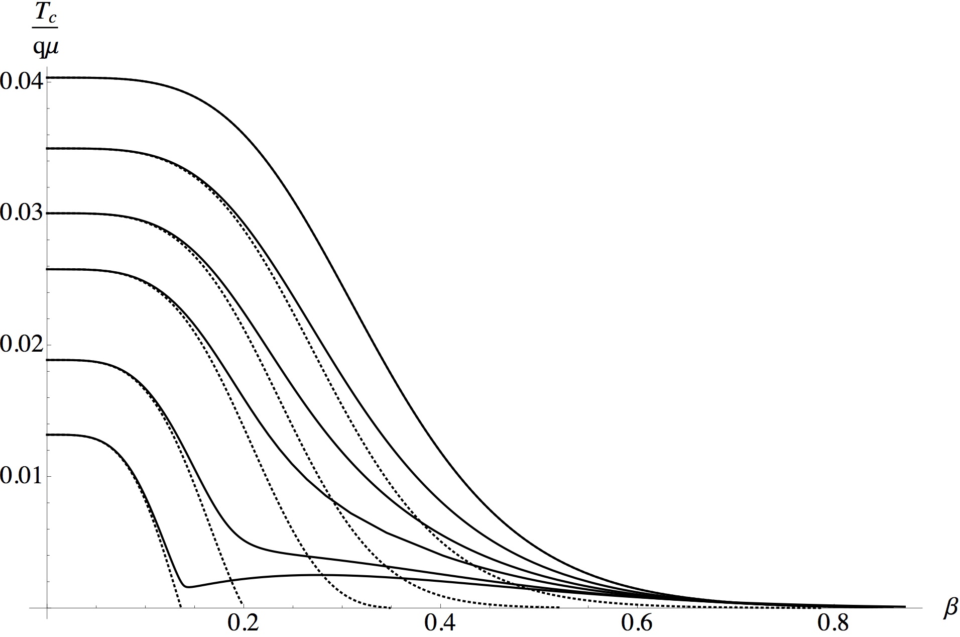
Figure 1: The critical temperature $vs.$ the magnetic field numerically calculated with $q=10$ and $\Delta=5/2$. The dotted lines are calculated with $\xi=0$ while the solid use $\xi=.10$. Starting from the top, on the vertical axis, the lines are $\frac{Q^{2}}{(q\mu)^{2}}=0,~{}.05,~{}.10,~{}.15,~{}.25,$ and $.35$.

Evidently, if we set $Q=0$, the effect of the interaction term (24) disappears, therefore the homogeneous solution is unaltered. For $Q\neq 0$, we obtain modified solutions. The behavior is shown in figure 1. The figure also displays the effect of $Q$ on $\beta_{\mathrm{max}}$ (21) for $\xi=0$.

The interaction term (24) alters the near horizon limit of the theory so that $m^{2}\to m^{2}+Q^{2}\left(1-\xi q^{4}\beta^{4}\mu_{c}^{4}\right)$. The minimum effective charge is found to be dependent on $\xi$, as is $\beta_{\mathrm{max}}$,

$$\beta_{max}^{4}=\frac{\tilde{q}^{2}}{12\tilde{q}_{min}^{2}}\left(\frac{\tilde{q}^{2}}{\tilde{q}_{min}^{2}}-\frac{1}{q^{2}}\right),$$ (26)

where $\tilde{q}^{2}=1-\frac{6\xi Q^{2}}{q^{2}}$, and $\tilde{q}_{min}^{2}=\frac{3+2\Delta(\Delta-3)+2Q^{2}\left(1-12\xi\right)}{4}$. For a range of $\xi$, an increase in $Q$ is seen to increase $\beta_{\mathrm{max}}$. The modifications are most pronounced for large $\beta$ leading to temperatures which are higher than the critical temperature of the corresponding homogeneous solution. Figure 2 displays the effect of the potential on the homogeneous solution as well as two inhomogeneous cases.

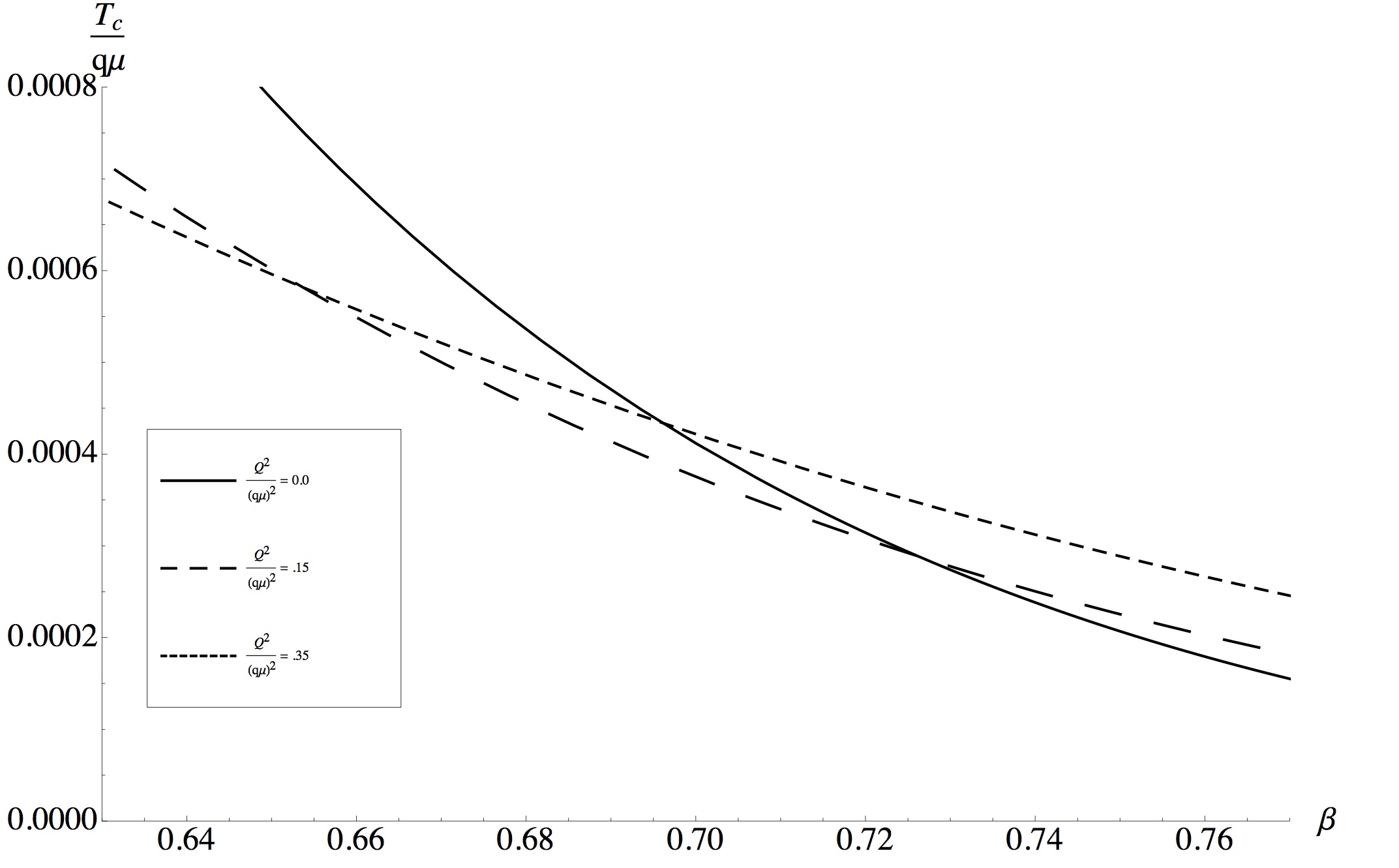
Figure 2: The top line on the left-hand side of the graph corresponds to the homogeneous solution, with lines $\frac{Q^{2}}{(q\mu)^{2}}=.15,.35$ below. The critical temperature of the homogeneous solution is found to decrease below the inhomogeneous lines for large $\beta$. We used $q=10$, $\Delta=5/2$, and $\xi=.10$.

In conclusion, we have developed a gravitational dual theory for the FFLO state of condensed matter. The gravitational theory consists of two $U(1)$ gauge fields and a scalar coupled to a charged AdS black hole. The first gauge field produces the instability for a condensate to form, while the second controls the paramagnetic effect. In the absence of an interaction of the magnetic field with the scalar field, the system possesses dominant homogeneous solutions for all allowed values of the magnetic field. In the presence of the interaction term, at low temperatures, the system is shown to possess a higher critical temperature for a scalar field with spatial modulation compared to the homogeneous solution.

Acknowledgments. This work is dedicated to the memory of our collaborator in this work, Petros Skamagoulis. We wish to thank Stefanos Papanikolaou for illuminating discussions. J. A. acknowledges support from the Office of Research at the University of Michigan-Flint. G. S. is supported by the US Department of Energy under grant DE-FG05-91ER40627.

References

- (1) S. A. Hartnoll, C. P. Herzog, and G. T. Horowitz, Phys. Rev. Lett. 101, 031601 (2008); S. A. Hartnoll, C. P. Herzog, and G. T. Horowitz, JHEP 0812, 015 (2008).
- (2) S. Bhattacharyya, V. E. Hubeny, S. Minwalla and M. Rangamani, JHEP 0802, 045 (2008).
- (3) M. Cubrovic, J. Zaanen and K. Schalm, Science 325, 439 (2009).
- (4) A. Aperis, P. Kotetes, E. Papantonopoulos, G. Siopsis, P. Skamagoulis and G. Varelogiannis, Phys. Lett. B 702, 181 (2011).
- (5) R. Flauger, E. Pajer and S. Papanikolaou, Phys. Rev. D 83, 064009 (2011).
- (6) J. A. Hutasoit, S. Ganguli, G. Siopsis and J. Therrien, JHEP 1202, 086 (2012).
- (7) S. Ganguli, J. A. Hutasoit and G. Siopsis, arXiv:1205.3107 [hep-th].
- (8) A. Donos and J. P. Gauntlett, JHEP 1108, 140 (2011).
- (9) R. Casalbuoni and G. Nardulli, Rev. Mod. Phys. 76, 263 (2004).
- (10) P. Fulde and R. A. Ferrell, Phys. Rev. 135, A550 (1964).
- (11) A. I. Larkin and Y. N. Ovchinnikov, Zh. Eksp. Teor. Fiz. 47, 1136 (1964) [Sov. Phys. JETP 20, 762 (1965)].
- (12) T. Albash and C. V. Johnson, JHEP 0809, 121 (2008).
- (13) T. Albash and C. V. Johnson, Phys. Rev. D 80, 126009 (2009); T. Albash and C. V. Johnson, arXiv:0906.0519 [hep-th].
- (14) M. Montull, A. Pomarol and P. J. Silva, Phys. Rev. Lett. 103, 091601 (2009).
- (15) K. Maeda, M. Natsuume and T. Okamura, Phys. Rev. D 81, 026002 (2010).
- (16) X. -H. Ge, B. Wang, S. -F. Wu and G. -H. Yang, JHEP 1008, 108 (2010).
- (17) F. Bigazzi, A. L. Cotrone, D. Musso, N. P. Fokeeva and D. Seminara, JHEP 1202, 078 (2012).
- (18) A. I. Buzdin, Rev. Mod. Phys. 77, 935 (2005).
- (19) P. Breitenlohner and D. Z. Freedman, Annals Phys. 144, 249 (1982).
- (20) G. T. Horowitz and M. M. Roberts, JHEP 0911, 015 (2009).
- (21) J. Alsup, G. Siopsis, and J. Therrien, Phys. Rev. D 86, 025002 (2012).
- (22) B. S. Chandrasekhar, Appl. Phys. Lett. 1, 7 (1962). A. M. Clogston, Phys. Rev. Lett. 9, 266 (1962).