Transport through single-level systems: Spin dynamics in the nonadiabatic regime

Abstract

We investigate the Fano-Anderson model coupled to a large ensemble of spins under the influence of an external magnetic field. The interaction between the two spin systems is treated within a meanfield-approach and we assume an anisotropic coupling between these two systems. By using a nonadiabatic approach, we make no further approximations in the theoretical description of our system, apart from the semiclassical treatment. Therewith, we can include the short-time dynamics as well as the broadening of the energy levels arising due to the coupling to the external electronic reservoirs. We study the spin dynamics in the regime of low and high bias. For the infinite bias case, we compare our results to those obtained from a simpler rate equation approach, where higher-order transitions are neglected. We show, that these higher-order terms are important in the range of low magnetic field. Additionally, we analyze extensively the finite bias regime with methods from nonlinear dynamics, and we discuss the possibility of switching of the large spin.

I Introduction

A quantum dot typically consists of $10^{5}$ atoms. Electrons tunneling through such devices experience hyperfine and spin-orbit interaction with the nuclear spins of the host material.Hanson2007 ; Erlingsson2005 ; Baugh2007 Combinations of huge numbers of spins can be described as a large external effective spin system which interacts with the single electron spin. In experiments with quantum dots, features such as a large Overhauser field Baugh2007 and self-sustained current oscillations have been observed.Ono2004

The effects of spin-orbit and hyperfine coupling is within the scope of recent research for various kinds of systems, such as self-assembled quantum dots, Takahashi2010 ; Hamaya2008 carbon nanotubes Hauptmann2008 or molecular magnets.Jo2006 ; Heersche2006 ; Bogani2008 ; Misiorny2009 ; Friedmann2010 ; Bode2012 The latter are promising candidates for spintronics.Thomas1996

The interaction of electron spins with a large spin reveals interesting nonlinear effects, and the system is known to exhibit chaotic behavior.Feingold1983 ; Peres1984 ; Peres1984b ; Robb1998 These effects appear for a closed system with anisotropic coupling and an external magnetic field. López-Moniz and co-workers Lopez-Monis2012 discussed the coupling to two external leads, which were assumed to be polarized. Within a rate equation approach, they found that the chaotic behavior survives for small magnetic fields.

Using a nonadiabatic approach in this paper, we extend this approach to the finite bias regime, which is not accessible within the rate equation method. Furthermore, the rate equations method is also restricted to first-order transitions, which we also extend with our nonadiabatic approach.

The nonadiabatic approach works well for systems whose quantum fluctuations are assumed to be small and that are coupled to a nonequilibrium environment. Here, we adopt this method (that we had extensively tested for nanoelectromechanical systems Metelmann2011 ) to the more complex situation of a collective spin instead of an oscillator variable. This semiclassical description is suitable for these systems as long the number of spins, which build up the ensemble, is comparatively large.Schuetz2012 ; Mosshammer2012 ; Morrison2008 ; Morrison2008a ; Ribeiro2008 For a further analysis of correlations between the spin states, for instance to study entanglement of the ensemble and the single electron spin, a quantum description is certainly required. Rudner2010 However, within a semiclassical description, it is possible to discuss the main spin dynamics. Even though the nuclear spin dynamics can be assumed to be slower than the electron spin dynamics, Hanson2007 ; Bode2012 we found that in certain parameter regimes an adiabatic approximation is not sufficient to describe the system’s dynamics.

Our paper starts with a detailed description of the model and the adaptation of the nonadiabatic approach. We directly derive the rate equation approach from our nonadiabatic method, which is presented in Sec. II.2. Afterwards, we compare the results of both methods in the infinite bias regime. In Sec. III we start the investigation of the finite bias regime with a dynamical analysis based on an adiabatic approach with Green’s functions. Therewith we interpret the nonadiabatic results for the spin dynamics. Within our conclusion in Sec. IV, we discuss the advantages and disadvantages of the methods used here.

II Model

We assume that a vertical magnetic field $B_{z}$ is applied to a Fano-Anderson model.Anderson1961 ; Fano1961 The magnetic field leads to a Zeemann splitting of the electronic level $\varepsilon_{d}$ into two levels,Zeemann1897 corresponding to $\varepsilon_{\sigma}=\varepsilon_{d}\pm\frac{1}{2}B_{z}$, with $\sigma\in\uparrow,\downarrow$. Without further interactions, this solely leads to two spin-dependent current channels. Only electrons with spin-up (-down) can tunnel through the upper (lower) energy level. These energy levels are broadened due to the coupling to the leads, and for small magnetic fields an overlap of both channels exists, but there is no communication arranged between the two energy levels, and spin-flips cannot occur. Here we enable transitions between the two energy levels with the help of a large external spin, which interacts with the electronic spin.

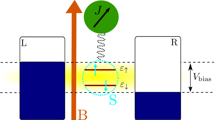
Figure 1: Sketch of a single-level system coupled to a large external spin J. Here S denotes the electronic spin and B the external magnetic field. The detuning of the leads’ chemical potentials leads to a transport window in the size of the applied bias $V_{\rm bias}$.

Fig. 1 depicts a sketch of the considered model. There, $\mathbf{\hat{S}}$ denotes the electronic spin operator for the levels, which components are defined via

$$\hat{S}_{x}= \frac{1}{2}\left(\hat{d}^{{\dagger}}_{\uparrow}\hat{d}_{\downarrow}^{\phantom{{\dagger}}}+\hat{d}^{{\dagger}}_{\downarrow}\hat{d}_{\uparrow}^{\phantom{{\dagger}}}\right),$$

$$\hat{S}_{y}= \frac{1}{2i}\left(\hat{d}^{{\dagger}}_{\uparrow}\hat{d}_{\downarrow}^{\phantom{{\dagger}}}-\hat{d}^{{\dagger}}_{\downarrow}\hat{d}_{\uparrow}^{\phantom{{\dagger}}}\right),$$

$$\hat{S}_{z}= \frac{1}{2}\left(\hat{d}^{{\dagger}}_{\uparrow}\hat{d}_{\uparrow}^{\phantom{{\dagger}}}-\hat{d}^{{\dagger}}_{\downarrow}\hat{d}_{\downarrow}^{\phantom{{\dagger}}}\right),$$ (1)

introducing the creation/annihilation operators $\hat{d}^{{\dagger}}_{\sigma}/\hat{d}_{\sigma}^{\phantom{{\dagger}}}$ of the electronic levels. The vertical magnetic field $B_{z}$ couples to the $\hat{S}_{z}$ operator, leading to the splitting of the initial single level. The Hamiltonian for the Fano-Anderson model reads

$$\mathcal{H}_{\rm{FA}}= \sum_{\sigma}\varepsilon_{d}\ \hat{d}^{{\dagger}}_{\sigma}\hat{d}_{\sigma}^{\phantom{{\dagger}}}+\sum_{k\alpha\sigma}\varepsilon_{k\alpha\sigma}\hat{c}_{k\alpha\sigma}^{{\dagger}}\hat{c}_{k\alpha\sigma}^{\phantom{{\dagger}}}$$

$$+\sum_{k\alpha\sigma}\left(V_{k\alpha\sigma}\hat{c}_{k\alpha\sigma}^{{\dagger}}\hat{d}_{\sigma}^{\phantom{{\dagger}}}+V^{\ast}_{k\alpha\sigma}\hat{d}^{{\dagger}}_{\sigma}\hat{c}_{k\alpha\sigma}^{\phantom{{\dagger}}}\right)+B_{z}\hat{S}_{z}.$$ (2)

Note, that the left ($\alpha=\rm L$) and right ($\alpha=\rm R$) lead operators $\hat{c}^{{\dagger}}_{k\alpha\sigma}/\hat{c}_{k\alpha\sigma}^{\phantom{{\dagger}}}$ are spin-dependent. This enables us to consider polarized leads, where the density of states for spin-up and spin-down electrons with energy $\varepsilon_{k\alpha\sigma}$ differs. This could be realized with ferromagnetic leads,Hamaya2008 ; Hofstetter2010 ; Sothmann2010 ; Weymann2005 leading to a spin-dependent current through the system. The third term in the Hamiltonian describes the transitions between a state in the lead and the electronic levels with tunneling amplitude $V_{k\alpha\sigma}$. For simplicity, we include the prefactor of the last term in Eq. (II), containing the electronic $g$-factor, into the definition of the magnetic field.

In addition to the electronic spin operators, the large external spin’s $z$-component $\hat{J}_{z}$ couples to the magnetic field. The free motion for it is described by

$$\mathcal{H}_{J}=B_{z}\hat{J}_{z},$$ (3)

where we assume the same g-factor and therewith the same magnetic field as for the electronic spin operators. This is a simplification in theoretical approaches, cf. Lopez-Monis2012 ; Bode2012 , but a generalization is straightforward.

Here, a large external spin means an effective spin describing a big ensemble of spins, for example, the collective spin of the nuclei in a quantum dot or a molecule. Electrons which tunnel through such devices, experience an interaction with the effective spin of the whole system. This interaction is described by Slicher1990 ; Hanson2007

$$\hat{V}=\sum_{i}\lambda_{i}\ \hat{S}_{i}\hat{J}_{i},\hskip 28.45274pti=x,y,z;$$ (4)

introducing the coupling constant $\lambda_{i}$. If these coupling constants are equal for all components $\lambda_{i}=\lambda_{j}$, one speaks of an isotropic coupling, corresponding to the Fermi contact term in the hyperfine interaction. The latter is important for spin-spin interactions in quantum dots, i.e. in GaAs dots due to their s-type conduction band.Cerletti2005 In a realistic quantum dot model the electron wave function is not uniform over the nuclei side and the coupling between the individual spins is varying, but it can be assumed to be piecewise flat in a large spin model.Rudner2010

In this paper we consider the anisotropic case in which interesting dynamical behavior was observed.Robb1998 There, at least for two components, $\lambda_{i}\neq\lambda_{j}$ is valid. An anisotropic coupling is relevant for systems with higher angular momentum bands where an enhancement of the anisotropic hyperfine interaction appears and the isotropic interaction vanishes.Coish2009 The anisotropic hyperfine interaction appears, for example, in carbon nanotubes or graphene,Fischer2009 as well as in molecular magnets.

We treat the interaction of the two spins in a semiclassical manner. Therefore, we have to assume that the quantum fluctuations in the system are small. This should be valid as long as the external spin is large and its fluctuation can be neglected. As a consequence of this assumption, we have no spin decay due to dissipation, and the large spin’s length $j$ is conserved.

Using a mean-field approximation Lopez-Monis2012 for Eq. (4) we obtain

$$\hat{V}_{\rm{MF}}=\sum_{i}\lambda_{i}\left(\hat{S}_{i}\ \langle\hat{J}_{i}\rangle+\hat{J}_{i}\ \langle\hat{S}_{i}\rangle-\langle\hat{S}_{i}\rangle\ \langle\hat{J}_{i}\rangle\right),i=x,y,z.$$ (5)

Thereby, the fluctuations $\delta\hat{A}_{i}=\hat{A}_{i}-\langle\hat{A}_{i}\rangle,\hat{A}\in\hat{S},\hat{J}$ have been neglected. Now we can build up a closed system of equations for the considered system.

For the large spin we use the commutation relations to derive the Heisenberg equations of motion

$$\frac{d}{dt}\langle\hat{J}_{x}\rangle =-\left(\lambda_{z}\langle\hat{S}_{z}\rangle+B_{z}\right)\langle\hat{J}_{y}\rangle+\lambda_{y}\langle\hat{S}_{y}\rangle\langle\hat{J}_{z}\rangle,$$

$$\frac{d}{dt}\langle\hat{J}_{y}\rangle =\hskip 11.38092pt\left(\lambda_{z}\langle\hat{S}_{z}\rangle+B_{z}\right)\langle\hat{J}_{x}\rangle-\lambda_{x}\langle\hat{S}_{x}\rangle\langle\hat{J}_{z}\rangle,$$

$$\frac{d}{dt}\langle\hat{J}_{z}\rangle =\hskip 14.22636pt\lambda_{x}\langle\hat{S}_{x}\rangle\langle\hat{J}_{y}\rangle-\lambda_{y}\langle\hat{S}_{y}\rangle\langle\hat{J}_{x}\rangle.$$ (6)

This is a strongly nonlinear system, since the values of the electronic spin components depend on the large spin.

The treatment of the electronic spin plays a decisive role in the theoretical description of this system. By using a rate equation approach, the electronic spin components are obtained from equations of motions similar to Eq. (II). Therewith, the short-time dynamics is included, but the contributions of the leads come in only as rates. Following from that, higher-order transitions are neglected and one is restricted to the infinite bias regime. One way of including higher-order transitions is by applying an adiabatic approximation, where the movement of the large spin is assumed to be slow compared to changes in the electronic subsystem. The electronic spin operators can then be derived via Keldysh Green’s functions keldysh1965 ; Kamenev2009 ; Haug2008 and are given in explicit expressions. The disadvantage of this method is that the short-time dynamics is missing.

In the next part of this paper we derive equations of motion for the electronic spin operators using a completely nonadiabatic approach. The latter enables us to include the short-time dynamics as well as higher-order transitions. Following from that, we can probe the rate equation and the adiabatic approach.

II.1 Nonadiabatic approach

In the framework of the nonadiabatic approach, we calculate all system quantities by considering their full time-dependence. In the following, we assume an anisotropic coupling $\lambda_{y}=0$ and $\lambda_{x}=\lambda_{z}=\lambda$, and together with the mean-field approach, we obtain an effective Hamiltonian for the electronic levels,

$$\mathcal{H}_{\rm{c}}(t)\equiv \sum_{\sigma}\varepsilon_{\sigma}(t)\ \hat{d}^{{\dagger}}_{\sigma}\hat{d}_{\sigma}^{\phantom{{\dagger}}}+\frac{\lambda}{2}\langle\hat{J}_{x}(t)\rangle\left(\hat{d}^{{\dagger}}_{\uparrow}\hat{d}_{\downarrow}^{\phantom{{\dagger}}}+\hat{d}^{{\dagger}}_{\downarrow}\hat{d}_{\uparrow}^{\phantom{{\dagger}}}\right)+\mathcal{H}_{\rm T},$$

$$\varepsilon_{\sigma}(t)\equiv \ \varepsilon_{d}\pm\frac{B_{z}}{2}\pm\frac{\lambda}{2}\langle\hat{J}_{z}(t)\rangle,\hskip 14.22636pt\sigma=\uparrow,\downarrow.$$ (7)

The term $\mathcal{H}_{\rm T}$ contains the coupling to the leads. Based on this effective Hamiltonian, we can describe the effects arising due to the coupling to a large external spin. The $\langle\hat{J}_{z}(t)\rangle$ - component solely leads to an additional shift of the electronic levels,Koenemann2012 but the coupling to the $\langle\hat{J}_{x}(t)\rangle$ - component enables transitions between both levels. This Hamiltonian corresponds to a two-level or a parallel double-dot system,Mourokh2002 ; Brandes2005 where the prefactor $\frac{\lambda}{2}\langle\hat{J}_{x}(t)\rangle$ would be equivalent to a time-dependent tunneling amplitude between the two (dot) levels $\varepsilon_{\uparrow}$ and $\varepsilon_{\downarrow}$.

The derivation of the equations of motion for the spin operators is performed starting from the Heisenberg equations of motion. The derivation is similar to those used before for the description of nanoelectromechanical systems, for details see Ref.Metelmann2011 . The probability for a transition between lead $\alpha$ and the electronic level $\varepsilon_{\sigma}$ for an electron with energy $\omega(\hbar\equiv 1)$ and spin $\sigma$ is described by the spin dependent tunneling rates $\Gamma_{\alpha\sigma}(\omega)$ obtained from Fermi’s Golden rule. We use a flat band approximation leading to energy-independent rates $\Gamma_{\alpha\sigma}=2\pi\sum_{k}\left|V_{k\alpha\sigma}\right|^{2}\delta(\omega-\varepsilon_{k\alpha\sigma})$. Finally, the results for the spin operator expectation values yield $(\Gamma\equiv\Gamma_{\sigma}=\sum_{\alpha}\Gamma_{\alpha\sigma}$)

$$\frac{d}{dt}\langle\hat{S}_{x}(t)\rangle= -\Gamma\langle\hat{S}_{x}(t)\rangle-\left(B_{z}+\lambda\langle\hat{J}_{z}(t)\rangle\right)\langle\hat{S}_{y}(t)\rangle$$

$$+\sum_{\alpha}\int d\omega\mbox{Re}\left[\mathcal{T}^{\alpha}_{\uparrow\downarrow}(\omega,t)+\mathcal{T}^{\alpha}_{\downarrow\uparrow}(\omega,t)\right],$$

$$\frac{d}{dt}\langle\hat{S}_{y}(t)\rangle= -\Gamma\langle\hat{S}_{y}(t)\rangle+\left(B_{z}+\lambda\langle\hat{J}_{z}(t)\rangle\right)\langle\hat{S}_{x}(t)\rangle$$

$$-\lambda\langle\hat{J}_{x}(t)\rangle\langle\hat{S}_{z}(t)\rangle$$

$$+\sum_{\alpha}\int d\omega\mbox{Im}\left[\mathcal{T}^{\alpha}_{\uparrow\downarrow}(\omega,t)-\mathcal{T}^{\alpha}_{\downarrow\uparrow}(\omega,t)\right],$$

$$\frac{d}{dt}\langle\hat{S}_{z}(t)\rangle= -\Gamma\langle\hat{S}_{z}(t)\rangle+\lambda\langle\hat{J}_{x}(t)\rangle\langle\hat{S}_{y}(t)\rangle$$

$$+\sum_{\alpha}\int d\omega\mbox{Re}\left[\mathcal{T}^{\alpha}_{\uparrow\uparrow}(\omega,t)-\mathcal{T}^{\alpha}_{\downarrow\downarrow}(\omega,t)\right],$$ (8)

with the definition

$$\mathcal{T}_{\sigma\sigma^{\prime}}^{\alpha}(\omega,t)\equiv i\sum_{k}V_{k\alpha\sigma}\delta(\omega-\varepsilon_{k\alpha\sigma})e^{i\varepsilon_{k\alpha\sigma}t}\langle\hat{c}^{{\dagger}}_{k\alpha\sigma}(0)\hat{d}_{\sigma^{\prime}}(t)\rangle,$$ (9)

for the lead-transition functions

$$\frac{d}{dt}\mathcal{T}^{\alpha}_{\sigma\sigma}(\omega,t)= -i(\varepsilon_{\sigma}(t)-\omega-\frac{i}{2}\Gamma)\mathcal{T}^{\alpha}_{\sigma\sigma}(\omega,t)$$

$$-i\frac{\lambda}{2}\langle\hat{J}_{x}(t)\rangle\mathcal{T}^{\alpha}_{\sigma\sigma^{\prime}}(\omega,t)+\frac{\Gamma_{\alpha\sigma}}{2\pi}f_{\alpha}(\omega),$$

$$\frac{d}{dt}\mathcal{T}^{\alpha}_{\sigma\sigma^{\prime}}(\omega,t)= -i(\varepsilon_{\sigma^{\prime}}(t)-\omega-\frac{i}{2}\Gamma)\mathcal{T}^{\alpha}_{\sigma\sigma^{\prime}}(\omega,t)$$

$$-i\frac{\lambda}{2}\langle\hat{J}_{x}(t)\rangle\mathcal{T}^{\alpha}_{\sigma\sigma}(\omega,t),$$ (10)

where the function for equal spins $T^{\alpha}_{\sigma\sigma}$ couples to the one for different spins $T^{\alpha}_{\sigma\sigma^{\prime}}$ and vice versa. The time-dependent $z$-component of the large spin is included into the effective levels $\varepsilon_{\sigma}(t)$, cf. Eq. (II.1). Here, the Fermi function $f_{\alpha}(\omega)$ does not depend on the spin due to the assumption, that the chemical potentials for spin-up and -down electrons in each lead are equal.

For the numerical calculations, we decompose the $\mathcal{T}^{\alpha}_{\sigma\sigma}$ into their real and imaginary part and discretize the integration over the lead energies in $N$ intervals. Therefore, we obtain $\left[6+16(N+1)\right]$ coupled equations, including the equations of motion for the large spin, cf. Eq. (II).

Using the definitions for the lead-transition functions Eq. (II.1), the electronic current is obtained from

$$\mathcal{I}_{\alpha\sigma}(t) =e\ \left\{\int d\omega\ 2\ \mbox{Re}\left[\mathcal{T}^{\alpha}_{\sigma\sigma}(\omega,t)\right]-\Gamma_{\alpha\sigma}\langle\hat{n}_{\sigma}(t)\rangle\right\},$$ (11)

where $e$ equals the electron charge and the equation of motion for the occupation yields

$$\frac{d}{dt}\langle\hat{n}_{\sigma}(t)\rangle= -\Gamma\langle\hat{n}_{\sigma}(t)\rangle\pm\lambda\langle\hat{J}_{x}(t)\rangle\langle\hat{S}_{y}(t)\rangle$$

$$+\sum_{\alpha}\int d\omega\ 2\ \mbox{Re}\left[\mathcal{T}^{\alpha}_{\sigma\sigma}(\omega,t)\right].$$ (12)

Here, the upper (lower) sign refers to $\uparrow(\downarrow)$ - electrons. Note, that the total occupation number of the dot $\langle\hat{N}(t)\rangle=\langle\hat{n}_{\uparrow}(t)\rangle+\langle\hat{n}_{\downarrow}(t)\rangle$ still couples to the spin operators via the transition functions. In the next section we derive a rate equation approach in which this dependence is omitted.

II.2 Infinite bias: rate equation approach

We recover previous results for this model Lopez-Monis2012 by applying an adiabatic approximation to our approach. In concrete terms, we assume the large spin’s movement as slow compared to the electrons which are entering the system. As a consequence, we neglect the time-dependence of the large spin in the equations for the lead-transition functions Eq. (II.1), leading to $\varepsilon_{\sigma}(t)\equiv\varepsilon_{\sigma}$ and a decoupling from the equations for the large spin, $\langle\hat{J}_{x}(t)\rangle\equiv\langle\hat{J}_{x}\rangle$. The remaining two coupled equations can be solved via a Laplace transformation. Note, that this method is not a complete adiabatic approach, because in the end we still solve equations of motions for the electronic spin components, which is not the case for a full adiabatic ansatz.

Starting from Eq. (II.1) we obtain for $t\rightarrow\infty$

$$\mathcal{T}^{\alpha}_{\sigma\sigma}(\omega) =\frac{\Gamma_{\alpha\sigma}}{2\pi}f_{\alpha}(\omega)\frac{-i(\varepsilon_{\sigma^{\prime}}-\omega-\frac{i}{2}\Gamma)}{N(\omega)},$$

$$\mathcal{T}^{\alpha}_{\sigma\sigma^{\prime}}(\omega) =\frac{\Gamma_{\alpha\sigma}}{2\pi}f_{\alpha}(\omega)\frac{i\frac{\lambda}{2}\langle\hat{J}_{x}\rangle}{N(\omega)}.$$ (13)

with $N(\omega)=(\varepsilon_{\sigma^{\prime}}-\omega-\frac{i}{2}\Gamma)(\varepsilon_{\sigma}-\omega-\frac{i}{2}\Gamma)-\frac{\lambda^{2}}{4}\langle\hat{J}_{x}\rangle^{2}$. Before inserting these results into the equations for the spin operators Eq. (II.1), we separate them into real and imaginary parts and perform the integrations over $\omega$. Hence, the spin operator equations become

$$\frac{d}{dt}\langle\hat{S}_{x}(t)\rangle= -\Gamma\langle\hat{S}_{x}(t)\rangle-\left(B_{z}+\lambda\langle\hat{J}_{z}(t)\rangle\right)\langle\hat{S}_{y}(t)\rangle,$$

$$\frac{d}{dt}\langle\hat{S}_{y}(t)\rangle= -\Gamma\langle\hat{S}_{y}(t)\rangle+\left(B_{z}+\lambda\langle\hat{J}_{z}(t)\rangle\right)\langle\hat{S}_{x}(t)\rangle$$

$$-\lambda\langle\hat{J}_{x}(t)\rangle\langle\hat{S}_{z}(t)\rangle,$$

$$\frac{d}{dt}\langle\hat{S}_{z}(t)\rangle= -\Gamma\langle\hat{S}_{z}(t)\rangle+\lambda\langle\hat{J}_{x}(t)\rangle\langle\hat{S}_{y}(t)\rangle$$

$$+\frac{1}{2}\left(\Gamma_{\rm L\uparrow}-\Gamma_{\rm L\downarrow}\right).$$ (14)

This result coincides with Lopez-Monis2012 : the whole system has now been reduced to six coupled equations, and the current simplifies to

$$\mathcal{I}_{\alpha\sigma}(t) =e\Gamma_{\alpha\sigma}\ \left\{\delta_{\alpha\rm L}-\langle\hat{n}_{\sigma}(t)\rangle\right\},$$ (15)

with the occupation

$$\frac{d}{dt}\langle\hat{n}_{\sigma}(t)\rangle= -\Gamma\langle\hat{n}_{\sigma}(t)\rangle\pm\lambda\langle\hat{J}_{x}(t)\rangle\langle\hat{S}_{y}(t)\rangle+\Gamma_{\rm L\sigma}.$$ (16)

As mentioned before, the total occupation number of the dot, $\langle\hat{N}(t)\rangle=\sum_{\sigma}\langle\hat{n}_{\sigma}(t)\rangle$, decouples from the remaining equations and becomes constant in the long-time limit,

$$\langle\hat{N}(t\rightarrow\infty)\rangle= \frac{\left(\Gamma_{\rm L\uparrow}+\Gamma_{\rm L\downarrow}\right)}{\Gamma}.$$ (17)

The equations for the spin operators Eq. (II.2) and the large external spin Eq. (II) provide further possibilities for an analytic investigation. The fixed points of the system can easily be calculated, see Lopez-Monis2012 .

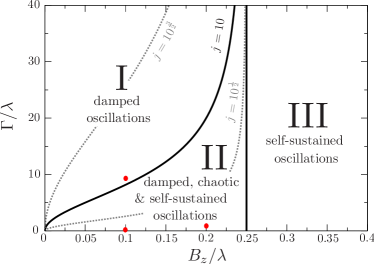
Figure 2: Regions of different dynamical behavior concerning the parameters $\Gamma$ and $B_{z}$ using the rate equation approach. As a complement, the gray lines in Fig. 2 illustrate the change of the first two regions if the length of the large spin is varied, while the ratio of the tunneling rates is fixed. For a smaller spin ($j=10^{\frac{1}{2}}$), region II decreases to the benefit of region I, which increases. Equally, the reverse situation can be seen, if the length of the spin is increased ($j=10^{\frac{3}{2}}$). Modifying the ratio of the tunneling rates shifts the vertical line separating region II from region III. The red dots denote the parameter sets for region I and II which we used in our discussion below, see Sec. II.3.

By varying the magnetic field $B_{z}$ and the tunneling rate $\Gamma$ three regions of different dynamical behavior were obtained from the rate equation approach. In Fig. 2 these regions are depicted. There, the boundary between the regions is defined via the fixed points of the system, which we introduce below. The solid black lines correspond to parameters used in. Lopez-Monis2012 There, the length of the large spin equals $j=|\hat{J}|=10$ and the tunneling rates match $2\Gamma_{\rm L\uparrow}=\Gamma_{\rm L\downarrow}=\Gamma$. This choice of tunneling rates implies $\Gamma_{\rm R\downarrow}=0$, because in this case the current flows exclusively through the upper electronic level. Following from that, spin-down electrons get trapped into the lower level and only contribute to transport after a spin-flip. Note, that $j=10$ is a relatively small value for a large spin in the semiclassical regime. A higher value of $j$ modifies the border between region I and region II, as depicted in Fig. 2, but the respective dynamical behavior in these regions stays qualitatively the same.

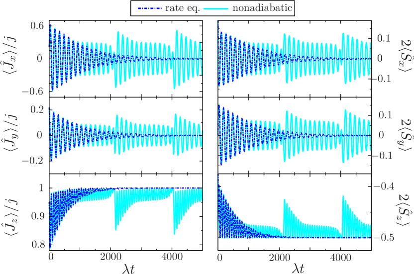
Figure 3: Comparison of the nonadiabatic approach and the rate equation approach results for regime I. The magnetic field equals $B_{z}/\lambda=0.1$ and the tunneling rate is chosen as $\Gamma/\lambda=9$. Initial conditions are $\langle\hat{J}_{x}(0)\rangle=\langle\hat{J}_{y}(0)\rangle=5(\sqrt{5}-1)/(2\sqrt{2})$ and $\langle\hat{J}_{z}(0)\rangle=5/\sqrt{2}\sqrt{5+\sqrt{5}}$ for the large spin and $\langle\hat{S}_{y}(0)\rangle=\langle\hat{S}_{z}(0)\rangle=0$ and $\langle\hat{S}_{x}(0)\rangle=0.5$ for the electronic spin.

II.3 Infinite bias (IB): results

The results for regime I are depicted in Fig. 3. The rate equation results describe damped oscillations, as expected. For large times, the $z$-component of the large spin becomes polarized parallel to the magnetic field and one spin-down electron gets trapped in the lower energy level. There the spin trajectories end up in one of the fixed points,

$$\mathcal{P}^{\pm,\rm IB}_{S0}:\langle\hat{J}_{0}\rangle=\left(0,0,\pm j\right),\hskip 5.69046pt\langle\hat{S}_{0}\rangle=\left(0,0,\frac{\Gamma_{\rm L\uparrow}-\Gamma_{\rm L\downarrow}}{2\Gamma}\right).$$ (18)

These stationary solutions exist in the whole parameter regime and are independent of the magnetic field.

In the nonadiabatic case the dynamical behavior is quite different. For small times, the spin trajectories follow the damped results from the rate equation approach. But the damping decreases strongly after the time step $t\lambda\approx 1000$. The same amount of time steps later, the amplitude drops down for one oscillation period, followed by a return to the initial oscillation. This behavior is similar for all spin components. If we consider the $z$-component for the large spin, the turning point appears when it approaches its fixed point value $\langle\hat{J}_{z,0}\rangle=j$.

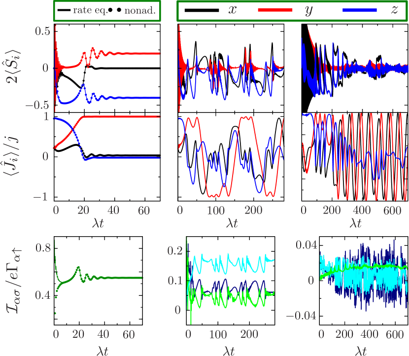
Figure 4: Behavior of the spin components in regime II. The left column depicts results for $B_{z}/\lambda=0.2$ and $\Gamma/\lambda=0.7$, where fast damping of the trajectories appears in both approaches. The middle column shows results for $B_{z}/\lambda=0.1$ and $\Gamma/\lambda=0.16$, where the rate equations predict self-sustained oscillations, but for the nonadiabatic results, already chaotic-like behavior appears. This is the same for the right column, where the tunneling rate is further reduced ($\Gamma/\lambda=0.015$). For clarity, we omitted the rate equation results for the chaotic-like regions. The lowest row depicts the corresponding current results. For the chaotic-like regions, the green line denotes $-\mathcal{I}_{\rm R\uparrow}$, the light blue line $\mathcal{I}_{\rm L\uparrow}$, and the dark blue line $\mathcal{I}_{\rm L\downarrow}$. Initial conditions are chosen as for Fig. 3.

By varying the parameters, we found no damped oscillations in region I at all. In the area close to the boundary between region I and region II, the dynamics appears as in Fig. 3. The time-interval between the turning points decreases by going away from the border and deeper into region I. By keeping the magnetic field fixed at $B_{z}/\lambda=0.1$ and increasing the tunneling rate, the trajectories perform smooth self-sustained oscillations. This transition appears near $\Gamma/\lambda\approx 11$. If we decrease the tunneling rate, the oscillations disappear around $\Gamma/\lambda\approx 8$ and we enter region II. Note that the borders between all regions defined within the rate equation approach coincide with those in the nonadiabatic approach, because the appearing fixed points are the same.

The results for regime II are depicted in Fig. 4. The rate equation approach predicts three kinds of dynamical behavior, namely strong damped, self-sustained, and chaotic oscillations.

For $B_{z}/\lambda=0.2$ and small tunneling rate $\Gamma/\lambda=0.7$ the system performs strong damped oscillations and runs into one of the fixed points $\mathcal{P}^{+,\rm IB}_{SN}(N=1,2)$,

$$\langle\hat{J}_{1,2}\rangle= \left(\frac{\Gamma}{B_{z}}\mathcal{B}_{1,2},\sqrt{j^{2}-\frac{\Gamma^{2}}{B_{z}^{2}}\mathcal{B}^{2}_{1,2}-\frac{B_{z}^{2}}{\lambda^{2}}},-\frac{B_{z}}{\lambda}\right),$$

$$\langle\hat{S}_{1,2}\rangle= \left(0,\mathcal{B}_{1,2},-\frac{B_{z}}{\lambda}\right),$$ (19)

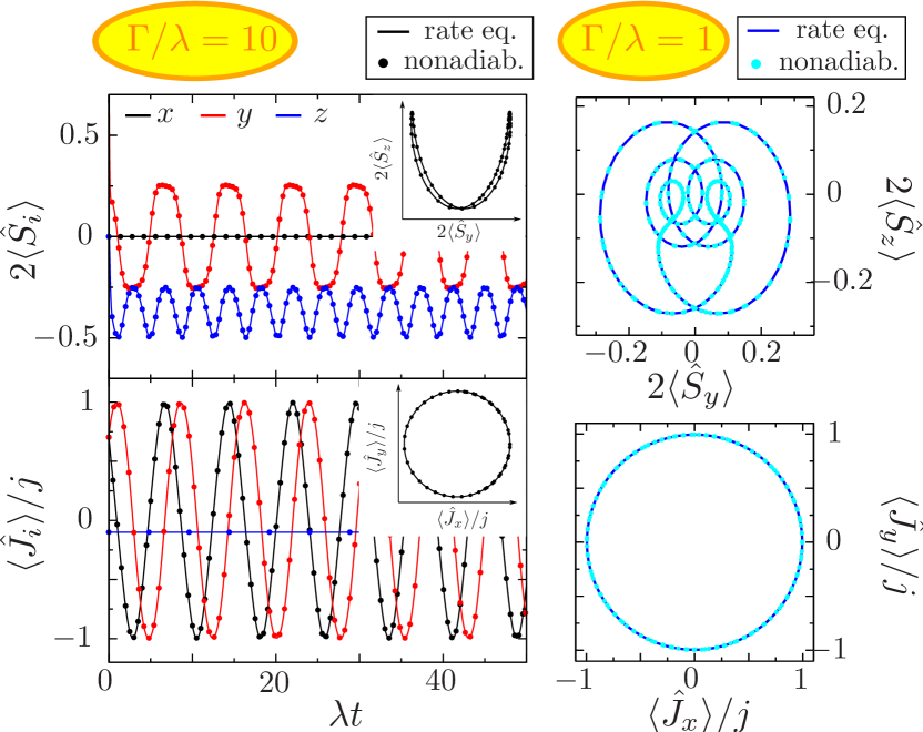
Figure 5: Results for regime III, where self-sustained oscillations appear. In the left graphs ($\Gamma/\lambda=10$) the oscillations are smoothed sinusoidal, the insets show the results in polar representation. For lower tunneling rate, the $\langle\hat{S}_{i}\rangle$ trajectories perform non-sinusoidal, but periodic oscillations, depicted in the upper graph on the right side. Parameters are $B_{z}/\lambda=1.0$, $\epsilon_{d}/\lambda=0$ and with the initial conditions $\langle\hat{J}_{x}(0)\rangle=\langle\hat{J}_{y}(0)\rangle=3\sqrt{5.5}$, $\langle\hat{J}_{z}(0)\rangle=-1$ and $\langle\hat{S}_{x}(0)\rangle=\langle\hat{S}_{z}(0)\rangle=0$, $\langle\hat{S}_{y}(0)\rangle=0.5$.

with

$$\mathcal{B}_{1,2}= \pm\sqrt{\frac{B_{z}}{\lambda}\left[\frac{\Gamma_{\rm L\downarrow}-\Gamma_{\rm L\uparrow}}{2\Gamma}-\frac{B_{z}}{\lambda}\right]}.$$ (20)

Additionally, there exist two more fixed points $\mathcal{P}^{-,\rm IB}_{SN}$ with opposite sign of the $y-$component of the large spin.

This result coincides perfectly with the nonadiabatic result, see left column in Fig. 4. The spin components run into the fixed point $\mathcal{P}^{+,\rm IB}_{S1}$, cf. Eq. (II.3). The large spin becomes almost completely polarized perpendicular to the magnetic field.

In the first instance, by further increasing the tunneling rate, the rate equations forecast self-sustained oscillations for the systems trajectories, followed by a chaotic oscillating behavior. Using the nonadiabatic approach, things change again. There, the chaotic-like behavior appears already in the parameter region, where self-sustained oscillations were predicted by the rate equation approach. Within the nonadiabatic approach, we do not recover these self-sustained oscillations in region II; we solely observe strong damping or chaotic-like behavior.

For higher values of the external magnetic field (regime III) the system performs self-sustained oscillations. The results are depicted in Fig. 5. There, the oscillation frequency of the large spin is close to the Larmor frequency $\omega_{L}=B_{z}$, which appears in our depiction at a frequency $\tilde{\omega}_{L}=B_{z}/\lambda$. In the case without coupling between the two spin systems, the large spin oscillates exactly with the frequency $\tilde{\omega}_{L}$ in the $xy-$plane. The $z$-component is fixed due to $\langle\dot{J}_{z}\rangle=0$ and possesses no coupling to the magnetic field.

The left graphs in Fig. 5, depict results for $\Gamma/\lambda=10$. Here, the frequency of the electronic spin’s $y$-component matches the frequency of the large spin’s $x$- and $y$-component $\omega_{S_{y}}=\omega_{J_{x}}=\omega_{J_{y}}\approx 0.8/\lambda$. But the $z$-component of the electronic spin is almost twice the frequency of the other components, $\omega_{S_{z}}\approx 1.6\lambda$. This behavior survives for a smaller tunneling rate, see right graphs in Fig. 5, but there the frequency is even closer to the Larmor frequency, $\omega_{J_{x},J_{y},S_{y}}\approx 0.96\lambda$ and $\omega_{S_{z}}\approx 1.91\lambda$. The appearance of the frequency doubling for $\langle\hat{S}_{z}(t)\rangle$ is explained in Sec. A.

The electronic current in regime III performs periodic oscillations. There, the results for the rate equation approach coincide with the nonadiabatic results, which are depicted in Fig. 6 for the same parameters as in Fig. 5. The frequency of the current oscillations, $\omega=2\pi/T$, matches $\omega_{S_{z}}$. Not surprising, because this spin component corresponds to the occupation difference of the dot system, $2\langle\hat{S}_{z}\rangle=\langle\hat{n}_{\uparrow}\rangle-\langle\hat{n}_{\downarrow}\rangle$. Inserting the latter into the current equation Eq. (15) and using the solution for the total occupation number in the long-time limit, cf. Eq. (17), we obtain for the current through lead $\alpha$ in the rate equation frame

$$\mathcal{I}_{\alpha}(t)= e\left[\left\{\delta_{\alpha\rm L}-\frac{\Gamma_{\rm L\uparrow}+\Gamma_{\rm L\downarrow}}{2\Gamma}\right\}(\Gamma_{\alpha\uparrow}+\Gamma_{\alpha\downarrow})\right.$$

$$\left.-\langle\hat{S}_{z}(t)\rangle(\Gamma_{\alpha\uparrow}-\Gamma_{\alpha\downarrow})\right].$$ (21)

And with $\Gamma=\Gamma_{\rm L\sigma}+\Gamma_{\rm R\sigma}$ it is obvious that $\mathcal{I}_{\rm L}(t)=-\mathcal{I}_{\rm R}(t)$ for all times $t$, and hence current conservation is ensured. The latter is also valid for the nonadiabatic approach.

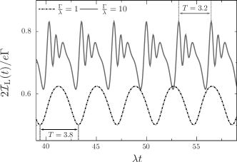
Figure 6: Nonadiabatic current results corresponding to Fig. 5. The dashed-dotted line represents the current for a small tunneling rate, where smoothed oscillations appear. For higher $\Gamma$, solid gray line, the oscillation is still periodic but not longer sinusoidal.

From the above comparison, we can already conclude, that higher-order terms in the system-lead coupling, as included in the nonadiabatic approach, do matter in the regime of low magnetic field.

III Dynamics in the finite bias regime

In the last section our investigation was focused on the infinite bias regime. There, the interaction between the large spin and the electronic system leads to interesting nonlinear effects. The rate equation approach is restricted to this regime of high external bias. With our nonadiabatic approach, we learned that differences appear if one includes higher-order transition terms. In this section, we take the next step by studying the finite bias regime.

Due to the lack of an easy access to further analytic studies for the nonadiabatic approach, we use an adiabatic approach based on Keldysh Green’s functions for the dynamical analysis; for details, see Sec. B. This enables us to clarify the effects of a finite transport window.

III.1 Dynamical analysis : adiabatic approach

Using a complete adiabatic approach for our system implies the assumption that the large spin’s movement is slower compared to the electrons jumping through the system. This is an additional assumption on top of the mean-field approach, where quantum fluctuations are neglected already. But even for the derivation of the rate equations, one needs an adiabatic approximation for the electrons tunneling into the system. We performed the latter in the preceding section to decouple the lead-transition functions, cf. Eq. (II.2). A full adiabatic approach also assumes that the electronic spin changes on a time-scale which is much smaller than that of the large spin. This approximation for the interaction between the electronic spin and the large spin reduces the number of dynamical equations to three, because only the ones for the large spin remain. The equations of motion for the electronic spin operators are solved with the help of Green’s functions.

We can use the adiabatic approach to search for fixed points and also perform a rough characterization of them. The predictions for the classification of the fixed points coincide quite well with the actually obtained nonadiabatic results. However, a complete adiabatic treatment of the system cannot capture the whole dynamics of the system. Even in the infinite bias regime, the adiabatic results do not coincide with those obtained from the rate equation or the nonadiabatic approach.

An improvement of this approach can be done by expanding the time-dependent Green’s functions to first order, as done in Ref.Bode2012 for a related system. This expansion leads to additional friction terms in the equations of motions of the large spin. Then the dynamics are described by a Landau-Lifshitz-Gilbert equation.Ralph2008

III.1.1 Fixed point analysis of $\mathcal{P}^{\pm}_{S0}$: center or saddle point

The fixed points $\mathcal{P}^{\pm}_{S0}$, where the large spin is completely polarized parallel to the magnetic field, cf. Eq. (18), appear also for the adiabatic system. But the corresponding value of the $z$-component for the electronic spin now depends on several system parameters; for zero temperature it yields

$$\langle\hat{S}_{z,0}(\pm j)\rangle =\sum_{\alpha}\left\{\frac{\Gamma_{\alpha\uparrow}}{2\pi\Gamma}\arctan\left[\frac{\mu_{\alpha}-\varepsilon_{\uparrow}(\pm j)}{\Gamma/2}\right]\right.$$

$$\left.\hskip 25.6073pt-\frac{\Gamma_{\alpha\downarrow}}{2\pi\Gamma}\arctan\left[\frac{\mu_{\alpha}-\varepsilon_{\downarrow}(\pm j)}{\Gamma/2}\right]\right\},$$ (22)

with $\varepsilon_{\uparrow,\downarrow}(j)=\varepsilon_{d}\pm 0.5(B_{z}+\lambda j)$. The $x$- and $y$-component are zero as for the rate equation approach. For infinite bias the $z$-component solely depends on the tunneling rates $\langle\hat{S}_{z,0}^{\rm{IB}}\rangle=(\Gamma_{\rm L\uparrow}-\Gamma_{\rm L\downarrow})/2\Gamma$, which coincides with Eq. (18).

For a further investigation of the fixed points, we use a linear stability analysis,Strogatz2000 where we study the Jacobian of the dynamical system around the fixed point. Some basic details of this analysis are denoted in Appendix C, including the derivation of Eq. (III.1.1).

For the fixed points $\mathcal{P}^{\pm}_{S0}$, one eigenvalue of the Jacobian (38) is zero and the two others read

$$\mathcal{E}_{2,3}^{0,\pm}= \pm i\sqrt{\mathcal{T}_{0}\left(\mathcal{T}_{0}\mp\lambda j\left.\frac{\partial\langle\hat{S}_{x}\rangle}{\partial\langle\hat{J}_{x}\rangle}\right|_{\begin{subarray}{c}\langle\hat{J}_{x,0}\rangle=0,\\ \langle\hat{J}_{z,0}\rangle=\pm j\end{subarray}}\right)},$$

with $$\ \ \mathcal{T}_{0}=\left[\lambda\langle\hat{S}_{z,0}(\pm j)\rangle+B_{z}\right].$$ (23)

Therewith, two possible realizations can appear: either the eigenvalues are purely imaginary, classifying the fixed point as a stable center, or purely real, corresponding to a saddle point. In the stable center case, the spin trajectories perform periodic oscillations around the fixed point and their amplitudes are determined by the initial conditions. In contrast, no oscillations appear if the fixed point can be classified as a saddle point, where the trajectories get repelled and approach other stable solutions of the dynamical system.

From Eq. (III.1.1) we see, that no damped oscillations around the fixed points $\mathcal{P}^{\pm}_{S0}$ are expected in the adiabatic regime, because this so-called stable spiral case would require complex eigenvalues with a finite negative real part. This missing damping is characteristic for the adiabatic results, hence this approach cannot describe the complete dynamics of the system. The latter is valid even in the infinite bias regime, since the appearing dynamical features such as self-sustained oscillations require both, positive and negative damping, Hussein2010 whereby positive damping is indicated by a positive real part of the eigenvalue.

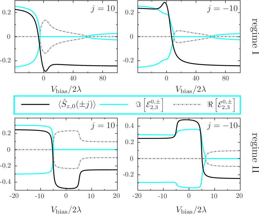
Figure 7: Results of the dynamical analysis for region I and II. Here, parameters are chosen as in Sec. II.2. The solid black line denotes the $z$-component of the electronic spin $\langle\hat{S}_{z}\rangle$ and the external bias is chosen in a symmetric manner $\mu_{\rm L}=-\mu_{\rm R}=V_{\rm bias}/2$. Zero imaginary part appears in region I for alignment of $\langle\mathbf{\hat{J}}\rangle$ in the direction of $B_{z}$ in the range of $V_{\rm bias}/2\lambda\in[-5;60]$ and for alignment in the opposite direction the range yield $V_{\rm bias}/2\lambda\in[10;60]$. For region II the imaginary part disappears in the range of $V_{\rm bias}/2\lambda\in[-5;\infty]$ for $\langle\hat{J}_{z,0}\rangle=j$ and $V_{\rm bias}/2\lambda\in[6.4;\infty]$ for $\langle\hat{J}_{z,0}\rangle=-j$.

In Fig. 7, $\langle\hat{S}_{z,0}\rangle$ as a function of the applied bias is depicted, together with the real and the imaginary part of the corresponding eigenvalue. The two upper graphs show the behavior in regime I for $\langle\mathbf{\hat{J}}\rangle$ pointing in the direction of the magnetic field (left, $j=10$) as well as against it (right, $j=-10$). We observe regions where the imaginary part of the eigenvalues is equal to zero and therewith the oscillations disappear.

The ranges of the finite real part are slightly different for $\mathcal{P}^{+}_{0}$ and $\mathcal{P}^{-}_{0}$. These differences appear for small bias; the intervals of the finite real part are denoted in the caption of Fig. 7. For $\mathcal{P}^{-}_{S0}$, the intervals with a finite real part are smaller than those for $\mathcal{P}^{+}_{S0}$. Depending on the existence of other fixed points, the regions where only one fixed point has eigenvalues with finite imaginary parts, are promising for the occurrence of spin-flips.

Based on the chosen polarization of the leads and therewith the different tunneling rates for the spin-down electrons, we obtain a system which is not symmetric. Hence, the dynamical behavior for negative detuning is different from that for positive detuning, $V_{\rm bias}>0$. This is clearly visible in Fig. 7, where for large negative bias the imaginary part in region I is always unequal to zero. The infinite bias result for region I equals $\langle\hat{S}_{z,0}\rangle^{IB}=\pm 0.25$ as expected, whereby the sign depends on the detuning. For region I, the system performs periodic oscillations for a bias $V_{\rm bias}/2\lambda>60$.

In contrast, in region II (2nd row in Fig. 7), no finite imaginary part for the high bias regime exists. This coincides with the infinite bias result for the nonadiabatic approach, where the concerned fixed points do not appear as stable centers or spirals. But here, for a small bias range and also for negative detuning, we find, that the eigenvalues can become complex and therewith the fixed points $\mathcal{P}^{\pm}_{S0}$ can exist as centers. For positive detuning, the fixed point $\mathcal{P}^{+}_{S0}$has already turned into a saddle point, but the $\langle\hat{J}_{z,0}\rangle=-10$ state is alive until $V_{\rm bias}/2\lambda=6.4$.

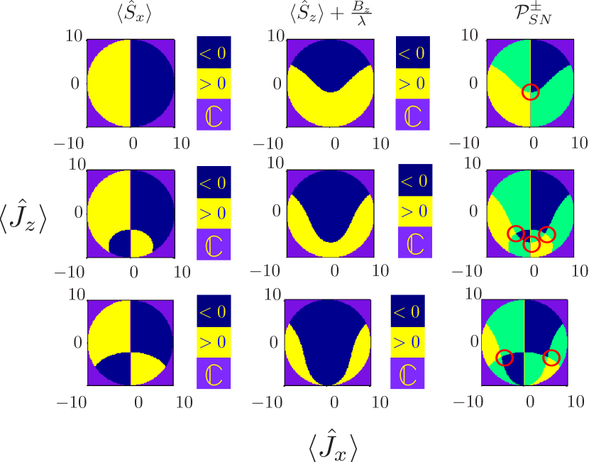
Figure 8: Results for the fixed points $\mathcal{P}^{\pm}_{SN}$ in region I: numerically calculated density plots for $\langle\hat{S}_{z}\rangle+B_{z}/\lambda$ and $\langle\hat{S}_{x}\rangle$ as a function of the large spin components. These functions must be both equal to zero for the appearance of $\mathcal{P}_{\pm}^{SN}$. The yellow (blue) area in the first two columns corresponds to positive (negative) values. Along the borders of these areas the functions are equal to zero. The right column depicts the superposition of the first two columns, there a contact of the blue and yellow area denotes a solution for $\mathcal{P}^{\pm}_{SN}$ (red circles). The bias increases from the upper to the lower row, explicit values are $V_{\rm bias}/2\lambda=5;8;10$. The numerical results were sorted by their sign, with the purpose of highlighting the positive and the negative areas. The bifurcation appears approximately at $V_{\rm bias}/2\lambda\approx 7$.

For region III, which means for $B_{z}/\lambda>0.25$, the behavior of the fixed points is similar to region I, if the magnetic field and the tunneling rate are small. But for higher values of these parameters, the real part of the eigenvalues is always zero and therewith the fixed points can be classified as stable centers with purely imaginary eigenvalues. The transition from purely real to purely imaginary eigenvalues is only numerical accessible. In Fig. 15 we depict the appearance of stable solutions as a function of the magnetic field and the tunneling rate for different bias values. In these graphs, the discussed transition is visible.

III.1.2 Two conditions for the fixed points $\mathcal{P}^{\pm}_{SN}$

The next fixed points obtained from Eq. (II) include the requirement that $\langle\hat{S}_{x}\rangle=0$ and the condition $\langle\hat{S}_{z}\rangle+B_{z}/\lambda=0$ has to be complied with as well. We define

$$\mathcal{P}^{\pm}_{SN}:\left(\langle\hat{J}_{x,N}\rangle,\pm\sqrt{j^{2}-\langle\hat{J}_{x,N}\rangle^{2}-\langle\hat{J}_{z,N}\rangle^{2}},\langle\hat{J}_{z,N}\rangle\right).$$ (24)

In the infinite bias regime $\mathcal{P}_{SN}^{\pm}$ coincide with the four fixed points $\mathcal{P}_{S1,S2}^{\pm}$ in region II, see Eq. (II.3) and below, obtained from the rate equations.

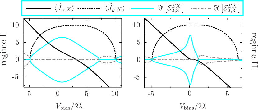
Figure 9: Results of the dynamical analysis of $\mathcal{P}^{+}_{SX}$ for region I and II. Outside of the depicted range, the fixed point is complex. The real range is limited by $\langle\hat{J}_{y,X}\rangle$, which is only real inside of the dashed line. Parameter as in Sec. II.2.

The investigation of $\mathcal{P}^{\pm}_{SN}$ in the finite bias regime is possible only numerically. In Fig. 8, we present results obtained for region I. The cycle shapes originate from the conservation of the large spin, hence the radius equals $j$. Outside of these cycles, $\langle\hat{J}_{y}\rangle$ becomes complex and no real solution for $\mathcal{P}^{\pm}_{SN}$ exists.

The stability is defined by the eigenvalues of the Jacobian (36) evaluated at $\mathcal{P}^{\pm}_{SN}$. One eigenvalue of $\mathcal{P}_{SN}^{\pm}$ is again zero, due to the fact, that we actually deal with a two-dimensional system. The remaining eigenvalues yield

$$\mathcal{E}_{2,3}^{SN}= \frac{\lambda}{2}\langle\hat{J}_{y}\rangle\left\{\left(\frac{\partial\langle\hat{S}_{x}\rangle}{\partial\langle\hat{J}_{z}\rangle}-\frac{\partial\langle\hat{S}_{z}\rangle}{\partial\langle\hat{J}_{x}\rangle}\right)\right.$$

$$\pm\left.\sqrt{\left(\frac{\partial\langle\hat{S}_{x}\rangle}{\partial\langle\hat{J}_{z}\rangle}+\frac{\partial\langle\hat{S}_{z}\rangle}{\partial\langle\hat{J}_{x}\rangle}\right)^{2}-4\frac{\partial\langle\hat{S}_{x}\rangle}{\partial\langle\hat{J}_{x}\rangle}\frac{\partial\langle\hat{S}_{z}\rangle}{\partial\langle\hat{J}_{z}\rangle}}\right\}\Bigg{|}_{\mathcal{P}^{\pm}_{SN}}.$$ (25)

For a small bias, $V_{\rm bias}/2\lambda<5$, only one solution for $\mathcal{P}^{\pm}_{SN}$ exists, corresponding to the case $\langle\hat{J}_{x,N}\rangle=0$, which we name $\mathcal{P}^{\pm}_{SX}$. The latter is stable until $V_{\rm bias}/2\lambda<7$ cf. Fig. 9. By further increasing the bias another bifurcation appears, where $\mathcal{P}^{\pm}_{SX}$ becomes unstable and two other fixed points are created. These points are symmetric to the $\langle\hat{J}_{x}\rangle$ - axis and move with higher bias values further to $\langle\hat{J}_{z}\rangle=\pm j$. When they reach the border of the cycle, they disappear and $\langle\hat{S}_{z}\rangle+Bz/\lambda=0$ no longer has a real solution. The emerging fixed points have negative/positive real eigenvalues and can be characterized as stable/unstable nodes. For region II, these points do not disappear for high bias and the nodes are the only remaining stable solutions of the system. These nodes correspond to fast damping behavior for the spin components.

For $\mathcal{P}^{\pm}_{SX}$, where $\langle\hat{J}_{x,N}\rangle\equiv\langle\hat{J}_{x,X}\rangle=0$, the last term in Eq. (III.1.2) is unequal to zero and the component $\langle\hat{J}_{z,X}\rangle$ is obtained from the transcendental equation

$$-\frac{B_{z}}{\lambda}= \sum_{\alpha}\left\{\frac{\Gamma_{\alpha\uparrow}}{2\pi\Gamma}\arctan\left[\frac{\mu_{\alpha}-\varepsilon_{d}-\frac{1}{2}(B_{z}+\lambda\langle\hat{J}_{z,X}\rangle)}{\Gamma/2}\right]\right.$$

$$\left.-\frac{\Gamma_{\alpha\downarrow}}{2\pi\Gamma}\arctan\left[\frac{\mu_{\alpha}-\varepsilon_{d}+\frac{1}{2}(B_{z}+\lambda\langle\hat{J}_{z,X}\rangle)}{\Gamma/2}\right]\right\},$$ (26)

This equation has no solution for $\langle\hat{J}_{z,N}\rangle$ in the infinite bias case and therefore the fixed points $\mathcal{P}^{\pm}_{SX}$ do not exist there. In the regime of a low magnetic field, the right side of Eq. (III.1.2) has to be small. Following from that, the argument of the $\arctan$ function has to be small as well, leading to the estimate for the evolution of the $z$-component as linear to the applied bias, $\langle\hat{J}_{z,X}\rangle\sim V_{\rm bias}$.

This linear behavior is clearly visible in Fig. 9, where we plotted $\mathcal{P}^{+}_{SX}$ and its eigenvalues as a function of the applied bias. The arcs correspond to the $\langle\hat{J}_{y,X}\rangle$ components, which determines whether the fixed point exists or not. Within these arcs, the point is real and therewith physically reasonable. The radius of the arcs are limited by the length of the large spin.

For both regions we observe small ranges with a finite imaginary part, where the fixed point can be classified as a stable center. We also observe ranges where a saddle point occurs. In regime I, the point $\mathcal{P}^{+}_{SX}$ starts its existence for $V_{\rm bias}/2\lambda\approx-5$. At this bias value, $\mathcal{P}^{+}_{S0}$ turns into a saddle point, cf. Fig. 7.

This behavior agrees quite well with that of $\mathcal{P}^{\pm}_{S0}$. We can interpret $\mathcal{P}^{\pm}_{SN}$ as the complementary points in the region, where $\mathcal{P}^{\pm}_{S0}$ disappear. As we discussed before, for a certain bias region the stable solutions $\mathcal{P}^{\pm}_{S0}$ turn into saddle points, and we can estimate, that then the fixed points appearing in Fig. 8, correspond to stable solutions of the dynamical system.

III.1.3 Fixed points for unpolarized leads

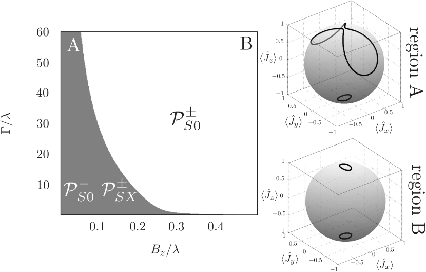
Figure 10: Fixed points for unpolarized leads as a function of tunneling rate $\Gamma$ and magnetic field $B_{z}$. The symmetric bias is chosen as $V_{\rm bias}/2\lambda=5$. The right graphs depict the adiabatic results for the large spin, in region B the small cycles on the top/bottom correspond to $\mathcal{P}^{\pm}_{S0}$. In region A, instead of $\mathcal{P}^{+}_{S0}$ the fixed point $\mathcal{P}^{+}_{SX}$ appears (larger cycle). Magnetic field for region A/B is $B_{z}/\lambda=0.1/0.3$.

For unpolarized leads, the tunneling rates become spin-independent, $\Gamma=\Gamma_{\rm L}+\Gamma_{\rm R}$. There only the fixed points $\mathcal{P}^{\pm}_{S0}$ and $P^{\pm}_{SX}$ exist, as depicted in Fig. 10. In dependence on the tunneling rate and the magnetic field, two main regions appear. The first one, region A, has the stable fixed points $\mathcal{P}^{-}_{S0}$ and $P^{\pm}_{SX}$, which can be characterized as centers. In this region, spin-flips of the large spin can be possible, because $\mathcal{P}^{+}_{S0}$ is no stable solution. But the system is still multistable, and therewith the trajectories can also end up in the fixed points $P^{\pm}_{SX}$. Note, that for a total adiabatic ansatz, a complete spin-flip is not observable, because the trajectories starting parallel to the magnetic field end up in $P^{\pm}_{SX}$, as shown in the right graphs of Fig. 10. If one reverses the direction of the magnetic field, region A contains $\mathcal{P}^{+}_{S0}$ instead of $\mathcal{P}^{-}_{S0}$.

In region B, only $\mathcal{P}^{\pm}_{S0}$ are stable fixed points. By further increasing the bias, the region where $P^{\pm}_{SX}$ exist gets smaller, and in the infinite bias case only the second region persists and all electronic spin components $\langle\hat{S}_{i}\rangle$ become zero. Then the two systems decouple and the large spin oscillates with the Larmor frequency.

III.2 Results for the nonadiabatic approach in the finite bias regime

We expect to obtain the same fixed points for the nonadiabatic approach as for the adiabatic approach. For the case $\mathcal{P}^{\pm}_{S0}$, we want to show, that these fixed points also appear in the nonadiabatic regime. There, all lead-transition functions for different spin $\mathcal{T}_{\sigma\sigma^{\prime}}^{\alpha}$ vanish in the stationary case and we obtain for the ones with equal spins the simple result

$$\mathcal{T}_{\sigma\sigma}^{\alpha}(\omega)=i\frac{\Gamma_{\alpha\sigma}}{2\pi}\frac{f_{\alpha}(\omega)}{(\omega-\varepsilon_{\sigma}(\pm j)+i\frac{\Gamma}{2})}=i\frac{\Gamma_{\alpha\sigma}}{2\pi}G^{R}_{\sigma}(\omega),$$ (27)

containing the spin-dependent single-level Green’s function $G^{R}_{\sigma}(\omega)$ without coupling of the two electronic levels, due to $\langle\hat{J}_{x,0}\rangle=0$. Also, the equation for the $z$-component of the electronic spin is straightforwardly obtained from

$$\langle\hat{S}_{z,0}\rangle= \frac{1}{\Gamma}\sum_{\alpha}\int d\omega\operatorname{Re}\left[\mathcal{T}^{\alpha}_{\uparrow\uparrow}(\omega)-\mathcal{T}^{\alpha}_{\downarrow\downarrow}(\omega)\right]$$

$$= \frac{1}{2\pi}\sum_{\sigma\alpha}\frac{\Gamma_{\alpha\sigma}}{\Gamma}\left[2\delta_{\sigma\uparrow}-1\right]\arctan\left[\frac{\mu_{\alpha}-\varepsilon_{\sigma}(\pm j)}{\Gamma/2}\right].$$ (28)

This result coincides with Eq. (III.1.1), and the fixed points are identical to the ones obtained with the adiabatic approach. In the same manner, we can construct also the other fixed points. In the general stationary case, all lead-transition functions decouple from the equation system and can be expressed by the retarded Green’s function. The adiabatic expressions for electronic spin components can also be reconstructed.

This equivalence is not valid considering the adiabatic eigenvalues; they are not directly transferable to our nonadiabatic approach. The fixed points are long-time quantities and stationary solutions of the dynamical system, in contrast the eigenvalues include higher-order terms, and their calculation requires the first derivations of the system’s variables.

But some predictions derived from the adiabatic eigenvalues also appear in the nonadiabatic approach. Therefore, we can estimate that the behavior for the full time-dependent solution is strongly influenced by the adiabatic eigenvalues.

III.2.1 Region I: Disappearance of the oscillations

We start our presentation and discussion of the nonadiabatic results with the ones obtained in region I, corresponding to a low value of the external magnetic field and a large tunneling rate. In the case of infinite bias, we obtained an oscillating behavior between two cycles. This is different from the rate equation results, where damped oscillations appear.

From the adiabatic analysis of the preceding section, we obtained the prediction, that the fixed point $\mathcal{P}^{+}_{S0}$ of the system turns from a center into a saddle point for the bias range $V_{\rm bias}/2\lambda\in[-5;60]$. When $\mathcal{P}^{+}_{S0}$ loses its stability at $V_{\rm bias}/2\lambda\approx-5$, a supercritical pitchfork bifurcation Kuznetsov ; Beuter2003 ; Strogatz2000 appears and $\mathcal{P}^{\pm}_{SX}$ are created; they exist until $V_{\rm bias}/2\lambda\approx 7$ as centers. If the latter fixed points become unstable, two stable nodes are born and we expect the oscillations to disappear. Note, that these predictions originate from the adiabatic eigenvalues.

As depicted in Fig. 11, we obtain these features also in our nonadiabatic results. There, the spin components and the current are depicted for three different bias values. For $V_{\rm bias}/2\lambda=2$, we observe non-sinusoidal self-sustained oscillations. $\langle\hat{S}_{z}\rangle$ oscillates around $-B_{z}/\lambda$, which corresponds to a stable point of kind $\mathcal{P}^{\pm}_{SX}$.

If we increase the applied bias for the initial conditions corresponding to the results depicted in Fig. 11, the oscillations disappear in the range of $V_{\rm bias}/2\lambda\approx 8$. They run into the fixed point of the kind $\mathcal{P}^{+}_{SN}$, which is clearly visible in Fig. 11, where $\langle\hat{S}_{x}\rangle=0$ and $\langle\hat{S}_{z}\rangle=-B_{z}/\lambda$.

By varying the initial conditions, we observe that not all oscillations have disappeared for a bias in the range of $V_{\rm bias}/2\lambda\approx 8$. Choosing the initial conditions near the fixed point $\mathcal{P}^{-}_{S0}$, we observe oscillations, which are smoothly sinusoidal and run around $\mathcal{P}^{-}_{S0}$. For $V_{\rm bias}/2\lambda\approx 10$, the oscillations disappear and the trajectories run in the same fixed point as depicted in the middle graph of Fig. 11. This result coincides perfectly with the border predicted in the adiabatic analysis.

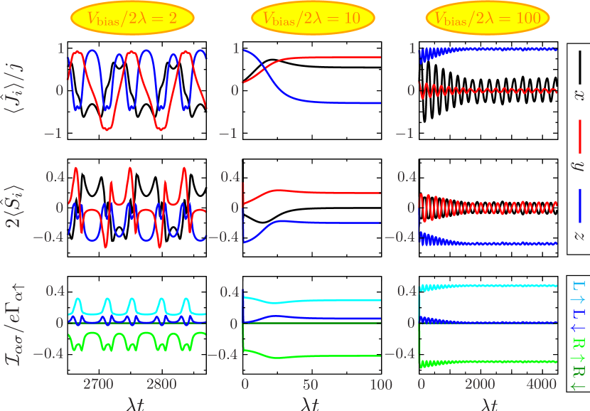
Figure 11: Nonadiabatic results obtained in region I for three different bias values, which are chosen in a symmetric manner $V_{\rm bias}=\mu_{\rm L}/2=-\mu_{\rm R}/2$. The electronic current, depicted in the lowest row, is separated into left/right and spin-up/-down contributions. The magnetic field yields $B_{z}/\lambda=0.1$ and $\Gamma/\lambda=9$. Initial conditions as in Sec. II.2 for regime I.

The bifurcation point, where a revival of the oscillations appears, is also correctly predicted by the adiabatic analysis. For $V_{\rm bias}/2\lambda\approx 60$, we observe again oscillations around $\mathcal{P}^{\pm}_{S0}$. In these oscillations, there is a slight indication of the two cycle behavior, as in the infinite bias case, but the difference between the radii of the cycles is not large. The latter is visible in the third column of Fig. 11, where the results for $V_{\rm bias}/2\lambda=100$ are depicted.

The lower row in Fig. 11 depicts the electronic current $\mathcal{I}_{\alpha\sigma}(t)$, separated into its constituent parts. The right tunneling amplitude is equal to zero, and following from that is the corresponding current channel. Therefore, the current $\mathcal{I}_{\rm R\uparrow}$ should be equal to the total current through the system, hence current conservation remains valid. For the nonadiabatic current, this is ensured for the time-averaged current values, but it can be different in the time-dependent case. There, we observed some accumulation of current in the central region.

When we consider the current channels for $V_{\rm bias}/2\lambda=2$ in Fig. 11, we notice that all channels reach their minima if the $\langle\hat{J}_{z}\rangle$-component is maximal and therewith here close to $j$. For this low bias regime, the shift of the energy level, due to the coupling to the large spin $\pm 1/2(B_{z}\lambda+\langle\hat{J}_{z}\rangle)$, leads to a positioning of the levels slightly outside of the transport window. Hence the current is minimal.

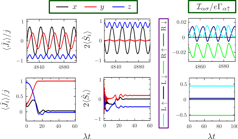
Figure 12: Nonadiabatic results for region II. The upper row corresponds to a small bias $V_{\rm bias}/2\lambda=2$, where the spin components oscillate around the coordinates of $\mathcal{P}^{-}_{S0}$. Increasing the bias, leads to a disappearing of the oscillations and one fixed point $\mathcal{P}^{+}_{SN}$ is present, see lower row for $V_{\rm bias}/2\lambda=5$. The magnetic field yields $B_{z}/\lambda=0.2$ and $\Gamma/\lambda=0.7$. Note, that the time-intervals of the current and the spin operators differ slightly. Initial conditions as in Sec. II.2 for regime I.

The current corresponding to the spin-up electrons flows in the direction of the bias. For the spin-down electrons, the situation is more complicated, because they are not allowed to leave the system through the right lead due to $\Gamma_{\rm{R}\downarrow}=0$. The electrons can either flip their spin, stay in the lower level, or flow back into the left lead. If the last process appears the electron moves against the bias and the current becomes negative. This feature is slightly visible in the lowest graph of the first column in Fig. 11, where the current $\mathcal{I}_{\rm L\downarrow}$ drops below zero for a quite small region.

Again, we can address this effect on the position of the large spin’s $z$-component. In the case $\mathcal{I}_{\rm L\downarrow}<0$, the shifting of the energy level is the other way around, because $\langle\hat{J}_{z}\rangle$ is negative. Following from that, the spin-down level lies above the spin-up level and additionally in the neighborhood of the left Fermi edge ($\mu_{\rm L}=2/\lambda$), and electrons can occupy empty states in the left lead. After $\langle\hat{J}_{z}\rangle$ passes its minima, the spin-down level moves down and therewith its current channel drops as well.

III.2.2 Region II: Negative Detuning and spin-flip of the large spin

The feature of negative current is more visible in region II, as we see in the current results for $V_{\rm bias}/2\lambda=2$, which are depicted in the upper row of Fig. 12. There, the large spin’s $z$-component oscillates close to $-j$ and therewith, both effective levels are clearly situated outside the transport window and the spin-down level lies again above the spin-up level. The oscillations of $\langle\hat{J}_{z}\rangle$ are comparatively small and do not influence the behavior of the effective levels as much as for region I. They stay outside of the transport window for all times.

We try to interpret the evolution in time for the current channels focusing on the transition between the levels. If $\mathcal{I}_{\rm L\downarrow}$ is negative, the right current reaches its minimum and the left current for spin-up electrons is maximal. Due to $\mathcal{I}_{\rm R\uparrow}<\mathcal{I}_{\rm L\uparrow}$, we can assume that spin-flips from the lower (spin-down) to the upper level (spin-up) happen, and a depletion of the upper level into the left lead appears, due to the negativity of $\mathcal{I}_{\rm L\downarrow}$. This is in accordance with the evolution for $\langle\hat{S}_{z}\rangle$, which decreases in this range.

In contrast, when $\langle\hat{S}_{z}\rangle$ increases, the left current for spin-down electrons is maximal, as well as $\mathcal{I}_{\rm R\uparrow}$. But $\mathcal{I}_{\rm L\uparrow}$ is close to zero in this regime. Therefore, we interpret this kind of current cycle in the following way. A spin-down electron enters the upper level, flips into the lower level, due to the interaction with the large spin, and finally leaves the central system to the right lead. This would explain why the current for spin-up electrons is maximal at the right lead and minimal at the left lead.

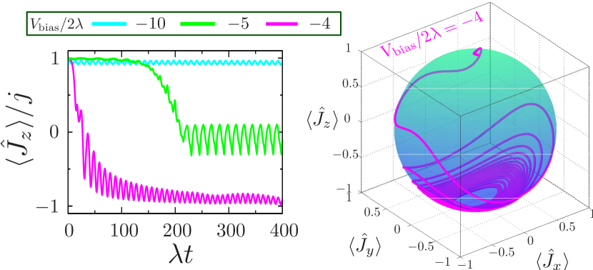
Figure 13: The large spin’s $z$-component for several bias values in regime II. Parameters as for Fig. 12, and initial conditions are $\langle\hat{J}_{x}\rangle=\langle\hat{J}_{y}\rangle=\sqrt{50-9.9^{2}/2},\langle\hat{J}_{z}\rangle=9.9$ and $\langle\hat{S}_{y}\rangle=\langle\hat{S}_{z}\rangle=0,\langle\hat{S}_{x}\rangle=0.5$.

If the bias is increased, the regions of negative spin-down current vanish, as do the oscillations of the spin components, as depicted in the lower row of Fig. 12. Remember, for the infinite bias regime, we found no periodic oscillations at all in this region. In accordance with the foregoing adiabatic analysis, the trajectories enter one fixed point of the kind $\mathcal{P}^{\pm}_{SN}$.

The adiabatic analysis, also predicts an earlier disappearance of the fixed point $\mathcal{P}^{+}_{S0}$ than the fixed point $\mathcal{P}^{-}_{S0}$. As a result, we propose the possibility of spin-flips for the large spin in the region, where only the eigenvalues of $\mathcal{P}^{-}_{S0}$ have a finite imaginary part: $V_{\rm bias}/2\lambda\in[-5;6.4]$.

To monitor how the first fixed point disappears, we choose our initial conditions close to $\mathcal{P}^{+}_{S0}$ and assume negative detuning. The results are depicted in Fig. 13. For $V_{\rm bias}/2\lambda=-10$, the trajectories perform smooth oscillations around $\mathcal{P}^{+}_{S0}$. As expected from Fig. 7, the $z$-component of the electronic spin $\langle\hat{S}_{z}\rangle\approx 0.2$ and is therewith positive. As discussed in the last section, the observed system is not symmetric and hence the fixed point $\mathcal{P}^{+}_{S0}$ stays alive by further decreasing the bias.

Increasing the bias, we see a different behavior, i.e., $\langle\hat{J}_{z}\rangle$ drops down when the bias passes the threshold $V_{\rm bias}/2\lambda=-5$, as is clearly visible in Fig. 13. At first the trajectory runs into a fixed point of the kind $\mathcal{P}^{\pm}_{SX}$, laying in the middle of both points $\mathcal{P}^{\pm}_{S0}$. But even for $V_{\rm bias}/2\lambda=-4$, the spin components enter the fixed point $\mathcal{P}^{-}_{S0}$.

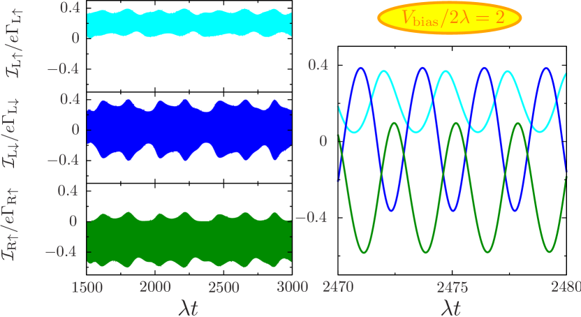
Figure 14: The graphs depict the different contributions to the current in regime III. The right graph presents a detail of the left graphs drawn together for a short time range. Initial conditions and parameters as in Sec. II.2 for regime III.

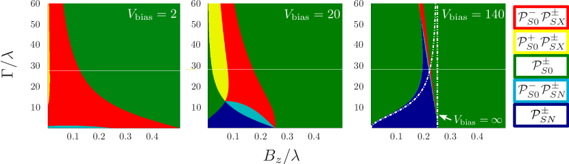
Figure 15: Stable fixed points as a function of tunneling rate and magnetic field. The external bias is increased from left to right, the explicit values are denoted in the graphs (in units of $[\lambda]$). Additionally, the infinite bias result is plotted in the last graph on the right side. The dark blue area denotes the regime where no oscillations appear and only the nodes $\mathcal{P}^{\pm}_{SN}$ exist.

If we decrease the tunneling rate, we observe a transition to chaotic-like oscillations as in the infinite bias case; see Fig. 4. For small values of the bias, the chaotic-like behavior is a little suppressed and the trajectories oscillate comparatively smoothly with a high frequency.

III.2.3 Region III: Oscillations and high frequency

In Sec. II.2 we presented results for larger values of the magnetic field, where the trajectories oscillate around $\mathcal{P}^{\pm}_{S0}$. This kind of behavior is recovered for the finite bias regime. But we observe slight differences in the regime of small bias. In Fig. 14, the current for regime III is depicted ($V_{\rm bias}/2\lambda=2$); the results for the left and the right current are split into their contributions from spin-up and -down electrons. We observe that the current channel $\mathcal{I}_{\rm{L}\downarrow}$ oscillates around the zero axis and, following from that, the current is flowing in both directions. The frequency of the oscillations is quite high, and the spin components oscillate between two cycles, whose signatures are clearly visible in the left graphs of Fig. 14.

IV Conclusion

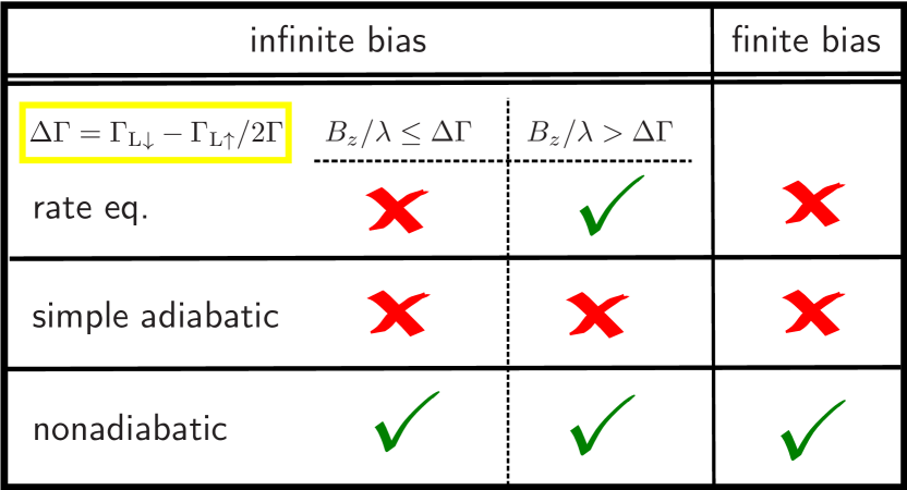
Figure 16: Table listing the regions were the different approaches are valid (green check mark) or not valid (red cross). $\Delta\Gamma$ corresponds to the border between region II and region III, i.e. in our foregoing calculations we had $\Delta\Gamma=1/4$. Note, that this table corresponds to a conservative estimate focusing on parameter regimes where the approaches always coincide with the nonadiabatic approach and for polarized leads.

With our nonadiabatic approach, we are able to probe the rate equation and the adiabatic approach and thus can discuss the advantages and disadvantages of these two methods, cf.Fig. 16.

The rate equation approach from Lopez-Monis2012 , is a quite practical method. The numerical effort is low and the dynamical system can be investigated analytically. However, this method neglects higher-order transitions, and we learned from the nonadiabatic results, that these are relevant in the regime of low magnetic field. In the latter region, the rate equations miss parts of the nonlinear dynamics. If the magnetic field increases, the results of both approaches coincide.

The limitation of the rate equation approach to high external bias is another disadvantage: at finite bias, we observe even richer dynamics within the nonadiabatic approach. There, features such as spin-flips of the large spin and suppression of the oscillations as a function of the applied bias appear. The disadvantages belonging to the nonadiabatic approach are the high numerical effort and its inaccessibility for further analytic investigations.

In our work, we utilized the adiabatic Green’s function method to analyze our system. However, we omitted the presentation of time-dependent results, because this simple adiabatic approach does not capture a lot of the dynamics even in the infinite bias regime. There, the dynamical system reduces to three equations of motion, and only if the trajectories run directly in a stable node and no oscillations appear can the adiabatic approach correctly describe the system.

On the other hand, the adiabatic Green’s functions are suitable for the analysis of the system. For the finite bias regime, our initial adiabatic analysis matched quite well the behavior of the nonadiabatic approach. Therewith, we can re-define the dynamical regions as depicted in Fig. 15. It is clearly visible that the external bias is an important parameter for this system. The regions where only one of the main fixed points $\mathcal{P}^{\pm}_{S0}$ exists are promising for switching of the large spin, but due to the fact that we deal with a multistable system, there are always additional stationary solutions present.

Acknowledgments. This work was supported by projects DFG BR 1528/7-1, DFG BR 1528/8-1, GRK 1558 and the Rosa Luxemburg foundation. We acknowledge fruitful discussions with C. López-Monís, C. Emary, G. Kiesslich and K. Mosshammer.

Appendix A Frequency doubling of $\langle\hat{S}_{z}(t)\rangle$

The equation of motion for the $z$-component of the electronic spin in Eq. (II.2) does not directly couple to the magnetic field, but it couples to the product of the $x$-component for the large spin and the $y$-component of the electronic spin. The latter develop sinusoidally in time with the same frequency $\omega_{s}$ and without a phase shift, cf. Fig. 5. If we approximate their evolution in time with $\langle\hat{J}^{\rm eff}_{x}(t)\rangle=a_{j}\sin{\omega_{s}t}$ and $\langle\hat{S}^{\rm eff}_{y}(t)\rangle=a_{e}\sin{\omega_{s}t}$, we can estimate an effective solution for the $z$-component of the electronic spin ($A_{s}=a_{j}a_{e}$),

$$\langle\hat{S}_{z}^{\rm eff}(t\to\infty)\rangle= \frac{\left(\Gamma_{\rm L\uparrow}-\Gamma_{\rm L\downarrow}+2A_{s}\right)}{2\Gamma}$$

$$-\frac{1}{8}\left[\frac{\cos(2\omega_{s}t)+2\omega_{s}/\Gamma\sin(2\omega_{s}t)}{(\Gamma A_{s})^{-1}(\omega_{s}^{2}-\frac{\Gamma^{2}}{4})}\right].$$ (29)

Hence, the oscillation goes with twice the frequency of the other spin components. Note, that for a more general ansatz, e.g. $\langle\hat{J}^{\rm eff}_{x}(t)\rangle=a_{j}\sin{\omega_{s}t}+b_{j}\cos{\omega_{s}t}$, the result is similar and differs solely in the prefactor.

Appendix B Adiabatic approach: Green’s functions

The expectation values of the spin operators in frequency space are obtained from

$$\langle\hat{S}_{i}(\omega)\rangle=-\frac{i}{2}\ \rm{tr}\left[\textbf{G}^{<}(\omega)\textbf{$\sigma$}_{i}\right],\hskip 14.22636pt\mbox{$i=x,y,z$},$$ (30)

containing the Pauli spin matrices

$$\sigma_{x}=\begin{pmatrix}0&1\\ 1&0\\ \end{pmatrix},\sigma_{y}=\begin{pmatrix}0&-i\\ i&0\\ \end{pmatrix},\sigma_{z}=\begin{pmatrix}1&0\\ 0&-1\\ \end{pmatrix}.$$

If we reconsider the effective Hamiltonian Eq. (II.1) for this system, we recall the similarity to a parallel two-level system, and as in that case, the Green’s functions have matrix character,

$$\textbf{G}(\omega)=\begin{pmatrix}G_{\uparrow\uparrow}(\omega)&G_{\uparrow\downarrow}(\omega)\\ G_{\downarrow\uparrow}(\omega)&G_{\downarrow\downarrow}(\omega)\\ \end{pmatrix}.$$

The off-diagonal functions refer to the coupling to the $x$-component of the large spin. Without this coupling, we end up with two independent levels. For the derivation of the electronic spin we need the lesser Green’s function, whose calculation makes use of the Keldysh equation,

$$G^{<}_{\sigma\sigma^{\prime}}=\sum_{\sigma^{\prime\prime}}\ G^{R}_{\sigma\sigma^{\prime\prime}}(\omega)\ \Sigma^{<}_{\sigma^{\prime\prime}\sigma^{\prime\prime}}(\omega)\ G^{A}_{\sigma^{\prime\prime}\sigma^{\prime}}(\omega),$$ (31)

with the lesser self energy

$$\Sigma^{<}_{\sigma\sigma^{\prime}}(\omega)=\delta_{\sigma,\sigma^{\prime}}\sum_{\alpha}\Sigma^{<}_{\alpha\sigma}=\delta_{\sigma,\sigma^{\prime}}\sum_{\alpha}i\Gamma_{\alpha\sigma}\ f_{\alpha\sigma}(\omega).$$ (32)

The retarded and the advanced Green’s function are obtained from their equation of motion and yield

$$G_{\sigma\sigma}^{R,A}(\omega)= \frac{\omega-\varepsilon_{\sigma^{\prime}}-\Sigma^{R,A}_{\sigma^{\prime}\sigma^{\prime}}}{\left[\omega-\varepsilon_{\sigma}-\Sigma^{R,A}_{\sigma\sigma}\right]\left[\omega-\varepsilon_{\sigma^{\prime}}-\Sigma^{R,A}_{\sigma^{\prime}\sigma^{\prime}}\right]-\frac{\lambda^{2}}{4}\langle\hat{J}_{x}\rangle^{2}},$$

$$G_{\sigma\sigma^{\prime}}^{R,A}(\omega)= \frac{\frac{\lambda}{2}\langle\hat{J}_{x}\rangle}{\omega-\varepsilon_{\sigma}-\Sigma^{R,A}_{\sigma\sigma}}\ G_{\sigma\sigma^{\prime}}(\omega),$$ (33)

with the retarded/advanced self energy

$$\Sigma_{\sigma\sigma^{\prime}}^{R,A}=\delta_{\sigma,\sigma^{\prime}}\sum_{\alpha}\Sigma_{\alpha\sigma}^{R,A}=\delta_{\sigma,\sigma^{\prime}}\sum_{k\alpha}\frac{\left|V_{k\alpha\sigma}\right|^{2}}{\omega-\varepsilon_{k\alpha\sigma}\pm i0},$$ (34)

which real part $\Lambda_{\alpha\sigma}(\omega)$ solely leads to a shift of the level energies $\varepsilon_{d}$ and therefore is neglected. The imaginary part corresponds to the tunneling rate $\Gamma_{\alpha\sigma}(\omega)\equiv\Gamma_{\alpha\sigma}$.

Appendix C Details of the stability analysis

The fixed points of the dynamical system are obtained from Eq. (II), if we set all derivations to zero,

$$0 =-\left(\lambda\langle\hat{S}_{z}\rangle+B_{z}\right)\ \langle\hat{J}_{y}\rangle,$$

$$0 =\hskip 11.38092pt\left(\lambda\langle\hat{S}_{z}\rangle+B_{z}\right)\ \langle\hat{J}_{x}\rangle-\lambda\langle\hat{S}_{x}\rangle\ \langle\hat{J}_{z}\rangle,$$

$$0 =\hskip 14.22636pt\lambda\langle\hat{S}_{x}\rangle\ \langle\hat{J}_{y}\rangle.$$ (35)

This is a strong nonlinear system, because the electronic spin operators depend on the large spin components $\langle\hat{S}_{i}[\langle\hat{J}_{x}\rangle,\langle\hat{J}_{z}\rangle]\rangle$. Here we work in the adiabatic regime where the spin operators are given in terms of Green’s functions, see Eq. (30). The latter contain frequency integrals, leading to expressions with trigonometrical terms. From Eq. (C) an analytic expression for all fixed points is not possible. Instead we obtain transcendental equations which require numerical calculations. This is the case for $\mathcal{P}^{\pm}_{SN}$, where the conditions $\langle\hat{S}_{z}\rangle=-B_{z}/\lambda$ and $\langle\hat{S}_{x}\rangle=0$ have to be fulfilled.

The stability of the stationary solutions obtained from Eq. (C) are investigated with the help of the Jacobian $\mathcal{J}$ of the linearized system. Evaluating this Jacobian at the fixed points provides an answer if a small disturbance from these stationary solutions grows or decays, indicating unstable and stable solutions. Here the Jacobian of the linearized dynamical system yields

$$\mathcal{J}=\begin{pmatrix}-\lambda\frac{\partial\langle\hat{S}_{z}\rangle}{\partial\langle\hat{J}_{x}\rangle}\langle\hat{J}_{y}\rangle&-(\lambda\langle\hat{S}_{z}\rangle+B_{z})&-\lambda\frac{\partial\langle\hat{S}_{z}\rangle}{\partial\langle\hat{J}_{z}\rangle}\langle\hat{J}_{y}\rangle\\[5.69046pt] (\lambda\langle\hat{S}_{z}\rangle+B_{z})+\lambda\frac{\partial\langle\hat{S}_{z}\rangle}{\partial\langle\hat{J}_{x}\rangle}\langle\hat{J}_{x}\rangle-\lambda\frac{\partial\langle\hat{S}_{x}\rangle}{\partial\langle\hat{J}_{x}\rangle}\langle\hat{J}_{z}\rangle&0&-\lambda\langle\hat{S}_{x}\rangle+\lambda\frac{\partial\langle\hat{S}_{z}\rangle}{\partial\langle\hat{J}_{z}\rangle}\langle\hat{J}_{x}\rangle-\lambda\frac{\partial\langle\hat{S}_{x}\rangle}{\partial\langle\hat{J}_{z}\rangle}\langle\hat{J}_{z}\rangle\\[5.69046pt] \lambda\frac{\partial\langle\hat{S}_{x}\rangle}{\partial\langle\hat{J}_{x}\rangle}\langle\hat{J}_{y}\rangle&\lambda\langle\hat{S}_{x}\rangle&\lambda\frac{\partial\langle\hat{S}_{x}\rangle}{\partial\langle\hat{J}_{z}\rangle}\langle\hat{J}_{y}\rangle\\ \end{pmatrix}.$$ (36)

As an example we present the derivation of the fixed points $\mathcal{P}^{\pm}_{S0}$, where the large spin is completely polarized parallel to the magnetic field; cf. Eq. (18). There the $x,y$-components of the electronic spin vanish due to $\langle\hat{J}_{x,0}\rangle=0$. Considering the zero temperature case, where the Fermi function becomes a step function, and with $\varepsilon_{\uparrow,\downarrow}^{\pm}=\varepsilon_{d}\pm 0.5(B_{z}\pm j)$, we obtain for the $z$-component

$$\langle\hat{S}_{z,0}\rangle= \int\frac{d\omega}{4\pi}\sum_{\alpha}\Theta(\mu_{\alpha}-\omega)$$

$$\times\left[\frac{\Gamma_{\alpha\uparrow}}{\left|\left[\omega-\varepsilon_{\uparrow}^{\pm}+i\frac{\Gamma}{2}\right]\right|^{2}}-\frac{\Gamma_{\alpha\downarrow}}{\left|\left[\omega-\varepsilon_{\downarrow}^{\pm}+i\frac{\Gamma}{2}\right]\right|^{2}}\right]$$

$$= \sum_{\alpha}\left\{\frac{\Gamma_{\alpha\uparrow}}{2\pi\Gamma}\arctan\left[\frac{(\mu_{\alpha}-\varepsilon_{\uparrow}^{\pm})}{\Gamma/2}\right]\right.$$

$$\left.\hskip 14.22636pt-\frac{\Gamma_{\alpha\downarrow}}{2\pi\Gamma}\arctan\left[\frac{(\mu_{\alpha}-\varepsilon_{\downarrow}^{\pm})}{\Gamma/2}\right]+\frac{\left(\Gamma_{\alpha\uparrow}-\Gamma_{\alpha\downarrow}\right)}{4\Gamma}\right\}.$$ (37)

Due to $\Gamma=\Gamma_{\sigma\rm{L}}+\Gamma_{\sigma\rm{R}}$ the last term in Eq. (C) vanishes if the summation over $\alpha$ is accomplished and the result Eq. (III.1.1) is obtained.

The Jacobian simplifies to

$$\mathcal{J}^{\pm}_{0}=\begin{pmatrix}0&-(\lambda\langle\hat{S}_{z,0}\rangle+B_{z})&0\\[5.69046pt] \lambda\langle\hat{S}_{z,0}\rangle+B_{z}\mp\left.\lambda j\frac{\partial\langle\hat{S}_{x}\rangle}{\partial\langle\hat{J}_{x}\rangle}\right|_{\begin{subarray}{c}\mathcal{P}^{\pm}_{S0}\end{subarray}}&0&0\\[5.69046pt] 0&0&0\\ \end{pmatrix},$$ (38)

from which the eigenvalues $\mathcal{E}_{2,3}^{0,\pm}$ are calculated, cf. Eq. (III.1.1). The derivation in Eq. (38) is obtained from

$$\left.\frac{\partial\langle\hat{S}_{x}\rangle}{\partial\langle\hat{J}_{x}\rangle}\right|_{\begin{subarray}{c}\mathcal{P}^{\pm}_{S0}\end{subarray}}= \ \lambda\int\frac{d\omega}{4\pi}\sum_{\alpha}\Theta(\mu_{\alpha}-\omega)$$

$$\times\frac{\left[(\omega-\varepsilon_{\downarrow}^{\pm})\Gamma_{\alpha\uparrow}+(\omega-\varepsilon_{\uparrow}^{\pm})\Gamma_{\alpha\downarrow}\right]}{\left|\left[\omega-\varepsilon_{\uparrow}^{\pm}+i\frac{\Gamma}{2}\right]\left[\omega-\varepsilon_{\downarrow}^{\pm}+i\frac{\Gamma}{2}\right]\right|^{2}}.$$ (39)

References

- (1) R. Hanson, L. P. Kouwenhoven, J. R. Petta, S. Tarucha, and L. M. K. Vandersypen, Rev. Mod. Phys. 79, 1217 (2007).
- (2) S. I. Erlingsson, O. N. Jouravlev, and Y. V. Nazarov, Phys. Rev. B 72, 033301 (2005).
- (3) J. Baugh, Y. Kitamura, K. Ono, and S. Tarucha, Phys. Rev. Lett. 99, 096804 (2007).
- (4) K. Ono and S. Tarucha, Phys. Rev. Lett. 92, 256803 (2004).
- (5) S. Takahashi et al., Phys. Rev. Lett. 104, 246801 (2010).
- (6) K. Hamaya et al., Phys. Rev. B 77, 081302 (2008).
- (7) J. R. Hauptmann, J. Paaske, and P. E. Lindelof, Nat Phys 4, 373 (2008).
- (8) M.-H. Jo et al., Nano Letters 6, 2014 (2006).
- (9) H. B. Heersche et al., Phys. Rev. Lett. 96, 206801 (2006).
- (10) L. Bogani and W. Wernsdorfer, Nat Mater 7, 179 (2008).
- (11) M. Misiorny, I. Weymann, and J. Barnaś, Phys. Rev. B 79, 224420 (2009).
- (12) J. R. Friedman and M. P. Sarachik, Annual Review of Condensed Matter Physics 1, 109 (2010).
- (13) N. Bode, L. Arrachea, G. S. Lozano, T. S. Nunner, and F. von Oppen, Phys. Rev. B 85, 115440 (2012).
- (14) L. Thomas et al., Nature 383, 145 (1996).
- (15) M. Feingold and A. Peres, Physica D: Nonlinear Phenomena 9, 433 (1983).
- (16) A. Peres, Phys. Rev. A 30, 504 (1984).
- (17) M. Feingold, N. Moiseyev, and A. Peres, Phys. Rev. A 30, 509 (1984).
- (18) D. T. Robb and L. E. Reichl, Phys. Rev. E 57, 2458 (1998).
- (19) C. López-Monís, C. Emary, G. Kiesslich, G. Platero, and T. Brandes, Phys. Rev. B 85, 045301 (2012).
- (20) A. Metelmann and T. Brandes, Phys. Rev. B 84, 155455 (2011).
- (21) M. J. A. Schuetz, E. M. Kessler, J. I. Cirac, and G. Giedke, Phys. Rev. B 86, 085322 (2012).
- (22) K. Mosshammer, G. Kiesslich, and T. Brandes, Phys. Rev. B 86, 165447 (2012).
- (23) S. Morrison and A. S. Parkins, Phys. Rev. A 77, 043810 (2008).
- (24) S. Morrison and A. S. Parkins, Phys. Rev. Lett. 100, 040403 (2008).
- (25) P. Ribeiro, J. Vidal, and R. Mosseri, Phys. Rev. E 78, 021106 (2008).
- (26) M. S. Rudner and L. S. Levitov, Phys. Rev. B 82, 155418 (2010).
- (27) P. W. Anderson, Phys. Rev. 124, 41 (1961).
- (28) U. Fano, Phys. Rev. 124, 1866 (1961).
- (29) P. Zeeman, Nature 55, 347 (1897).
- (30) L. Hofstetter et al., Phys. Rev. Lett. 104, 246804 (2010).
- (31) B. Sothmann and J. König, Phys. Rev. B 82, 245319 (2010).
- (32) I. Weymann, J. König, J. Martinek, J. Barnaś, and G. Schön, Phys. Rev. B 72, 115334 (2005).
- (33) C. Slicher, Principles of Magnetic Resonance, Springer Berlin, 3 edition, 1990.
- (34) V. Cerletti, W. A. Coish, O. Gywat, and D. Loss, Nanotechnology 16, R27 (2005).
- (35) W. A. Coish and J. Baugh, physica status solidi (b) 246, 2203 (2009).
- (36) J. Fischer, B. Trauzettel, and D. Loss, Phys. Rev. B 80, 155401 (2009).
- (37) L. V. Keldysh, Sov. Phys. JETP 20, 1018 (1965).
- (38) A. Kamenev and A. Levchenko, Advances in Physics 58, 197 (2009).
- (39) H. J. Haug and A.-P. Jauho, Quantum Kinetics in Transport and Optics of Semiconductors, Springer–Verlag, Berlin, 2nd revised edition, 2008.
- (40) J. Könemann, R. J. Haug, D. K. Maude, V. I. Fal’ko, and B. L. Altshuler, Phys. Rev. Lett. 94, 226404 (2005).
- (41) L. G. Mourokh, N. J. M. Horing, and A. Y. Smirnov, Phys. Rev. B 66, 085332 (2002).
- (42) T. Brandes, Physics Reports 408, 315 (2005).
- (43) D. Ralph and M. Stiles, Journal of Magnetism and Magnetic Materials 320, 1190 (2008).
- (44) S. Strogatz, Nonlinear Dynamics and Chaos: With Applications to Physics, Biology, Chemistry and Engineering, Westview, Cambridge, Massachusetts, 3 edition, 2000.
- (45) R. Hussein, A. Metelmann, P. Zedler, and T. Brandes, Phys. Rev. B 82, 165406 (2010).
- (46) Y. A. Kuznetsov, Elements of Applied Bifurcation Theory, volume 112 of Applied Mathematical Science, Springer, New York, 2004.
- (47) A. Beuter, L. Glass, M. C. Mackey, and M. Titcombe, Nonlinear Dynamics in Physiology and Medicine, Springer, New York, 2003.