A class of multi-phase traffic theories for microscopic, kinetic and continuum traffic models

Abstract.

In the present paper a review and numerical comparison of a special class of multi-phase traffic theories based on microscopic, kinetic and macroscopic traffic models is given. Macroscopic traffic equations with multi-valued fundamental diagrams are derived from different microscopic and kinetic models. Numerical experiments show similarities and differences of the models, in particular, for the appearance and structure of stop and go waves for highway traffic in dense situations. For all models, but one, phase transitions can appear near bottlenecks depending on the local density and velocity of the flow.

1. Introduction

Traffic flow modeling has been considered on different levels of description, see [5] for a recent review: on the microscopic level the motion of each vehicle is described. Mathematical models are generally stated using a large system of ordinary differential equations for position and velocity of the vehicles based on Newtonian mechanics [11, 41, 3, 20, 30]. On the macroscopic level the state of the system is described by averaged quantities. Typically, density and linear momentum are used to describe the flow. The corresponding mathematical models are based on systems of nonlinear partial differential equations derived from conservation laws with suitable closure relations. Starting from the pioneering work of Aw and Rascle [2] new macroscopic models for traffic flow have been derived and investigated intensively in the last decade, see for example [7, 14, 1, 23, 21, 28]. These models avoid several inconsistencies of previous models, like wrong way traffic and missing bounds on the density. We note that these models can be derived from microscopic models in a variety of ways, see for example [1, 52]. Finally, kinetic theory describes the state of the system by a probability distribution function of the position and velocity of the vehicles. Mathematical models generally use integro-differential or Fokker-Planck type equations. Kinetic equations for vehicular traffic can be found, for example, in [45, 44, 42, 38]. Procedures to derive macroscopic traffic equations including the Aw/Rascle model from underlying kinetic models have been performed in different ways by several authors, see, for example, [27] and [39]. These procedures are developed in analogy to the transition from the kinetic theory of gases to continuum gas dynamics.

Another basic problem of macroscopic traffic flow equations has been described by Kerner [33, 34, 35]. The observations there suggest a more complicated dependence of the homogeneous steady speed states on density: these states are not given by a uniquely defined function $u=U^{e}(\rho)$ as in the above mentioned models, but cover a whole range in the density-flow diagram leading to a multi-valued fundamental diagram. The resulting dynamical system has a multi-phase behavior in the sense of Kerner: the flow changes between different stationary state which represent free and so called synchronized or jam behavior. In the context of the derivation of macroscopic models from microscopic ones the homogeneous steady state solutions can be interpreted as an emergent behavior of interactions at the microscopic scale and multiple solutions may be related to the heterogeneous behavior of the driver-vehicle subsystem. A variety of microscopic and macroscopic multiphase models has been developed by several authors. In particular, there is a large number of works on microsopic models. We refer among many others to [36, 37, 46, 47, 50, 53, 10, 51]. Macroscopic models for traffic flow with phase transitions in the sense of Kerner can be found in [9, 21, 13, 12]. However, these models do not describe phenomena like stop and go waves near bottlenecks. For microscopic and macroscopic multiphase models exhibiting stop and go waves and similar traffic instabilities we refer to [36, 37, 53, 40, 25, 48]. Kinetic models allowing for multiple stationary solutions and associated macroscopic models with multi-valued fundamental diagrams have been developed in [29, 32, 26, 43]. We refer to [5] for a recent review and to [17, 4, 16] for further material on the above issues.

The present paper contains a comparison and discussion of a class of macroscopic models with multi-valued fundamental diagrams. We consider models of the form

(1) $$\partial_{t}\rho+\partial_{x}(\rho u) = 0,$$

$$\partial_{t}(\rho u)+\partial_{x}(\rho u^{2})-c(\rho)\partial_{x}u = \rho R(u,\tau)$$

with right hand side

$$R(\rho,u)=\;\frac{\rho}{T}\;\left[U(\rho,u)-u\right]$$

and fundamental diagrams given by functions $U=U(\rho,u)$ having at least two equilibrium solutions, i.e. solutions of the equation $u=U(\rho,u)$ for fixed $\rho$ out of a certain density domain, where multiphase traffic may appear.

The paper starts with a review of this class of macroscopic multi-phase models. The models are derived from either microscopic or kinetic equations. To guarantee a proper comparison of the considered models several changes to the original models are proposed. Moreover, the parameters of the different models are chosen such that the stable equilibrium solutions are the same for all models. Then, the different models are numerically investigated for a bottleneck problem and the appearance of stable wave patterns is shown which can be interpreted as stop-and go waves at (on ramp) bottlenecks. This numerical comparison as well as the changes made for each of the models to make them comparable are new up to the knowledge of the authors. We note that stable periodic waves excited by small periodic perturbations have been studied in a series of papers also for equations with single valued right hand sides, see [24, 25, 19]. Remarks on these waves can be found in section 5.

The paper is arranged in the following way: In Section 2 the derivation of macroscopic equations from microscopic models is reviewed and applied to a multi-phase traffic model from [35, 36]. In Section 3 kinetic equations are investigated and used to derive multi-valued fundamental diagrams. The different models are partially changed to make them comparable to each other. Section 4 contains a summary and comparison of the different approaches and the derived multi-valued fundamental diagrams. Finally, in Section 5 numerical results are given comparing the different density-velocity relations. Moreover, an inhomogeneous traffic flow situation with a bottleneck is investigated, showing the appearance of traffic instabilities together with a qualitative comparison of the structure of these instabilities.

2. Continuum multi-phase traffic model derived from microscopic equations

2.1. From microscopic to macroscopic models

We review the classical procedure for so called ’General Motors’ (GM) type car-following models, see [11, 41]. Denoting with $x_{i}(t),v_{i}(t),i=1,\ldots,N$ the location and speed of the vehicles at time $t\in{}^{+}$, and the distance between successive cars by

$$l_{i} = x_{i+1}-x_{i},$$

we consider the microscopic equations

$$\dot{x}_{i} = v_{i}$$

$$\dot{v}_{i} = C\frac{(v_{i+1}-v_{i})}{l_{i}-H}+\frac{1}{T}(U(\rho_{i})-v_{i}).$$

The local “density around vehicle i” and its inverse (the local (normalized) “specific volume”) are respectively defined by

$$\rho_{i}=\frac{H}{l_{i}}\;\mbox{and}\;\;\tau_{i}=\frac{1}{\rho_{i}}=\frac{l_{i}}{H},$$

where $H$ is the length of a car.

Remark 2.1.

Here, the density is normalized and therefore dimensionless, so that the maximal density is $\rho_{m}=1/\tau_{m}=1$.

The constant $C>0$ and the relaxation time $T$ are given parameters. The function $U=U(\rho),0\leq\rho\leq\rho_{m}=1$ is the so called fundamental diagram, see [45, 37, 48]. The simplest choice is given by $U(\rho)=1-\rho$. One obtains the microscopic model

(2) $$\dot{x}_{i} = v_{i}\;,$$

$$\dot{v}_{i} = \frac{C}{H}\;\frac{(v_{i+1}-v_{i})}{\tau_{i}-1}+\;\frac{1}{T}\left(U(\rho_{i})-v_{i}\right).$$

We have

$$\dot{l}_{i}=v_{i+1}-v_{i}\;\;\mbox{or}\;\;\dot{\tau}_{i}=\frac{1}{H}\;(v_{i+1}-v_{i}).$$

The limit of number of cars going to infinity yields the Lagrangian form of the macroscopic equations, see [1]. We obtain the equivalent of the p-system in gas dynamics (isentropic Euler equations in Lagrangian form), compare [22],

(3) $$\partial_{T}\tau-\partial_{X}u = 0\;,$$

$$\partial_{T}u-c(\rho)\partial_{X}u = \;\frac{1}{T}\left[U(\rho)-u\right]\;,$$

where $\tau=\frac{1}{\rho}$ is the specific volume, i.e. the (local) dimensionless fraction of space occupied by the cars. $\rho$ the (normalized) density is the limit of $\rho_{i}$ defined above, as the number of cars tends to infinity. $u$ is the macroscopic velocity of the cars. Moreover,

(4) $$c(\rho)=C\left(\frac{1}{\rho}-1\right)^{-1}$$

and the function $U(\rho)$ is defined in the microscopic model above. We change the Lagrangian “mass” coordinates $(X,T)$ into Eulerian coordinates $(x,t)$ with

$$\partial_{x}X=\rho,\;\partial_{t}X=-\rho v,\;T=t$$

or

$$\partial_{X}x=\rho^{-1}=\tau,\;\partial_{T}x=v.$$

Thus, $X=\int^{x}\rho(y,t)dy$ describes the total space occupied by cars up to point $x$. The macroscopic system in Eulerian coordinates is then

(5) $$\partial_{t}\rho+\partial_{x}(\rho u) = 0,$$

$$\partial_{t}(\rho u)+\partial_{x}(\rho u^{2})-c(\rho)\partial_{x}u = \;\frac{\rho}{T}\;\left[U(\rho)-u\right].$$

For the well-posedness of the above problem we refer to [8].

Remark 2.2.

The same approach works for right hand sides with multi-valued equilibrium distributions

(6) $$\;\frac{\rho}{T}\;\left[U(\rho,u)-u\right].$$

Examples are Switching curve (SC) models as in [25] with

$$U(\rho,u)=\begin{cases}U_{1}(\rho),&\rho<\rho_{f}\;\mbox{or}\;u>S(\rho),\rho_{f}<\rho<\rho_{j},\\ U_{2}(\rho),&u<S(\rho),\rho_{f}<\rho<\rho_{j}\mbox{or}\;\rho>\rho_{j}.\end{cases}$$

Here the switching curve $S=S(\rho)$ is given. We consider the density in the (synchronized flow) region between a lower bound of free flow $\rho_{f}$ and an upper bound of jam traffic $\rho_{j}$. Then, there exists multiple stationary states $U_{1},U_{2}$ whose regions of influence are separated by the switch-curve $S$.

A similar model is the Speed-adaptation (SA) type models of Kerner et.al [36] with

$$U(\rho,u)=\begin{cases}U_{1}(\rho),&u>U_{sync},\rho<\rho_{j},\\ U_{2}(\rho),&u<U_{sync},\rho>\rho_{f},\\ \end{cases}$$

where the parameter $U_{syn}$ is the averaged speed, which separates the domains of influence of the two stationary states in the 2-D region of synchronized flow in the flow-density plane.

2.2. A microscopic ATD-type model

In this section we sketch a simplified version of the microscopic Acceleration time delay (ATD) model of Kerner et. al [36]. We consider a microscopic model with the variables space, velocity and acceleration:

(7) $$\dot{x}_{i} = v_{i}$$

$$\dot{v}_{i} = a_{i}$$

$$\dot{a}_{i} = F(a_{i},v_{i},\frac{v_{i+1}-v_{i}}{H},\frac{x_{i+1}-x_{i}}{H})$$

with

$$F(a_{i},v_{i},\frac{\Delta v_{i}}{H},\tau_{i})=\begin{cases}(a_{i}^{free}-a_{i})/T_{del},&\tau_{i}>G(v_{i}),\tau_{i}>\tau_{jam},\\ (a_{i}^{syn}-a_{i})/T_{del},&\tau_{i}<G(v_{i}),\tau_{i}>\tau_{jam},\\ (a_{i}^{jam}-a_{i})/T_{del},&\tau_{i}<\tau_{jam}.\\ \end{cases}$$

Here, $\Delta v_{i}=v_{i+1}-v_{i}$ and $a_{i}^{free},a_{i}^{syn},a_{i}^{jam}$ denote the desired accelerations in the free, synchronized and jam region respectively and $T_{del}$ denotes the time delay of the acceleration of the vehicle. The function $G$ separates the free from the synchronized acceleration behaviour and will be fixed later at the end of Section 4. For a proper comparison with the above models we change the definitions in[36] of the different accelerations slightly and define the terms as follows

$$a_{i}^{free} = \frac{1}{T}(U(\rho_{i})-v_{i})+\frac{c(\rho_{i})}{H}\Delta v_{i}$$

$$a_{i}^{syn} = \frac{1}{T}\min(U(\rho_{i})-v_{i},0)+\frac{c(\rho_{i})}{H}\Delta v_{i}$$

$$a_{i}^{jam} = -\frac{1}{T}v_{i}+\frac{c(\rho_{i})}{H}\Delta v_{i},$$

where $U(\rho)$ and $c(\rho)$ are given as before. This means acceleration depends on the speed difference to the predecessor and a term relaxing to a desired acceleration.

The hydrodynamic multi-phase model

To obtain the hydrodynamic version of the microscopic model in the last section we follow the procedure in Section 2.1. In Lagrangian coordinates we obtain directly

(8) $$\partial_{T}\tau-\partial_{X}u = 0\;,$$

$$\partial_{T}u = a$$

$$\partial_{T}a = F(a,u,\partial_{X}u,\tau).$$

This leads to the following equations in Eulerian coordinates

(9) $$\partial_{t}\rho+\partial_{x}(\rho u) = 0,$$

$$\partial_{t}(\rho u)+\partial_{x}(\rho u^{2}) = \rho a$$

$$\partial_{t}(\rho a)+\partial_{x}(\rho ua) = \rho F(a,u,\tau\partial_{x}u,\tau).$$

A reduced model

Assuming that the delay times for acceleration are small we can reduce the above ATD-type model to

(10) $$\partial_{t}\rho+\partial_{x}(\rho u) = 0,$$

$$\partial_{t}(\rho u)+\partial_{x}(\rho u^{2})-c(\rho)\partial_{x}u = \rho R(u,\tau),$$

where

$$R(\rho,u)=\begin{cases}\frac{1}{T}(U(\rho)-u),&\tau>G(u),\tau>\tau_{j},\\ \frac{1}{T}\min(U(\rho)-u,0),&\tau<G(u),\tau>\tau_{j},\\ -\frac{1}{T}u,&\tau<\tau_{j}.\\ \end{cases}.$$

This is equivalent to

$$R(\rho,u)=\;\frac{\rho}{T}\;\left[U(\rho,u)-u\right]$$

with

$$U(\rho,u)=\begin{cases}U(\rho),&\tau>G(u),\rho<\rho_{j}\;\mbox{or }\;\tau<G(u),u>U(\rho),\rho<\rho_{j},\\ u,&\tau<G(u),u<U(\rho),\rho<\rho_{j},\\ 0,&\rho>\rho_{j}.\\ \end{cases}$$

For comparison with the other multi-valued fundamental diagrams we rewrite the relaxation term using $K(u)=1/G(u)$:

$$U(\rho,u)=\begin{cases}U(\rho),&\;\rho<K(u),\rho<\rho_{j}\;\mbox{or }\;\rho>K(u),u>U(\rho),\rho_{f}<\rho<\rho_{j},\\ u,&\rho>K(u),u<U(\rho),\rho_{f}<\rho<\rho_{j},\\ 0,&\rho>\rho_{j}.\\ \end{cases}$$

3. Multi-phase hydrodynamic equations derived from kinetic equations

3.1. Kinetic equations and correlations

The basic quantity in a kinetic approach is the single car distribution $f(x,v)$ describing the density of cars at $x$ with velocity $v$. The total density $\rho$ on the highway is

$$\rho(x)\;=\;\int_{0}^{w}f(x,v)dv,$$

where $w$ denotes the maximal velocity. Let $F(x,v)$ denote the probability distribution in $v$ of cars at $x$, i.e. $f(x,v)=\rho(x)F(x,v)$. The mean velocity is

$$u(x)\;=\;\int_{0}^{w}vF(x,v)dv.$$

An important role is played by the distribution $f^{(2)}(x,v,h,v_{+})$ of pairs of cars being at the spatial point $x$ with velocity $v$ and leading cars at $x+h$ with velocity $v_{+}$. This distribution function has to be approximated by the one-vehicle distribution function $f(x,v)$. We use the chaos assumption

$$f^{(2)}(x,v,h,v_{+})=q(h)\,f(x,v)\,F(x+h,v_{+}),$$

compare [42]. For a vehicle with velocity $v$ the function $q(h,v;\rho,u)$ denotes the distribution of leading vehicles with distance $h$ under the assumption that the velocities of the vehicles are distributed according to the distribution function $f$.

Thresholds for braking ($H_{B}$) and acceleration ($H_{A}$) are introduced. From a microscopic point of view drivers will brake, once the distance between the driver and its leading car is becoming smaller than a threshold $H_{B}$ and will accelerate, once this distance is becoming larger than $H_{A}$. Otherwise the cars will not change the velocities. Velocities are changed instantaneously once acceleration or braking lines are reached. Models including acceleration of the cars can be developed as well, see [32] for an example.

The distribution of leading vehicles $q(h)$ is prescribed a priori. The main properties, which $q(h)$ has to fulfill are positivity,

$$\int_{0}^{\infty}q(h)dh\;=\;1,$$

and

(11) $$\int_{0}^{\infty}hq(h)dh\;=\;\frac{1}{\rho}.$$

Equation (11) means that the average headway of the cars is $1/\rho$. The leading vehicles are assumed to be distributed in an uncorrelated way with a minimal distance $H_{B}$ from the car under consideration, see [42]:

$$q(h)\;=\;\tilde{\rho}\,e^{-\tilde{\rho}(h-H_{B})}\,\chi_{[H_{B},\infty)}(h).$$

The reduced density $\tilde{\rho}$ has to be defined in such a way, that (11) is fulfilled. One obtains

(12) $$\tilde{\rho}\;=\;=\;\frac{\rho}{1-\rho\,H_{B}}.$$

We note that

$$q_{A}=q(H_{A})\;=\;\tilde{\rho}\,e^{-\tilde{\rho}(H_{A}-H_{B})}$$

and

$$q_{B}=q(H_{B})\;=\;\tilde{\rho}\;.$$

The probability $P_{ov}=P_{ov}(\rho,u)$ for overtaking or lane changing and the corresponding probability $P_{B}=1-P_{ov}$ for braking are determined from phenomenological considerations: at constant density, free flow of cars, i.e. larger velocities will be related to larger probabilites of overtaking or smaller probabilites of braking. So called synchronized traffic is associated to smaller velocities and thus larger probabilites of braking. That means the probablitiy of braking can be considered as - for fixed density – a decaying function of velocity $u$. Similar arguments can be found for example in [35].

Remark 3.1.

In the following we present a kinetic model. Note that the results like multi-valued fundamental diagrams and stop and go behaviour of the derived macroscopic equations do not depend on the exact choice of the microscopic interactions we have chosen here. The model discussed in the next section is only chosen due to the fact that explicit stationary solutions are available. We could as well have chosen models like in [39] or Fokker-Planck type models like in [32].

3.2. The evolution equation

To write the kinetic evolution equations in a simple form we use

$$k\;=\;k(\rho,u)\;=\;\frac{P_{B}\,q_{B}}{q_{A}+P_{B}q_{B}}$$

and

$$\gamma\;=\;\gamma(\rho,u)\;=\;\frac{q_{A}}{1-k}\;=\;q_{A}+P_{B}q_{B}.$$

We consider a relaxation frequency

$$\nu\;=\;\nu(k)$$

and define

$$\frac{1}{T}=\gamma\,\nu.$$

The kinetic model is then given by the following evolution equation for the distribution function $f$:

$$\partial_{t}f+v\partial_{x}f = C^{+}(f)$$

$$= \gamma\Big{[}k(G^{+}_{B}-L^{+}_{B})(f)+(1-k)(G^{+}_{A}-L^{+}_{A})(f)$$

$$+\nu(G_{S}-L_{S})(f)\Big{]}$$

with the loss and gain terms for braking interactions

$$G_{B}^{+}(f) = \int\int_{\hat{v}>\hat{v}_{+}}|\hat{v}-\hat{v}_{+}|\sigma_{B}(v;\hat{v},\hat{v}_{+})f(x,\hat{v})F(x+H_{B},\hat{v}_{+})d\hat{v}d\hat{v}_{+}$$

$$L_{B}^{+}(f) = \int_{\hat{v}_{+}<v}|v-\hat{v}_{+}|f(x,v)F(x+H_{B},\hat{v}_{+})d\hat{v}_{+}.$$

The loss and gain terms for acceleration is defined as

$$G_{A}^{+}(f) = \int\int_{\hat{v}<\hat{v}_{+}}|\hat{v}-\hat{v}_{+}|\sigma_{A}(v;\hat{v},\hat{v}_{+})f(x,\hat{v})F(x+H_{A},\hat{v}_{+})d\hat{v}d\hat{v}_{+}$$

$$L_{A}^{+}(f) = \int_{\hat{v}_{+}>v}|v-\hat{v}_{+}|f(x,v)F(x+H_{A},\hat{v}_{+})d\hat{v}_{+}.$$

Finally terms describing the random behavior of drivers are

$$G_{S}(f) = \int_{0}^{w}\sigma_{S}(v,\hat{v})f(x,\hat{v})d\hat{v}$$

$$\vphantom{\int_{0}^{w}}L_{S}(f) = f(v).$$

$\sigma_{B}$ and $\sigma_{A}$ denote the distribution of the new velocities $v$ after an interaction. Reaching the braking line the vehicle brakes, such that the new velocity $v$ is distributed with a distribution function $\sigma_{B}$ depending on the old velocities $\hat{v},\hat{v}_{+}$. For acceleration the new velocity is distributed according to $\sigma_{A}$. The relaxation term is introduced to include a random behaviour of the drivers.

Remark 3.2.

For further details on this Boltzmann/Enskog approach to traffic flow modelling see [38].

Example

For the probability distributions $\sigma_{A},\sigma_{B}$ we choose the following simple expressions:

(14) $$\sigma_{B}(v,\hat{v},\hat{v}_{+})\;=\;\frac{1}{\hat{v}-\hat{v}_{+}}\,\chi_{[\hat{v}_{+},\hat{v}]}(v)$$

and

(15) $$\sigma_{A}(v,\hat{v},\hat{v}_{+})\;=\;\frac{1}{\hat{v}_{+}-\hat{v}}\,\chi_{[\hat{v},\hat{v}_{+}]}(v).$$

This means we have an equidistribution of the new velocities between the velocity of the car and the velocity of its leading car. Finally,

(16) $$\sigma_{S}(v,\hat{v})\;=\;\frac{1}{w}.$$

3.3. Stationary Distributions and multi-valued Fundamental Diagrams

In this section we investigate the stationary homogeneous equations and determine the multi-valued fundamental diagrams. We consider the local interaction operator:

$$C(f)\;=\;\gamma\left[k(G_{B}-L_{B})(f)+(1-k)(G_{A}-L_{A})(f)+\nu(G_{S}-L_{S})(f)\right]$$

with $f=\rho F$. The gain and loss terms $G_{B},L_{B}$, etc. are defined in the same way as $G_{B}^{+},L_{B}^{+}$, etc., except that $x+H_{X},X=A,B$ is substituted by $x$, wherever it appears. The homogeneous stationary equation is

$$C(f)\;=\;0.$$

We assume that for fixed $\rho$ and $k$ there is a unique solution

$$f\;=\;f^{e}\;=\;\rho F^{e}(k,v)$$

of this equation. This is true for the example stated above.

Thus, for fixed $k$ the mean value of $F^{e}$ is then

$$u^{e}(k)\;:=\;\int_{0}^{w}vF^{e}(k,v)dv.$$

The function $u^{e}$ is uniquely determined due to the above assumption as a function of $k$. However, this does not yield immediately the fundamental diagram, i.e. an equilibrium relation between flux and density.

Instead, the fundamental diagram is determined from the following considerations: let $u$ be the (possibly multi-valued) solution of the equation

(17) $$u \;=\;u^{e}(k(\rho,u))$$

for fixed $\rho$. If there is a unique solution we obtain a well defined relation for equilibrium velocity and density and the usual fundamental diagram. However, in general this equation will have a multitude of different solutions $u$, even infinitely many. Plotting a dependence of this solution on the density one obtains in the general case a two-dimensional region in the density-velocity plane, where the solutions are located. The fundamental diagram is then a multi-valued function.

Remark 3.3.

For the example above the homogeneous solution can be solved explicitly and the corresponding multi-valued solutions of equation (17) can be evaluated numerically. Explicit expressions for $F^{e}(k)$ and $u^{e}(k)$ can be found in [26]. A plot of $u^{e}(k)$ is shown in Figure 2.

Remark 3.4.

In contrast to the other models described above the kinetic approach gives an explanation for a multi-valued fundamental diagram using in particular the braking probability $P_{B}$ as a basic quantity.

3.4. Derivation of Macroscopic Models

In this section macroscopic equations for density and mean velocity are derived. Different procedures are described, for example in [39, 31].

Balance Equations

Multiplying the inhomogeneous kinetic equation (3.2) with $1$ and $v$ and integrating it with respect to $v$ one obtains the following set of balance equations:

(18) $$\partial_{t}\rho+\partial_{x}(\rho u) = 0$$

$$\partial_{t}(\rho u)+\partial_{x}(P+\rho u^{2})+E = S$$

with the ’traffic pressure’

(19) $$P\;=\;\int_{0}^{w}(v-u)^{2}fdv,$$

the Enskog flux term

(20) $$E\;=\;\int_{0}^{w}v[C(f)(x,v,t)-C^{+}(f)(x,v,t)]dv,$$

and the source term

(21) $$S\;=\;\int_{0}^{w}vC(f)(x,v,t)dv.$$

For the present discussion we are, in particular, interested in the source term S.

Closure

We concentrate on the relaxation term and cite the results for the other terms , compare [39]. The traffic pressure $P$ is negligible and approximated by zero, see [39]. Moreover, the Enskog term $E$ is approximated by linearizing expression (20) for $E$ in $H$. We obtain [39]

$$E\;\sim\;-c_{kin}(\rho)\partial_{x}u$$

with $c_{kin}(\rho)$ given by the details of the collision operator. In the following we will neglect the special form of $c_{kin}$ and choose $c_{kin}=c(\rho)$ for comparison as in the other models described above.

Finally, the source term $S$ has to be approximated. We use a relaxation time approximation

$$C(f)\;\sim\;\frac{1}{T}\left(f^{e}(k(\rho,u),v)-f(v)\right).$$

This yields

$$S\;\sim\;S^{e}(\rho,u)\;=\;\rho\frac{1}{T}\left(u^{e}(k(\rho,u))-u\right).$$

Thus, from the kinetic approach one obtains macroscopic equations of the form

(22) $$\partial_{t}\rho+\partial_{x}(\rho u) = 0$$

$$\partial_{t}(\rho u)+\partial_{x}(\rho u^{2})-c(\rho)\partial_{x}u = S^{e}(\rho,u)$$

with

$$S^{e}(\rho,u)\;=\;\rho\frac{1}{T}\left(u^{e}(k(\rho,u))-u\right),$$

where $k=k(\rho,u)$ is defined as

$$k\;=\;\frac{P_{B}\,q_{B}}{q_{A}+P_{B}q_{B}}=\frac{1}{1+\frac{\mbox{exp}(-\tilde{\rho}(H_{A}-H_{B})}{P_{B}}}.$$

Choosing $H_{A}=H_{B}$ this simplifies to

$$k\;=\;\frac{1}{1+\frac{1}{P_{B}}}.$$

Remark 3.5.

One obtains a multi-valued variant of the Aw-Rascle equations with a multi-valued relaxation term on the right hand side.

4. Comparison of multi-phase hydrodynamic models

We consider models of the form

(23) $$\partial_{t}\rho+\partial_{x}(\rho u) = 0,$$

$$\partial_{t}(\rho u)+\partial_{x}(\rho u^{2})-c(\rho)\partial_{x}u = \rho R(u,\tau)$$

with

(24) $$c(\rho)=C\left(\frac{1}{\rho}-1\right)^{-1}$$

and

$$R(\rho,u)=\;\frac{\rho}{T}\;\left[U(\rho,u)-u\right]$$

and fundamental diagrams given by functions $U$ of the following form:

ATD-type models

$$U(\rho,u)=\begin{cases}U(\rho),&\;\rho<K(u),\rho<\rho_{j}\;\mbox{or }\;\rho>K(u),u>U(\rho),\rho_{f}<\rho<\rho_{j},\\ u,&\rho>K(u),u<U(\rho),\rho_{f}<\rho<\rho_{j},\\ 0,&\rho>\rho_{j}.\\ \end{cases}$$

SA-type models

$$U(\rho,u)=\begin{cases}U_{1}(\rho),&u>U_{sync},\rho<\rho_{j},\\ U_{2}(\rho)&u<U_{sync},\rho>\rho_{f},\\ \end{cases}$$

See Kerner et.al. [36] for details.

Switching curve models

$$U(\rho,u)=\begin{cases}U_{1}(\rho),&\rho<\rho_{f}\;\mbox{or}\;u>S(\rho),\rho_{f}<\rho<\rho_{j},\\ U_{2}(\rho),&u<S(\rho),\rho_{f}<\rho<\rho_{j}\;\mbox{or}\;\rho>\rho_{j}.\end{cases}$$

where $S(\rho)$ is a switching curve. For an investigation of these models, see [25].

Kinetic models:

$$U(\rho,u)=u^{e}(k(\rho,u))$$

with

$$k\;=\;\frac{1}{1+\frac{1}{P_{B}}}.$$

In Figure 3 we plot the equilibrium solutions of $u=U(\rho,u)$ together with the values $U(\rho,u)-u$ denoting the length of the arrows. Moreover, $U(\bar{\rho},u)-u$ is plotted for fixed $\rho$ versus $u$ in Figures 7.

For a proper comparison of the above models the parameters are chosen as follows:

$$U(\rho)=U_{1}(\rho)$$

$$K^{-1}(\rho)=U_{2}(\rho),\rho_{j}>\rho>\rho_{f}$$

$$K(u)=\rho_{f},u>U_{2}(\rho_{f})$$

$$U_{2}(\rho)<U_{sync}<U_{1}(\rho),\rho_{f}<\rho<\rho_{j}.$$

Moreover, the functions $\nu$ and $P_{B}$ in the kinetic model are chosen such that the stable kinetic equilibrium solutions of $u=u^{e}(k(\rho,u))$ are given by $U_{1}$ and $U_{2}$, the instable solution by $S(\rho)$. This leads to the fundamental diagrams shown in Figures 3 to 6.

5. Numerical Investigations

In this section we compare the different approaches numerically. First, the kinetic model is investigated and the associated fundamental diagram is determined. Second the other three models stated in the last section are compared to the kinetic approach and third all three approaches are used in a inhomogeneous traffic simulation with a bottleneck.

5.1. The stationary, homogeneous kinetic equation

We consider the kinetic equation and resulting fundamental diagrams. For the numerical simulations we normalize and use $w=1$.

Moreover, we choose $\nu$ as in Figure 1. A reasonable function $\nu$ should be zero for maximal density ($k=1$). In this case there is no more random behaviour of the drivers, all drivers have velocity $0$. For the case $k=0$ we have chosen $\nu$ as a finite quantity. If these two features are fulfilled, the qualitative behaviour of the model does not depend on the exact form of $\nu$. The braking probability $P_{B}$ is plotted as well in Figure 1.

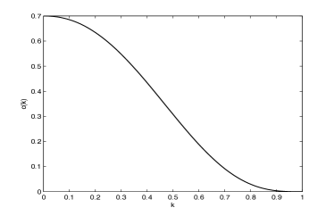
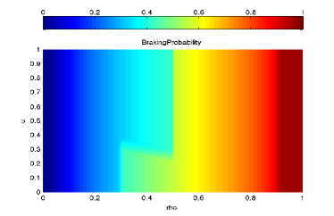
Figure 1. Left: Frequency of random events $\nu(k)$. Right: Braking Probability $P_{B}(\rho,u)$.

Using $P_{B}$ and $\nu$ described above we compute for fixed $k$ the unique stationary solution of the homogeneous kinetic equation and the function $u^{e}(k)$ following Section 3.3. The dependence of $u^{e}$ on $k$ is plotted in Figure 2.

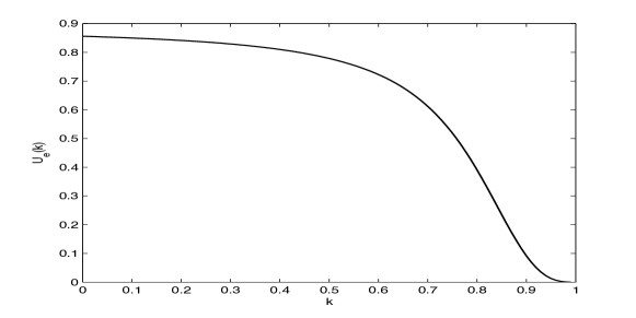
Figure 2. Function $u^{e}(k)$

5.2. The multi-valued fundamental diagrams

In this subsection we plot the multi-valued fundamental diagrams for the four cases discussed in section 4. The functions $U_{1}(\rho)$ and $U_{2}(\rho)$ for ATD and switching curve models were chosen as

$$U_{1}(\rho)\;=U_{0}\mbox{tanh}\left(\frac{C_{U}}{T_{0}U_{0}}\left(\frac{1}{\rho}-0.05\right)\right)$$

$$U_{2}(\rho)\;=U_{0}^{*}\mbox{tanh}\left(\frac{C_{U}}{T_{0}U_{0}^{*}}\left(\frac{1}{\rho}-1.1\right)\right)$$

with $U_{0}=0.85,\;C_{U}=0.45,\;U_{0}^{*}=0.5,\;T_{0}=2.9$. Moreover, $T=5,\;C=0.3,\;U_{sync}=0.28$ and $S=S(\rho)$ is given by a linear function connecting $U_{1}(\rho_{f})$ and $U_{2}(\rho_{j})$. The solutions of the nonlinear equation $u=U(\rho,u)$ are plotted together with a plot of the quantity $U(\rho,u)-u$ as arrows with direction $\pm u$. Figure 3, 4, 5 and 6 show the multi-valued fundamental diagram (speed-density relation) for the different models. In each figure, a zoom of the multi-valued region is shown.

In all cases the values for $\rho_{f}$ and $\rho_{j}$ are chosen as $0.3$ and $0.5$ respectively such that for $\rho<\rho_{f}$ we have only one steady solution. For $\rho_{f}<\rho<\rho_{j}$ three (infinitely many for ATD) solutions exist. And for the region $\rho>\rho_{j}$ again only one solution exists.

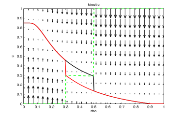
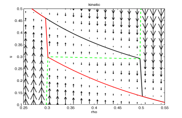
Figure 3. $U(\rho,u)-u$ for the kinetic model. On the Right: a zoom of the multi-valued region.

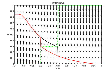
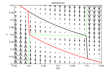
Figure 4. $U(\rho,u)-u$ for the switching curve model. On the Right: a zoom of the multi-valued region.

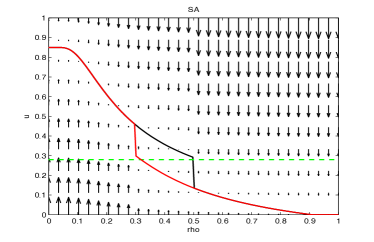
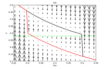
Figure 5. $U(\rho,u)-u$ for the SA model. On the Right: a zoom of the multi-valued region.

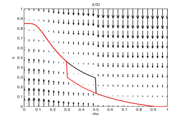
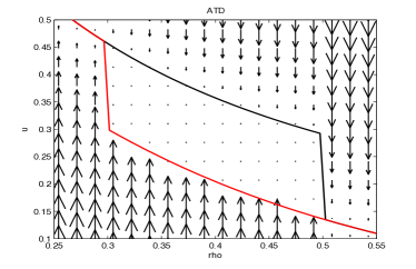
Figure 6. $U(\rho,u)-u$ for the ATD model. On the Right: a zoom of the multi-valued region.

Moreover, Figure 7 shows the values of $U(\rho,u)-u$ for a fixed value $\rho=\bar{\rho}$ with $\rho_{f}<\bar{\rho}<\rho_{j}$.

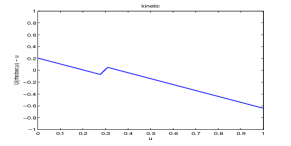
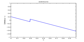
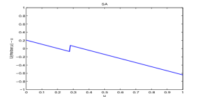
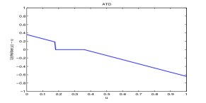
Figure 7. $U(\bar{\rho},u)-u$ for the kinetic, switching curve, SA and ATD models.

5.3. Numerical solution of multi-phase macroscopic equations

Finally, the macroscopic equations are investigated for a bottleneck situation. For the computations we choose a Godunov method, see [49]. We use a mesh size $\Delta x=0.15$, the Courant number $\lambda_{cfl}=0.99$ and a computation time $T_{end}=400$ units. Figures 8, 9, 10 and 11 show the velocity and density in space and time for a three lane highway with a reduction of lanes from $3$ to $2$ at $X=0$ for the four different models. In the simulation, the lane reduction is achieved by multiplying the density $\rho$ in the term on the right hand side of the equations by a factor $\frac{2}{3}$ for $X>0$ units and using a linear interpolation between the 2 regions. Apart from the ATD-type model, one clearly observes large changes in velocity and density in the backwards propagating traffic jams which might be interpreted as stop and go behaviour. Figure 12 show the flow-density relation at various locations of the considered highway, i.e. upstream of the bottleneck ($X=-20$), within the bottleneck ($X=0$),and downstream of the bottleneck ($X=5$). The flow rate drops from the initial value used in the simulation to settle at the maximum values for the considered highway’s downstream location, $X=5$. For the ATD model in its present form we obtain a rather different behavior due to the zero forcing inside the multi-valued region.

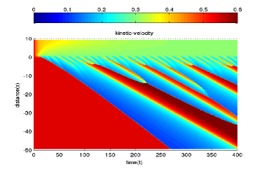
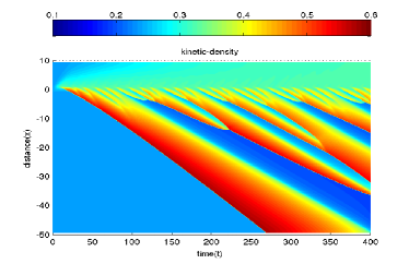
Figure 8. Spatio-temporal congested traffic pattern - velocity(Left) and density(Right) for the kinetic model.

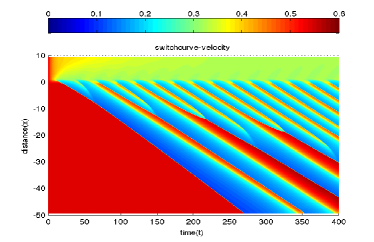
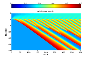
Figure 9. Spatio-temporal congested traffic pattern - velocity(Left) and density(Right) for the switching curve model.

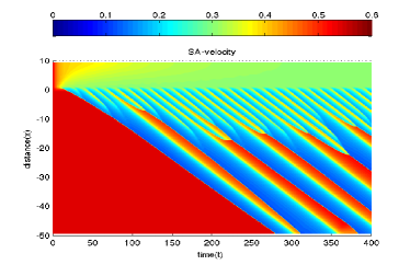
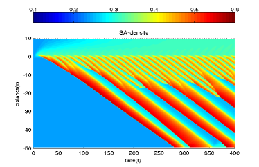
Figure 10. Spatio-temporal congested traffic pattern - velocity(Left) and density(Right) for the SA model.

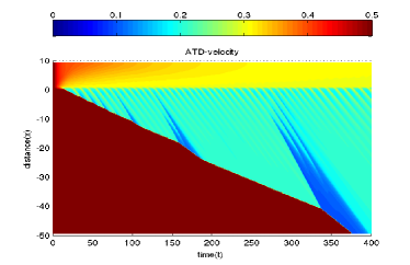
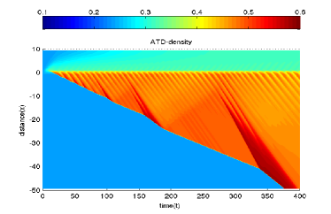
Figure 11. Spatio-temporal congesting traffic pattern - velocity(Left) and density(Right) for the ATD model.

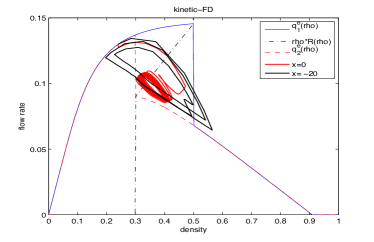
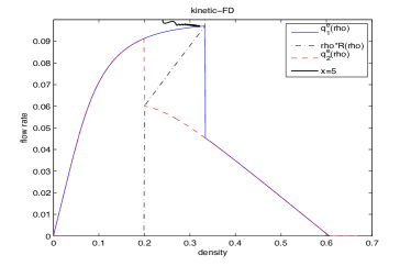
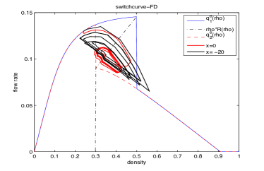
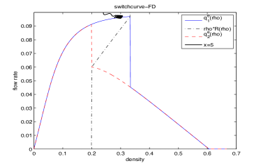
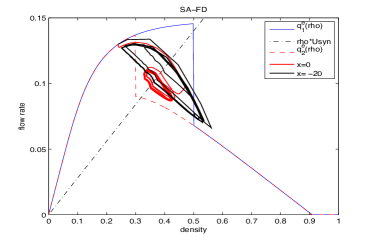
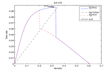
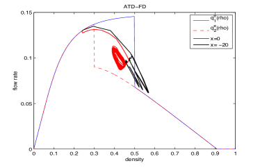
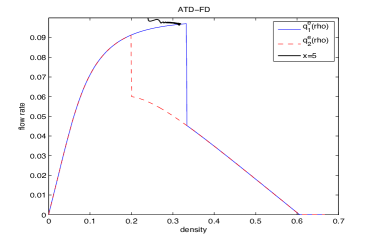
Figure 12. $\rho u-\rho$ relation for the kinetic, switching curve, SA and ATD models upstream ($x=-20$), within ($x=0$) and downstream ($x=5$) of the bottleneck.

Remark 5.1.

The models differ in the frequency and uniformity of the waves generated at the bottleneck. The fact that the ATD model does not generate stable waves in this situation does not mean that the model is in general incapable to describe traffic situation with such patterns. For example, in [36] situations are described where these waves appear. The models derived from the kinetic equations can be viewed as intermediate models between switching curve and ATD model, compare Figure 7.

Remark 5.2.

A similar investigation could be performed for the model in [9, 12] with suitable right hand side.

Remark 5.3.

Using the coefficient $c(\rho)=C\rho$ as done for example in [14], we obtain similar simulation results as above, if the parameters are suitably choosen.

Remark 5.4.

The stable waves excited by small periodic perturbations as discussed in [25, 24] which may also be obtained from equations with single valued right hand sides are usually not persistent anymore for bottleneck situations. These waves are damped out as the high density region travels backward from the bottleneck.

Summary

Multi-valued fundamental diagrams are obtained using different approaches: a derivation from microscopic equations given in [34, 36], from kinetic models as in [26] and a phenomenological macroscopic model from [25]. These approaches are compared with each other from the point of view of their multi-valued fundamental diagrams and for an inhomogeneous bottleneck simulations without any external excitation. Apart from the ATD-type model, all the other models are able to show stop and go patterns for the described situation with a bottleneck without external excitation of waves by the ingoing flow from an on-ramp.

Acknowledgments

The present work has been supported by the DAAD, PhD-Program MIC, Kaiserslautern.

References

- [1] Aw, A., Klar, A., Materne, T., and Rascle, M., Derivation of Continuum Traffic Flow Models from Microscopic Follow-the-Leader Models. SIAM J. Appl. Math. 63 (1) (2002), pp. 259-278.
- [2] A. Aw and M. Rascle, Resurrection of second order models of traffic flow, SIAM J. Appl. Math., 60 (2000), pp. 916-938.
- [3] M. Bando, K. Hasebe, A. Nakayama, A. Shibata, and Y. Sugiyama, Dynamical model of traffic congestion and numerical simulation, Phys. Rev. E, 51 (1995), pp. 1035-1042
- [4] N. Bellomo, M. Delitala, and V. Coscia, On the mathematical theory of vehicular traffic flow and fluid dynamic and kinetic modelling, Math. Models Methods Appl. Sci., 12 (2002), pp. 1801-1843.
- [5] N. Bellomo, C. Dogbe, On the Modeling of Traffic and Crowds: A Survey of Models, Speculations, and Perspectives, SIAM Review 53, 3 (2011), pp. 409-463
- [6] N. Bellomo, A. Marasco, and A. Romano, From the modelling of driver s behavior to hydrodynamic models and problems of traffic flow, Nonlinear Anal., 3 (2002), pp. 339-363.
- [7] F. Berthelin, P. Degond, M. Delitla, M. Rascle, A model for the formation and evolution of traffic jams Arch. Rat. Mech. Anal. 187, 185-220, 2008
- [8] F. Berthelin, P. Degond, V. Le Blanc, S. Moutari, J. Royer, M. Rascle, A Traffic-Flow Model with Constraints for the Modeling of Traffic Jams, Mathematical Models and Methods in Applied Sciences 18, 1269-1298, 2008
- [9] S. Blandin, D. Work, P. Goatin, B. Piccoli, A. Bayen, A General Phase Transition Model for Vehicular Traffic, SIAM Journal on Applied Mathematics 71, 1, 107-127, 2011
- [10] I. Bonzani, L. Mussone, On the derivation of the velocity and fundamental traffic flow diagram from the modelling of the vehicle-driver behaviors, Math. Comput. Modelling, 50(7-8):1107-1112, 2009.
- [11] M. Brackstone and M. McDonald, Car-following: A historical review, Transp. Res., 2F (1999), pp. 181-196
- [12] R. M. Colombo, F. Marcellini, M. Rascle, A 2-phase traffic model based on a speed bound, SIAM Journal on Applied Mathematics 70, 7, 2652-2666, 2010
- [13] R. Colombo, Hyperbolic phase transitions in traffic flow, SIAM J. Appl. Math., 63 (2003), pp. 708-721
- [14] C. Chalons, P. Goatin, Transport-equilibrium schemes for computing contact discontinuities in traffic flow modelling, Commun. Math. Sci. Volume 5,3, 533-551, 2007
- [15] C. Daganzo, Requiem for second order fluid approximations of traffic flow, Transportation Research B, 29B (1995), pp. 277-286.
- [16] C. F. Daganzo, Fundamentals of Transportation and Traffic Operations, Pergamon, Oxford, 1997
- [17] C.F. Daganzo, M. Cassidy, and R. Bertini, Possible explanations of phase transitions in highway traffic. Trans. Res. A, 5(33):365 379, 1999
- [18] P. Degond and M. Delitala, Modelling and simulation of vehicular traffic jam formation, Kinetic Related Models, 1 (2008), pp. 279-293
- [19] M. R. Flynn, A. R. Kasimov, J.-C. Nave, R. R. Rosales, and B. Seibold, Self-sustained nonlinear waves in traffic flow, PRE, 056113, 2009
- [20] D. C. Gazis, R. Herman, and R. Rothery, Nonlinear follow the leader models of traffic flow, Oper. Res., 9 (1961), pp. 545-567.
- [21] P. Goatin, The Aw-Rascle vehicular traffic flow model with phase transitions, Math. Comput. Modelling, 44 (2006), pp. 287-303.
- [22] E. Godlewski, P.A. Raviart, Systems of hyperbolic conservation laws, Springer
- [23] J. Greenberg, Extension and amplification of the Aw-Rascle model, SIAM J. Appl. Math., 62 (2001), pp. 729-745.
- [24] J. Greenberg, Congestion redux, SIAM J. Appl. Math., 64(4), (2004), pp. 1175-1185.
- [25] J. Greenberg, A. Klar, and M. Rascle, Congestion on multilane highways, SIAM J. Appl. Math., 63 (2003), pp. 818–833.
- [26] M. Guenther, A. Klar, T. Materne, and R. Wegener, Multi-valued fundamental diagrams and stop and go waves for continuum traffic flow equations, SIAM J. Appl. Math., 64 (2003), pp. 468–483.
- [27] D. Helbing, Gas-kinetic derivation of Navier-Stokes-like traffic equation, Physical Review E, 53 (1996), pp. 2366–2381.
- [28] D. Helbing, Traffic and related self-driven many-particle systems, Review of Modern Physics, 73 (2001), pp. 1067–1141.
- [29] M. Herty, R. Illner, On stop and go waves in dense traffic, Kinetic and Related Models (KRM),1, 2008, 437-452
- [30] S. P. Hoogendoorn and P. H. L. Bovy, State-of-the-art of vehicular traffic flow modelling, J. Syst. Control Engrg., 215 (2001), pp. 283 303.
- [31] R. Illner, C. Kirchner and R. Pinnau, A Derivation of the Aw-Rascle traffic models from Fokker-Planck type kinetic models, Quarterly of Applied Mathematics, LXVII,1, 2009, pp. 39-45.
- [32] R. Illner, A. Klar, and T. Materne, Vlasov-fokker-planck models for multilane traffic flow, Comm. Math. Sci., 1 (2003), pp. 1–12.
- [33] B. Kerner, Experimental features of self-organization in traffic flow, Physical Review Letters, 81 (1998), p. 3797.
- [34] , Congested traffic flow, Transp. Res. Rec., 1678 (1999), p. 160.
- [35] , Experimental features of the emergence of moving jams in free traffic flow, J. Phys. A, 33 (2000), p. 221.
- [36] B. Kerner, Three-phase traffic theory and highway capacity, Physica A , 333 (2003), pp. 379–440.
- [37] B. S. Kerner, The Physics of Traffic, Springer, New York, Berlin, 2004.
- [38] A. Klar and R. Wegener, Enskog-like kinetic models for vehicular traffic, J. Stat. Phys., 87 (1997), pp. 91–114.
- [39] , Kinetic derivation of macroscopic anticipation models for vehicular traffic, SIAM J. Appl. Math., 60 (2000), pp. 1749–1766.
- [40] A. Laval and L Leclercq. Mechanism to describe stop-and-go waves: A mechanism to describe the formation and propagation of stop-and-go waves in congested freeway traffic. Philosophical Transactions of the Royal Society A 2010
- [41] A. D. May, Traffic Flow Fundamentals, Prentice Hall, Englewood Cliffs, NJ, 1990
- [42] P. Nelson, A kinetic model of vehicular traffic and its associated bimodal equilibrium solutions, Transport Theory and Statistical Physics, 24 (1995), pp. 383–408.
- [43] A. Nelson, P.and Sopasakis, The Prigogine-herman kinetic model predicts widely scattered traffic flow data at high concentrations, Transportation Research, (to appear).
- [44] S. Paveri-Fontana, On Boltzmann like treatments for traffic flow, Transportation Research, 9 (1975), pp. 225–235.
- [45] I. Prigogine and R. Herman, Kinetic Theory of Vehicular Traffic, American Elsevier Publishing Co., New York, 1971.
- [46] H. Rehborn, S. L. Klenov, J. Palmer, An empirical study of common traffic congestion features based on traffic data measured in the USA, the UK, and Germany. Physica A: Statistical Mechanics and its Applications, Volume 390, Issues 23 24, 1 November 2011, Pages 4466-4485.
- [47] M. Sch nhof, D. Helbing Criticism of three-phasetraffic theoryTransportation Research Part B: Methodological Volume 43, 7, August 2009, Pages 784 797
- [48] F. Siebel and W. Mauser, On the fundamental diagram of traffic flow, SIAM J. Appl. Math., 66 (2006), pp. 1150-1162
- [49] E.F., Toro, Riemann solvers and numerical methods for fluid dynamics, Springer 2009
- [50] M. Treiber, A. Kesting, D. Helbing, Three-phase traffic theory and two-phase models with a fundamental diagram in the light of empirical stylized facts. Transportation Research Part B: Methodological 44, 983-1000 (2010).
- [51] M. Treiber, A. Hennecke, and D. Helbing, Congested traffic states in empirical observations and microscopic simulations, Phys. Rev. E, 62 (2000), pp. 1805 1824
- [52] M. Zhang, A non-equilibrium traffic flow model devoid of gas-like behavior, Transp. Res. B, 36 (2002), pp. 275-290
- [53] H. M. Zhang and T. Kim, A car-following theory for multiphase vehicular traffic flow, Transp. Res. B, 39 (2005), pp. 385-399.