Generation of Einstein-Podolsky-Rosen State via Earth’s Gravitational Field

Abstract

Although various physical systems have been explored to produce entangled states involving electromagnetic, strong, and weak interactions, the gravity has not yet been touched in practical entanglement generation. Here, we propose an experimentally feasible scheme for generating spin entangled neutron pairs via the Earth’s gravitational field, whose productivity can be one pair in every few seconds with the current technology. The scheme is realized by passing two neutrons through a specific rectangular cavity, where the gravity adjusts the neutrons into entangled state. This provides a simple and practical way for the implementation of the test of quantum nonlocality and statistics in gravitational field.

Ever since the discovery of Bell inequalities [1], the generation of entanglement with various physical systems has been the intensively studied subject. Now the entangled states can be generated not only in optical [2, 3], atomic [4], solid state [5] systems where only the electromagnetic interactions is involved, but also with baryons [6], leptons [7], and mesons [8, 9, 10, 11] where the strong or weak interaction emerges as the dominant force. Many of these entanglement generation schemes have been experimentally realized in testing the violation of Bell’s inequalities which reveal the nonlocality of quantum theories, e.g. [2, 3, 6] etc. Some of the systems have further found their roles in quantum computations and quantum information processing, see [12, 13, 14] and references therein. Besides these practical contributions as a crucial physical resource for quantum information science, one considerable interest of exploring these various entangled systems is to show that the nonlocal correlation is not a peculiarity attributed to specific interactions but a universal quantum phenomena.

It has been noticed that three of the four fundamental interactions in nature, i.e., electromagnetic, strong, and weak, are capable of generating entanglement leaving the gravity a sole exception [9]. Although some quantum effects of the classical gravity have already been observed, i.e., quantum interference [15, 16], discrete energy levels of neutrons in the gravitational potential [17], there is still no report on quantum entanglement generation concerning the Earth’s gravitational filed. Despite being considered as the ideal tool to test the Bell inequalities [18], the extremely small neutron-neutron scattering length ($\sim 10^{-14}$ m [19]) makes the generation of entangled neutron pairs via their low energy scattering a considerable technical challenge. However, the possibility of entangling two neutrons by successive scattering from a macroscopic sample is still under studying [20]. Up to now, only the entanglement among different degree of freedoms of a single neutron has been experimentally realized, see [21, 22, 23, 24] and reference therein.

In this paper, we propose a scheme to generate the Einstein-Podolsky-Rosen state via Earth’s gravitational field. The scheme composed of three different functional components: an energy filter that monochromatizes the neutrons, a rectangular cavity (RC) which entangles two neutrons, and the neutron polarization analyzers for revealing the spin correlations. The main idea is to guide a pair of monochromatic neutrons into the RC where they are enforced into the same energy state. The spin singlet state should then be obtained due to the antisymmetrization requirement of the indistinguishable fermions. We design a practical experimental setup for our scheme, by which we show that, with the current technology, the gravity dominant entanglement generation and the nonlocality test with entangled neutron pairs are within the experimental reach.

As been observed in [17], neutrons falling towards a horizontal reflecting mirror will distributed discontinuously in the vertical direction. Such a system can be described by the quantum theory of a particle bouncing in the gravitational field above a perfect mirror [25]. The Schrödinger equation governing the motion of the neutrons in the vertical dimension reads

$$-\frac{\hbar^{2}}{2m}\frac{\mathrm{d}}{\mathrm{d}\xi^{2}}\phi(\xi)+V(\xi)\phi(\xi)=E\phi(\xi)\;,\;V(\xi)=\left\{\begin{array}[]{ll}mg\xi&\xi\geq 0\\ \\ +\infty&\xi<0\end{array}\right.\;.$$ (4)

Here $\xi$ is the height of neutron from the horizontal mirror, $m$ is the mass of neutron, $g$ is the acceleration constant near the Earth’s surface. Eq.(4) can be solved and shows discrete energy eigenstates [26]

$$\phi_{n}(\xi)=\mathcal{N}_{n}\mathrm{Ai}(\xi\frac{(2m^{2}g)^{1/3}}{\hbar^{2/3}}-E_{n}\frac{2^{1/3}}{(mg^{2}\hbar^{2})^{1/3}})\;,$$ (5)

where $\mathrm{Ai}$ are Airy functions and $\mathcal{N}_{n}$ is a normalization constant, $E_{n}=\alpha_{n}\displaystyle\frac{(mg^{2}\hbar^{2})^{1/3}}{2^{1/3}}$ corresponds to the energy eigenvalue of state $\phi_{n}$ with $\alpha_{n}$ being the $n$th zero of Airy function $\mathrm{Ai}(-\alpha_{n})=0$.

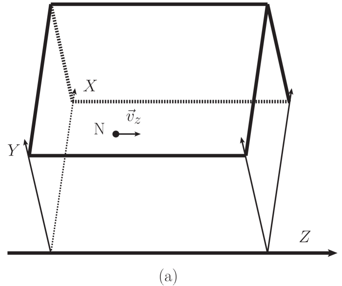
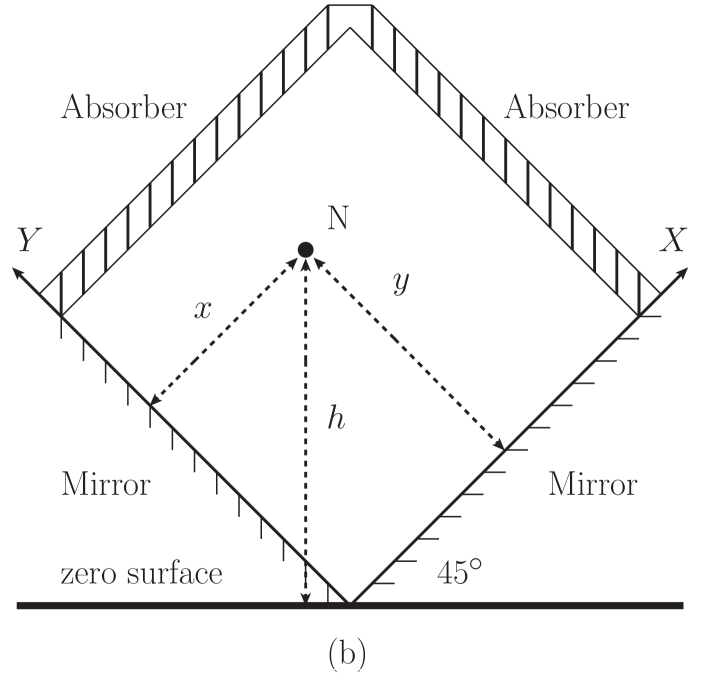
Figure 1: A rectangular cavity (RC) where the two lower surfaces are neutron mirrors and the two upper surfaces are neutron absorbers. In (a) a neutron N passes through the rectangular cavity with longitudinal velocity $\vec{v}_{z}$. (b) represents the transection of the rectangular cavity and $h$ is the height of the neutrons relative to the zero gravitational potential surface.

Now considering a specifically designed RC as shown in Fig.1, where the two lower surfaces of the cavity are neutron mirrors while the two upper surfaces are neutron absorbers. For each neutron in this cavity, it is subjected to a constant gravitational force $F=mg$. Together with the lower mirrors, the Earth’s gravitational field provides the confining potential well for the neutrons, which is

$$V(x,y)=\left\{\begin{array}[]{ll}mg(x+y)/\sqrt{2}&x\geq 0\;\text{and}\;y\geq 0\\ \\ +\infty&x<0\;\mathrm{or}\;y<0\end{array}\right.\;,$$ (9)

where we have chosen the zero potential surface in Fig. 1. In the transection of the cavity, the $X$-$Y$ plane of Fig. 1(b), the Schrödinger equation of motion for neutron takes the following form

$$-\frac{\hbar^{2}}{2m}\left(\frac{\partial^{2}}{\partial x^{2}}+\frac{\partial^{2}}{\partial y^{2}}\right)\Psi(x,y)+V(x,y)\Psi(x,y)=E\,\Psi(x,y)\;.$$ (10)

The energy eigenstates and eigenvalues of this equation can be similarly obtained as that of Eq.(4), and can be simply formulated as

$$\Psi_{n,m}(x,y)=\psi_{n}(x)\psi_{m}(y)\;,\;E_{n,m}=E_{n}+E_{m}\;.$$ (11)

Here, $\psi_{n}(x)=\mathcal{N}_{n}\,\mathrm{Ai}\left(x/l_{0}-E_{n}/\varepsilon_{0}\right)$, $\mathcal{N}_{n}$ is the normalization constant; $l_{0}$ and $\varepsilon_{0}$ are the characteristic length and energy defined as

$$l_{0} = \hbar^{2/3}/(\sqrt{2}m^{2}g)^{1/3}\simeq 6.59\cdot 10^{-6}\ \mathrm{m}\;,$$ (12)

$$\varepsilon_{0} = \sqrt[3]{mg^{2}\hbar^{2}/4}\simeq 4.78\cdot 10^{-13}\ \mathrm{eV}\;;$$ (13)

and $E_{n}=\alpha_{n}\varepsilon_{0}$ is the eigen energy of $\psi_{n}$ with $\alpha_{n}$ being defined after equation (5). The first four lowest eigenstates are $\Psi_{0,0}$, $\Psi_{0,1}$, $\Psi_{1,0}$, and $\Psi_{1,1}$, with $|\Psi_{n,m}(x,y)|^{2}$ being the value of the neutron probability density distributions in the $X$-$Y$ plane, see Fig. 2. Their corresponding energies can be listed as follows

$$E_{0,0} = E_{0}+E_{0}=\alpha_{0}\varepsilon_{0}+\alpha_{0}\varepsilon_{0}\simeq 2.22\times 10^{-12}\,\mathrm{eV}\;,$$ (14)

$$E_{0,1} = E_{0}+E_{1}=\alpha_{0}\varepsilon_{0}+\alpha_{1}\varepsilon_{0}\simeq 3.06\times 10^{-12}\,\mathrm{eV}\;,$$ (15)

$$E_{1,0} = E_{1}+E_{0}=\alpha_{1}\varepsilon_{0}+\alpha_{0}\varepsilon_{0}\simeq 3.06\times 10^{-12}\,\mathrm{eV}\;,$$ (16)

$$E_{1,1} = E_{1}+E_{1}=\alpha_{1}\varepsilon_{0}=\alpha_{1}\varepsilon_{0}\simeq 3.90\times 10^{-12}\,\mathrm{eV}\;,$$ (17)

where $E_{0,0}$ is the ground state energy and $E_{0,1}$ and $E_{1,0}$ are energies of the first degenerated excited states.

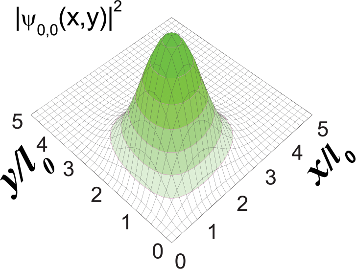
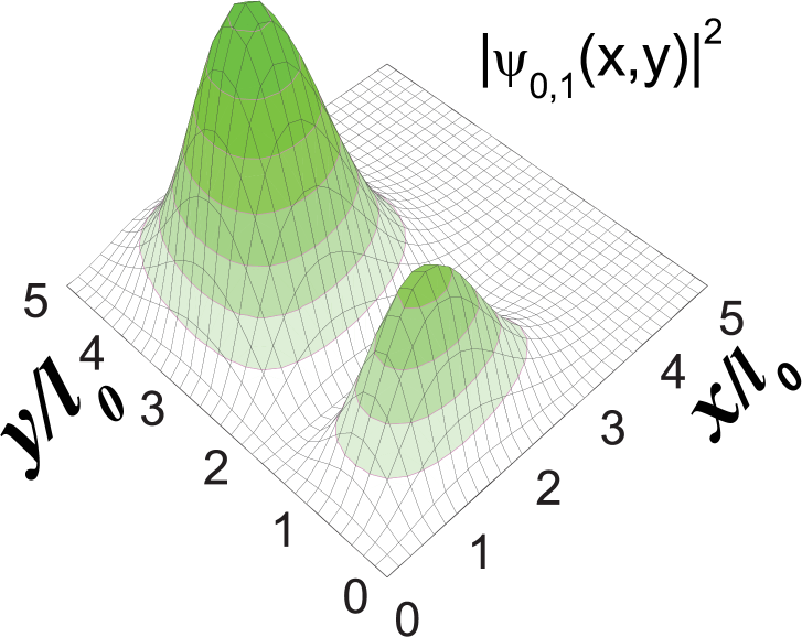
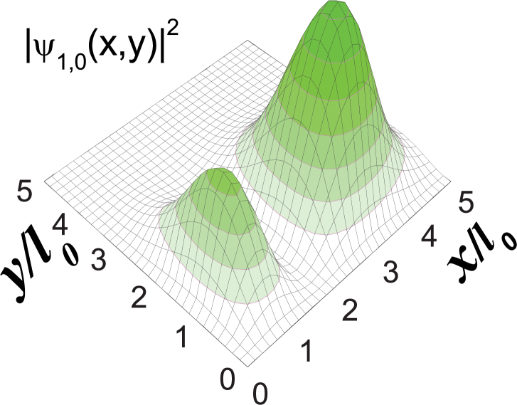
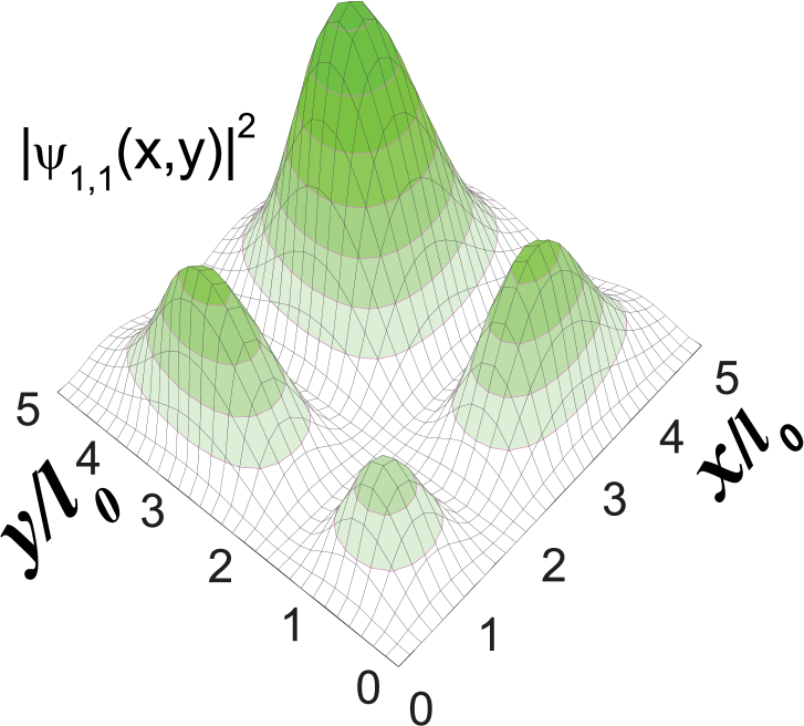
Figure 2: The probability density distributions of the first four lowest eigenstates in the transection of the rectangular cavity: $|\Psi_{0,0}|^{2}$, $|\Psi_{0,1}|^{2}$, $|\Psi_{1,0}|^{2}$, $|\Psi_{1,1}|^{2}$. The $X$ and $Y$ axes are in unit of $l_{0}$.

From the probability density distributions $|\Psi_{n,m}(x,y)|^{2}$ plotted in Fig. 2, we see that the quantum states of higher energies become densely distributed in the area with larger values of $x$, $y$. If the two upper absorbers are set at a position of $x=y\simeq 3l_{0}$, the transection of RC would have the size holding only the ground state. In this configuration, while the excited states $\Psi_{0,1}$, $\Psi_{1,0}$, $\Psi_{1,1}$ and other even higher excited states are substantially absorbed when the neutron transmitting in the cavity, the ground state survives. The minimal time $\tau_{g}$ while the neutron has to stay in the cavity to resolve different quantum states is [26]

$$\tau_{g}=\hbar/(E_{0,1}-E_{0,0})\sim 7.84\cdot 10^{-4}\mathrm{s}\;.$$ (18)

After a significantly longer time duration $T\gg\tau_{g}$ in the cavity, a substantial absorbtion of the excited state will be expected in the present configuration of $x=y\simeq 3l_{0}$.

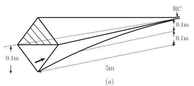
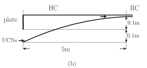
Figure 3: An HC coupled to the RC (a) and its longitudinal section (b). The whole HC can be made up of neutron mirrors. The arc in (b) is part of a circle with radius $62.6$m and is tangent to the horizontal RC at the joint. The UCN beam ejected into the HC from the lower half of the square (unshaded region in the (a)).

Now suppose a beam of monochromatic UCN with spectrum width $\Delta E$ is injected into a hopper like cavity (HC), which is coupled to RC as shown in Fig. 3. From the uncertainty relation $\Delta E\Delta t\sim\hbar$ and neutron energy $E=mv^{2}/2$, we cant get the coherent length of a single neutron in the monochromatic beam is $L_{c}=v\Delta t\sim\hbar/(m\Delta v)$. We propose the following condition on the monochromaticity of UCN

$$m(\Delta v)^{2}<(E_{0,1}-E_{0,0})\;.$$ (19)

Eq.(19) has two consequences: 1. There would not be enough kinetic energy for the neutron to knock another neutron to the excited states; 2. The relative displacement of two neutrons within the time interval $\tau_{g}$ is less than $L_{c}$. Now suppose one neutron approaches another neutron in the RC. When the distance between them is within the coherent length of $L_{c}$, the two neutrons become indistinguishable. As there is not enough energy to overcome the gap between $E_{0,1}$ and $E_{0,0}$ from any known types of interactions (see appendix C), the spatial wave functions of both neutrons will stay in the ground state and we have

$$\Psi^{(12)}(x_{1},y_{1};x_{2},y_{2})=\Psi_{0,0}(x_{1},y_{1})\Psi_{0,0}(x_{2},y_{2})\;,$$ (20)

where the indexes of the coordinates stand for the two neutrons. Due to the Pauli exclusive principles of the fermions, the spin wave function of the two neutrons then must be adjusted to the singlet state

$$\chi^{(12)}=\frac{1}{\sqrt{2}}(|+-\rangle-|-+\rangle)\;,$$ (21)

which is a spin entangled state.

In the following, we shall give an estimation for the practical experimental realization of our scheme. We take the UCNs with $v=5$ ms^-1 for numerical evaluation hereafter [27]. From the the condition of Eq.(19), the monochromatic UCN beam is characterized by

$$\Delta\lambda/\lambda=\Delta v/v<10^{-3}\;,$$ (22)

This monochromaticity could be achieved via a Drabkin energy filter [28] which is composed of a polarizer, spatial spin resonance (SSR) units, and a polarization analyzer. Using the superconducting solenoid-polarizer [29], the UCNs with different polarizations (parallel or antiparallel to magnetic field) have contrary behaviors: one polarization passes unhindered through the solenoid while the other polarization reflects backward. The degree of polarization of UCN can reach the level of $100\%$ [30]. The spatial spin resonance units only flip the spin of neutrons with specific wavelength (velocity) [28]. The polarization analyzer selects the spin flipped neutrons which now have the monochromatic wavelength (velocity). A precision of $\Delta\lambda/\lambda\simeq 10^{-2}$ has already been reached in [31] for neutrons with $\lambda=5\ \mathrm{\AA}$. As the resolution of the $\lambda$ is inversely proportional to the number of SSR units that neutrons pass through, an improvement to less than $10^{-3}$ is technically straight forward [32].

After the monochromatization, the UCN beam is then guided into the RC via HC, see Fig.3. The area of the entrance of HC is calculated to be $100\,\mathrm{cm}^{2}$. The collimation of the monochromatic beam should be $v_{x,y}/v_{z}<0.2$. That is $v_{x,y}<1\text{ms}^{-1}$, and the hight that the neutrons climb is less than $v_{x,y}^{2}/(2g)\sim 0.05\text{m}$. Thus all the UCNs that enter the HC can get into the RC. There, the number of UCNs which are within coherent length $L_{c}$ is $n_{c}=10\mathrm{cm}\times 10\mathrm{cm}\times L_{c}\times\rho_{\text{UCN}}$ where $\rho_{\text{UCN}}$ is the number density of UCN at the entrance of HC. In $t$ seconds there will be

$$N=n_{c}^{2}\times\frac{vt}{L_{c}}=vtL_{c}\rho^{2}_{\text{UCN}}\cdot(10^{4}\text{cm}^{4})$$ (23)

pairs of UCNs that are within the coherent length. Taking the value of $L_{c}\sim\hbar/(m\Delta v)\sim 7\times 10^{-4}\text{cm}$ into Eq.(23), we get $N\approx 3.5\times 10^{3}\text{cm}^{6}\text{s}^{-1}\cdot t\rho_{\text{UCN}}^{2}$. The polarized UCN density $\rho_{\mathrm{UCN}}=5\,\mathrm{cm}^{-3}$ has already been obtained [30], the monochromatization can further reduce this density by an order of $10^{-3}$ (estimated from Eq.(22)). Simple calculation shows that the production of one spin entangled UCN pair needs about 12 seconds, that is $3.5\times 10^{3}\cdot 12\cdot(5\times 10^{-3})^{2}=1.05$ pairs. If we adopt $\rho_{\mathrm{UCN}}=10\,\mathrm{cm}^{-3}$ for polarized UCNs then the same productivity consumes only three seconds.

Finally, the spin entangled UCN pairs appear at the exit of RC. To pick the entangled pairs from the stream of neutrons, we can use the time-of-flight measurements which guarantee that the detected two neutrons are originally within the coherent length in RC. As the entangled neutron pair leaves the RC, the two neutrons will move back to back in the $x-y$ plane due to the conservation of momentum. The out going entangled neutron pairs can be guided to sufficient long distance as the depolarization effect of UCN in collision with materials is quite low, $\sim 10^{-5}$ per collision [33]. The spin polarization analyzers can be applied to the well separated entangled neutrons, verifying their nonlocal correlations.

In conclusion, it is demonstrated that through a particular type of RC two neutrons immersed in the earth’s gravitational field will entangle with each other. The predicted production can be 1 entangled UCN pair in very few seconds. This enables us to test the quantum nonlocality involving the gravity, the only fundamental interaction of nature which has not yet been touched in practical entanglement generation so far. Due to the high detection efficiency of massive particle and the manageable large spatial separation between two neutrons (mean life of neutron at rest is $\tau\sim 885.7$s [34]), the proposed scheme also provides a simple and practical way for the implementation of nonlocality test of quantum entanglement and statistics in gravitational field, while a more conclusive test of local hidden variables theory would also be expected. Most importantly, our experimental scheme has been proved to be very feasible with the current technique, and a practical realization can be predicted in the very near future.

Acknowledgments

This work was supported in part by the National Natural Science Foundation of China(NSFC) under the grants 10935012, 10821063 and 11175249.

Appendix

A. Separation of the variables

Considering the potential of equation (9) in the region of $x\geq 0$, and $y\geq 0$, equation (10) can be expressed as

$$\left(-\frac{\hbar^{2}}{2m}\frac{\partial^{2}}{\partial x^{2}}+\frac{mgx}{\sqrt{2}}\right)\Psi(x,y)+\left(-\frac{\hbar^{2}}{2m}\frac{\partial^{2}}{\partial y^{2}}+\frac{mgy}{\sqrt{2}}\right)\Psi(x,y)=E\Psi(x,y)$$ (24)

Defining $\Psi(x,y)=\psi(x)\psi(y)$, the separation of variables, and $E=E_{x}+E_{y}$, the above equation can then be expressed as

$$\left\{\begin{array}[]{l}\left(\displaystyle-\frac{\hbar^{2}}{2m}\frac{\partial^{2}}{\partial x^{2}}+\frac{mgx}{\sqrt{2}}\right)\psi(x)=E_{x}\psi(x)\\ \\ \left(\displaystyle-\frac{\hbar^{2}}{2m}\frac{\partial^{2}}{\partial y^{2}}+\frac{mgy}{\sqrt{2}}\right)\psi(y)=E_{y}\psi(y)\end{array}\right.\;.$$ (28)

These two equations can be solved in the similar way as equation (5). The solutions are

$$\psi_{n}(x)=\mathcal{N}_{n}\,\mathrm{Ai}\left(x/l_{0}-E_{n}/\varepsilon_{0}\right)\;,\;\psi_{m}(y)=\mathcal{N}_{m}\,\mathrm{Ai}\left(y/l_{0}-E_{m}/\varepsilon_{0}\right)\;,$$

where $\mathrm{Ai}$ are Airy functions; $n,m\in\{0,1,2,\cdots\}$; $\mathcal{N}_{n}$ is the normalization constant; $l_{0}$, $\varepsilon_{0}$ are the characteristic length and energy defined as $l_{0}=\hbar^{2/3}/(\sqrt{2}m^{2}g)^{1/3}$, $\varepsilon_{0}=\sqrt[3]{mg^{2}\hbar^{2}/4}$.

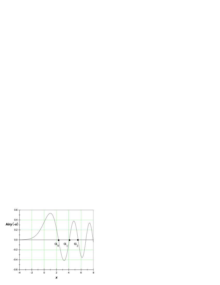
Figure 4: The zeros of Airy function: $\mathrm{Ai}(-\alpha_{n})=0$, $n\in\{0,1,2,\cdots\}$.

The eigenvalues of energy can be obtained by imposing the boundary condition $\psi_{n}(0)=\mathcal{N}_{n}\mathrm{Ai}(-E_{n}/\varepsilon_{0})=0$. We can get $E_{n}=\alpha_{n}\varepsilon_{0}$, where $\alpha_{n}$ is the $n$th zero of Airy function, see Figure 4.

B. Bouncing in the cavity

In the transection plane of the cavity, the ground state in the gravitational potential is $\Psi_{0,0}(x,y)=\psi_{0}(x)\psi_{0}(y)$. Inputting the numerical values $E_{0}$, $\mathcal{N}_{0}$ into the wave function we have

$$\Psi_{0,0}(x,y) \simeq \frac{25}{81}\mathrm{Ai}(x/6.59-2.34)\cdot\mathrm{Ai}(y/6.59-2.34)\;,$$ (29)

$$E_{0,0} = 2.22\cdot 10^{-12}\ \mathrm{eV}\;,$$ (30)

where $x$, $y$ are in unit of $\mu\mathrm{m}=10^{-6}\mathrm{m}$. In the ground state, $\langle x\rangle=\langle y\rangle\simeq 10.29\ \mu\mathrm{m}$, $\langle x^{2}\rangle=\langle y^{2}\rangle\simeq 126.89\ (\mu\mathrm{m})^{2}$, then $\Delta x=\Delta y=4.59\ \mu\mathrm{m}$. Due to the Heisenberg uncertainty relation $\Delta x\Delta p_{x}\geq\hbar/2$ and $p_{x}=mv_{x}$, we have $\Delta v_{x}\geq 6.86\cdot 10^{-3}\ \mathrm{ms}^{-1}$. The maximum velocity in $x$ axis is $v_{x\mathrm{max}}=\sqrt{2E_{0}/m}\simeq 1.46\cdot 10^{-2}\ \mathrm{ms}^{-1}$. The average velocity $\overline{v}_{x}$ in $x$ axis satisfies

$$\overline{v}_{x}=\frac{v_{x\mathrm{max}}}{2}\lesssim\Delta v_{x}\;.$$ (31)

The number of bouncing times of the neutron in the cavity is $n=\displaystyle\frac{T\cdot\overline{v}_{x}}{2l_{x}}$, where $l_{x}$ is the side length of the transection plane. The uncertainty of the bouncing times $n$ arises in regard of the variance $\Delta v_{x}$, and can be expressed as $\Delta n=\displaystyle\frac{T\Delta v_{x}}{2l_{x}}\gtrsim n$, which tells $\Delta n\geq 1$. Consequently, it is not distinguishable whether the neutron bounces in the cavity with odd or even number of times.

C. Magnetic dipole-dipole interaction

The energy of magnetic dipole-dipole interaction between two neutrons is

$$U=\frac{\mu_{0}}{4\pi}\frac{1}{|\vec{r}_{12}|^{3}}[\vec{\mu}_{1}\cdot\vec{\mu}_{2}-3(\vec{\mu}_{1}\cdot\vec{n})(\vec{\mu}_{2}\cdot\vec{n})]\;,$$ (32)

where $\mu_{0}$ is permeability of free space, $\vec{\mu}_{1,2}$ are the magnetic moment of the two neutrons, $|\vec{r}_{12}|$ is the distance between two neutrons and $\vec{n}=\vec{r}_{12}/|\vec{r}_{12}|$. The nearest distance between the two neutrons happens when they are in the same plane of transection of RC, then the distance can be expressed as

$$r_{12}^{2}=|\vec{r}_{12}|^{2}=(x_{1}-x_{2})^{2}+(y_{1}-y_{2})^{2}$$ (33)

the energy of magnetic dipole-dipole interaction between these two spin parallel neutrons (along $z$ direction) now becomes

$$U=\frac{\mu_{0}}{4\pi}\frac{\vec{\mu}_{1}\cdot\vec{\mu}_{2}}{|\vec{r}_{12}|^{3}}\;.$$ (34)

The expectation value $\langle r_{12}^{2}\rangle$ can be evaluated with the spatial wave function $\Psi_{12}(x_{1},y_{1};x_{2},y_{2})$ which is $\overline{r_{12}}=\sqrt{\langle r_{12}^{2}\rangle}\sim 9.2\mu\mathrm{m}$. At this distance the energy of spin-spin coupling of the two neutrons is roughly $U\sim 10^{-23}\mathrm{eV}$. This is negligibly small compare to the energy gap $E_{0,1}-E_{0,0}\sim 10^{-12}\mathrm{eV}$.

References

- [1] J.S. Bell, Physics 1, 195 (1964).
- [2] A. Aspect, P. Grangier, and G. Roger, Phys. Rev. Lett. 47, 460 (1981).
- [3] G. Weihs, et al, Phys. Rev. Lett. 81, 5039 (1998).
- [4] M. A. Rowe, et al, Nature 409, 791 (2001).
- [5] M. Ansmann, et al, Nature 461, 504 (2009).
- [6] H. Sakai, et al, Phys. Rev. Lett. 97, 150405 (2006).
- [7] P. Privitera, Phys. Lett. B 275, 172 (1992).
- [8] R. A. Bertlmann, Lecture Notes in Physics 689, 1 (2006).
- [9] Junli Li and Cong-Feng Qiao, Science China: Physics, Mechanics & Astronomy 53, 870 (2010).
- [10] Junli Li and Cong-Feng Qiao, Phys. Rev. D 74, 076003 (2006).
- [11] Junli Li and Cong-FengQiao, Phys. Lett. A 373, 4311 (2009).
- [12] Y. Makhlin, G. Schön, and A. Shnirman, Rev. Mod. Phys. 73, 357 (2001).
- [13] H. Häffner, C.F. Roos, and R. Blatt, Phys. Rep. 469, 155 (2008).
- [14] Jian-Wei Pan, et al, Rev. Mod. Phys. 84, 777 (2012).
- [15] R. Colella, A. W. Overhauser, and S. A. Werner, Phys. Rev. Lett. 34, 1472 (1975).
- [16] Magdalena Zych, et al , Nat. Commun 2, 505 (2011).
- [17] V.V. Nesvizhevsky,et al, Nature 415, 297 (2002).
- [18] R. T. Jones and E.G. Adelberger, Phys. Rev. Lett. 72, 2675 (1994).
- [19] C. R. Howell, et al, Phys. Lett. B 444, 252 (1998).
- [20] M. Avellino, S. Bose, and A. J. Fisher, arXiv:0807.1637
- [21] Y. Hasegawa, et al, Nature 425, 45 (2003).
- [22] K. Durstberger-Rennhofer and Y. Hasegawa, Physica B 406, 2373 (2011).
- [23] Yuji Hasegawa, et al, New J. Phys. 14, 023039 (2012).
- [24] S. Sponar, et al, New J. Phys. 14, 053032 (2012).
- [25] A. Y. Voronin, et al, Phys. Rev. D 73, 044029 (2006).
- [26] V. V. Nesvizhevsky, et al, Nucl. Instr. Meth. Phys. Res. A 440, 754 (2000).
- [27] H. Abele and H. Leeb, New. J. Phys. 14, 055010 (2012).
- [28] M. M. Agamalyan, G. M. Drabkin, and V. I. Sbitnev, Phys. Rep. 168, 265 (1988).
- [29] A. P. Serebrov, et al, Nucl. Instr. Meth. Phys. Res. A 545, 490 (2005).
- [30] A. P. Serebrov, et al, Nucl. Instr. Meth. Phys. Res. A 611, 263 (2009).
- [31] D. Yamazaki, et al, Nucl. Instr. Meth. Phys. Res. A 529, 204 (2004).
- [32] G. Badurek, Ch. Gösselsberger, and E. Jericha, Physica B 406, 2458 (2011).
- [33] A. P. Serebrov, et al, Phys. Lett. A 313, 373 (2003).
- [34] K. Nakamura, et al, Particle Data Group, J. Phys. G 37, 075021 (2010).