The Earliest Phases of Star formation observed with Herschel
(EPoS): The dust temperature and density distributions of B68

Abstract

Context. Isolated starless cores within molecular clouds can be used as a testbed to investigate the conditions prior to the onset of fragmentation and gravitational proto-stellar collapse.

Aims. We aim to determine the distribution of the dust temperature and the density of the starless core B68.

Methods. In the framework of the Herschel Guaranteed-Time Key Programme “The Earliest Phases of Star formation” (EPoS), we have imaged B68 between 100 and $500\leavevmode\nobreak\ \mu$m. Ancillary data at (sub)millimetre wavelengths, spectral line maps of the $\@element[12]{\mathrm{CO}}$ (2–1), and $\@element[13]{\mathrm{CO}}$ (2–1) transitions as well as an NIR extinction map were added to the analysis. We employed a ray-tracing algorithm to derive the 2D mid-plane dust temperature and volume density distribution without suffering from the line-of-sight averaging effects of simple SED fitting procedures. Additional 3D radiative transfer calculations were employed to investigate the connection between the external irradiation and the peculiar crescent-shaped morphology found in the FIR maps.

Results. For the first time, we spatially resolve the dust temperature and density distribution of B68, convolved to a beam size of 36$\aas@@fstack{\prime\prime}$4. We find a temperature gradient dropping from $(16.7{+1.3\above 0.0pt-1.0})$ K at the edge to $(8.2{+2.1\above 0.0pt-0.7})$ K in the centre, which is about $4$ K lower than the result of the simple SED fitting approach. The column density peaks at $N_{\mathrm{H}}=(4.3{+1.4\above 0.0pt-2.8})\leavevmode\nobreak\ \times 10^{22}$ cm^-2, and the central volume density was determined to $n_{\mathrm{H}}=(3.4{+0.9\above 0.0pt-2.5})\leavevmode\nobreak\ \times 10^{5}$ cm^-3. B68 has a mass of $3.1\leavevmode\nobreak\ M_{\sun}$ of material with $A_{K}>0.2$ mag for an assumed distance of 150 pc. We detect a compact source in the southeastern trunk, which is also seen in extinction and CO. At 100 and $160\leavevmode\nobreak\ \mu$m, we observe a crescent of enhanced emission to the south.

Conclusions. The dust temperature profile of B68 agrees well with previous estimates. We find the radial density distribution from the edge of the inner plateau outward to be $n_{\mathrm{H}}\propto r^{-3.5}$. Such a steep profile can arise from either or both of the following: external irradiation with a significant UV contribution or the fragmentation of filamentary structures. Our 3D radiative transfer model of an externally irradiated core by an anisotropic ISRF reproduces the crescent morphology seen at 100 and 160 $\mu$m. Our CO observations show that B68 is part of a chain of globules in both space and velocity, which may indicate that it was once part of a filament that dispersed. We also resolve a new compact source in the southeastern trunk and find that it is slightly shifted in centroid velocity from B68, lending qualitative support to core collision scenarios.

1 Introduction

There is a general consensus about the formation of low and intermediate-mass stars that they form via gravitational collapse of cold pre-stellar cores. A reasonably robust evolutionary sequence has been established over the past years from gravitationally bound pre-stellar cores (Ward-Thompson 2002) over collapsing Class 0 and Class I protostars to Class II and Class III pre-main sequence stars (André et al. 1993; Shu et al. 1987). The scenario of inside-out collapse of a singular isothermal sphere (e.g. Shu 1977; Young & Evans 2005) seems to be consistent with many observations of cores that already host a first hydrostatically stable protostellar object (e.g. Motte & André 2001). There are also disagreeing results in the case of starless cores, where inward motions exist before the formation of a central luminosity source (di Francesco et al. 2007), and infall can be observed throughout the cloud, not only in the centre (e.g. Tafalla et al. 1998).

Table 1: Details of the Herschel observations of B68.

OD	OBSID	Instrument	Wavelength	Map size	Repetitions	Duration	Scan speed	Orientation
			($\mu$m)			(s)	(″ s-1)	(°)
287	1342191191	SPIRE	250, 350, 500	$9\arcmin\times 9\arcmin$	1	555	30	$\pm$ 42
320	1342193055	PACS	100, 160	$7\arcmin\times 7\arcmin$	30	4689	20	45
	1342193056				30	4568	20	135

Evans et al. (2001) and André et al. (2004) consider positive temperature gradients, which are caused by external heating and internal shielding, for their density profile models of pre-stellar cores. Although their results differed quantitatively, both come to the conclusion that the slopes of the density profiles in the centre of pre-stellar cores are significantly smaller than previously assumed. However, these temperature profiles were derived from radiative transfer models with certain assumptions about the local interstellar radiation field, but lack an observational confirmation.

To improve this situation and measure the dust temperature and density distribution in a realistic way, we used the imaging capabilities of the Photodetector Array Camera and Spectrograph (PACS) (Poglitsch et al. 2010) and the Spectral and Photometric Imaging Receiver (SPIRE) (Griffin et al. 2010) instruments on board the Herschel Space Observatory (Pilbratt et al. 2010) to observe the Bok globule Barnard~68 (B68, LDN 57, CB 82) (Barnard et al. 1927) as part of the Herschel Guaranteed Time Key Programme “The Earliest Phases of Star formation” (EPoS; P.I. O. Krause; e.g. Beuther et al. 2010, 2012; Henning et al. 2010; Linz et al. 2010; Stutz et al. 2010; Ragan et al. 2012) of the PACS consortium. With these observations, we close the important gap that covers the peak of the spectral energy distribution (SED) that determines the temperature of the dust. These observations are complemented by data that cover the SED at longer wavelengths reaching into the millimetre range.

Bok globules (Bok & Reilly 1947) like B68 are nearby, isolated, and largely spherical molecular clouds that in general show a relatively simple structure with one or two cores (e.g.  Larson 1972; Keene et al. 1983; Chen et al. 2007; Stutz et al. 2010). A number of globules appear to be gravitationally stable and show no star formation activity at all. Whether or not this is only a transitional stage depends on the conditions inside and around the individual object (e.g.  Launhardt et al. 2010) like its temperature and density structure, as well as external pressure and heating. Irrespective of the final fate of the cores and the globules that host them, such sources are ideal laboratories in which to study physical properties and processes that exist prior to the onset of star formation.

B68 is regarded as an example of a prototypical starless core. It is located at a distance of about 150 pc (de Geus et al. 1989; Hotzel et al. 2002b; Lombardi et al. 2006; Alves & Franco 2007) within the constellation of Ophiuchus and on the outskirts of the Pipe nebula. The mass of B68 was estimated to lie between 0.7 (Hotzel et al. 2002b) and $2.1\leavevmode\nobreak\ M_{\sun}$ (Alves et al. 2001b), which also relies on different assumptions for the distance. Previous temperature estimates were mainly based on molecular line observations that trace the gas and resulted in mean values of the entire cloud between 8 K and 16 K (Bourke et al. 1995; Hotzel et al. 2002a; Bianchi et al. 2003; Lada et al. 2003; Bergin et al. 2006). Dust continuum temperature estimates lie in the range of 10 K (Kirk et al. 2007). However, they usually lack the necessary spatial resolution and spectral coverage for a precise assessment of the dust temperature. Typically, the Rayleigh-Jeans tail is well constrained by submillimetre observations. However, the peak of the SED, which is crucial for determining the temperature, is measured either with little precision or too coarse a spatial resolution that is unable to sample the interior temperature structure.

The radial density profile of B68 is often represented by fitting a Bonnor-Ebert sphere (BES) (Ebert 1955; Bonnor 1956), where self gravity and external and internal pressure are in equilibrium. Based on deep near-infrared (NIR) extinction mapping, Alves et al. (2001b) show by using this scheme that B68 appears to be on the verge of collapse. However, this interpretation is based on several simplifying assumptions, e.g. spherical symmetry and isothermality that is supposed to be caused by an isotropic external radiation field. Pavlyuchenkov et al. (2007) have shown that even small deviations from the isothermal assumption can significantly affect the interpretation of the chemistry derived from spectral line observations, especially for chemically almost pristine prestellar cores like B68, and therefore also affect the balance of cooling and heating.

We demonstrate in this paper that none of these three conditions are met, and we conclude that even though the radial column density distribution can be fitted by a Bonnor-Ebert (BE) profile, any interpretation of the nature of B68 that is based on this assumption should be treated with caution.

2 Observations, archival data, and data reduction

2.1 Herschel

The details of the observational design of the scan map Astronomical Observing Templates (AOT) are given in Table 1. We observed B68 at 100, 160, 250, 350, and 500 $\mu$m using both the imagers of the Herschel Space Telescope, i.e. PACS and SPIRE in prime mode. We chose not to employ the SPIRE/PACS parallel mode in order to avoid the inherent disadvantageous side effects, such as beam distortion, reduced spatial sampling, and lower effective sensitivity, in particular introduced by an increased bit rounding in the digitisation of the data that especially affects areas with low surface brightness. In this way, we were able to benefit from the best resolution and sensitivity available. The latter advantage is especially crucial for the $100\leavevmode\nobreak\ \mu$m data that are needed to constrain the temperature well. The approximate area covered by these observations is indicated in Fig. 1.

The PACS data reduction comprised a processing to the Level 1 stage using the Herschel Interactive Processing Environment (HIPE, V6.0 user release, Ott 2010) of the Herschel Common Science System (HCSS, Riedinger 2009). For the refinement to the Level 2 stage, we decided to employ the Scanamorphos software (Roussel 2012), which provides the best compromise to date of a good recovery of the extended emission and, at the same time, a proper handling of compact sources. Still, the resulting background offset derived from all non-cooled telescopes (e.g. Spitzer and Herschel) remain arbitrary and are mainly influenced by the emission of the warm telescope and the data reduction techniques. For processing the SPIRE data, we used HIPE, V5.0 (software build 1892). For details of the reduction of the Herschel data, we refer to Launhardt et al. (in prep.).

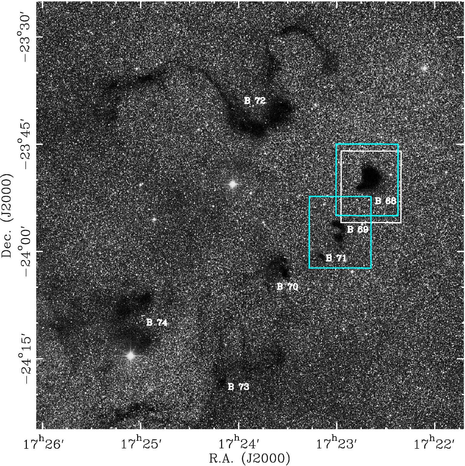
Figure 1: Digitized Sky Survey (red) image of the area around B68. The field-of-view (FoV) is $1\degr\times 1\degr$. The Barnard dark clouds 68 to 74 are indicated. The white frame represents the approximate FoV of the combined Herschel observations, while the blue frames denote the areas mapped in the $\@element[12]{\mathrm{CO}}$ and $\@element[13]{\mathrm{CO}}$ lines. North is up and east is to the left.

2.2 APEX

Observations with the Large APEX Bolometer Camera (LABOCA) (Siringo et al. 2009) attached to the Atacama Pathfinder Experiment (APEX) telescope (Güsten et al. 2006) at a wavelength of $870\leavevmode\nobreak\ \mu$m were carried out on 17 July 2007 with $2\times 2$ spiral patterns that were separated by $27\arcsec$. These observations were part of a programme aimed to cover a larger area, which will be presented in Risacher & Hily-Blant (in prep.). The original full width at half maximum ($FWHM$) of the main beam is 19$\aas@@fstack{\prime\prime}$2, but the maps were smoothed with a 2D Gaussian to reduce the background noise, resulting in an effective beam size of $27\arcsec$ matching the separation between individual observations. The absolute flux-calibration accuracy is assumed to be of the order of 15%. The root mean square (rms) noise in the map amounts to 5 mJy per beam.

The LABOCA data were reduced with the BoA software mainly following the procedures described in section 3.1 of Schuller et al. (2009). It comprised flagging bad and noisy channels, despiking, and removing correlated noise. In addition, low-frequency filtering was performed to reduce the effects of the slow instrumental drifts that are uncorrelated between bolometers. This filtering is performed in the Fourier domain, and applies to frequencies below 0.2 Hz, which, given the scanning speed of 3′ s^-1, translates to spatial scales of above 15′, i.e. larger than the LABOCA field of view.

The entire reduction was done in an iterative fashion. No source model was included for the first instance. Therefore, a first-order baseline removal was applied to the entire time stream. The signal above a threshold of $4\sigma$ obtained from result of the first reduction was then used as a source model in the second iteration to blank the regions. This iterative process was done five times in order to recover most of the extended emission.

The final map was created using a natural weighting algorithm in which each data point has a weight of $1/rms^{2}$, where $rms$ is the standard deviation assigned to each pixel.

2.3 Spitzer

B68 was observed with the Infrared Array Camera (IRAC, Fazio et al. 2004) on board the Spitzer Space Telescope (Werner et al. 2004) on 4 September 2004 in the framework of Prog 94 (PI: Lawrence). We used the archived data processed by the Spitzer Science Center (SSC) IRAC pipeline S18.7.0. Mosaics were created from the basic calibrated data (BCD) frames using a custom IDL program that is described in Gutermuth et al. (2008).

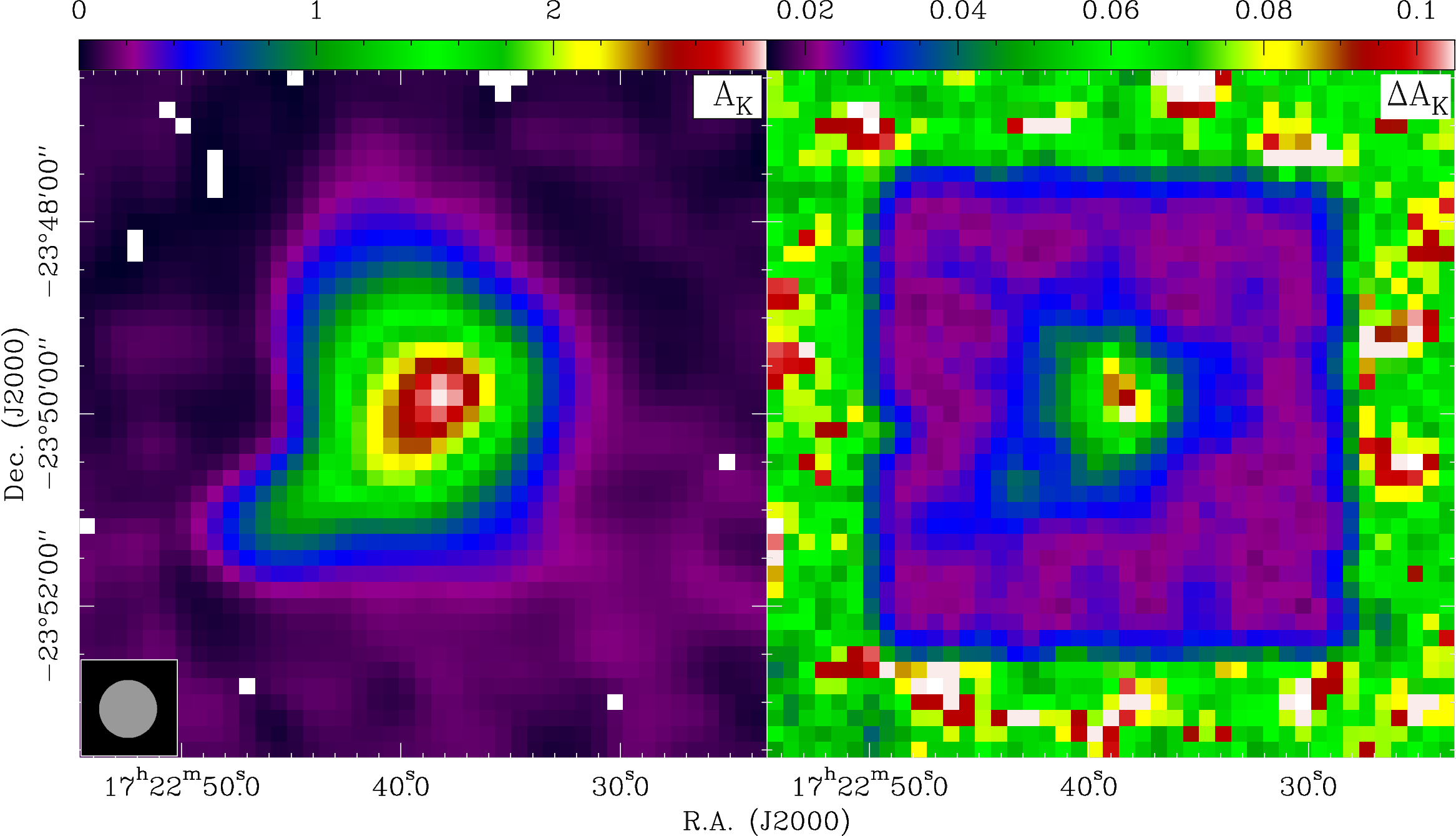
Figure 2: Distribution of $K$-band extinction $A_{K}$ recalculated from the data presented in Alves et al. (2001b) and complementary 2MASS data according to Sect. 2.5. Left: extinction map; right: corresponding error map. The original spatial resolution was convolved to match the SPIRE $500\leavevmode\nobreak\ \mu$m data. The spatial scale is the same as in Fig. 3.

In addition, we included 24 $\mu$m observations obtained with the Multiband Imaging Photometer for Spitzer (MIPS, Rieke et al. 2004). The observations were carried out in scan map mode during September 2004 and are part of programme 53 (PI: Rieke). Data reduction was done with the Data Analysis Tool (DAT; Gordon et al. 2005). The data were processed according to Stutz et al. (2007). These images are presented here for the first time.

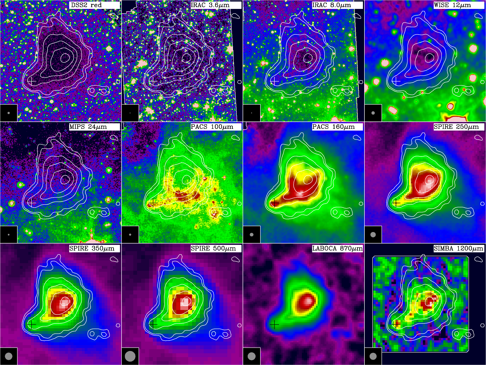
Figure 3: Image gallery of B68 Herschel and archival data covering a wide range of wavelengths. The instruments and wavelengths at which the images were obtained are indicated in the white annotation boxes. Each image has an arbitrary flux density scale, whose settings are given in Table 2. They were chosen to facilitate a comparison of the morphology. The maps are centred on RA $=17^{\mathrm{h}}22^{\mathrm{m}}39^{\mathrm{s}}$, Dec $=23\degr 50\arcmin 00\arcsec$ and have a field of view of $7\arcmin\times 7\arcmin$. All coordinates in this manuscript are based on the J2000.0 reference frame. The corresponding beam sizes are indicated in the inserts. Contours of the LABOCA data obtained at $\lambda=870\leavevmode\nobreak\ \mu$m show flux densities of 30, 50, 150, 250, 350, and 450 mJy/beam and are superimposed for comparison. The black and white crosses indicate the position of the point source at the tip of the trunk.

B68 was also observed with the Infrared Spectrograph (IRS, Houck et al. 2004) on board the Spitzer Space Telescope. With this instrument, low-resolution ($R\approx 60-120$) spectra were obtained on 23 March, 20 and 21 April 2005 in the framework of programmes 3290 (PI: Langer) and 3320 (PI: Pendleton). The spectra used in this paper are based on the droopres intermediate data product processed through the SSC pipeline S18.8.0. Partially based on the SMART software package (Higdon et al. 2004, for details on this tool and extraction methods), our data are further processed using spectral extraction tools developed for the FEPS Spitzer science legacy programme (for further details on our data reduction, see also Bouwman et al. 2008; Swain et al. 2008; Juhász et al. 2010). The spectra are extracted using a five-pixel fixed-width aperture in the spatial dimension for the observations in the first spectral order between 7.5 and 14.2 $\mu$m. Absolute flux calibration was achieved in a self-consistent manner using an ensemble of observations on the calibration stars HR~2194, HR~6606 and HR~7891 observed within the standard calibration programme for the IRS. The data were used for a different purpose than extracting the background emission spectra in Chiar et al. (2007).

2.4 Heinrich Hertz Telescope

Molecular line maps of the $\@element[12]{\mathrm{CO}}$ and $\@element[13]{\mathrm{CO}}$ species at the $J=2-1$ line transition (220.399 and 230.538 GHz) were obtained with the Heinrich Hertz Telescope (HHT) on Mt. Graham, AZ, USA. The field-of-view (FoV) of these observations is indicated in Fig. 1. The spectral resolution was $\approx 0.3$ km s^-1 and the angular resolution of the telescope was $32\arcsec$ ($FWHM$). For more details on the observations and data reduction, we refer to Stutz et al. (2009).

Table 2: Intensity cuts of the 12 images in Fig. 3.

	Low cut	High cut
Image label	(MJy sr-1)	(MJy sr-1)
DSS2 red	4900∗	10000∗
IRAC 3.6 $\mu$m	0.4	2.1
IRAC 8.0 $\mu$m	15.3	17.9
WISE 12 $\mu$m	13.6	14.2
MIPS 24 $\mu$m	0.0	0.4
PACS 100 $\mu$m	20.3	30.5
PACS 160 $\mu$m	7.4	42.0
SPIRE 250 $\mu$m	4.1	69.7
SPIRE 350 $\mu$m	2.0	50.4
SPIRE 500 $\mu$m	0.5	25.1
LABOCA 870 $\mu$m	0.0	6.7
SIMBA 1200 $\mu$m	0.0	4.1
∗ counts per pixel

2.5 Near-infrared dust extinction mapping

We used NIR data from the literature to derive the dust extinction through the B68 globule. Photometric observations of the sources towards the globule were performed in $JHK_{\mathrm{S}}$ bands by Alves et al. (2001b) and Román-Zúñiga et al. (2010) using the Son of ISAAC (SOFI) instrument (Finger et al. 1998; Moorwood et al. 1998) that is attached to the New Technology Telescope (NTT) at La Silla, Chile. The observed field of approximately $4\arcmin\times 4\arcmin$ only covers the innermost part of the globule. To estimate the extinction outside this area, we included photometric data covering a wider field from the Two Micron All Sky Survey (2MASS) archive (Skrutskie et al. 2006). For sources with detections in both 2MASS and SOFI data, the SOFI photometry was used (SOFI data were calibrated using 2MASS data, see Román-Zúñiga et al. 2010).

We used the $JHK_{\mathrm{S}}$ band photometric data in conjunction with the NICEST colour-excess mapping technique (Lombardi 2009) to derive the dust extinction. In general, the observed colours of stars shining through the dust cloud are related to the dust extinction via the equation

$$E_{i-j}=\left(m_{i}-m_{j}\right)-\left\langle m_{i}-m_{j}\right\rangle_{0}=A_{j}\left(\frac{\tau_{i}}{\tau_{j}}-1\right),$$ (1)

where $E_{i-j}$ is the colour-excess, $A_{j}$ extinction, and $\langle m_{i}-m_{j}\rangle_{0}$ the mean intrinsic colour of stars, i.e. the mean colour of stars in a control field that can be assumed to be free from extinction. This control field was chosen as a field of negligible extinction from the large-scale dust extinction map of the Pipe nebula (Kainulainen et al. 2009). When applying the NICEST colour-excess mapping technique, colour-excess measurements towards individual stars (observations in $JHK_{\mathrm{S}}$ bands yield two colour-excess measurements towards each star) are first combined using a maximum likelihood technique, yielding an estimate of extinction $A_{K}$ towards each detected source. Then, these measurements are used to produce a regularly sampled map of $A_{K}$ by computing the mean extinction in regular intervals (map pixels) using as weights the variance of each extinction measurement and a Gaussian-like spatial weighting function with $FWHM\approx 36\aas@@fstack{\prime\prime}4$ to match the resolution of the SPIRE $500\leavevmode\nobreak\ \mu$m observations. In deriving the extinction from Eq. 1, we adopted the coefficients for the reddening law $\tau_{i}$ from Cardelli et al. (1989):

$$\tau_{K}=0.600\cdot\tau_{H}=0.404\cdot\tau_{J}\quad.$$ (2)

The relation holds for the NIR extinction produced by the diffuse ISM and denser regions (e.g. Chapman et al. 2009; Chapman & Mundy 2009). The resulting $A_{K}$ extinction map is shown in Fig. 2.

The changes to the NIR extinction law introduced by varying $R_{V}=A_{V}/E(B-V)$ are insignificant. However, when extending the extinction law into the visual range, modifying $R_{V}$ between 3.1 and 5.0 changes $\tau_{J}/\tau_{V}$, $\tau_{H}/\tau_{V}$ and $\tau_{K}/\tau_{V}$ by approximately 16%. Since the values and the distribution of $R_{V}$ are a priori unknown, we use $A_{K}$ instead of $A_{V}$ in the subsequent ray-tracing modelling.

We select an empirical extinction law in the NIR instead of taking the opacities of the dust model of Ossenkopf & Henning (1994) as used for the subsequent modelling of the FIR to mm data. The reason is that by design this model does not account for scattering, which is an important contribution to the overall extinction in the NIR and difficult to predict, but which turns out to be negligible for FIR properties. Furthermore, Fritz et al. (2011) have shown that none of the currently available dust models can actually reproduce the observed NIR extinction properties well.

To visualise the different behaviours in the NIR range in Fig. 4, we compare the mass absorption coefficients of the dust model we use for the modelling and the ones obtained from the adopted empirical NIR extinction law via Eqs. 3 and 4:

$$\kappa_{\mathrm{d}}(\nu) = 6.02\times 10^{25}\mathrm{g}^{-1}\left(\frac{N_{\mathrm{H}}}{A_{\lambda}}\right)^{-1}$$ (3)

$$= 8800\leavevmode\nobreak\ \mathrm{cm}^{2}\mathrm{g}^{-1}\cdot R_{V}\cdot\left(\frac{A_{\lambda}}{A_{V}}\right)(R_{V})\quad.$$ (4)

They were derived by assuming a gas-to-dust ratio of 150 (Sodroski et al. 1997) and a conversion of the total gas to hydrogen mass of 1.36 (see Sect. A of the online appendix). In the NIR, $N_{\mathrm{H}}/A_{\lambda}$ can be determined using the estimates of Vuong et al. (2003) and Martin et al. (2012) along with the extinction law of Cardelli et al. (1989). For a discussion on the implicit assumptions and inherent uncertainties, we refer to Sect. 5.1.2.

Equation 4 provides a description that depends on $R_{V}$. Here, we adopted the relation $N_{\mathrm{H}}/A_{V}$ for the diffuse ISM ($R_{V}=3.1$) according to Güver & Özel (2009) and $A_{\lambda}/A_{V}$ as a function of $R_{V}$, following the extinction law of Cardelli et al. (1989, Eq. 1, Tab. 3). The numerical value for the ratio as established by Bohlin et al. (1978) is 10400 instead of 8800. As a result, $\kappa_{\mathrm{d}}(\nu)$ increases by a factor of 1.6 in the NIR when raising $R_{V}$ from 3.1 to 5.0. At the same time, the corresponding $N_{\mathrm{H}}$ value is reduced by $1-3.1/5.0=0.38$. This means that in dense cores, where $R_{V}$ is assumed to exceed the value of 3.1, the column density in the densest regions (i.e. the core centre) may be overestimated by this ratio when derived from $A_{V}$.

Figure 4: Dust opacities taken from Ossenkopf & Henning (1994) (coagulated, with thin ice mantles, $n_{\mathrm{H}}=10^{5}\mathrm{cm}^{-3}$) and from Cardelli et al. (1989), derived by using a gas-to-dust ratio of 150 (Sodroski et al. 1997). Different ratios of $N_{\mathrm{H}}/A_{\lambda}$ have been used (Vuong et al. 2003; Güver & Özel 2009; Martin et al. 2012) when applying Eqs 3 and 4. The insert shows an enlargement of the range covered by the $JHK$ bands.

For further details of the NICEST colour-excess mapping technique and for a discussion of its properties, we refer to Lombardi (2005, 2009).

2.6 Ancillary data

We included $450$ and $850\leavevmode\nobreak\ \mu$m data obtained with the Submillimetre Common-User Bolometer Array (SCUBA) at the James Clerk Maxwell Telescope (JCMT) at Mauna Kea, Hawaii, USA, in our analysis. These data were retrieved from the SCUBA Legacy Catalogues. The maps are not shown here, but have already been presented in di Francesco et al. (2008).

Observations at a wavelength of 1.2 mm were obtained with the SEST Imaging Bolometer Array (SIMBA) mounted at the Swedish-ESO Submillimetre Telescope (SEST) at La Silla, Chile. Standard reduction methods were applied as illustrated in Chini et al. (2003). For a detailed description of the data reduction, we refer to Bianchi et al. (2003). The map was also presented by Nyman et al. (2001).

Mid-infrared data obtained at $\lambda=12\leavevmode\nobreak\ \mu$m were taken from the data archive of the Wide-field Infrared Survey Explorer (WISE, Wright et al. 2010).

3 Modelling

3.1 Optical-depth-averaged dust temperature and column density maps from SED fitting

In a first step, we use the calibrated dust emission maps at the various wavelengths to extract for each image pixel an SED with up to eight data points between $100\leavevmode\nobreak\ \mu$m and 1.2 mm. For this purpose, they were prepared in the following way:

1. registered to a common coordinate system

2. regridded to the same pixel scale

3. converted to the same physical surface brightness

4. background levels subtracted

5. convolved to the SPIRE 500 $\mu$m beam

All these steps are described in detail in Launhardt et al. (in prep.). Nevertheless, we explain a few crucial procedures in more detail here. For all maps, the flux density scale was converted to a common surface brightness using convolution kernels of Aniano et al. (2011). In addition, we have applied a extended emission calibration correction to the SPIRE maps as recommended by the SPIRE Observers Manual.

The residual background offset levels to be subtracted from the individual maps were determined by an iterative scheme that uses Gaussian fitting and $\sigma$ clipping to the noise spectrum inside a common map area that was identified as being “dark” relative to the dust emission and relatively free of $\@element[12]{\mathrm{CO}}$ (2–1) emission. During each iteration, the flux range was extended until the distribution deviated from the Gaussian profile. This was only feasible because of the selection criterion of an isolated prestellar core.

The remaining emission seen by a given map pixel is then given by

$$S_{\nu}(\nu)=\Omega\left(1-e^{-\tau(\nu)}\right)\left(B_{\nu}(\nu,T_{\mathrm{d}})-I_{\mathrm{bg}}(\nu)\right)$$ (5)

with

$$\tau(\nu)=N_{\mathrm{H}}m_{\mathrm{H}}\frac{M_{\mathrm{d}}}{M_{\mathrm{H}}}\kappa_{\mathrm{d}}(\nu)$$ (6)

where $S_{\nu}(\nu)$ is the observed flux density at frequency $\nu$, $\Omega$ the solid angle from which the flux arises, $\tau(\nu)$ the optical depth in the cloud, $B_{\nu}(\nu,T_{\mathrm{d}})$ the Planck function, $T_{\mathrm{d}}$ the dust temperature, $I_{\mathrm{bg}}(\nu)$ the background intensity, $N_{\mathrm{H}}=2\times N(\mathrm{H}_{2})+N(\mathrm{H})$ the total hydrogen atom column density, $m_{\mathrm{H}}$ the hydrogen mass, $M_{\mathrm{d}}/M_{\mathrm{H}}$ the dust-to-hydrogen mass ratio, and $\kappa_{\mathrm{d}}(\nu)$ the dust opacity. For the purpose of this paper, we assume $T_{\mathrm{d}}$ and $\kappa_{\mathrm{d}}(\nu)$ to be constant along the LoS and discuss the uncertainties and limitations of this approach in Launhardt et al. (in prep.).

The fluxes of the radiation background $I_{\mathrm{bg}}(\nu)$ and the instrumental contributions from the warm telescope mirrors were removed during the background subtraction described above. Its exact values are unknown, but $I_{\mathrm{bg}}(\nu)$ is dominated by contributions from the cosmic infrared and microwave backgrounds, as well as the diffuse galactic background. A detailed investigation shows that $I_{\mathrm{bg}}\ll B_{\nu}(10\leavevmode\nobreak\ \textrm{K})$, so that neglecting this contribution introduces a maximum uncertainty of 0.2 K to the final dust temperature estimate.

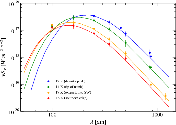
Figure 5: Spectral energy distributions at four selected positions across B68. The dots represent $10\arcsec\times 10\arcsec$ pixel values extracted from the maps that are used for the modified black body fitting. The solid curves are the SEDs fitted for a given dust temperature and column density.

For the dust opacity, $\kappa_{\mathrm{d}}(\nu)$, we use the tabulated values listed by Ossenkopf & Henning (1994) for mildly coagulated ($10^{5}$ yrs coagulation time at gas density $10^{5}$ cm^-3) composite dust grains with thin ice mantles. The resulting optical depth averaged dust temperature and column density maps are presented in Sect. 4.3. They provide an accurate estimate to the actual dust temperature and column density of the outer envelope, where the emission is optically thin at all wavelengths and LoS temperature gradients are negligible. Towards the core centre, where cooling and shielding can produce significant LoS temperature gradients and the observed SEDs are therefore broader than single-temperature SEDs, the central dust temperatures are overestimated and the column density is underestimated. Since this effect gradually increases from the edges to the centre of the cloud, the resulting radial column density profile mimics a slope that is shallower than the actual underlying radial distribution.

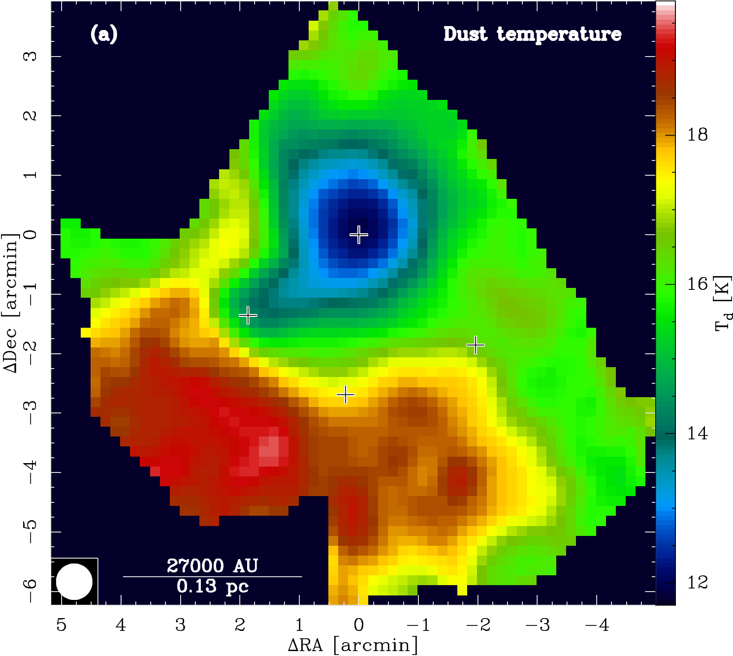
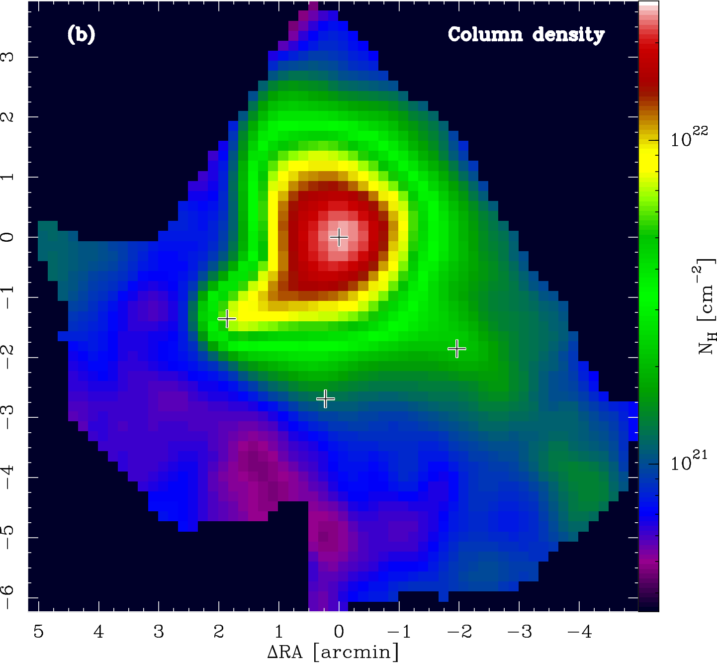
Figure 6: Dust temperature (a) and column density (b) maps of B68 derived by line-of-sight SED fitting as described in Sect. 3.1. The temperature minimum attains 11.9 K and is offset by $5\arcsec$ from the column density peak. The four positions from which we extracted the individual SEDs shown in Fig. 5 are indicated with $+$. The central column density is $N_{\mathrm{H}}=2.7\times 10^{22}$ cm^-2. The coordinates are given in arcminutes relative to the centre of the column density distribution, i.e. RA $=17^{\mathrm{h}}22^{\mathrm{m}}38\aas@@fstack{s}6$, Dec $=-23\degr 49\arcmin 51\arcsec$.

This procedure is illustrated in Fig 5, where the SEDs based on the map pixel fluxes at four positions in the B68 maps are plotted and fitted. This process includes an iterative colour correction for each of the derived temperatures. We chose four exemplary locations that cover the full temperature range, i.e. at the peak of the column density, at the tip of the southeastern extension (the trunk) within the faint extension to the southwest where the $870\leavevmode\nobreak\ \mu$m map has a faint local maximum, and towards the southern edge of B68 (see Fig. 6). The fits to the SEDs demonstrate that the flux levels are very consistent with a flux distribution of a modified Planck function. Only the $100\leavevmode\nobreak\ \mu$m data are generally too high for the coldest temperatures, which we attribute to contributions from higher temperature components along the LoS. We have assigned a reduced weight in the single-temperature SED fitting to them. The reason for them being at a similar level irrespective of the map position is related to the small flux density contrast in the $100\leavevmode\nobreak\ \mu$m map (Tab. 2). Also physical effects like stochastic heating of very small grains (VSGs) may play a role, but dealing with these issues is beyond the scope of this paper.

3.2 Dust temperature and density structure from ray-tracing models

In a second step, we attempt to reconstruct an estimate of the full temperature and density structure of the cloud by accounting for LoS temperature and density gradients in the SED modelling. We make the simplifying starting assumption of spherical geometry, i.e. we assume that the LoS profiles are equal to the mean profiles in the plane of the sky (PoS), but then allow for local deviations. For this purpose, we construct a cube with the $x$ and $y$ dimension and pixel size equal to the flux maps and 100 pixels in the $z$ direction. Each cell in this cube represents a volume element of the size $(10\,D_{\mathrm{p}c}\,\mathrm{AU})^{3}$, where 10 is the chosen angular pixel size in arcseconds and $D_{\mathrm{p}c}$ is the distance towards the source in pc, resulting in a resolution of $1.13\times 10^{49}$ cm³ per cell. Each cell is assigned a density and a temperature. We start with a spherical model centred on the column density peak derived by the LoS SED fitting (Sect. 3.1) and at the cube centre in $z$ direction. For the density profile, we assume a “Plummer-like” function (Plummer 1911)

$$n_{\mathrm{H}}(r)=n_{0}\left(\frac{r_{0}}{\left(r_{0}^{2}+r^{2}\right)^{1/2}}\right)^{\eta}=\frac{n_{0}}{\left(1+\left(\frac{r}{r_{0}}\right)^{2}\right)^{\eta/2}}\quad,$$ (7)

introduced by Whitworth & Ward-Thompson (2001) to characterise the radial density distribution of prestellar cores on the verge of gravitational collapse. It is analytically identical to the Moffat profile (Moffat 1969) and can also mimic a BES density profile very closely for a given choice of parameters. To account for the observed outer density “plateau”, we modify it by adding a constant term:

$$n_{\mathrm{H}}(r)=\left\{\begin{array}[]{ll}\frac{\Delta n}{\left(1+\left(\frac{r}{r_{\mathrm{0}}}\right)^{2}\right)^{\eta/2}}+n_{\mathrm{out}}&\mbox{ if $r\leq r_{\mathrm{out}}$}\\ 0&\mbox{ if $r>r_{\mathrm{out}}$}\quad.\end{array}\right.$$ (8)

The radius $r_{\mathrm{out}}$ sets the outer boundary of the modelling. Anything beyond this radius is set to zero. The peak density is then

$$n_{0}=n_{\mathrm{out}}+\Delta n\quad.$$ (9)

Adding a constant term to Eq. 7 slightly changes the behaviour of $r_{0}$ and $\eta$. Although this complicates comparing the results with previous findings, we apply Eq. 8 to analytically describe the radial distribution for the ray-tracing fitting, because it simplifies the modelling and fits better to the radial profiles than Eq. 7. This profile (i) accounts for an inner flat density core inside $r_{0}$ with a peak density $n_{0}$, (ii) approaches a modified power-law behaviour with an exponent $\eta$ at $r\gg r_{0}$, (iii) turns over into a flat-density halo outside

$$r_{1}=r_{\mathrm{0}}\,\sqrt{\left(\frac{\Delta n}{n_{\mathrm{out}}}\right)^{2/\eta}-1}\quad,$$ (10)

which probably belongs to the ambient medium around and along the LoS of B68, and (iv) is manually cut off at $r_{\mathrm{out}}$. The outer flat-density halo and the sharp outer boundary are artificial assumptions to simplify the modelling and account for the observed finite outer halo. This outer tenuous envelope of material is neither azimuthally symmetric nor fully spatially covered by our observations. Therefore, its real size remains unconstrained. Furthermore, its temperature and density remain very uncertain because of the low flux levels and uncertainties introduced by the background and its attempted subtraction. Therefore, the value of $r_{\mathrm{out}}$ should not be considered as an actual source property.

Table 3: Parameters and results of the ray-tracing modelling for the radial distributions using Eq. 8.

		$T$			$N_{\mathrm{H}}$			$n_{\mathrm{H}}$
		(K)			$(10^{20}\leavevmode\nobreak\ \mathrm{cm}^{-2})$			$(10^{2}\leavevmode\nobreak\ \mathrm{cm}^{-3})$			LoS				PoS
Solution		0	out		0	out		0	out		$\tau_{0}$	$r_{0,n}\leavevmode\nobreak\ (\arcsec)$	$\eta_{n}$		$\tau_{0}$	$r_{0,N}\leavevmode\nobreak\ (\arcsec)$	$\eta_{N}$	$r_{0,n}\leavevmode\nobreak\ (\arcsec)$	$\eta_{n}$
best		8.2	16.7		430	8		3400	4		1.5	35	4.0		2.1	76	4.6	56	4.9
steep		9.7	16.7		450	9		2600	5		3.0	40	3.5		3.3	99	6.7	77	6.6
flat		8.2	17.0		350	8		2200	1		0.5	40	3.7		1.8	85	4.9	48	3.7

For the temperature profile of an externally heated cloud, we adopt the following empirical prescription. It resembles the radiation transfer equations in coupling the local temperature to the effective optical depth towards the outer “rim”, where the ISRF impacts:

$$T(r)=T_{\mathrm{out}}-\Delta T\left(1-e^{-\tau(r)}\right)$$ (11)

with

$$\Delta T=T_{\mathrm{out}}-T_{0}\quad,$$ (12)

the frequency-averaged effective optical depth

$$\tau(r)=\tau_{0}\int_{r}^{r_{\mathrm{out}}}\frac{n_{\mathrm{H}}(x)}{n_{0}}\,dx\quad,$$ (13)

and $\tau_{0}$ being an empirical (i.e. free) scaling parameter that accounts for the a priori unknown mean dust opacity and the UV shape of the ISRF. The constant term $T_{0}$, which is also free in the modelling, accounts for the additional IR heating (external and internal). The functional shape of this simple model was compared to results of full radiative transfer simulations over a range of parameters relevant for this study (e.g. Zucconi et al. 2001) and found to agree reasonably well.

This description has a total of eight free parameters, of which $r_{\mathrm{out}}$ and $T_{\mathrm{out}}$ are derived from the azimuthally averaged profile of the column density map resulting from the SED fitting (Sect. 3.1) and are then kept fixed. The parameters $r_{0}$, $\eta$, and $n_{\mathrm{out}}$ are estimated from the same source, but then are iterated via the azimuthally averaged profile of the resulting volume density map. $\tau_{0}$ is initially set to 1 and is then also iterated via the azimuthally averaged profiles of the resulting volume density and mid-plane temperature maps. Finally, $n_{0}$ and $\Delta T$ are derived independently for each image pixel by ray-tracing through the model cloud and least squares fitting to the measured SEDs. An iterative colour correction algorithm was applied for each of the derived temperatures. At $r>r_{1}$, the cloud is assumed to be isothermal, and we fit for a single $T$ instead of a temperature profile with $\Delta T$. The best-fit solutions for all image pixels are checked to be unique in all cases, albeit with non-negligible uncertainty ranges, i.e. the fit never converges to local (secondary) minima.

This procedure yields cubes of density and temperature values, from which we extract the mid-plane (in the PoS) density and temperature maps, as well as the total column density map (by integrating the density cube along the LoS). The resulting mid-plane density and temperature maps are then azimuthally averaged and fitted for $n_{0}$, $r_{0}$, $\eta$, $n_{\mathrm{out}}$, and $\tau_{0}$. The resulting best-fit values are then used to update the LoS profiles of the model for the next ray-tracing iteration. Approximate convergence between the input LoS profile parameters and the PoS profiles derived from the mid-plane density and temperature maps of the independently fitted image pixels is usually reached after two to three iterations. To account for beam convolution effects in the PoS, we use a slightly smaller $r_{0}$ along the LoS than derived in the PoS. This procedure allows us to fit for local deviations from the spherical profile in the plane of the sky, while preserving the on average symmetric profile along the LoS.

Since this iteration between PoS and LoS profiles does not lead to a well-defined exact solution, we derive the uncertainties on the density and temperature values not simply from the formal statistical fitting errors, but proceed as follows. Once we have a parameter set for which PoS and LoS profiles converge, we decrease and increase $\tau_{0}$ by a factor of two and adjust the other parameters for the LoS profile such that we obtain the smoothest possible PoS profile; convergence between PoS and LoS is no longer reached with these $\tau_{0}$ values. A larger $\tau_{0}$ representing a better shielding leads to a steeper drop of $T$ with a wide inner plateau of nearly constant $T_{0}$ at a higher value than in the best-fit case. A smaller $\tau_{0}$ simulating a weaker shielding leads to a shallower drop of $T$ with a small inner region of very low $T_{0}$. To this range of profiles we add the statistical fitting uncertainties to define the total uncertainty, as illustrated in Fig. 7. We have listed the corresponding parameters used for the LoS and the PoS fitting in Table 3. The resulting temperature and density profiles calculated along the LoS provide a significantly better approximation to the true underlying source structure than the results of the single SED fitting; in the isothermal SED analysis, the individual pixel SEDs represent average LoS quantities projected to the PoS.

4 Results

4.1 From absorption to emission

As shown by Fig. 3, B68 causes extinction from the optical to the mid-IR (MIR) range. Various authors have used this property to derive extinction maps (e.g.  Alves et al. 2001b; Lombardi et al. 2006; Racca et al. 2009) and determine its density distribution. We have augmented the data of Alves et al. (2001b) with the 2MASS catalogue (Skrutskie et al. 2006) to extend the resulting size of the extinction map (Fig. 2) so that it matches the extents and resolution of the Herschel maps (see Sect. 2.5).

The absorption that is seen at the Spitzer IRAC 8 $\mu$m and the WISE 12 $\mu$m bands is most likely caused by the attenuation of background emission originating in polycyclic aromatic hydrocarbons (PAHs) by the dust in B68. Such spectral features are visible in Spitzer IRS background spectra (available as online material, Fig. 19) at prominent wavelengths (8.6, 11.3, 12.7 $\mu$m) without any spatial variation across B68. This indicates that the emission is dominated by contributions from the ambient diffuse interstellar medium (ISM) and is not related to B68 itself.

There is no evidence for coreshine (Steinacker et al. 2010) in the Spitzer IRAC 3.6 and 4.5 $\mu$m images. Since coreshine is interstellar radiation scattered by dust grains larger than the majority of grains in the ISM, it could indicate that grain growth is or has been inefficient in B68. Only about half of the cores investigated so far show the effect (Stutz et al. 2009; Pagani et al. 2010).

In the $24\leavevmode\nobreak\ \mu$m maps, B68 appears as neither a clear absorption nor an emission feature. The low dust temperatures cause the thermal emission to remain well below the MIPS $24\leavevmode\nobreak\ \mu$m detection limit. Since the extinction law is very similar at 8, 12, and 24 $\mu$m (Flaherty et al. 2007), the lack of the absorption feature may be attributed to the missing strong background emission that is present as PAH emission in the 8 and 12 $\mu$m images. The inherent contrast between emission and absorption at $24\leavevmode\nobreak\ \mu$m could be below the detection limit of the MIPS observations. It is not until $100\leavevmode\nobreak\ \mu$m that B68 appears faintly in emission above the diffuse signal from the surrounding ISM, mainly in the southern part of the globule (see next Sect.). As seen in Fig. 5, the maximum of the SEDs is between 100 and 250 $\mu$m.

4.2 Morphology

Based on observations at visual, near-infrared (NIR), and millimetre (mm) wavelengths, the morphology of B68 is usually described in terms of a nearly spherical globule with a small extension to the southeast (e.g.  Bok 1977; Nyman et al. 2001). This is also confirmed by extinction maps that are based on NIR imaging as shown in Fig. 2 (Alves et al. 2001b; Racca et al. 2009). However, the spatial distribution of the far-infrared (FIR) emission as measured by Herschel depends on the observed wavelength and does not show the symmetry that one would expect by extrapolating from previous observations.

At 100 $\mu$m (Fig. 3, second row, second column), B68 is dominated by a rather faint extended emission that almost blends in with the ambient background emission. The brightest region forms a crescent that covers the southern edge of the globule and resembles the distribution of C¹⁸O gas as shown by Bergin et al. (2002). The peak of the $100\leavevmode\nobreak\ \mu$m emission is not located at the position of the highest extinction. As shown by the superimposed LABOCA map, there is a gap of emission instead. A handful of background stars also detected at shorter wavelengths is present in this map. The southeastern extension is also visible.

The morphology is still present at 160 $\mu$m (Fig. 3, second row, third column), where the crescent-shaped extended emission is even more pronounced. As the observed wavelength increases, the crescent-shaped feature converges to the more familiar morphology observed in, e.g., near-IR extinction and long wavelength continuum data (c.f. Fig. 3, third row, third column). In Sect. 5.2, we demonstrate that this changing morphology can be explained by anisotropic irradiation effects. It is interesting that the MIR images, in particular at 8 and $12\leavevmode\nobreak\ \mu$m, show a brightness gradient from the north to the south. Drawing a connection to the anisotropic irradiation also in these wavebands appears tempting, because they contain prominent spectral bands of PAH emission from VSGs that might be induced by an incident UV field. However, the actual nature of the excess emission south of B68 is uncertain (PAH or continuum emission) and there is no evidence of a physical connection of that emission to B68 (see also the discussion on PAH emission in the previous section). Therefore, we leave a more detailed analysis of this phenomenon to later studies.

At the tip of the southeastern extension, there appears to be a compact object whose detection is confirmed by the Herschel 160 $\mu$m and 250 $\mu$m maps, indicated in Fig. 3, and by our $\@element[13]{\mathrm{CO}}$ (2–1) mean intensity map (Fig. 10). It is also present in the extinction map of Alves et al. (2001a). There is a point source $15\arcsec$ east of that position in the 100 $\mu$m map, but this one corresponds to a background source that is also visible in the Spitzer images. The newly discovered source disappears and blends in with the more extended emission at longer wavelengths, but reappears at 1.2 mm. We successfully performed PSF photometry of this feature in the two PACS bands, while we used the background star visible in the 100 $\mu$m map as an upper limit for the true flux at this position. A calibration observation of the asteroid Vesta obtained during the operational day (OD) 160 of the Herschel mission was selected to serve as a template for the instrumental point spread function (PSF). With a PSF fitting correlation coefficient of $>80\%$, we find a point source at RA $=17^{\mathrm{h}}22^{\mathrm{m}}46\aas@@fstack{s}3$, Dec $=-23\degr 51\arcmin 15\arcsec$ (see Fig. 3), where the visual extinction attains $A_{V}=11.3$ mag. The photometry yields colour-corrected flux densities of $(20.0\pm 0.5)$ mJy at 100 $\mu$m and $(178.5\pm 1.4)$ mJy at 160 $\mu$m. By fitting a Planck function, we derive a formal colour temperature of 15 K, i.e. the true colour temperature is even lower, since the 100 $\mu$m flux is taken as an upper limit. A mass estimate can be attempted by using the relation

$$M_{\mathrm{H}}=m_{\mathrm{H}}\sum_{\mathrm{\#pix}}N_{\mathrm{H}}A_{\mathrm{pix}}\quad.$$ (14)

We applied it to the extinction map of Alves et al. (2001b), which has a better resolution than the Herschel-based density maps. The pixel scale is $5\arcsec\times 5\arcsec$, resulting in a pixel area of $A_{\mathrm{pix}}=1.26\times 10^{32}$ cm² at an assumed distance of 150 pc. The conversion factor of $N_{\mathrm{H}}/A_{V}=2.2\times 10^{21}$ cm^-2 mag^-1 (Ryter 1996; Güver & Özel 2009; Watson 2011) was applied. Then we extracted the source from this map via a 2D Gaussian fit after an unsharp masking procedure by convolving the original extinction map to three resolutions, $30\arcsec$, $40\arcsec$ and $50\arcsec$. The resulting extracted mass is of the order of $M_{\mathrm{tot}}=1.36\leavevmode\nobreak\ M_{\mathrm{H}}=8\times 10^{-2}\leavevmode\nobreak\ M_{\sun}$.

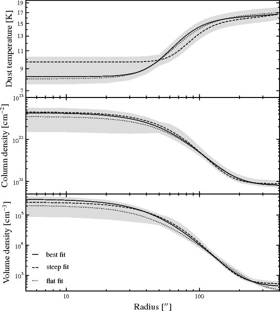
Figure 7: Visualisation of the ray-tracing fitting to the B68 data according to Table 3. We show the functional relations we used for fitting the LoS distributions of the dust temperature and the volume density that cover the range of valid solutions for each of the modelled quantities. The column density is the result of the integration of modelled volume densities along the LoS. The shaded areas represent the modelled range of values including the uncertainties of the fitting algorithm. Only the best fits (solid lines) are used to create the maps that show the dust temperature, the column density, and the volume density distributions.

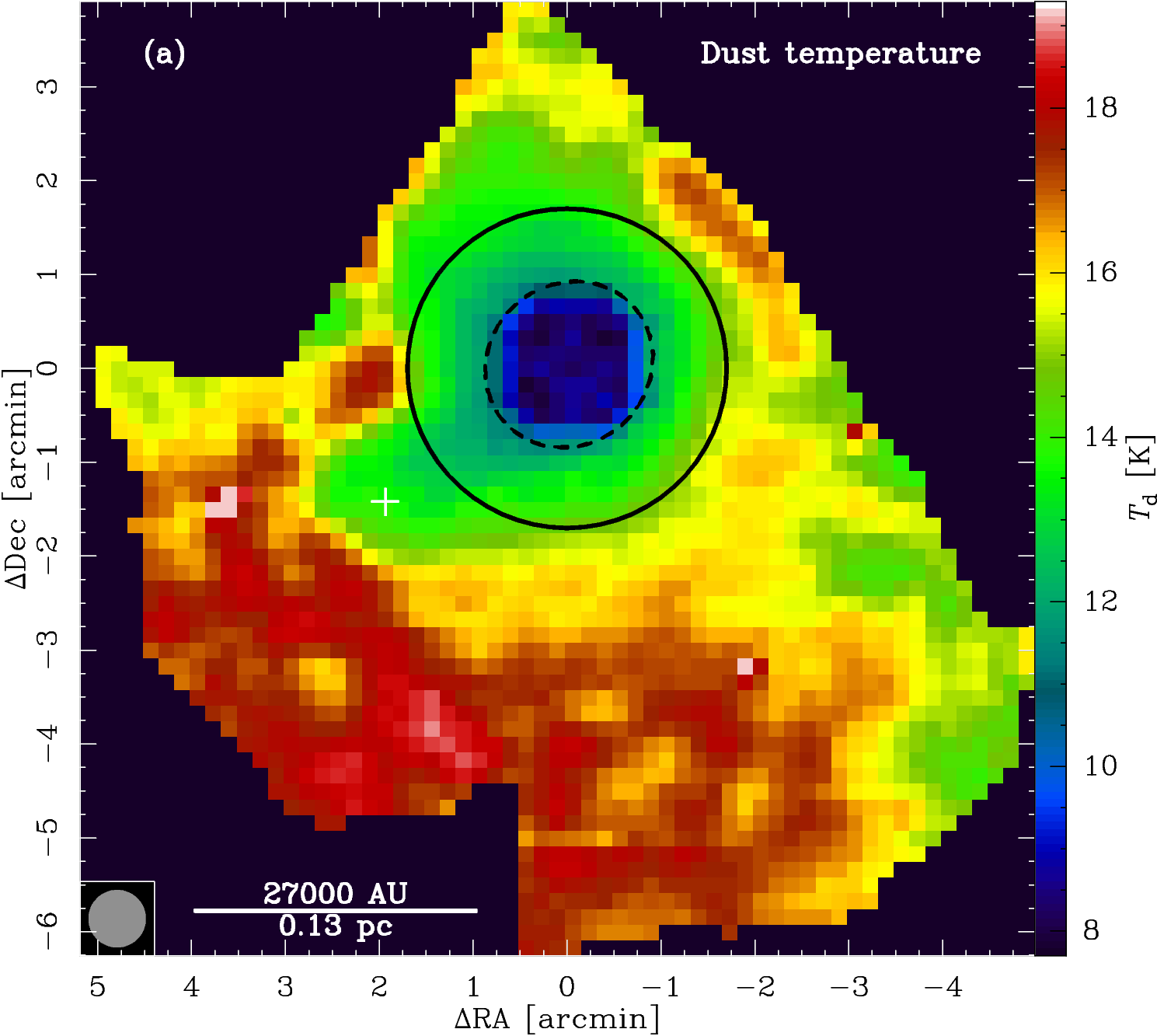
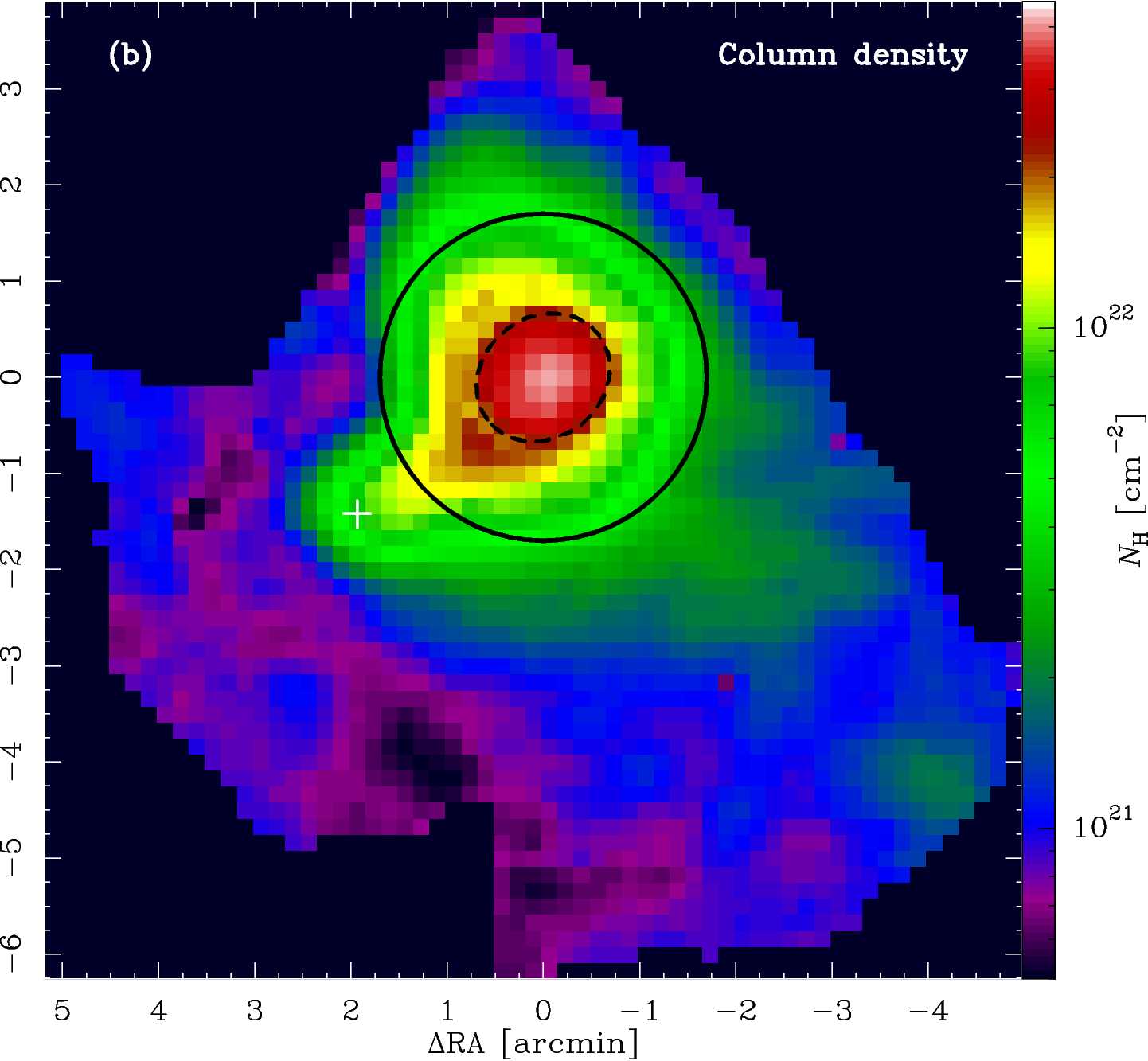
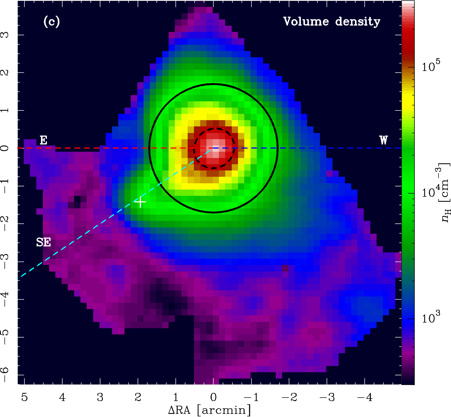
Figure 8: Dust temperature (a), column density (b), and volume density (c) maps of B68 derived by the ray-tracing algorithm as described in Sect. 3.2. The maps showing the dust temperature and the volume density are the ones calculated for the mid-plane across the plane of the sky. The global temperature minimum coincides with the density peak and attains a value of 8 K. The central column density is $N_{\rm H}=4.3\times 10^{22}$ cm^-2. The central particle density is $n_{\rm H}=3.4\times 10^{5}$ cm^-3. The black solid circles represent the size of the BES fitted by Alves et al. (2001b). The major and the minor axes of the black dashed ellipses denote the $FWHM$ of the 2D Gaussians fitted to temperature and density peaks (see text). We have plotted the three cuts through the maps as dashed lines, whose colours match the ones in the radial profile plots. The white crosses indicate the location of the point source we have identified and described in Sect. 4.2. The coordinates are given in arcminutes relative to the centre of the density distributions, i.e. RA $=17^{\mathrm{h}}22^{\mathrm{m}}38\aas@@fstack{s}5$, Dec $=-23\degr 49\arcmin 50\arcsec$.

4.3 Line-of-sight-averaged SED fitting: Temperature and column density distribution

To illustrate the differences between the two modelling approaches, we briefly summarise the results of the modified black body fitting in this section. The procedure is illustrated in Fig. 5, where the SEDs based on the map pixel fluxes at four positions in the B68 maps (see Fig. 6) are plotted and fitted. We chose four exemplary locations that cover the full temperature range, i.e. at the peak of the column density, at the tip of the southeastern extension (the trunk), within the faint extension to the southwest where the $870\leavevmode\nobreak\ \mu$m map has a faint local maximum, and towards the southern edge of B68. The fits to the SEDs demonstrate that the flux levels are very consistent with a flux distribution of a modified Planck function. Only the $100\leavevmode\nobreak\ \mu$m data are generally too high for the coldest temperatures, which we attribute to contributions from higher temperature components along the LoS. The single-temperature SED fit is not a good approximation for including also the warm dust components at the surface.

Figure 6 (a) shows the dust temperature map of B68 measured by LoS optical depth averaged SED fitting as described in Sect. 3.1. The dust temperature in the map ranges between 11.9 K and 19.6 K, with an uncertainty from the modified black body fitting that is $\leq 5$% throughout the map. The minimum of the dust temperature is at RA $=17^{\mathrm{h}}22^{\mathrm{m}}38\aas@@fstack{s}4$, Dec $=-23\degr 49\arcmin 42\arcsec$. The location of the column density peak is offset by $5\arcsec$.

At 3$\aas@@fstack{\prime}$2 (0.14 pc at a distance of 150 pc) to the south and southeast, there is a sudden rise in the temperature to $\approx 20$ K that is not seen anywhere else around B68. This temperature is derived from SEDs based on low flux densities that suffer more from uncertainties in determining the subtracted global background emission than the brighter interiors of B68. Therefore, the absolute value of the dust temperature is less certain, too. If this temperature increase is real, this would indicate effects of an anisotropic irradiation, perhaps due to the distance to the galactic plane ($\approx 40$ pc) or the nearby B2IV star $θ$~Oph. The aspect of external irradiation is discussed in more detail in Sect. 5.2.

Figure 6 (b) shows the column density map of B68 derived from LoS optical depth averaged SED fitting. It resembles the NIR extinction map (Fig. 2). The column density ranges from $N_{\mathrm{H}}=2.7\times 10^{22}$ cm^-2 in the centre at RA $=17^{\mathrm{h}}22^{\mathrm{m}}38\aas@@fstack{s}6$, Dec $=-23\degr 49\arcmin 51\arcsec$ to approximately $4.5\times 10^{20}$ cm^-2 in the southeastern region, where the dust temperature rises to nearly 20 K. The uncertainty of the measured column density introduced by the SED fitting is better than 20% for all map pixels.

4.4 Modelling via ray-tracing

Figure 8 shows the dust temperature, column density and volume density distributions in the mid-plane, i.e. half way along the LoS through B68 as determined by the ray-tracing algorithm described in Sect. 3.2. These maps were constructed by applying the best LoS fit parametrised by $\tau_{0}=1.5$, $r_{0}=35\arcsec$, $\eta=4.0$, $n_{0}=3.4\times 10^{5}$ cm^-3, $n_{\mathrm{out}}=4\times 10^{2}$ cm^-3, $T_{0}=8.2$ K, and $T_{\mathrm{out}}=16.7$ K. The statistical uncertainties for a given solution of the modelling are generally better than 5% for the dust temperature and 20% for the density. The systematic uncertainties, i.e. the range of valid solutions of the modelling, dominate the error budget (see Table 3, Fig. 7). They are given in the individual results sections.

4.4.1 Dust temperature distribution

The global temperature minimum of the dust temperature map in Fig. 8 (a) at RA $=17^{\mathrm{h}}22^{\mathrm{m}}38\aas@@fstack{s}7$, Dec $=-23\degr 49\arcmin 46\arcsec$ can be fitted by a 2D Gaussian with an $FWHM$ of $(111\pm 1)\arcsec\times(103\pm 1)\arcsec$, i.e. more than three times the beam size. A second, local temperature minimum of $\approx 14$ K remains at RA $=17^{\mathrm{h}}22^{\mathrm{m}}44\aas@@fstack{s}0$, Dec $=-23\degr 50\arcmin 50\arcsec$ after subtracting the fitted Gaussian from the map.

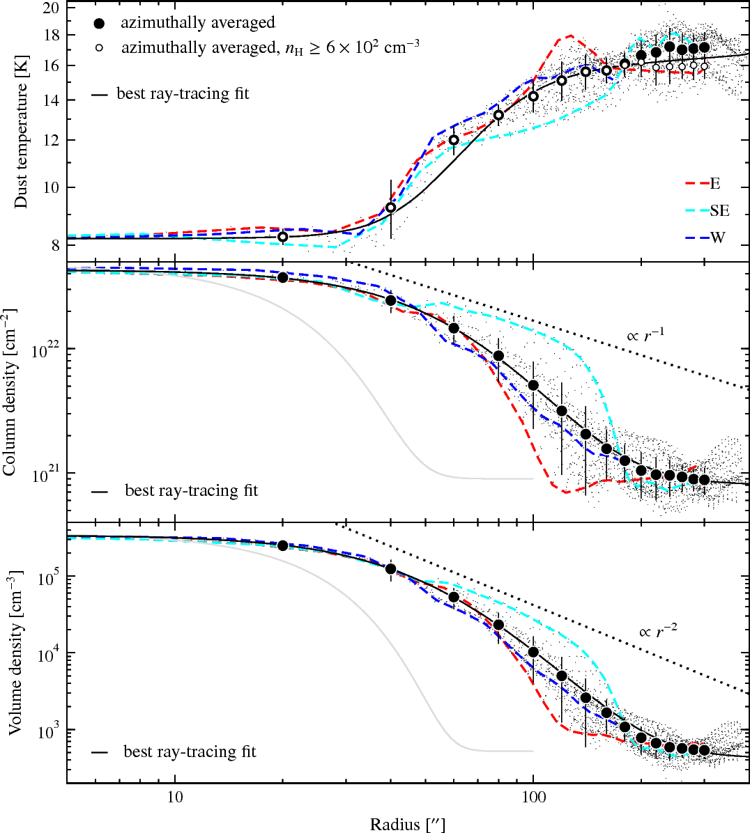
Figure 9: Radial profiles of the dust temperature, the column density and the volume density of B68 based on the distributions shown in Fig 8. All values of the three maps are presented by the small dots. The big filled dots represent azimuthally averaged values inside $20\arcsec$ wide annuli. The open white dots in the upper panel show the same for those dust temperatures that are attained at densities above $6\times 10^{2}$ cm^-2. The error bars reflect the $1\sigma$ r.m.s. scatter of the azimuthal averaging and hence indicate the deviation from the spheroid assumption. We show the best ray-tracing fits to the data that were used to calculate the three maps, indicated by the solid lines. The coloured dashed lines correspond to the radial distributions along three selected directions, as outlined in Fig 8 (c). The dotted lines show the canonical density power-laws for self-gravitating isothermal spheres, and the grey curve depicts a Gaussian profile with a $FWHM$ equal to the spatial resolution of the maps.

Figure 9 (upper panel) summarises the radial distribution of the dust temperature. An azimuthal averaging of the data in annuli of $20\arcsec$ is also shown, both for the entire data and restricted to the a region, where the volume density is $n_{\mathrm{H}}\geq 6\times 10^{2}$ cm^-2. The error bars represent the $1\sigma$ r.m.s. scatter of the azimuthal averaging. Based on these measurements, we find a central dust temperature of $T_{0}=(8.2\pm 0.1)$ K. The azimuthally averaged dust temperature at the edge of B68 amounts to $T_{\mathrm{out}}=(17.6\pm 1.0)$ K for the entire data and $T_{\mathrm{out}}=(16.0\pm 1.0)$ K when omitting the tenuous material where $n_{\mathrm{H}}<6\times 10^{2}$ cm^-2. We have added a corresponding radial profile fit according to Eq. 11.

When considering also the systematic uncertainties of the ray-tracing modelling, the central dust temperature was determined to $T_{\mathrm{d}}=(8.2^{+2.1}_{-0.7})$ K, with the errors reflecting both the range of the valid solutions and statistical errors. We emphasise that this is about $4$ K below the dust temperature that we derived from the LoS averaged SED fitting. As a result, the simple SED fitting approach cannot be regarded as a good approximation for the central dust temperature.

Although the largest scatter in the radial dust temperature distribution of the best model is only of the order of $1.2$ K ($1\sigma$), the peak-to-peak variation at the edge of B68 amounts to about 5 K. To illustrate the contribution of various radial paths to the overall temperature distribution, we have added three diagnostic cuts through the maps from the centre to the eastern, the southeastern, and the western directions, indicated in Figs. 8 (c) and 9.

4.4.2 Column density distribution

Figure 8 (b) shows the column density map of B68 derived from the ray-tracing algorithm as described in Sect. 3.2. It was constructed by LoS integration of the volume density (Sect. 4.4.3). The peak of the column density distribution at RA $=17^{\mathrm{h}}22^{\mathrm{m}}38\aas@@fstack{s}9$, Dec $=-23\degr 49\arcmin 52\arcsec$ can be fitted by a 2D Gaussian with an $FWHM$ of $(87\pm 1)\arcsec\times(76\pm 1)\arcsec$, i.e. about twice the beam size.

The radial column density distribution is presented in Fig. 9 (central panel). It visualises the map values transformed into a radial projection relative to the density peak as well as, azimuthal averages within radial bins of $20\arcsec$. When considering the overall modelling uncertainties as shown in Fig. 7, the central column density amounts to $N_{\mathrm{H}}=(4.3^{+1.4}_{-2.8})\times 10^{22}$ cm^-2, while we find $N_{\mathrm{H}}=(8.2^{+2.3}_{-1.0})\times 10^{20}$ cm^-2 at the edge of the distribution.

The radial profile is also consistent with a relation according to

$$N_{\mathrm{H}}(r)=\frac{N_{\mathrm{H},0}}{1+\left(\frac{r}{r_{0}}\right)^{\alpha}}\quad,$$ (15)

which has the same properties as Eq. 7, but with a different parametrisation (see also Eq. 16). When restricting the fit to $r\leq 200\arcsec$, i.e. before the column density flattens out into the background value, we obtain $r_{0}=45\arcsec$ and $\alpha=2.5$.

Using the method proposed by Tassis & Yorke (2011), the derived column density corresponds to a central hydrogen particle density of $n_{\mathrm{H}}=4.7\times 10^{5}$ cm^-3 with $r_{90}=2505$ AU, which is about 40% above the value we derive from the modelling (see Sect. 4.4.3).

As already described in Sect. 4.4.1, we added three radial cuts through the maps to the profile plots in Fig. 9. They include the most extreme column density variations for the most part of the radial profile, although they are all closely confined to the mean distribution up to an angular radius of $40\arcsec$, whose seemingly very good approximation to a spherical symmetry is owed to a poor sampling of the distribution and beam convolution effects. From here, the eastern cut through the column density drops more quickly than the globule average with $r^{-5.4}$ between radii of $75\arcsec$ and $120\arcsec$, before it reaches the common background value. At approximately $r=50\arcsec$, the southeastern trunk attains a column density plateau at $N_{\mathrm{H}}=2.2\times 10^{22}$ cm^-2, from which it declines with $r^{-0.9}$ to a distance of $90\arcsec$ from the density peak. Finally, it steeply drops with $r^{-9.3}$ between radii of $150\arcsec$ and $190\arcsec$, where it levels out with the background column density.

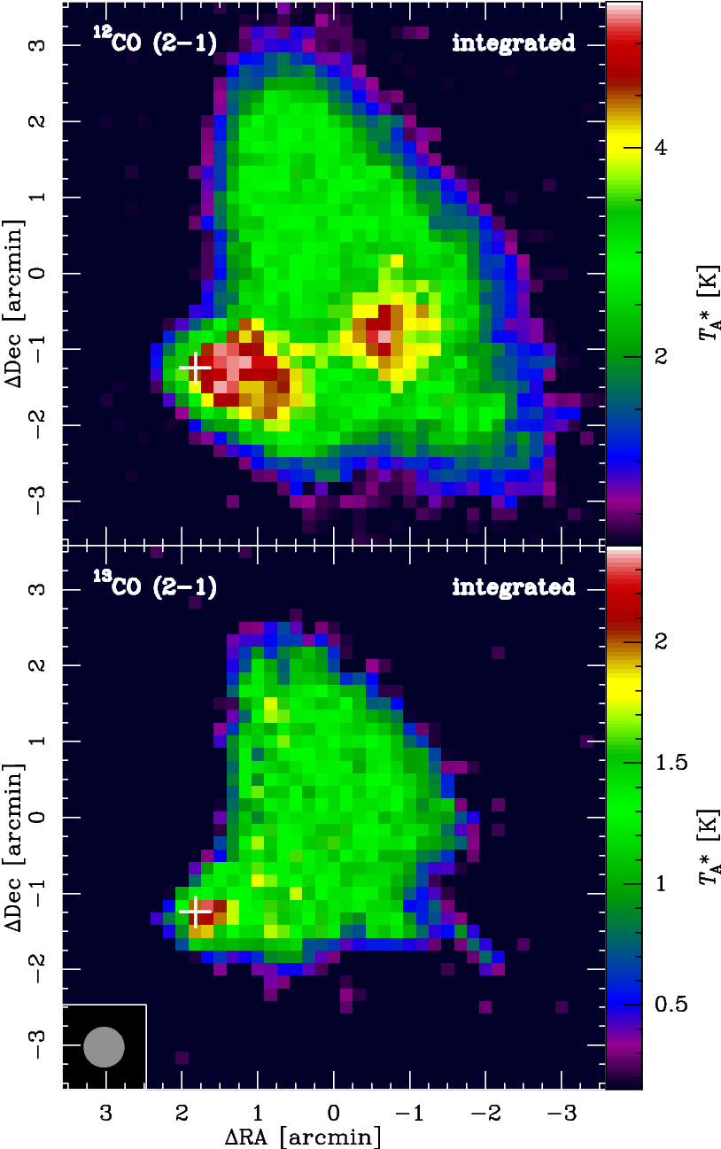
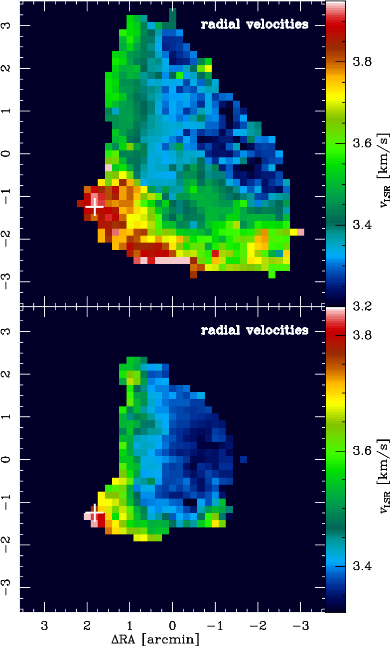
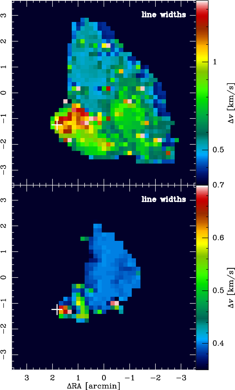
Figure 10: Maps of B68 generated from the CO data. The upper row contains the $\@element[12]{\mathrm{CO}}$ (2–1) line data, while the lower row shows the $\@element[13]{\mathrm{CO}}$ (2–1) observations. The columns from left to right indicate the line flux integrated over all spectrometer channels, the radial velocity distribution, and the corresponding line widths. The white crosses indicate the position of the point source at the tip of the trunk.

The column density map can be used to derive a mass estimate for B68. When including all the data in the column density map, which cover an area of $60\squareforqed\arcmin$, we derive a total mass of $4.2\leavevmode\nobreak\ M_{\sun}$. For the material that represents $A_{K}\geq 0.2$ mag, we get a total mass of $3.1\leavevmode\nobreak\ M_{\sun}$. This value is in good agreement with the one given in Alves et al. (2001b) after correcting for the different assumed distance. In general, the uncertainty on the mass estimate from the modelling alone is rather small ($\pm 0.5\leavevmode\nobreak\ M_{\sun}$), because the various solutions more or less only redistribute the material instead of changing the total amount of mass significantly. We are aware that the uncertainties due to the dust properties are much greater, but they do not change the consistency between the different solutions. That the mass derived from the best ray-tracing fit to the data actually coincides well with the one extracted independently from the extinction mapping is reassuring and demonstrates that the quoted uncertainties are conservative.

4.4.3 Volume density distribution

Figure 8 (c) shows the volume density distribution across the PoS and in the mid-plane along the LoS through of B68 derived from the ray-tracing algorithm described in Sect. 3.2, so it is only the mid-plane slice of the entire ray-tracing cube-fitting result. The peak of the volume density distribution RA $=17^{\mathrm{h}}22^{\mathrm{m}}38\aas@@fstack{s}5$, Dec $=-23\degr 49\arcmin 50\arcsec$ can be fitted by a 2D Gaussian with an $FWHM$ of $(66\pm 1)\arcsec\times(61\pm 1)\arcsec$, i.e. just below twice the beam size.

We show the resulting radial volume density distribution in Fig. 9 (lower panel). Azimuthal averages are added, whose error bars indicate the rms noise of the averaging. The best fit to the data according to Eq. 8 is listed in Table 3. With Eq. 10, we obtain $r_{1}=180\arcsec$ for the LoS profile. The fit is parametrised by $n_{0}=3.4\times 10^{5}$ cm^-3, $r_{0}=35\arcsec$, and $\eta=4.0$. Including the overall conservative ray-tracing uncertainty (Fig. 7), the central volume density amounts to $n_{\mathrm{H}}=(3.4^{+0.9}_{-2.5})\times 10^{5}$ cm^-3. The volume density of the constant background level is modelled as $n_{\mathrm{H}}=(4.4^{+1.8}_{-1.5})\times 10^{2}$ cm^-3.

Similar to Eqs. 15 and 16, the radial distribution can also be fitted with a combination of a flat centre and a power-law at large radii. The resulting fit is not unique and covers a range of fit parameters with $r_{0}=35\arcsec-40\arcsec$ and $\alpha=3.4-3.7$, when restricting the fit to $r\leq 190\arcsec$.

The resulting mid-plane volume density distribution for the selected three directions are also shown. Up to a distance of $1\arcmin$ from the density peak, all profiles agree very well, but deviate in the transition between the flat central profile and the decline towards the edge of the globule. As for the column density distribution, the reduced data sampling and beam convolution effects can contribute to the seemingly good agreement with a spherical geometry in the centre of B68. While the average density profile drops, as shown, approximately with $r^{-3.5}$, the distribution to the eastern edge falls off more sharply, i.e. with $r^{-6.5}$ between $r=75\arcsec$ and $120\arcsec$. The previously reported behaviour of the southeastern trail along the trunk is also reflected in the volume density that reaches a plateau of $n_{\mathrm{H}}=9\times 10^{4}$ cm^-3 between $50\arcsec$ and $70\arcsec$ away from the peak. Then it declines up to $r=90\arcsec$ with $r^{-1.8}$, from which it steeply drops with $r^{-2.7}$ up to a radius of $130\arcsec$, and then with $r^{-10.2}$ between radii of $150$ and $190\arcsec$.

This analysis shows that, although the mean volume density profile is consistent with a spherical 1D symmetry in the centre of the globule, where the density profile is very shallow, that symmetry is broken below densities of $n_{\mathrm{H}}=10^{5}$ cm^-3 and beyond $r\approx 40\arcsec$ (6000 AU at a distance of 150 pc). The largest deviations are seen between the western and southeastern directions, where the volume densities differ by a factor of four at a distance of $90\arcsec$ from the density peak and attain a maximum of factor 20 at $r=120\arcsec$. But even if the peculiar southeastern trunk is not included, we find density deviations between different radial vectors of a factor of 2 at $90\arcsec$ to a factor of 5 at $120\arcsec$.

4.5 CO data

We have mapped the larger area around B68 in the $\@element[12]{\mathrm{CO}}$ (2–1) and the $\@element[13]{\mathrm{CO}}$ (2–1) lines. The resulting integrated line, radial velocity, and line width maps are shown in Fig. 10. Keeping in mind that particularly the centre of B68 is strongly affected by CO gas depletion (e.g.  Bergin et al. 2002), the global shape resembles the known morphology quite well. We see two maxima in the $\@element[12]{\mathrm{CO}}$ (2–1) integrated line maps, while only one peak is visible in the optically thinner $\@element[13]{\mathrm{CO}}$ (2–1) line maps. Interestingly, it coincides with the local maximum at the tip of the southeastern extension of the extinction map of (Alves et al. 2001a) and the source we discovered at 160 and 250 $\mu$m.

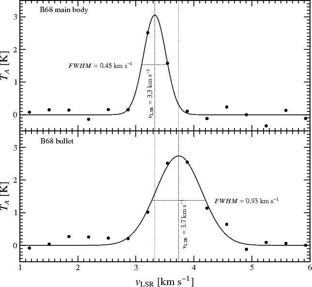
Figure 20: $\@element[13]{\mathrm{CO}}$ (2–1) spectra extracted at two positions in the corresponding map. The upper spectrum shows a line on the western rim of B68 (RA (J2000) = $17^{\rm h}22^{\rm m}34\aas@@fstack{s}1$, Dec (J2000) = $-23^{\circ}49^{\prime}53^{\prime\prime}$), while the lower spectrum is taken at the location of the point source mentioned in Sect. 4.2 A Gaussian profile fit was applied to both spectra.

We confirm a global radial velocity gradient with slightly increasing values from the northwest to the southeast that have been reported by others (e.g.  Lada et al. 2003; Redman et al. 2006) and may indicate a slow global rotation or shear movements. The line widths are rather small and in most cases cannot be resolved by our observations. Strikingly, the highest redshifts and largest apparent line widths are observed towards the aforementioned peak at the tip of the extension, identified as a point source in Sect. 4.2. To investigate this phenomenon closer, we have extracted $\@element[13]{\mathrm{CO}}$ (2–1) spectra at that position and, for comparison, one at the western edge of B68 (available as online material, Fig. 20).

The spectrum taken at the position of the point source is shifted by 0.4 km s^-1, which corresponds to the spectral resolution of the data, and broadened by approximately the same amount. A significant local increase in the temperature can be ruled out by the dust temperature maps and the low colour temperature extracted from the photometry in the Herschel maps, so that a line broadening due to thermal effects seems unlikely, at least at the spectral resolution obtained with our data. Instead, it can be explained by a superposition of two neighbouring radial velocities ($\sim 3.3$ and $\sim 3.7$ km s^-1). This interpretation is supported by already published spectral line observations at higher spectral resolution that reveal a double-peaked line shape (e.g.  Lada et al. 2003; Redman et al. 2006).

5 Discussions

5.1 Temperature and density

5.1.1 The temperature distribution

In Sect. 4.4.1, we have presented the results of the dust temperature distribution of B68. At the resolution of the SPIRE 500 $\mu$m data ($36\aas@@fstack{\prime\prime}4$), the central dust temperature was determined to $(8.2{+2.1\above 0.0pt-0.7})$ K, considering the uncertainties of the ray-tracing modelling algorithm (see Sect. 3.2). The temperature at the edge of B68 including volume densities below $6\times 10^{2}$ cm^-3 was measured to 16.7 K with an uncertainty of $\pm 1$ K. When considering only material that is denser than this value, the outer dust temperature is $0.7$ K lower, which results in an edge-to-core temperature ratio of $2.0$.

Model calculations using radiative transfer towards idealised isolated 1D BES of similar densities show central temperatures of the order of $7.5$ K and higher (Zucconi et al. 2001) which confirms our result. Modifying the BE approach to a non-isothermal configuration does not change the situation significantly (Sipilä et al. 2011). The coldest prestellar cores found to date populate a temperature range around 6 K, but also possess densities and masses higher than B68 (e.g.  Pagani et al. 2004; Doty et al. 2005; Crapsi et al. 2007; Pagani et al. 2007; Stutz et al. 2009).

Previous estimates of the dust temperature in B68 lacked either the necessary spectral or spatial coverage and quote mean values around 10 K for the entire core (e.g.  Kirk et al. 2007). In addition, Bianchi et al. (2003) were able to deduce a deviation from the isothermal temperature distribution by analysing (sub)mm data. They derived an external dust temperature of $14\pm 2$ K, which, in the absence of higher frequency data, tends to underestimate the real value. Nevertheless, it is consistent with our results when discarding the warmer low-density regime.

Determining the central gas temperature and its radial profile turned out be more successful (e.g.  Hotzel et al. 2002a; Bergin et al. 2006), and generally one would expect both the gas and the dust temperature to be tightly coupled in the core centre, where they experience densities of $n_{\mathrm{H}}\geq 10^{5}$ cm^-3 (e.g.  Lesaffre et al. 2005; Zhilkin et al. 2009), with the strength of the coupling gradually increasing already from $n_{\mathrm{H}}\approx 10^{4}$ cm^-3 (Goldsmith 2001). However, Bergin et al. (2006) found evidence that this might not be necessarily the case. They have reconstructed the dust temperature profile by chemical and radiative transfer modelling of CO observations (their Fig. 2a) and also predict a central value of $\approx 7.5$ K, which is significantly below what they find for the central gas temperature. Their results even revealed a gas temperature decrease to larger radii, which is confirmed by Juvela & Ysard (2011) in a more generalised modelling programme. They demonstrate that the gas temperature in dense cores can be affected by many contributions and thus alter the central temperature by up to 2 K, depending on the composition of the various physical conditions. This can lead to diverging gas and dust temperatures in the centre of dense cores (e.g.  Zhilkin et al. 2009). According to Bergin et al. (2006), this can only be explained by a reduced gas-to-dust coupling in the centre of B68, especially when – as in this case – the gas is strongly depleted.

Figure 11: $N_{\mathrm{H}}$ vs. $A_{K}$ ratio map. The uncertainties increase strongly beyond a radius of $180^{\prime\prime}$, because a) the flux densities and extinction values are low towards the southeast, b) the extinction map has a higher uncertainty there, c) edge effects in the modelled flux distribution. The position of the embedded point source is indicated with a white cross.

5.1.2 The density distribution

In Sect. 4.4.2, we have described and analysed the column density distribution that we derived from the ray-tracing modelling. It peaks at $N_{\mathrm{H}}=(4.3{+1.4\above 0.0pt-2.8})\times 10^{22}$ cm^-2 towards the centre of B68 and blends in with the ambient medium of $N_{\mathrm{H}}=(8.2^{+2.3}_{-1.0})\times 10^{20}$ cm^-2 at $\approx 200\arcsec$. The central value is in good agreement with the results of Hotzel et al. (2002a). Further investigations led them to the conclusion that the gas-to-dust ratio in B68 is below average, i.e. also less than our assumption made for the modelling. The actual column density may thus be lower.

Since we have two independent measurements of the column density, the extinction and the emission data, we can compare both and test how consistent they are. For this purpose, we first analysed a possible variation in the ratio between the $N_{\mathrm{H}}$ and $A_{K}$ maps. A ratio map is shown in Fig. 11. The strong drop towards the southeast is very uncertain due to higher uncertainties in the extinction and the modelled column density maps. Therefore, we only consider the area up to $r=180^{\prime\prime}$. Within this range, the mean value is $N_{\mathrm{H}}/A_{K}=1.3\times 10^{22}$ cm^-2 mag^-1. The ratios at the centre of B68 appear slightly increased when compared to the rest of the globule. An azimuthally averaged radial profile up to $r=180^{\prime\prime}$ is presented in Fig. 12 (upper panel). The variation amounts to 12% around the mean value. We also plot the relationships found by Vuong et al. (2003) and Martin et al. (2012). In fact, the latter work presents a conversion between $N_{\mathrm{H}}$ and $E_{J-K}$, which is based on a linear fit to data points with a significant amount of scatter. In addition, those data only covered extinctions up to $A_{V}\approx 3$ mag. Nevertheless, when applying the extinction law of Cardelli et al. (1989), we find $N_{\mathrm{H}}/A_{K}=1.7\times 10^{22}$cm^-2mag^-1.

Vuong et al. (2003) derive values in the $\rho$ Oph cloud using two different assumptions of the metallicity that sensitively modify the extinction determined from their X-ray measurements. The corresponding values for the $N_{\rm H}/A_{K}$ ratio differ by almost 30%. They range between $1.4\times 10^{22}$cm^-2mag^-1 for standard ISM abundances and $1.8\times 10^{22}$cm^-2mag^-1 for a revised metallicity of the solar neighbourhood (Holweger 2001; Allende Prieto et al. 2001, 2002), which is apparently closer to the mean value of the Galaxy, if $R_{V}=3.1$ is assumed. However, one should probably not even expect a good agreement considering the different LoS towards the Ophiuchus region and the Galactic centre. In Fig. 12, the value for the standard ISM abundances is in remarkably good agreement with our analysis, although the alternative ratios still fit reasonably well, considering the large uncertainties.

Figure 12: Radial profiles of the $N_{\mathrm{H,mod}}/A_{K}$ ratio (upper panel) and the $N_{\mathrm{H}}$ ratio between the modelled column density and the one derived from the NIR extinction for three values of $R_{V}$ (lower panel). The $N_{\mathrm{H,mod}}/A_{K}$ ratio attains a mean value of $1.3\times 10^{22}$ cm^-2 mag^-1 with a scatter of 12%. This corroborates the estimate of Vuong et al. (2003) using the standard metallicity of the ISM. A good agreement between the modelled column density and the one based on the extinction is achieved for a slightly increased $R_{V}$ value of about 4.

For a suitable conversion from $A_{K}$ to $N_{\mathrm{H}}$, we can also compare ratios of the column densities derived from the modelling and the extinction map directly. Vuong et al. (2003) have already discussed the possibility that their apparent mismatch of the $N_{\mathrm{H}}/A_{J}$ ratio with the galactic mean value may not be related to a difference in metallicities, but more a variation of the $R_{V}$ value from the one of the diffuse ISM. They refer to a previous estimate of $R_{V}=4.1$ in the outskirts of the $\rho$ Oph cloud (Vrba et al. 1993). In general, increased $R_{V}$ values are common in dense regions (e.g. Chini & Krügel 1983; Whittet 1992; Krügel 2003; Chapman et al. 2009; Olofsson & Olofsson 2010). Therefore, we chose to apply a conversion via $A_{V}$ by assuming the extinction law of Cardelli et al. (1989) and a given value of $R_{V}$.

Recent conversions between $A_{V}$ and $N_{\mathrm{H}}$ are determined for the diffuse ISM that on average attains $R_{V}=3.1$. For such an assumption, we can use $2.2\times 10^{21}$ cm^-2 mag^-1 (Ryter 1996; Güver & Özel 2009; Watson 2011). We can then derive modified conversions for varying values of $R_{V}$, which in our analysis was iterated between 3.1, 4.0, and 5.0. The corresponding column density ratios between the modelled distribution and the one derived from the extinction are shown in Fig. 12 (lower panel). A reasonable agreement is only reached for a slightly increased $R_{V}$ value around 4, which is in excellent agreement with the value obtained by Vrba et al. (1993). A change in $R_{V}$ is usually attributed to an anomalous grain size distribution (e.g.  Román-Zúñiga et al. 2007; Mazzei & Barbaro 2008; Fitzpatrick & Massa 2009), which would be consistent with the interpretation of Bergin et al. (2006) for a reduced gas-to-dust coupling rate. While the result of an increased $R_{V}$ relative to the canonical $R_{V}=3.1$ in the diffuse ISM may point to the possible presence of grain growth processes in B68, systematic uncertainties in the modelling could affect the derived $R_{V}=4$ value. Therefore this result should be interpreted with caution.

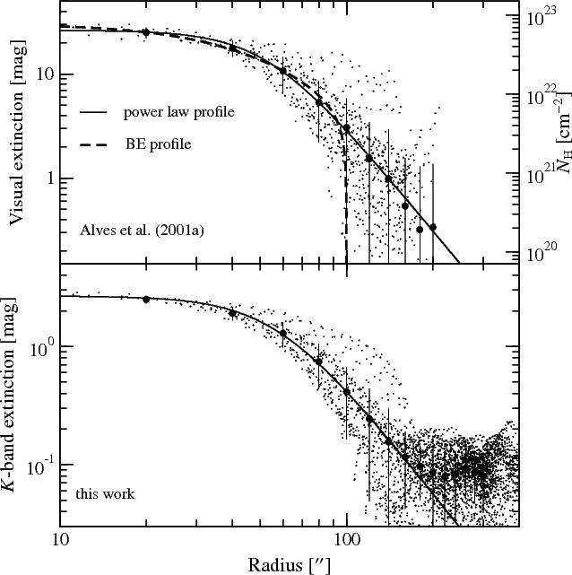
Figure 21: Radial profiles extracted from the extinction map of Alves et al. (2001a) (upper panel) and the newly calculated extinction map shown in Fig. 2 (lower panel). The small dots represent the data in the maps after regridding them to the same scale; the large dots are the mean values in bins of $20\arcsec$ each with the error bars indicating the corresponding r.m.s. scatter. The mean distributions follow a profile fit similar to Eq. 15 (solid line). The power-law indices are $\alpha=3.3$ in the upper panel and $\alpha=3.1$ in the lower panel. For comparison, we added the profile of the BES (dashed line) given by Alves et al. (2001b).

The radial distribution of column densities or extinction values of prestellar cores is often modelled to represent a BES. For B68, this was done by Alves et al. (2001b), who were able to fit a BE profile with an outer radius of $100^{\prime\prime}$ (see Fig. 21, available as online material). A quick investigation demonstrates that power-law profiles according to Eqs. 7 and 15 with a wide variety of parameters fit the radial distribution up to $r=60^{\prime\prime}$ equally well. However, the derived BE profile fails to match the column density distribution between radii of $100^{\prime\prime}$ and $200^{\prime\prime}$. This does not mean that no BES model fits the full column density profile of B68, but at least the one derived by Alves et al. (2001b) cannot account for the extended distribution shown in Figs. 9 and 21. In contrast, the profiles we use to characterise the radial distributions fulfil this requirement. They are even very similar for the two radial extinction profiles we show in Fig. 21, which indicates that, within the mutually covered area, the revised extinction map (Fig. 2) agrees well with the one of Alves et al. (2001a).

Section 4.4.3 presents our ray-tracing modelling results of the volume density distribution in the mid-plane of B68, i.e. traced across the PoS at a position half way through the globule. We find a central particle density of $n_{\mathrm{H}}=(3.4{+0.9\above 0.0pt-2.5})\leavevmode\nobreak\ \times 10^{5}$ cm^-3, while it drops to $n_{\mathrm{H}}=(4.4{+1.8\above 0.0pt-1.5})\leavevmode\nobreak\ \times 10^{2}$ cm^-3 at the background level. That the resulting mass range of $3.1-4.2\leavevmode\nobreak\ M_{\sun}$ for an assumed distance of 150 pc is in good agreement with the previous independent estimates puts the valid density range into a different perspective and demonstrates that assumed uncertainties are rather conservative.

The central density is a factor of $0.4$ below what we estimate by applying the simplified method of Tassis & Yorke (2011), but it is consistent with the result of Dapp & Basu (2009). Tassis & Yorke (2011) expect the deviations in the results derived with their method to be within a factor of two of the real value, and Dapp & Basu (2009) assume a temperature of $11$ K for the entire core. Thus, considering the uncertainties, their results are in reasonably good agreement with our analysis.

The theoretical model of inside-out collapse of prestellar cores predicts a density profile of $n_{\mathrm{H}}\propto r^{-2}$ (e.g.  Shu 1977; Shu et al. 1987), which appears to be present in most of the cores observed to date (e.g.  André et al. 1996). Nevertheless, steeper profiles have been reported as well (e.g.  Abergel et al. 1996; Bacmann et al. 2000; Whitworth & Ward-Thompson 2001; Langer & Willacy 2001; Johnstone et al. 2003). As mentioned in Sect. 4.4.3, we also find a rather steep power-law relation for the mean profile and most of the radial cuts through the density map of the order of $n_{\mathrm{H}}\propto r^{-3.5}$. It is consistent with the relation we find for the column density, whose slope follows a power law of $N_{\mathrm{H}}\propto r^{-2.5}$. Bacmann et al. (2000) show that the simple relation $N_{\mathrm{H}}\propto r^{-m}\Leftrightarrow n_{\mathrm{H}}\propto r^{-(m+1)}$ (e.g.  Adams 1991; Yun & Clemens 1991) does not hold for a more realistic description by piecewise power-laws. For large radii, the difference of the two slopes is reduced to $\approx 0.6$. That the revised extinction map (Fig. 2) shows similar power-law behaviour of the form $A_{K}\propto r^{-3.1}$ for $60\arcsec\leq r\leq 180\arcsec$ (available as online material, Fig. 21) independently confirms our result. In addition, we confirm this finding with the better resolved NIR extinction map of Alves et al. (2001a), although the area covered with these data is considerably smaller (available as online material, Fig. 21). This demonstrates that resolution effects are negligible in this aspect.

To be able to evaluate possible physical reasons for such steep slopes, we first have to discuss contributions that result from the observing strategy and the data handling. Our ray-tracing approach produces a volume density map that relies on the profile fitting of the first estimate of the column density distribution we get from the SED fitting. Therefore, any modification introduced by technical and procedural contributions affects the column density distribution first and then propagates through to the modelled volume density. Since the profiles derived across the PoS are used to parametrise the behaviour along the LoS, they have a direct impact on the ray-tracing results for the volume density distribution as well. To find non-physical reasons for the steep volume density profiles, we must therefore take one step backward and have a look at the equally steep column density profiles.

One contribution comes from resolution effects. To test their influence on the radial profiles, we performed 1D radiative transfer calculations of a model core with a flat inner density distribution that turns over into $n_{\mathrm{H}}\propto r^{-2}$ behaviour towards the edge. At large radii, the resulting column density profile possesses a relation $N_{\mathrm{H}}\propto r^{-1.4}$ due to LoS projection effects, as already shown by Bacmann et al. (2000). After convolving this configuration with a beam of $37\arcsec$, the $r^{-1.4}$ relation has migrated to smaller radii, simulating a steeper slope in the inner parts of the core. In combination with the flattening of the core centre, this produces the impression of a relative strong turnaround from a rather flat to a steep slope at intermediate core radii. However, this effect cannot change the steepness of the slopes. As a result, it cannot explain the steep $N_{\mathrm{H}}\propto r^{-2.5}$ behaviour beyond $r\approx 60\arcsec$, unless the actual profile reaches such a slope anywhere along the observed radii. We emphasise that this effect is not unique to the data used in this investigation, and to some degree all observations suffer from this effect, depending on the spatial resolution. If it were responsible for the observed steepness, we should expect to see a relation of the observed slope with resolving power. Already the moderately convolved ($10\arcsec$) extinction data of Alves et al. (2001b) produce a mean radial profile whose slope is nearly indistinguishable from the one of the column density profile shown in Fig. 9 (cf. Sect. 5.1.2), so, the more than three times worse resolution does not change the situation significantly.

Another reason for the steepness of the mean radial profile is the asymmetry of B68 that can be best judged by the profiles of the three cuts through the density map. In particular, the path towards the east drops much more quickly than others, which points to a smaller extent in this direction. Such parts reduce the azimuthal averages, which leads to a faster decline of the mean radial profile in relation to one that belongs to a symmetric core. This also means that for asymmetric cores – and most cores are like that – an azimuthally averaged radial profile is of limited value, especially at large distances from the core centre. Instead, a proper 3D treatment is needed to actually infer realistic physical core properties. This will be attempted in a forthcoming paper.

Nevertheless, Fig. 9 demonstrates that most data follow the same power-law as the mean profile which means that for the majority of the core radii, the density does behave like $n_{\mathrm{H}}\propto r^{-3}$. Interestingly, only the cut following the southeastern trunk is close to the theoretically predicted $N_{\mathrm{H}}\propto r^{-1}$ and $n_{\mathrm{H}}\propto r^{-2}$ relations.

An artificial offset in the density can also modify the slope of a power law. If, for instance, we add a constant density of $10^{4}$ cm^-3, the mean radial profile attains a $n_{\mathrm{H}}\propto r^{-2}$ power-law for $60\arcsec\leq r\leq 120\arcsec$. However, it is difficult to imagine how such an offset could be introduced by the SED fitting and the modelling via the ray-tracing algorithm.

In Fig. 13, we demonstrate the influence of three different modelling approaches on the resulting column density estimate for B68. The simplest way to constrain the temperature is to assume a constant value for the entire core, as has been done many times before. This unrealistic assumption of isothermality apparently tends to produce an extremely broad, flat central density distribution at a relatively low column density estimate. In the current example of $T_{\mathrm{d}}=15$ K, the central column density estimate is only half of the ray-tracing result. The modified black body fit approach mitigates this disadvantage to some extent, but still underestimates the central density owing to the already discussed LoS averaging effect. Another clear difference is the slope of the intermediate region between the core centre and its edge. Fitting the transition region around $r=100\arcsec$ by $N_{\mathrm{H}}=N_{0}r^{-\alpha}$, we find $\alpha=1.6$ for the isothermal case, but $\alpha\approx 2.4$ for the SED fitting and the ray-tracing approaches. However, fitting Eq. 15 yields $\alpha\approx 2.5$ for all three radial distributions, with considerable differences of the turnaround radius $r_{0}$ ranging from $87\arcsec$ for the isothermal case via $55\arcsec$ for the modified black body fit to $45\arcsec$ for the ray-tracing. This demonstrates that apparently a simple description via $N_{\mathrm{H}}=N_{0}r^{-\alpha}$ can be misleading, if the ratio between the calculated width of the inner core and the total core size is too large, as it is obviously the case for the isothermal assumption. In other words, the turnaround has not fully progressed yet, before the profile slowly fades out into the tenuous density of the background or halo. In such situations, it is difficult if not impossible to actually identify a range of constant decline.

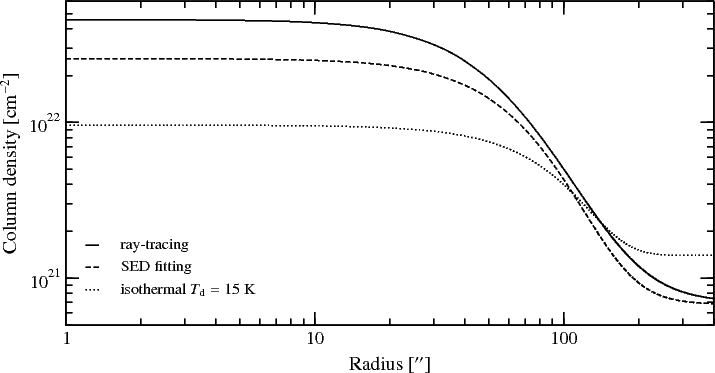
Figure 13: Comparison of radial column density profiles for three different approaches of confining the dust temperature.

Since the ray-tracing modelling produces a range of valid power-law slopes (Fig. 7) between $\alpha=3.1$ and $4.5$, the actual value may be uncertain. Nevertheless, it appears justified to conclude that $\alpha>3$ and therefore the slope we find in the ray-tracing data is clearly steeper than $\alpha=2$. For this reason, it is legitimate to look for physical reasons for this phenomenon. André et al. (2000) point out that isolated prestellar cores appear to have sharp edges with density gradients steeper than $n_{\mathrm{H}}\propto r^{-3}$ for $r\ga 15\,000$ AU, i.e. in this case $100\arcsec$, that could be explained by a core in thermal and mechanical equilibrium interacting with an external UV radiation field, if the models of Falgarone & Puget (1985) and Chièze & Pineau Des Forêts (1987) are considered. Whitworth & Ward-Thompson (2001) have picked up that statement and derived an empirical, non-magnetic model for prestellar cores that follows a Plummer-like density profile (Eq. 7) with $\eta=4$. Strikingly, we find exactly the same value in our LoS profile fit.

Interestingly, Eq. 7 with $\eta=4$ is analytically almost identical to the theoretical density profile of an isothermal, non-magnetic cylinder (Ostriker 1964). This concept was observationally confirmed by Johnstone et al. (2003), who find density profiles steeper than $r^{-3}$ for several sections in the filament of GAL~011.11-0.12. The relevance to the case B68 is the conjecture that it belongs to a chain of individual globules that once formed as fragments of a filament that has meanwhile been dispersed. Figure 1 illustrates this view, where several cores appear aligned along a curved line. In addition, there is B72 to the north of the image that is still embedded in a tenuous filament. It is conceivable that the remaining fragments still contain an imprint of the density profiles of the former filament. In that case, the other globules of that chain should also possess steep profiles, just like B68. If this scenario is true, B68 might not be the prototypical isolated prestellar core as often suggested. This idea plays a central role in the concept of colliding cores we discuss in Sect. 5.3.

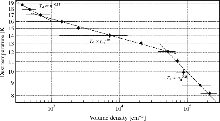
Figure 14: Dust temperature profile as a function of volume density $n_{\mathrm{H}}$. The error bars indicate the r.m.s. scatter of the averaging inside the individual bins. The relation can be distinguished into three regions.

To visualise the relation between the resulting dust temperature and volume density distributions, we have produced a temperature averaged density profile (Fig. 14). The relation can be distinguished into three sections with $T_{\mathrm{d}}\propto n_{\mathrm{H}}^{\beta}$, where

$$\beta=\left\{\begin{array}[]{ll}-0.15&\quad\textrm{for \quad$n_{\mathrm{H}}<10^{3}$\leavevmode\nobreak\ cm${}^{-3}$}\\ -0.08&\quad\textrm{for \quad$3\times 10^{4}$\leavevmode\nobreak\ cm${}^{-3}>n_{\mathrm{H}}\geq 10^{3}$\leavevmode\nobreak\ cm${}^{-3}$}\\ -0.28&\quad\textrm{for \quad$n_{\mathrm{H}}>6\times 10^{4}$\leavevmode\nobreak\ cm${}^{-3}$}\quad.\end{array}\right.$$

We interpret this behaviour as a result of the different heating and cooling effects that are influencing the temperature and density structure of B68. Even for relatively dense cores, the heating by the external ISRF is the dominating contribution (Evans et al. 2001). Only the effective spectral composition changes with the density of the core material. At the tenuous surface, heating by UV radiation can be non-negligible, which leads to a higher heating efficiency. At densities above $10^{3}$ cm^-3, heating by UV radiation is shut off. The IR and mm radiation of the ISRF as well as cosmic rays with their secondary effects, remain as the only heat sources. This leads to a shallower relation between the dust temperature and the density. At densities $10^{4}$ cm${}^{-3}<n_{\mathrm{H}}<10^{5}$ cm^-3, gas and dust begin to couple, which coincides with the turnaround to a steeper relationship. This range corresponds to small radii, so that beam smearing effects contribute to the slope measured in the data. The actual behaviour may be different.

5.2 Anisotropic interstellar radiation field

The ISRF at the location of B68 heating the dust particles is unknown. We expect it to be strongly anisotropic and wavelength-dependent as revealed e.g. by the all-sky surveys like the Diffuse InfraRed Background Experiment (DIRBE) at solar location. Such an anisotropic irradiation can cause surface effects on isolated globules like B68 and may explain the crescent structure discovered with the Herschel observations at 100 and 160 $\mu$m. Since this also implies an anisotropy in the heating, the discovery of a sudden rise of the dust temperature at the southeastern rim, as described in Sect. 4.3, may be another result of the ISRF geometry. As shown by Fig. 15, this side faces the galactic plane at a latitude of about 7$\aas@@fstack{\circ}$1. For an altitude of the sun of 20.5 pc above the galactic plane (Humphreys & Larsen 1995), the galactic altitude is approximately 40 pc for B68. This suggests that the local radiation field of the Milky Way may heat B68 from behind, but at some degree also from below. With respect to dust heating, its contribution can be divided into two parts.

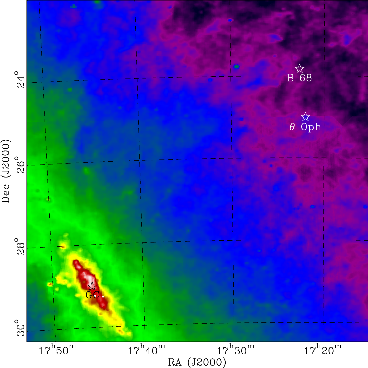
Figure 15: IRAS map at $\lambda=60\leavevmode\nobreak\ \mu$m covering the galactic plane and B68. North is up and east is left. B68 is located 7$\aas@@fstack{\circ}$1 above the galactic plane. At a distance of 150 pc, this translates to a galactic altitude of 40 pc. The position of the B2IV star $θ$~Oph is also indicated. Its parallax of $\pi=7.48\pm 0.17$ mas (van Leeuwen 2007) puts it at a distance of 134 pc. Its distance to B68 is approximately 20 pc.

At longer wavelengths, the SED of the Milky Way peaks around 100 $\mu$m that varies only with galacto-centric distance (e.g.  Mathis et al. 1983), aside from the 2.7 K cosmic background contribution. The dust opacities are low enough at FIR wavelengths to keep low-mass cores like B68 transparent. For grain heating calculations, the anisotropy in the FIR ISRF can therefore be ignored.

At shorter wavelengths, several effects make the prediction of the local B68 ISRF and its heating more difficult. The stellar radiation sources create an SED, which requires a superposition of Planck curves when being modelled peaking around $1\leavevmode\nobreak\ \mu$m, all showing spatial variations. Since the optical depth at these wavelengths becomes comparable to or greater than one for many lines-of-sights in the Milky Way, the absorbed energy can strongly vary even for neighbouring cores, depending on their relative positions with respect, e.g., to the Galactic centre. Furthermore, scattering becomes important and adds a diffuse component that heats shielded regions. Finally, outer diffuse cloud material surrounding most molecular cloud cores can pile up enough dust mass to effectively shield the core from the NIR and MIR radiation.

There are just a few core models that make use of an anisotropic background radiation field. In their study of the core $ρ$~Oph~D, Steinacker et al. (2005b) have used a combination of a mean ISRF given in Black (1994), an MIR power-law distribution as suggested in Zucconi et al. (2001) to account for the nearby photo-dissociation region (PDR), and the radiation field of a nearby B2V star. A similar approach was applied by Nutter et al. (2009) to model LDN 1155C. The anisotropic DIRBE all-sky map at 3.6 $\mu$m was used in Steinacker et al. (2010) to model the core LDN~183 in absorption and scattering.

Figure 16: Results of the 3D modelling showing the influence of heating from an anisotropic ISRF on the FIR emission of a B68-like globule. The upper left panel reflects the column density of the model globule, the lower left panel shows the 100 $\mu$m emission as observed with Herschel. The remaining four images show the modelled FIR maps at 100 (central column) and 160 $\mu$m (right column) for an isotropic (top) and an anisotropic (bottom) ISRF.

In a concept study to investigate, if the strong FIR emission in the part facing the galactic plane and the Galactic centre is caused by an anisotropic illumination of B68, we have constructed a simple model that mimics its basic structural features. The main core body is approximated by a 3D clump with the radial vector R defined by $R^{2}=(x/A)^{2}+(y/B)^{2}+(z/C)^{2}$ and a model dust number density dropping to zero outside $r_{\mathrm{out}}$ following

$$n_{M}(\@vec{x})=\frac{n_{M,0}}{1+\left(\frac{R(\@vec{x})}{R_{0}}\right)^{\alpha}}\quad.$$ (16)

A smaller clump with the same density structure was placed southeast of the main clump to represent the southeastern extension of B68. The clumps do not overlap to avoid density enhancement at the border of the main clump. The assumed masses are 2.5 and $0.25\leavevmode\nobreak\ M_{\sun}$, respectively. With its low mass and off-centre position, it should be heated up easily by the ISRF showing a stronger emission at shorter wavelengths compared to shielded regions near the core centre. Two ISRF illuminations were considered: isotropic illumination by the SED described in Zucconi et al. (2001) and anisotropic illumination approximated by the same SED through a cone with an opening angle of $20\degr$ that is oriented towards the direction of the Galactic centre, where the NIR contribution attains its maximum. Since B68 is located about $7\degr$ above the Galactic centre seen from Earth, this causes a slightly stronger illumination from below. Test calculations with a ray-tracing version of the code described in Steinacker et al. (2003) yielded that considering scattering as a source term in the radiative transfer will only lead to marginal temperature changes in the outer parts of the model core. Since we use only an approximate ISRF and did not consider images at shorter wavelength, we neglected it. We performed radiative transfer calculations including extinction on a grid with $10^{6}$ cells, 600 equally-spaced direction nodes per cell (Steinacker et al. 1996), and 61 wavelengths with simple opacities from Draine & Lee (1984) to compare the results during the code testing with former results obtained with the same opacities.

Figure 17: $\@element[13]{\mathrm{CO}}$ (2–1) channel maps of the molecular line observations of B68. The radial velocities are indicated. The contours superimposed in the upper row and in the left panel of the lower row represent the LABOCA data. The contours in the lower right panel show the extinction map of Alves et al. (2001a). There is a general trend of the radial velocities being somewhat higher towards the eastern edge of B68. The highest velocities at $v_{\mathrm{LSR}}\approx 4.1\pm 0.2$ km s^-1 can be attributed to a point source that coincides with a local density peak at the tip of southeastern extension.

The results are shown in Fig. 16. The upper left-hand image shows the dust column number density $N$ of the two-clump model as an image. The projection of the overlapping clump regions causes a local maximum. Likewise, observed column density maxima or emission maxima at wavelengths where the core is optically thin, can be an effect of projection without number density maxima in the real structure. The middle and right upper images give the theoretical intensity at 100 and 160 $\mu$m for the case of isotropic illumination. In both images the central density peak of the main clump also shows an emission maximum that is not seen in the observed images. For the 100 $\mu$m image, the global emission peak appears in the overlap region of both clumps since the small clump is not shielded but carries about a tenth of the gas mass of the main clump. Even in the case of isotropic illumination, structures outside the main clump will appear in emission at 100 $\mu$m. This wavelength range is sensitive to temperature differences due to the exponentially rising Wien part of the thermal emission. In the 160 $\mu$m image, the effect is less pronounced with the main density peak also showing the strongest emission.

The lower panels show the observed PACS image at 100 $\mu$m, and the simulated images at 100 and 160 $\mu$m for an illumination by an anisotropic ISRF. The outer clump again appears in emission. The 100 $\mu$m image simulated for anisotropic illumination, however, shows stronger emission in the southern parts of the model core with a depression of flux in the central region as seen in the PACS image. The 160 $\mu$m model image still shows more emission in the southern part, but no depression near the column density centre, again in qualitative agreement with the PACS image.

This means that a correct modelling of B68 requires the inclusion of the full anisotropic radiation field and its wavelength dependency, including the contributions from the nearby B2IV star $θ$~Oph which in our calculations accounted for 1% of the full incident radiation field. This is especially important for verifications of the balance between the thermal pressure gradient and the gravitational force that is assumed when modelling B68 as a BES (Steinacker et al. 2005a). An investigation of nearby cores should reveal one-sided heating in the same direction, if the cores of the snake nebula are not shielding each other. This will be the focus of a subsequent publication.

5.3 The core collision scenario

Previous molecular line studies (e.g.  Bergin et al. 2002; Lada et al. 2003; Bergin et al. 2006; Redman et al. 2006; Maret et al. 2007) have revealed a high degree of gas depletion in the centre of B68, as well as a complex radial velocity field that indicates oscillations with lifetimes that are typically longer than the sound crossing time (Lada et al. 2003; Keto et al. 2006; Redman et al. 2006). Nevertheless, other dynamical states like a global infall cannot be ruled out (Keto et al. 2006; Broderick et al. 2007).

An intriguing scenario is suggested by Burkert & Alves (2009), who proposed an explanation for the relative large lifetime of at least $3\times 10^{6}$ yr that is needed to explain the stable oscillations being driven by a subsonic velocity field. They found this to be inconsistent with the suggestion of Alves et al. (2001b) that B68 is gravitationally unstable and collapses with a free-fall timescale that is an order of magnitude smaller. In addition, the gas density and temperature distribution can be best reproduced for an age of some $10^{5}$ yr (Bergin et al. 2006). Burkert & Alves (2009) interpret the local maxima of column density in the southeastern trunk of B68 discovered in the NIR extinction map of Alves et al. (2001a) in terms of a small core of $0.2\leavevmode\nobreak\ M_{\sun}$ colliding with the main body of B68. Based on this assumption, they were able to identify such a collision as a possible trigger that recently pushed B68 beyond the boundary of gravitational instability and initiated the gravitational collapse. Kitsionas & Whitworth (2007) have identified the collision of clumps of ISM as a possible trigger for star formation in a more general way.

We have shown that a density peak appears in the Herschel maps and can be distinguished as a point source. In addition, we discovered at that very location a global maximum in the integrated $\@element[13]{\mathrm{CO}}$ distribution (see Sect. 4.5), whose spectral line is slightly redshifted and broadened relative to the main core of B68. Besides a global velocity gradient from west to east, the individual channel maps of the $\@element[13]{\mathrm{CO}}$ (2–1) observations in Fig. 17 identify a point source that is kinematically separated from the main core. The highest radial velocities are only present in this source. The contours of the LABOCA 870 $\mu$m and the NIR extinction map of Alves et al. (2001a) unambiguously identify this object with the density peak at the tip of the southeastern extension of B68. Interestingly, the second peak, which is located more to the centre of B68 and which appears to have a higher column density (Alves et al. 2001a), remains inconspicuous in our continuum and molecular line maps, but may produce a weak signal in the C¹⁸O (1–0) map of Bergin et al. (2002) and the CS  (2–1) map of Lada et al. (2003).

It is noteworthy that previous molecular line investigations see the global radial velocity gradient (e.g.  Lada et al. 2003), but not the kinematically isolated point source. The reason for this appears to be that either that position was not covered (Lada et al. 2003; Redman et al. 2006) or the velocities at $v_{\rm LSR}\approx 4.1\pm 0.2$ km s^-1 were not included. Nonetheless, we have identified this very object in the C¹⁸O data of Bergin et al. (2002) after our own re-analysis of the underlying observations. This new picture is consistent with the scenario of a low-mass core, also referred to as the “bullet”, colliding with a more massive core as portrayed by Burkert & Alves (2009). They also argue that the chain of cores that include B68 and, to the southeast, B 69 to B 71, may be the remainder of a fragmented filament in which the individual cores move along its direction and eventually merge with each other.

While most molecular line studies were restricted to B68, we have also included the neighbouring southeastern cores of Barnard~69 and Barnard~71 (see Fig. 1) in our CO-observing campaign. Figure 18 shows a radial velocity map of the $\@element[13]{\mathrm{CO}}$ (2–1) line of this area that reveals a large radial velocity gradient from the north to the south, in which B68 is only a part of the larger distribution of velocities. The greater picture therefore indicates that at least some of the radial velocity gradient seen in B68 is not related to a rotation of B68. The $\@element[12]{\mathrm{CO}}$ (2–1) data show a similar picture. If we assume a constant stream velocity across the FoV of approximately $20^{\prime}$, the measured radial velocities can be explained by a small inclination from the PoS, with the northern end tilted towards the observer. The stream velocity would then amount to $\approx 500$ km s^-1. Such an unrealistically high value suggests that other causes may contribute to the observed radial velocity gradient.

Altogether, we may have found evidence that qualitatively supports the scenario of colliding cores as suggested by Burkert & Alves (2009).

6 Conclusions

We have presented FIR continuum maps of the isolated low-mass prestellar core, B68, obtained with Herschel. Using ancillary sub-mm continuum maps, all convolved to the resolution of our SPIRE $500\leavevmode\nobreak\ \mu$m data, we presented two approaches to modelling the dust temperature and column density distribution: line-of-sight-averaged SED fitting and modelling by ray-tracing. The latter modelling approach permitted us to also calculate the volume density distribution.

We found the dust temperature rises from 8.2 K in the centre of 16.0 K at the edge. The tenuous medium to the southeast, facing the galactic plane, reaches almost 20 K. The column density peaks at $N_{\mathrm{H}}=4.3\times 10^{22}\leavevmode\nobreak\ \mathrm{cm}^{-2}$ and declines to $8\times 10^{20}\leavevmode\nobreak\ \mathrm{cm}^{-2}$. B68 has a total mass of $4.2\leavevmode\nobreak\ M_{\sun}$, or $3.1\leavevmode\nobreak\ M_{\sun}$ when considering only material with $A_{K}>0.2$ mag. We detected a new compact source in the southeastern trunk of B68 at 160 and $250\leavevmode\nobreak\ \mu$m, which has a mass of about $0.08\leavevmode\nobreak\ M_{\sun}$.

The mean radial column density profile can be fitted by a power-law with $N_{\mathrm{H}}\propto r^{-2.5}$ between the flat inner core to the edge. The corresponding volume density profile follows $n_{\mathrm{H}}\propto r^{-3.5}$, ranging from $3.4\times 10^{5}\leavevmode\nobreak\ \mathrm{cm}^{-3}$ (centre) to $4\times 10^{2}\leavevmode\nobreak\ \mathrm{cm}^{-3}$ (edge), which is consistent with a ”Plummer-like” profile with $\eta=4$ (Whitworth & Ward-Thompson 2001). However, we show that the mean radial profile is not a good representation of the density distribution beyond $40^{\prime\prime}$ (6000 AU), because deviations of up to a factor of 4 are seen in the volume density profile beyond this radius. We will address this in detail with 3D modelling in a forthcoming work.

We accounted for the effects of data-handling and differing angular resolutions in our analysis of the core profiles. We also explored two physical scenarios that can, either individually or in combination, explain the density profile: (i) an isolated core in thermal and mechanical equilibrium irradiated by an external ISRF with a significant UV component (e.g. André et al. 2000; Whitworth & Ward-Thompson 2001), and (ii) the remnants of a non-magnetic isothermal cylinder (Ostriker 1964). Both scenarios can produce density profiles that are in better agreement with our results, which is steeper than the commonly assumed singular isothermal sphere ($n_{\mathrm{H}}\propto r^{-2}$, Shu et al. 1987).

We observed a unique crescent-shaped asymmetry in the 100 and $160\leavevmode\nobreak\ \mu$m emission profiles, intriguingly similar to the morphology shown in C¹⁸O by Bergin et al. (2002). Using 3D radiative transfer modelling, such a morphology can be reproduced in the continuum by an anisotropically irradiated core, including contributions from the nearby B2IV star $\theta$ Oph and from the Galactic centre and galactic plane ISRF. Put together, this demonstrates the importance of accounting for an anisotropic ISRF when modelling a globule in detail.

Figure 18: Radial velocity field of the larger area around B68 seen in the $\@element[13]{\mathrm{CO}}$ (2–1) line. There appears to be a gradient with increasing radial velocities from north to south, which is consistent with a gas flow of constant velocity that is inclined towards the LoS.

We presented observations of ¹²CO and ¹³CO of a larger area surrounding B68 than in previous molecular line studies. The new compact source in the southeastern trunk is the peak in the integrated intensity, and it also exhibits enhanced linewidths ($\sim 1.1$ and $0.65\leavevmode\nobreak\ \mathrm{km\leavevmode\nobreak\ s}^{-1}$, for ¹²CO and ¹³CO, respectively) and a slightly redshifted centroid velocity. Our observations lend qualitative credence to the “bullet” scenario posited by Burkert & Alves (2009), in which B68 collides with a small core (our new, kinematically distinct compact source), triggering gravitational collapse.

In addition, neighbouring globules, B69 and B71, show a smooth velocity gradient, suggesting that this system of globules were once part of a single filament that dispersed. This agrees with the predictions of the fragmenting isothermal cylinder scenario mentioned above.

Appendix A Conversion between dust opacity and extinction

In Eq. 3, we have provided a conversion between the frequency dependent dust opacity $\kappa_{\mathrm{d}}(\nu)$ and the NIR extinction law (Cardelli et al. 1989) in order to be able to compare the behaviour of the scatter-free dust opacities of Ossenkopf & Henning (1994) and the extinction law at NIR wavelengths in Fig. 4. Below, we derive this equation in detail by starting from the relation between the extinction value and the optical depth at a given wavelength:

$$A_{\lambda} = 1.086\,\tau_{\lambda}=1.086\,\kappa_{\lambda}\,\rho_{\mathrm{tot}}\,x=1.086\,\kappa_{\lambda}\,\Sigma_{\mathrm{g,d}}\quad.$$

Here, $\rho$ is the density of the material that causes the extinction $A_{\lambda}$ with its opacity $\kappa_{\lambda}$ along the LoS path $x$. This can be written in terms of a surface density $\Sigma_{\mathrm{g,d}}$ that includes both dust and gas. Their properties are being disentangled as follows, where $X_{\mathrm{g,d}}$ is the gas-to-dust ratio, which is assumed to be 150 in this paper (Sodroski et al. 1997):

$$A_{\lambda} = 1.086\,\kappa_{\mathrm{d}}(\nu)\,X^{-1}_{\mathrm{g,d}}\,\left(\Sigma_{\rm g}+\Sigma_{\mathrm{d}}\right)$$

$$= 1.086\,\kappa_{\mathrm{d}}(\nu)\,X^{-1}_{\mathrm{g,d}}\,\left(\Sigma_{\mathrm{g}}+X^{-1}_{\mathrm{g,d}}\Sigma_{\mathrm{g}}\right)$$

$$= 1.086\,\kappa_{\mathrm{d}}(\nu)\,X^{-1}_{\mathrm{g,d}}\,\left(1+X^{-1}_{\mathrm{g,d}}\right)\Sigma_{\mathrm{g}}$$

$$= 1.086\,\kappa_{\mathrm{d}}(\nu)\,\left(X^{-1}_{\mathrm{g,d}}+X^{-2}_{\rm g,d}\right)\Sigma_{\mathrm{g}}$$

$$= 1.086\,\kappa_{\mathrm{d}}(\nu)\,\left(X^{-1}_{\mathrm{g,d}}+X^{-2}_{\rm g,d}\right)\Sigma_{\mathrm{H}}\frac{m_{\mathrm{g}}}{m_{\mathrm{H}}}$$

$$= 1.086\,\kappa_{\mathrm{d}}(\nu)\,\left(X^{-1}_{\mathrm{g,d}}+X^{-2}_{\rm g,d}\right)N_{\mathrm{H}}\,m_{\mathrm{H}}\frac{m_{\mathrm{g}}}{m_{\mathrm{H}}}\quad.$$

At this point, we have come to a relation between the extinction $A_{\lambda}$ and the dust opacity $\kappa_{\mathrm{d}}(\nu)$ that depends on the column density of hydrogen atoms $N_{\mathrm{H}}$. The conversion between the hydrogen and the mean gas mass is $m_{\mathrm{g}}/m_{\mathrm{H}}=1.36$. When replacing the constants with the corresponding numbers, we get

$$A_{\lambda} = 1.086\,\kappa_{\mathrm{d}}(\nu)\,\left(150^{-1}+150^{-2}\right)N_{\mathrm{H}}\cdot 1.675\times 10^{-24}\ \mathrm{g}\cdot 1.36$$

$$= 1.66\times 10^{-26}\ \mathrm{g}\cdot\kappa_{\mathrm{d}}(\nu)\,N_{\mathrm{H}}\quad.$$

Expressed as a relation for $\kappa_{\mathrm{d}}(\nu)$, we find

$$\kappa_{\mathrm{d}}(\nu) = 6.02\times 10^{25}\ \mathrm{g}^{-1}\,\left(\frac{N_{\rm H}}{A_{\lambda}}\right)^{-1}\quad.$$

In the NIR, the extinction law is insensitive to variations in $R_{V}=A_{V}/E_{B-V}$. Therefore, we can use Cardelli et al. (1989) to transform the ratios $N_{H}/A_{J}$ (Vuong et al. 2003) and $N_{H}/E_{J-K}$ (Martin et al. 2012) to hydrogen column density vs. NIR extinction ratios. If the $N_{H}/A_{V}$ or $N_{H}/E_{B-V}$ ratios are used instead, they implicitly introduce a dependence of $R_{V}$ as follows:

$$\kappa_{\mathrm{d}}(\nu) = 6.02\times 10^{25}\ \mathrm{g}^{-1}\cdot\left(\frac{A_{\lambda}}{A_{V}}\right)(R_{V})\cdot\left(\frac{N_{\rm H}}{A_{V}}\right)^{-1}$$

$$= 6.02\times 10^{25}\ \mathrm{g}^{-1}\cdot\left(\frac{A_{\lambda}}{A_{V}}\right)(R_{V})\cdot R_{V}\left(\frac{N_{\mathrm{H}}}{E_{B-V}}\right)^{-1}\quad.$$

The ratio $A_{\lambda}/A_{V}$ as a function of $R_{V}$ represents the extinction law of Cardelli et al. (1989). Several values for the ratio between the hydrogen column density and the colour excess $E_{B-V}$ can be applied. If, for instance, the ratio of Bohlin et al. (1978) is used, we get

$$\kappa_{\mathrm{d}}(\nu) = 10400\ \mathrm{cm}^{2}\ \mathrm{g}^{-1}\cdot R_{V}\,\left(\frac{A_{\lambda}}{A_{V}}\right)(R_{V})\quad.$$

For a more recent characterisation of that ratio (Ryter 1996; Güver & Özel 2009; Watson 2011), the numerical value in this conversion is modified by about 18%. To be able to convert the quoted ratio $N_{\mathrm{H}}/A_{V}$ to $N_{\mathrm{H}}/E_{B-V}$, we have assumed $R_{V}=3.1$ as the mean value for the diffuse ISM, and replaced the corresponding ratio in the equation above:

$$\kappa_{\mathrm{d}}(\nu) = 8800\ \mathrm{cm}^{2}\ \mathrm{g}^{-1}\cdot R_{V}\,\left(\frac{A_{\lambda}}{A_{V}}\right)(R_{V})\quad.$$

Appendix B Spitzer IRS spectra

Figure 19: Mid-infrared spectra at 11 positions across B68 obtained with the Spitzer IRS instrument. The most prominent spectral features are indicated by dashed lines. The flux density is given in mJy. The individual spectra are offset by 10 mJy each. There is no significant variation in the strength of the PAH features.

Table 4: Coordinates of the Spitzer IRS observations used to extract the background spectra. Apertures of 5 detector pixels in size corresponding to $9^{\prime\prime}$ were placed $20^{\prime\prime}$ left and right (in the detector frame) from the nominal target position to avoid contamination from the stellar object a given observation was aimed at. The slit width was $3\aas@@fstack{\prime\prime}6$. The coordinates are given in the order of Fig. 19.

RA (J2000)					Dec (J2000)
17 h	22 m	37 $\aas@@fstack{s}$	94		$-$23 ∘	48 ′	51 $\aas@@fstack{\prime\prime}$	6
17 h	22 m	45 $\aas@@fstack{s}$	15		$-$23 ∘	48 ′	39 $\aas@@fstack{\prime\prime}$	6
17 h	22 m	40 $\aas@@fstack{s}$	31		$-$23 ∘	48 ′	55 $\aas@@fstack{\prime\prime}$	7
17 h	22 m	41 $\aas@@fstack{s}$	62		$-$23 ∘	50 ′	26 $\aas@@fstack{\prime\prime}$	4
17 h	22 m	39 $\aas@@fstack{s}$	04		$-$23 ∘	50 ′	36 $\aas@@fstack{\prime\prime}$	4
17 h	22 m	37 $\aas@@fstack{s}$	93		$-$23 ∘	49 ′	24 $\aas@@fstack{\prime\prime}$	7
17 h	22 m	38 $\aas@@fstack{s}$	80		$-$23 ∘	49 ′	14 $\aas@@fstack{\prime\prime}$	5
17 h	22 m	39 $\aas@@fstack{s}$	05		$-$23 ∘	50 ′	00 $\aas@@fstack{\prime\prime}$	8
17 h	22 m	39 $\aas@@fstack{s}$	05		$-$23 ∘	50 ′	36 $\aas@@fstack{\prime\prime}$	6
17 h	22 m	37 $\aas@@fstack{s}$	94		$-$23 ∘	49 ′	24 $\aas@@fstack{\prime\prime}$	9
17 h	22 m	45 $\aas@@fstack{s}$	03		$-$23 ∘	48 ′	53 $\aas@@fstack{\prime\prime}$	3
17 h	22 m	44 $\aas@@fstack{s}$	87		$-$23 ∘	49 ′	04 $\aas@@fstack{\prime\prime}$	7
17 h	22 m	44 $\aas@@fstack{s}$	14		$-$23 ∘	49 ′	16 $\aas@@fstack{\prime\prime}$	8

Appendix C CO spectra

Appendix D Radial NIR extinction profiles