Wavelet Deconvolution in a Periodic Setting with Long-Range Dependent Errors

Abstract

In this paper, a hard thresholding wavelet estimator is constructed for a deconvolution model in a periodic setting that has long-range dependent noise. The estimation paradigm is based on a maxiset method that attains a near optimal rate of convergence for a variety of $\mathscr{L}_{p}$ loss functions and a wide variety of Besov spaces in the presence of strong dependence. The effect of long-range dependence is detrimental to the rate of convergence. The method is implemented using a modification of the WaveD-package in R and an extensive numerical study is conducted. The numerical study supplements the theoretical results and compares the LRD estimator with naïvely using the standard WaveD approach.

1 Introduction

Nonparametric estimation of a function in a deconvolution model has been studied widely in various contexts. We study the deconvolution model with a long range dependent (LRD) error structure. More specifically, we consider the problem of estimating a function $f$ after observing the process,

$$dY(x)=K*f(x)\,dx+\varepsilon^{\alpha}dB_{H}(x),\qquad x\in[0,1];$$ (1)

where $K*f(x)=\int_{0}^{1}K(t)f(x-t)\,dt$ is the regular convolution operator, $\varepsilon\asymp n^{-1/2}$, $B_{H}$ is a fractional Brownian motion. The fractional Brownian motion is defined as a Gaussian process with zero mean and covariance structure,

$$\mathbb{E}B_{H}(t)B_{H}(s)=\frac{1}{2}\left(|s|^{2H}+|t|^{2H}-|t-s|^{2H}\right)$$

and $\alpha=2-2H\in(0,1]$ is the level of long-range dependence (where $H$ denotes the standard Hurst parameter). The assumption of an i.i.d. error structure is captured as a special case of (1) with the choice $\alpha=1$ which reduces the model to a standard Brownian motion structure. The convolution operator $K$ is assumed to be of the regular-smooth type such that the Fourier coefficients

$$|\widetilde{K}[\omega]|\asymp|\omega|^{-\nu}\qquad\text{for all }\omega\in\mathbb{R},$$ (2)

where $\nu\geq 0$ and $\widetilde{K}[\omega]$ denotes the Fourier transform $\widetilde{K}[\omega]=\mathcal{F}K[\omega]\coloneqq\int_{\mathbb{R}}e^{-2\pi i\omega x}K(x)\,dx.$

Deconvolution is a common problem occuring in several areas such as econometrics, biometrics, medical statistics and image reconstruction. For example, the method can be applied to the light detection and ranging (LIDAR) techniques and image de-blurring techniques. The parameter $\nu>0$ is often referred to as the degree of ill-posedness (DIP) with $\nu=0$ denoting the well-posed or direct case.

Various wavelet methods have been constructed to address the deconvolution problem over the last two decades (see for example Donoho (1995); Wang (1997); Abramovich and Silverman (1998); Walter and Shen (1999); Fan and Koo (2002); Donoho and Raimondo (2004); Johnstone and Raimondo (2004); Johnstone et al. (2004); Kalifa and Mallat (2003); Pensky and Sapatinas (2009)).

In the standard deconvolution models, the assumption of i.i.d. variables is made. However, empirical evidence has shown that even at large lags, the correlation structure in variables can decay at a hyperbolic rate. To account for this, an extensive literature on LRD variables has emerged to describe this phenomena. Areas of applications of LRD analysis include economics with financial returns, volatility and stock trading volumes; hydrology in rainfall and temperature data; and computer science with data network traffic data. There are many more applications of LRD analysis and the interested reader is referred to Beran (1992, 1994) and Doukhan et al. (2003) for more details. Some analysis has been done for the direct model ($\nu=0$) with LRD errors in works such as Wang (1996); Kulik and Raimondo (2009b). The topic of density deconvolution with LRD has been studied by Kulik (2008); Chesneau (2012).

The aim of this paper is to study a wavelet deconvolution algorithm that can be easily applied in the context of a deconvolution problem with LRD errors as in model (1). Minimax rates of estimation of $f$ have been established in our context by Wang (1997) for the squared-error loss. However, their method uses the Wavelet-Vaguelette Decomposition (WVD) which is a sophisticated transform where, to the authors knowledge, there is no freely available software for implementation.

There are two main contributions that this paper will address. The first contribution will establish theoretical results for a wide variety of function classes over many error measures (which includes the squared-error loss considered in Wang (1997) as a special case) by adapting the approaches of Johnstone et al. (2004) and Kulik and Raimondo (2009a). The estimation of $f$ can be achieved with an accuracy of order,

$$\left(\frac{\log n}{n}\right)^{\rho},\qquad\rho=\frac{\alpha sp}{2s+2\nu+\alpha},$$

where the performance is measured by the error loss from the $\mathscr{L}_{p}$ metric. The approach of Johnstone et al. (2004) used a hard thresholding wavelet estimator. We modify their approach by determining the appropriate threshold levels and fine scale level under the strong dependence structure in (1).

The second contribution is allowing an easily implementable method for estimation in practice by modifying the already established WaveD approach of Raimondo and Stewart (2007). The WaveD software is freely available from CRAN (http://cran.r-project.org/). With our modification of WaveD, a numerical study is conducted comparing the performance of the default WaveD method and the LRD method presented here. Four popular test case signals are used to benchmark methods in the literature are the Doppler, LIDAR, Bumps and Cusp signals. These are used here and are shown in Figure 1.

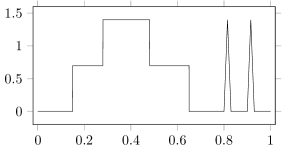
(a) LIDAR signal.

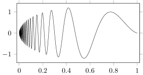
(b) Doppler signal.

(c) Cusp signal.

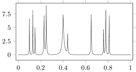
(d) Bumps signal.

Figure 1: Four signals that are common in signal processing and deconvolution.

(a) LIDAR signal.

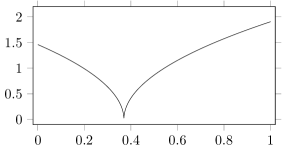
(b) Cusp signal.

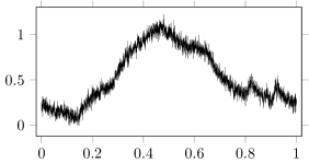
(c) Blurred signal with $\nu=0.7,\,\alpha=0.5$.

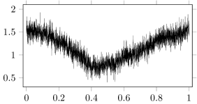
(d) Blurred signal with $\nu=0.7,\,\alpha=0.6$.

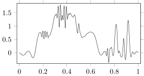
(e) Default WaveD reconstruction, $\widehat{j}_{1,1}=6$.

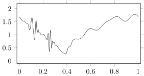
(f) Default WaveD reconstruction, $\widehat{j}_{1,1}=6$.

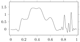
(g) LRD WaveD reconstruction, $\widehat{j}_{\alpha,1}=5$.

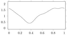
(h) LRD WaveD reconstruction, $\widehat{j}_{\alpha,1}=4$.

Figure 2: Comparison of the LRD WaveD method against the default WaveD method. In both cases, $n=4096=2^{12}$. The LRD method truncates the finest scale earlier as noted. For the LIDAR and cusp signals, SNR $\approx$ 20dB.

As will become evident in the later in the theoretical analysis. The case of LRD errors introduces some challenges to the estimation. For strong dependence there can be artificial trends in the noise which require modified thresholds in the wavelet estimator compared to the i.i.d. case. These effects are demonstrated clearly in Figure 2 for the cusp signal whereby the addition of a higher scale in the wavelet estimation deteriorates the performance of the standard WaveD method when there is a strong LRD error structure. Since the finest scale is too large, the i.i.d. method also includes the spurious trends which were artificially generated by the LRD error sequence.

1.1 Outline

A review of periodised Meyer wavelets and the Besov functional class are given in Section 2. In Section 3 the basic argument for the deconvolution technique is given along with the convergence rate results. In Section 4, the method is implemented in R and a numerical study is conducted to confirm the rate results and a compare with the current WaveD methodology. The mathematical proofs are given in Section 5.

2 Preliminary framework

2.1 Periodised Meyer wavelet basis

Let $\left(\phi,\psi\right)$ denote the Meyer wavelet scaling and detail basis functions defined on the real line $\mathbb{R}$; (see Meyer (1992) and Mallat (1999)). These are defined in the Fourier domain with,

$$\widetilde{\phi}(\omega)=\begin{cases}1,&\text{if }|\omega|\leq 1/3\\ \cos(\pi/2v(3|\omega|-1)),&\text{if }|\omega|\in(1/3,2/3]\\ 0,&\text{otherwise}.\end{cases}$$

and the mother wavelet function defined with,

$$\widetilde{\psi}(\omega)=\begin{cases}e^{-i\pi\omega}\sin(\frac{\pi}{2}v(3|\omega|-1)),&\text{if }|\omega|\in(1/3,2/3]\\ e^{-i\pi\omega}\cos(\frac{\pi}{2}v(3/2|\omega|-1)),&\text{if }|\omega|\in(2/3,4/3]\\ 0,&\text{otherwise}.\end{cases}$$ (3)

The auxiliary function $v$ is a piecewise polynomial that can be chosen to ensure that the Meyer wavelet has enough vanishing moments. For the bivariate index $(j,k)$, the dilated and translated mother and father wavelets at resolution level $j$ and time position $k$ are defined,

$$\phi_{j,k}(x)=2^{j/2}\phi(2^{j}x-k),\quad\psi_{j,k}(x)=2^{j/2}\psi(2^{j}x-k),\quad\text{for }j\geq 0.$$

For our purposes, we are interested with a multiresolution analysis for periodic functions on $\mathscr{L}_{2}([0,1])$. This is done by periodising the Meyer basis functions with,

$$\Phi_{j,k}(x)=\sum_{l\in\mathbb{Z}}\phi_{j,k}(x+l)\quad\text{and}\quad\Psi_{j,k}(x)=\sum_{l\in\mathbb{Z}}\psi_{j,k}(x+l).$$

Consequently, any $1-$periodic function $f\in\mathscr{L}_{2}([0,1])$ can be written with a wavlet expansion with,

$$f(x)=\sum_{k=j_{0}}^{2^{j_{0}}-1}\alpha_{j_{0},k}\Phi_{j_{0},k}(x)+\sum_{j=j_{0}}^{\infty}\sum_{k=0}^{2^{j}-1}\beta_{j,k}\Psi_{j,k}(x),$$

where $\alpha_{j_{0},k}=\langle{f},{\Phi_{j,k}}\rangle=\int_{0}^{1}f(t)\Phi_{j_{0},k}(t)\,dt$ and $\beta_{j,k}=\langle{f},{\Psi_{j,k}}\rangle=\int_{0}^{1}f(t)\Psi_{j,k}(t)\,dt$.

This particular expansion is used since the Meyer wavelet is bandlimited (see (3)) which allows the use of efficient algorithms with Raimondo and Stewart (2007) and for mathematical convenience in the later proofs.

2.2 Functional Class

We analyse the estimation procedure over a Besov space of periodic functions which have a nice characterisation using the coefficients of a wavelet expansion (granted that the wavelet is periodic and has enough smoothness and vanishing moments).

Definition 1

For $f\in\mathscr{L}_{\pi}([0,1])$ with $\pi\geq 1$ and $r\geq 1$,

$$f=\sum_{j,k}\beta_{j,k}\Psi_{j,k}(x)\in\mathcal{B}_{\pi,r}^{s}\Leftrightarrow\sum_{j\geq 0}2^{j(s+\tfrac{1}{2}-\tfrac{1}{\pi})r}\left(\sum_{k=0}^{2^{j}}\left|\beta_{j,k}\right|^{\pi}\right)^{\tfrac{r}{\pi}}<\infty.$$

The consideration of a Besov class allows a more precise analysis of the asymptotic convergence results of the signal $f$ since the Besov class includes other common functional classes as a special case. Loosely speaking, a function $f\in\mathcal{B}_{\pi,r}^{s}$ includes functions that are $s$ times differentiable with $f^{(s)}\in\mathscr{L}_{\pi}(0,1)$. The parameter $r$ is less important, it allows a more intricate variation of behaviour in the Besov class. The special cases when $\pi$ or $r=\infty$ involve replacing the $\ell_{\pi}$ and $\ell_{r}$ type norms in Definition 1 with the $\ell_{\infty}$ norm. For example, if $f\in\mathcal{B}^{s}_{\infty,\infty}\Rightarrow\sup_{j\geq 0}2^{j(s+1/2-1/\pi)}\sup_{(j,k)}|\beta_{j,k}|<\infty.$ The interested reader is referred to Donoho et al. (1995); Donoho and Johnstone (1998) and references therein for a more detailed discussion.

3 Function estimation method

We use the wavelet shrinkage paradigm for our estimation which has become a standard statistical procedure in nonparametric estimation. We use a hard thresholding approach where the wavelet estimator is defined,

$$\widehat{f}(x)=\sum_{k=0}^{2^{j_{0}}-1}\widehat{\alpha}_{j_{0},k}\mathbbm{1}_{\left\{|\widehat{\alpha}_{j_{0},k}|\geq\lambda_{j_{0}}\right\}}\Phi_{j_{0},k}(x)+\sum_{(j,k)\in\Lambda_{n}}^{2^{j}-1}\widehat{\beta}_{j,k}\Psi_{j,k}(x),$$ (4)

where $\widehat{\alpha}_{j_{0},k}$ and $\widehat{\beta}_{j_{0},k}$ are the estimated wavelet coefficients. The level $j_{0}$ corresponds to the coarse resolution level and the set of indices $\Lambda_{n}=\left\{(j,k):j_{0}\leq j\leq j_{1};k=0,1,\ldots,2^{j}-1\right\}$ indexes details of the function up to a fine resolution level $j_{1}$. The wavelet estimation procedure keeps only the coefficients in the expansion when $\left|\widehat{\beta}_{j,k}\right|\geq\lambda_{j}$, a scale dependent threshold. The parameters $\lambda_{j}$ and indices $\Lambda_{n}$ are chosen to control the noise embedded in the estimated wavelet coefficients in an optimal way in the sense of the rate results presented in the next section.

For the deconvolution problem it is natural to conduct analysis in the Fourier domain since the deconvolution operator becomes a multiplier in the Fourier domain. The deconvolution model, (1), has Fourier domain representation with,

$$\widetilde{Y}[n]\coloneqq\int_{\mathbb{R}}e^{-2\pi inx}\,dY(x)=\widetilde{K}[n]\widetilde{f}[n]+\varepsilon^{\alpha}\widetilde{Z}_{H}[n].$$

Then using the Parseval identity, one can obtain a representation of the wavelet coefficients.

$$\widehat{\beta}_{j,k} =\sum_{n\in\mathbb{Z}}\frac{\widetilde{Y}[n]}{\widetilde{K}[n]}\overline{\widetilde{\Psi_{j,k}}}[n]$$

$$=\sum_{n\in\mathbb{Z}}\widetilde{f}[n]\overline{\widetilde{\Psi_{j,k}}}[n]+\varepsilon^{\alpha}\sum_{n\in\mathbb{Z}}\frac{\widetilde{Z_{H}}[n]}{\widetilde{K}[n]}\overline{\widetilde{\Psi_{j,k}}}[n]$$

$$=\beta_{j,k}+\varepsilon^{\alpha}\sum_{n\in\mathbb{Z}}\frac{\widetilde{Z_{H}}[n]}{\widetilde{K}[n]}\overline{\widetilde{\Psi_{j,k}}}[n]$$ (5)

The Meyer wavelet is bandlimited (see (3)) meaning that the sums are finite. In particular, define the summation sets for the detail coefficients at scale level $j$ with,

$$\mathbb{D}_{j}\coloneqq\left\{z=\pm a:a\in\left\{\lceil 2^{j}/3\rceil,\lceil 2^{j}/3\rceil+1,\ldots,\lfloor 2^{j+2}/3\rfloor\right\}\right\},$$ (6)

which has cardinality $|\mathbb{D}_{j}|=2^{j+1}$. A similar procedure is conducted to estimate the scale coefficients $\alpha_{j_{0},k}$ by using the Fourier coefficients of the scale function $\Phi_{j_{0},k}$ instead of the detail function $\Psi_{j,k}$.

3.1 Maxiset Approach

The methodology used here is an amalgamation of the deconvolution work of Johnstone et al. (2004) and the LRD work of Kulik and Raimondo (2009b). The nonlinear wavelet estimator (4) can be analysed using the maxiset approach with the level dependent threshold $\lambda=\lambda_{j}$ and fine resolution level $j_{1}$ which depends on $\alpha$ and $\nu$.

Fine resolution level. The range of resolution levels (frequencies) where the estimator (4) is considered is,

$$\Lambda_{n}=\left\{(j,k):j_{0}\leq j\leq j_{1},0\leq k\leq 2^{j}\right\}.$$ (7)

The finest resolution level $j_{1}$ is set to be,

$$2^{j_{1}}=2^{j_{\alpha,1}}\coloneqq\left(\frac{n^{\alpha}}{\log n}\right)^{1/(\alpha+2\nu)},$$ (8)

Then consider the precise form of the level dependent thresholds in $\lambda=\lambda_{j}$. As in previous works, this level dependent threshold will have three input parameters, written,

$$\lambda_{j}=\xi\sigma_{j,\nu,\alpha}c_{n},$$ (9)

where the three values are given by,

• $\xi$ : a constant that depends on the tail of the noise distribution. Theoretically this should satisfy the bound $\xi>2\sqrt{\alpha(p\vee 2)}$.

• $\sigma_{j}$: the level-dependent scaling factor that is based on the convolution kernel and level of dependence,

  $$\sigma_{j}=\sigma_{j,\nu,\alpha}=\mathcal{O}(2^{-j(1-\alpha-2\nu)/2}).$$ (10)

• $c_{n}$ : a sample size dependent scaling factor,

  $$c_{n}=\sqrt{n^{-\alpha}\log n}.$$ (11)

The smoothing parameter is intentionally denoted $\xi$ to distinguish it clearly from the smoothing parameter, denoted $\eta$ used in the i.i.d. case in Johnstone et al. (2004) and its WaveD implementation in Raimondo and Stewart (2007).

Theorem 1

Consider model (1) with the wavelet estimator (4) with the coefficient estimates in (5) using the thresholds and resolution levels given by, (7), (8), (9), (10) and (11). Assume that $p>1$ and $f\in\mathcal{B}^{s}_{\pi,r}$ with $\pi\geq 1$, $s\geq 1/\pi$ where $r$ satisfies

$$0<r\leq\min\left\{\frac{(2\nu+\alpha)p}{2s+2\nu+\alpha},\frac{(2\nu+\alpha)p-2}{2s+2\nu-\frac{2}{\pi}\alpha}\right\}.$$

Then there exists a constant $C>0$ such that,

$$\mathbb{E}\left\lVert f-\widehat{f}\right\rVert_{p}^{p}\leq C\left(\frac{\log n}{n}\right)^{\rho},$$

where $\left\lVert\cdot\right\rVert_{p}$ is the standard $p$-norm and,

$$\frac{\alpha sp}{2s+2\nu+\alpha}, \quad\text{if }\quad s\geq(2\nu+\alpha)\left(\frac{p}{2\pi}-\frac{1}{2}\right);$$ (12)

$$\frac{\alpha p(s-\tfrac{1}{\pi}+\tfrac{1}{p})}{2s+2\nu+\alpha-\frac{2}{\pi}}, \quad\text{if }\quad\frac{1}{\pi}-\nu-\frac{\alpha}{2}<s<(2\nu+\alpha)\left(\frac{p}{2\pi}-\frac{1}{2}\right).$$ (13)

Remark 1

There is an ‘elbow effect’ or ‘phase transition’ in the rates of convergence switching from (12) to (13) which are usually referred to as the ‘dense’ and ‘sparse’ phases respectively. This is similar to the effect seen in Kulik and Raimondo (2009a) and Johnstone et al. (2004). The fBm errors has increased the size of the dense region in comparison to the standard Brownian motion when the boundary was at $s=(2\nu+1)(p/2\pi-1/2)$ (see Johnstone et al. (2004)). Also for the sparse region, the condition $p>2/(2\nu+\alpha)$ is needed to ensure that it is well defined. When $2\nu+\alpha\geq 2$, this is not a restriction since it is assumed that $p>1$.

Remark 2

The rate results are consistent with works on LRD and inverse problems in the literature in the sense that the rate of convergence deteriorates as $\alpha$ decreases (stronger dependence) or the DIP parameter $\nu$ increases (more ill-posed). In particular, our rate results agree with the results obtained in Johnstone et al. (2004) in the i.i.d. deconvolution setting with smooth convolution, $|\widetilde{K}(\omega)|\sim|\omega|^{-\nu}$, with the choice $\alpha=1$. Our rate results also agree with the results obtained in Kulik and Raimondo (2009a) with the direct regression model with LRD errors with the choice $\nu=0$. The results agree with minimax results the for the squared-error loss ($p=2$) by Wang (1997).

Remark 3

Our estimator is adaptive with respect to the smoothness parameter $s$ since the tuning paradigm does not depend on $s$. However it is not adaptive with respect to the LRD parameter $\alpha$ since the level dependent thresholds, (8), (10) and (11) depend on $\alpha$.

4 Numerical Study

A numerical study is now considered with the focus being the effect of the dependence structure. Ideally, it would be desirable to compare the LRD WaveD method introduced here with the minimax optimal WVD method considered by Wang (1997). However, to the authors knowledge, no freely available implementation of the WVD method exists.

One of the immediate challenges of implementing the LRD approach is that $\alpha$ is unknown in practice. The estimation of $\alpha$ is challenging problem in its own right that has been studied in the literature, see for example Veitch and Abry (1999) and more recently Park and Park (2009) in this regard. Having full data driven estimates of all the parameters is beyond the scope of this work and we will assume that $\alpha$ is known. For our purposes we wish to compare the performance of the regular WaveD approach which was designed for i.i.d. observations with the LRD extension suggested here.

The default WaveD method uses a stopping rule in the Fourier domain using the results of Cavalier and Raimondo (2007) to estimate the finest permissible scale level in the expansion. This concerns the case of model (1) with a standard Brownian motion ($\alpha=1$) where $2^{j_{1}}=2^{j_{1,1}}=(n/\log n)^{1/(1+2\nu)}$. For a fair comparison, the finest permissible scale level, $j_{\alpha,1}$, should be estimated in the same vein for our LRD extension. The Fourier stopping rule is extended to the LRD framework below.

Briefly reviewing the fine scale estimation method of Cavalier and Raimondo (2007), the scenario of an unknown convolution kernel $K$ is considered. To alleviate this they assume that it is possible to choose input signals $f$ in (1) to gain information about $K$. In particular, the Fourier basis is chosen $f=\left(e_{\ell}\right)_{\ell\in\mathbb{Z}}$ and passed into the deconvolution model. Doing so here, one would pass the Fourier basis into (1) and denote this new information with $dY_{e}(x)=K*e_{\ell}(x)+\varepsilon^{\alpha}dB_{H}(x)$. Due to the orthogonality of the Fourier basis, the Fourier domain representation of $Y_{e}$ is

$$\widetilde{Y}_{e}[\ell]=\widetilde{K}[\ell]+\varepsilon^{\alpha}W_{H}[\ell]$$

where $\widetilde{W}_{H}[\ell]$ is a complex Gaussian random variable identically distributed to $\widetilde{Z}_{H}[\ell]$ but independent of $\widetilde{Z}_{H}[\ell]$. We then estimate the fine scale level by,

$$\widehat{j}_{\alpha,1}=\lfloor\log_{2}M\rfloor-1$$ (14)

where the stopping time $M$ is determined in the Fourier domain with,

$$M=\min\left\{\ell,\ell>0:|\widetilde{Y}_{e}[\ell]|\leq\ell^{\alpha/2}\varepsilon^{\alpha}\log 1/\varepsilon^{2}\right\},$$

and $\lfloor x\rfloor$ is the largest integer small than $x$. The estimate $\widehat{j}_{\alpha,1}$ is close to $j_{\alpha,1}$ with high probability due to Lemma 1 in Section 5.

4.1 Implementation procedure

We are now in a position to be able to implement an estimation procedure for the LRD model (1) using a modification of WaveD method of Raimondo and Stewart (2007). This is conducted using the test functions shown in Figure 1. A discretely sampled deconvolution model is repeatedly simulated with these test signals and the WaveD and LRD modification estimates computed. The performance measure is the Mean-Square Error (MSE) which is calculated empirically over $M=1024$ repeated simulations.

1. Choose $f(t)$ to be a LIDAR, Doppler, Bumps or Cusp signal (see Figure 1) over the grid $t_{i}=i/n$ with $i=1,2,\ldots,n$ and $n=2^{12}=4096$. The LIDAR and Doppler signals were generated from by the code from the WaveD package and the Bumps and Cusp signal code was imported into R from the WaveLab package in MATLAB. The signals were standardised to agree with the signal levels in Cavalier and Raimondo (2007).

2. Simulate the LRD error process using the fracdiff package of R available from CRAN. Use the fracdiff.sim command to simulate a FARIMA sequence, the parameters kept at their defaults with the dependence controlled with $d=(1-\alpha)/2$ and the LRD error process was standardised to have unit variance.

3. Generate the convolution kernel, $K=k$, to be the Gamma density with scale parameter $0.25$ and shape parameter $0.7$ (The $DIP$ in this case is $\nu=0.7$).

4. Generate the data $y_{i}=k*f(t_{i})+\sigma 2^{-\alpha/2}e_{i}$ where $e_{i}$ is the FARIMA sequence. The size of $\sigma$ is governed by the blurred signal-to-noise ratio (SNR) where

   $$\text{SNR}=10\log_{10}\left(\left\lVert K*f\right\rVert^{2}/\sigma^{2}\right)$$

   The SNR is considered for three scenarios SNR = 10dB (high noise), 20dB (medium noise) or 30dB (low noise).

5. Compute the default WaveD estimator which assumes three vanishing moments and starts the wavelet expansion at scale level $j_{0}=3$. The level dependent thresholds are computed, $\lambda_{j}=\eta\tau_{j}c_{n}$ where $\eta=\sqrt{6}$, $c_{n}=\widehat{\sigma}\sqrt{\log n/n}$ and $\tau_{j}=(|\mathbb{D}_{j}|^{-1}\sum_{\mathbb{D}_{j}}|K[\ell]|^{-2})^{-1/2}$. The estimated noise level, $\widehat{\sigma}=MAD(y_{J,k})/0.6745$ where $MAD$ is the median absolute deviations and $y_{J,k}=\langle{y},{\Psi_{J,k}}\rangle$, the wavelet coefficients at the finest scale. The fine scale $j_{1}=j_{1,1}$ is estimated using the default WaveD method which is based on Cavalier and Raimondo (2007).

6. Compute the LRD WaveD estimator which uses the same hard thresholding wavelet expansion. However, now the fine scale level and level dependent thresholds are modified. The fine scale level, $j_{1}=j_{\alpha,1}$ is estimated using (14) and the level dependent thresholds are estimated using $\widehat{\lambda}_{j}=\xi\tau_{\alpha,j}c_{n}$ where $c_{n}=\widehat{\sigma}\sqrt{\log n/n^{\alpha}}$ and $\tau_{\alpha,j}$ calculated using (31) and (33). The smoothing parameter $\xi$ was tested for various different values. Similar to the i.i.d. case seen in Johnstone et al. (2004), the default bound given in the theory with $\xi\geq 2\sqrt{2\alpha}$ was much too conservative. Instead the performance was found to be much better with the choice $\xi=\sqrt{\alpha}$. The presented results here are for the choices $\xi=\sqrt{\alpha}$ and $\xi=\sqrt{2\alpha}$, the latter being more effective with low levels of $\alpha$. In fact, the simulations were also conducted for $\xi=\sqrt{4\alpha},\sqrt{6\alpha}$ and $\sqrt{8\alpha}$. These bigger smoothing parameters were only competitive for the cases when $\alpha\leq 0.3$ and are omitted from the tables for brevity.

7. Compute the empirical version of the MSE where,

   $$\widehat{MSE}(\widehat{f},f)=\widehat{\mathbb{E}}\left\lVert\widehat{f}-f\right\rVert^{2}_{2}=\frac{1}{M}\sum_{i=1}^{M}\left\lVert\widehat{f}_{i}-f\right\rVert_{2}^{2}.$$

$DIP=0.7$		$\alpha$
Signal	Method	1	0.8	0.6	0.4	0.2
Cusp	i.i.d.	0.0056 (3)	0.0089 (3)	0.0557 (4)	0.2525 (4)	0.6633 (4)
10dB	$\xi=\sqrt{\alpha}$	0.0056 (3)	0.0091 (3)	0.0238 (3)	0.0728 (3)	0.2235 (3)
	$\xi=\sqrt{2\alpha}$	0.0056 (3)	0.0091 (3)	0.0223 (3)	0.0606 (3)	0.1895 (3)
Cusp	i.i.d.	0.0035 (5)	0.0039 (5)	0.0148 (5)	0.0650 (5)	0.1683 (5)
20dB	$\xi=\sqrt{\alpha}$	0.0030 (5)	0.0037 (4)	0.0070 (4)	0.0099 (3)	0.0243 (3)
	$\xi=\sqrt{2\alpha}$	0.0039 (5)	0.0042 (4)	0.0054 (4)	0.0084 (3)	0.0206 (3)
Cusp	i.i.d.	0.0013 (6)	0.0014 (6)	0.0036 (6)	0.0148 (6)	0.0392 (6)
30dB	$\xi=\sqrt{\alpha}$	0.0011 (6)	0.0014 (5)	0.0025 (5)	0.0059 (5)	0.0069 (4)
	$\xi=\sqrt{2\alpha}$	0.0015 (6)	0.0016 (5)	0.0020 (5)	0.0034 (5)	0.0055 (4)
LIDAR	i.i.d.	0.0430 (4)	0.0418 (4)	0.0517 (4)	0.0972 (4)	0.4365 (5)
10dB	$\xi=\sqrt{\alpha}$	0.0363 (4)	0.0403 (4)	0.0512 (3)	0.0636 (3)	0.0993 (3)
	$\xi=\sqrt{2\alpha}$	0.0473 (4)	0.0488 (4)	0.0548 (3)	0.0633 (3)	0.0913 (3)
LIDAR	i.i.d.	0.0128 (5)	0.0133 (5)	0.0167 (5)	0.0483 (6)	0.1100 (6)
20dB	$\xi=\sqrt{\alpha}$	0.0103 (5)	0.0122 (5)	0.0248 (4)	0.0299 (4)	0.0393 (4)
	$\xi=\sqrt{2\alpha}$	0.0151 (5)	0.0164 (5)	0.0262 (4)	0.0305 (4)	0.0382 (4)
LIDAR	i.i.d.	0.0049 (6)	0.0049 (7)	0.0060 (7)	0.0111 (7)	0.0230 (7)
30dB	$\xi=\sqrt{\alpha}$	0.0041 (6)	0.0044 (6)	0.0057 (6)	0.0088 (6)	0.0103 (5)
	$\xi=\sqrt{2\alpha}$	0.0053 (6)	0.0054 (6)	0.0059 (6)	0.0073 (6)	0.0096 (5)

Table 1: MSE for the Bumps and Cusp signals with $n=4096$ and $M=1024$, the smoothing parameter for the LRD WaveD method is $\xi=\sqrt{\alpha}$, the i.i.d. method uses the default $\eta=\sqrt{6}$. The typical estimated fine scale levels are shown in parentheses for each case.

$DIP=0.7$		$\alpha$
Signal	Method	1	0.8	0.6	0.4	0.2
Bumps	i.i.d.	0.7657 (4)	0.7717 (4)	0.7904 (4)	0.8277 (4)	0.9475 (5)
10dB	$\xi=\sqrt{\alpha}$	0.7615 (4)	0.7705 (4)	0.9376 (3)	0.9511 (3)	0.9831 (3)
	$\xi=\sqrt{2\alpha}$	0.7687 (4)	0.7768 (4)	0.9380 (3)	0.9517 (3)	0.9818 (3)
Bumps	i.i.d.	0.5384 (5)	0.5405 (5)	0.2905 (6)	0.2702 (6)	0.3165 (6)
20dB	$\xi=\sqrt{\alpha}$	0.5374 (5)	0.5405 (5)	0.5469 (5)	0.7583 (4)	0.7661 (4)
	$\xi=\sqrt{2\alpha}$	0.5391 (5)	0.5417 (5)	0.5473 (5)	0.7583 (4)	0.7660 (4)
Bumps	i.i.d.	0.0793 (7)	0.0807 (7)	0.0838 (7)	0.0897 (7)	0.0988 (7)
30dB	$\xi=\sqrt{\alpha}$	0.0777 (7)	0.2074 (6)	0.2093 (6)	0.21246 (6)	0.3141 (6)
	$\xi=\sqrt{2\alpha}$	0.0811 (7)	0.2080 (6)	0.2094 (6)	0.2118 (6)	0.3133 (6)
Doppler	i.i.d.	0.0278 (5)	0.0293 (5)	0.0369 (5)	0.0631 (5)	0.1199 (5)
10dB	$\xi=\sqrt{\alpha}$	0.0263 (5)	0.0472 (4)	0.0570 (4)	0.0689 (4)	0.1203 (3)
	$\xi=\sqrt{2\alpha}$	0.0292 (5)	0.0481 (4)	0.0568 (4)	0.0666 (4)	0.1196 (3)
Doppler	i.i.d.	0.0103 (6)	0.0106 (6)	0.0122 (6)	0.0183 (6)	0.0455 (7)
20dB	$\xi=\sqrt{\alpha}$	0.0096 (6)	0.0104 (6)	0.0200 (5)	0.0257 (5)	0.0304 (5)
	$\xi=\sqrt{2\alpha}$	0.0107 (6)	0.0110 (6)	0.0197 (5)	0.0248 (5)	0.0284 (5)
Doppler	i.i.d.	0.0029 (7)	0.0030 (7)	0.0032 (7)	0.0043 (8)	0.0075 (8)
30dB	$\xi=\sqrt{\alpha}$	0.0027 (7)	0.0029 (7)	0.0036 (7)	0.0055 (7)	0.0094 (7)
	$\xi=\sqrt{2\alpha}$	0.0031 (7)	0.0031 (7)	0.0033 (7)	0.0039 (7)	0.0066 (7)

Table 2: MSE for the Doppler and LIDAR signals with $n=4096$ and $M=1024$, the smoothing parameter for the LRD WaveD method is $\xi=\sqrt{\alpha}$, the i.i.d. method uses the default $\eta=\sqrt{6}$. The typical estimated fine scale levels are shown in parentheses for each case.

4.2 Numerical results

The results of the procedure are outlined in Table 1 and Table 2. As stated earlier, the focus of the numerical study is the effect of the dependence structure so the DIP is fixed at $\nu=0.7$. The most obvious fact is that overall the convergence rate tends to deteriorate as the level of dependence increases. This is consistent with the theoretical results in Section 3.

The numerical results are not overall conclusive in favour of one method over the other for all noise levels. The main complication arises in the truncation of the wavelet expansion with the fine scale levels $\widehat{j}_{1}$ and $\widehat{j}_{\alpha,1}$. The typical fine scale levels (rounded to the nearest integer) are shown in Table 1 and Table 2 stated in parentheses for each case for each method. Due to the construction, $j_{\alpha,1}\leq j_{1,1}$ for all $\alpha\in(0,1]$ and this is reflected in their estimates shown in Table 1 and Table 2. As expected $\widehat{j}_{\alpha,1}$ decreases as $\alpha$ increases (stronger dependence) which is consistent with the theory. On the other hand, the naïve i.i.d. estimator increases as $\alpha$ decreases which can be either detrimental or beneficial to estimation as discussed below.

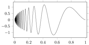
(a) Doppler signal.

(b) Bumps signal.

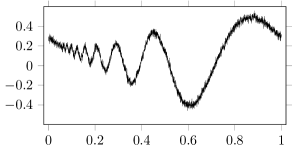
(c) Blurred signal with $\nu=0.7,\,\alpha=0.5$.

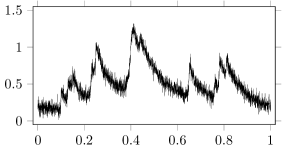
(d) Blurred signal with $\nu=0.7,\,\alpha=0.6$.

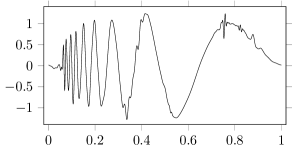
(e) Default WaveD reconstruction, $\widehat{j}_{1}=7$.

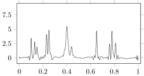
(f) Default WaveD reconstruction, $\widehat{j}_{1}=5$.

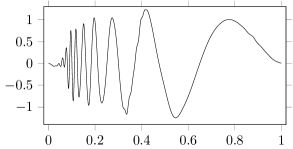
(g) LRD WaveD reconstruction, $\widehat{j}_{\alpha,1}=6$.

(h) LRD WaveD reconstruction, $\widehat{j}_{\alpha,1}=4$.

Figure 3: Comparison of the LRD WaveD method against the default WaveD method. In both cases, $n=4096=2^{12}$. The LRD method truncates the finest scale earlier as noted. For the Bumps and Doppler signals, SNR $\approx$ 20dB.

In some cases the earlier truncation in the LRD method is favourable such as the LIDAR and Cusp signals with a strong level of dependence which is shown in Figure 2. The addition of higher scales to the wavelet expansion in the i.i.d. method does contribute to capturing more of the cusp feature and the last two peaks of the LIDAR signal. However, it is paid at the price that higher scales include spurious effects from the LRD noise, resulting in a poor estimator. This is reflected in Table 1 where the MSE is smaller when $\widehat{j}_{\alpha,1}<\widehat{j}_{1}$ with the exception at the LIDAR signal at 20dB and $\alpha=0.6$ and the Cusp signal at 10dB and $\alpha=0.8$.

On the other hand, the earlier truncation of fine scale levels in the LRD method means that important features are not captured in the signal. This is seen in the Bumps and Doppler signals where the i.i.d. method tends to outperform the LRD method. In this situation the higher level scales in the expansion capture more features in the signal while not introducing the too much of the spurious LRD noise effects. A typical medium noise scenario demonstrating this is shown for the Bumps and Doppler signals in Figure 3. Referring to the Doppler deconvolution in Figure 3 one can see that the spurious trends generated by the LRD noise are included in the default WaveD reconstruction, however since $\widehat{j}_{1}>\widehat{j}_{\alpha,1}$, the higher frequences of the Doppler signal can be captured. The LRD method does not include the spurious trends but pays the price of losing the higher frequencies in the Doppler signal. A similar behaviour is present in the Bumps signal. This behaviour is reflected in the numerical study in Table 2 where the earlier truncation shows that the i.i.d. method outperforms the LRD method. However for the case of severely dependent noise at $\alpha=0.2$ for the Doppler signal, the i.i.d. method loses its advantage and the addition of higher scales does not outperform the LRD method.

Therefore the LRD estimation method presented here offers an easily implementable solution that is resistant to the effects of long memory. The method is attractive to the case where the underlying function $f$ does not have a lot of transient high frequency behaviours where the higher scales of the wavelet transform are crucial. In the case where high frequencies are crucial to the signal, the established i.i.d. WaveD method is perhaps more favourable since the signal features at higher scales are more important than the spurious noise.

5 Proofs

First the probabilistic result of the numerical estimation of the highest permissible scale level is given. Define the frequency levels,

$$M_{c} =\min\left\{\ell,\ell>0:|\widetilde{K}[\ell]|\leq\ell^{\alpha/2}\varepsilon^{\alpha}\left(\log 1/\varepsilon^{2}\right)^{4/3}\right\}$$ (15)

$$M_{d} =\min\left\{\ell,\ell>0:|\widetilde{K}[\ell]|\leq\ell^{\alpha/2}\varepsilon^{\alpha}\left(\log 1/\varepsilon^{2}\right)^{2/3}\right\}.$$ (16)

Lemma 1

Define the event, $\mathcal{B}=\cap_{\omega=1}^{M_{d}}\left\{|\varepsilon^{\alpha}\widetilde{Z}_{H}[\omega]|\leq|\widetilde{K}[\omega]|/2\right\}$. Then

$$P(\mathcal{B}^{c})\leq cM_{d}\exp\left\{-(\log 1/\varepsilon)^{1+\xi}\right\}\eqqcolon\Omega_{n}$$

for some constants $c,\xi>0.$ Further, define the event, $\mathcal{M}=\left\{M_{c}\leq M\leq M_{d}\right\}$ then $P(\mathcal{M}^{c})=\mathcal{O}(\Omega_{n})$ and $M_{c}\leq M_{d}\leq M_{1}$ where $M_{1}=\lfloor 2^{j_{1}}\rfloor$.

Proof of Lemma 1. First we prove the statement that, $P(\mathcal{B}^{c})\leq\Omega_{n}$. By definition of $M_{d}$ in (16) there exists a $c\in(0,1)$ such that for all $\omega=1,2,\ldots,M_{d}$; $|\widetilde{K}[\omega]|/2>\tfrac{c}{2}\ell^{\alpha/2}\varepsilon^{\alpha}\left(\log 1/\varepsilon\right)^{2/3}$. Thus,

$$P(\mathcal{B}^{c}) =P\left({\displaystyle\bigcup_{\omega=1}^{M_{d}}}\left\{|\varepsilon^{\alpha}\widetilde{Z}_{H}[\omega]|>\frac{|\widetilde{K}[\omega]|}{2}\right\}\right)$$

$$\leq\sum_{\omega=1}^{M_{d}}P\left(|\varepsilon^{\alpha}\widetilde{Z}_{H}[\omega]|>|\widetilde{K}[\omega]|/2\right)$$

$$\leq\sum_{\omega=1}^{M_{d}}P\left(|\widetilde{Z}_{H}[\omega]|>\frac{c}{2}\omega^{\alpha/2}\left(\log 1/\varepsilon^{2}\right)^{2/3}\right)$$

From (32), $\mathbb{V}\text{ar}\left(\widetilde{Z}_{H}[\omega]\right)\asymp|\omega|^{\alpha-1}$ and apply the tail inequality for Gaussian random variables, let $Z\sim\mathcal{N}(0,1)$, then there exists a constant $C>0$ such that,

$$P(\mathcal{B}^{c}) \leq\sum_{\omega=1}^{M_{d}}P\left(|Z|>c\omega^{1/2}\left(\log 1/\varepsilon^{2}\right)^{2/3}\right)$$

$$\leq CM_{d}\exp\left\{-\frac{1}{2}c^{2}\left(\log 1/\varepsilon\right)^{4/3}\right\}=\mathcal{O}(\Omega_{n}).$$ (17)

For $\mathcal{M}^{c}$ the event can be written $\mathcal{M}^{c}=\left\{M>M_{d}\right\}\cup\left\{M<M_{c}\right\}$ and start by considering the first scenario,

$$P(M>M_{d}) \leq P(\cap_{\omega=1}^{M_{d}}\left\{|\widetilde{Y}_{e}[\omega]|>\omega^{\alpha/2}\varepsilon^{\alpha}\log 1/\varepsilon^{2}\right\})$$

$$\leq P(|\widetilde{Y}_{e}[M_{d}]|>M_{d}^{\alpha/2}\varepsilon^{\alpha}\log 1/\varepsilon^{2})$$

$$\leq P(|\widetilde{Y}_{e}[M_{d}]|>M_{d}^{\alpha/2}\varepsilon^{\alpha}\log 1/\varepsilon^{2},\,\mathcal{B})+P(\mathcal{B}^{c})$$ (18)

Now under the event $\mathcal{B}$ with (2), $|\widetilde{Y}_{e}[M_{d}]|\leq\frac{3}{2}|\widetilde{K}[M_{d}]|\leq C|M_{d}|^{-\nu}$. Further, by definition of $M_{d}$ and (2)

$$M_{d}\asymp\left(\varepsilon^{\alpha}\left(\log 1/\varepsilon\right)^{2/3}\right)^{-2/(2\nu+\alpha)}$$ (19)

which means that as $n\to\infty$, $M_{d}^{-\nu-\alpha/2}=o(\varepsilon^{\alpha}(\log 1/\varepsilon^{2}))$. Hence, from (18) with (19) and (17), there is an $N\in\mathbb{Z}^{+}$ such that for all $n\geq N$,

$$P(M>M_{d})\leq P(M_{d}^{-\nu-\alpha/2}>\varepsilon^{\alpha}\log 1/\varepsilon^{2})+P(\mathcal{B}^{c})=P(\mathcal{B}^{c})=\mathcal{O}(\Omega_{n}).$$ (20)

On the other hand,

$$P(M<M_{c}) \leq P\left(\cup_{\omega=1}^{M_{c}-1}\left\{|\widetilde{Y}_{e}[\omega]|\leq\omega^{\alpha/2}\varepsilon^{\alpha}\log 1/\varepsilon^{2}\right\}\right)$$

$$\leq\sum_{\omega=1}^{M_{c}-1}P\left(|\widetilde{Y}_{e}[\omega]|\leq\omega^{\alpha/2}\varepsilon^{\alpha}\log 1/\varepsilon^{2}\right).$$

Under the event $\mathcal{B}$, $|\widetilde{Y}_{e}[\omega]|\geq|\widetilde{K}[\omega]|/2\geq cM_{c}^{-\nu}$ for all $\omega=1,2,\ldots,M_{c}-1.$ Similar to (19), by (15) and (2),

$$M_{c}\asymp\left(\varepsilon^{\alpha}\left(\log 1/\varepsilon^{2}\right)^{4/3}\right)^{-2/(2\nu+\alpha)}$$ (21)

and consequently, as $n\to\infty$, $\varepsilon^{\alpha}(\log 1/\varepsilon^{2})=o(M_{c}^{-\nu-\alpha/2})$. Hence from (17),

$$P(M<M_{c})\leq P(\mathcal{B}^{c})=\mathcal{O}(\Omega_{n}).$$ (22)

Therefore, (20) with (22) yields the first result of the Lemma. The second result of the Lemma follows from (19) and (21).

5.1 Maxiset Theorem

As in similar previous works in Kulik and Raimondo (2009a); Johnstone et al. (2004) the proof of the main result imitates the same maxiset approach. Roughly speaking, this approach finds the ‘maxiset’ class of functions for a general hard thresholding wavelet estimator. This Maxiset theorem is stated here for easy reference. First, introduce the notation: $\mu$ will denote the measure such that for $j\in\mathbb{N}$, $k\in\mathbb{N}$,

$$\mu\left\{(j,k)\right\} =\left\lVert\sigma_{j,\nu,\alpha}\Psi_{j,k}\right\rVert_{p}^{p}=\sigma_{j,\nu,\alpha}^{p}2^{j(\tfrac{p}{2}-1)}\left\lVert\Psi\right\rVert_{p}^{p},$$

$$l_{q,\infty}(m) =\left\{f,\sup_{\lambda>0}\lambda^{q}\mu\left\{(j,k):\left|\beta_{j,k}\right|>\sigma_{j,\nu,\alpha}\lambda\right\}<\infty\right\}.$$

Theorem 2 (Maxiset)

Let $p>0$, $0<q<p$ and $\left\{\Psi_{j,k},j\geq-1,k=0,1,\ldots,2^{j-1}\right\}$ be a periodised wavelet basis of $\mathscr{L}_{2}([0,1])$ and $\sigma_{j}$ is a positive sequence such that the heteroscedastic basis $\sigma_{j}\Psi_{j,k}$ satisfies the Temlyakov property. Suppose that the index set $\Lambda_{n}$ is a set of pairs ($j,k$) and $c_{n}$ is a deterministic sequence tending to zero with,

$$\sup_{n}\mu(\Lambda_{n})c_{n}^{p}<\infty.$$ (23)

If for any $n$ and any pair $(j,k)\in\Lambda_{n}$ we have,

$$\mathbb{E}|\widehat{\beta}_{j,k}-\beta_{j,k}|^{2p}\leq C(\sigma_{j}c_{n})^{2p};\qquad P(|\widehat{\beta}_{j,k}-\beta_{j,k}|\geq\xi\sigma_{j}c_{n}/2)\leq C(c_{n}^{2p}\wedge c_{n}^{4})$$ (24)

for some positive constants $\xi$ amd $C$ then the wavelet estimator,

$$\widehat{f}_{n}(x)=\sum_{(j,k)\in\Lambda_{n}}\widehat{\beta}_{j,k}\Psi_{j,k}(x)\mathbbm{1}_{\left\{|\widehat{\beta}_{j,k}|\geq\xi\sigma_{j}c_{n}\right\}}$$

satisfies the following for all positive integers $n$,

$$\mathbb{E}\left\lVert\widehat{f}_{n}-f\right\rVert_{p}^{p}\leq Cc_{n}^{p-q}.$$

if and only if,

$$f\in l_{q,\infty}(\mu)\quad\text{and}\quad\sup_{n\geq 1}\left(c_{n}^{q-p}\left\lVert f-\sum_{j,k\in\Lambda_{n}}\beta_{j,k}\Psi_{j,k}\right\rVert_{p}^{p}\right)<\infty.$$ (25)

The proof of the rate result in Theorem 1 will use the Maxiset Theorem by verifying the regularity conditions, (23), (24) and (25), then choosing $q$ for the dense and sparse regions respectively with,

$$q =q_{d}\coloneqq\frac{p(2\nu+\alpha)}{2s+2\nu+\alpha} \quad\text{when}\quad s\geq(\nu+\alpha/2)(p/\pi-1)$$ (26)

$$q =q_{s}\coloneqq\frac{(2\nu+\alpha)p-2}{2s+2\nu+\alpha-\frac{2}{\pi}} \quad\text{when }1/\pi-\alpha/2-\nu\leq s<(\nu+\alpha/2)(p/\pi-1)$$ (27)

5.2 Stochastic analysis of the estimated wavelet coefficients

By definition, it is clear that the estimated wavelet coefficients have no bias. Consider now the covariance structure of the $\widetilde{Z_{H}}$ process,

$$\mathbb{C}\text{ov}\left(\widetilde{Z_{H}}[\omega],\widetilde{Z_{H}}[\ell]\right)=\mathbb{E}\widetilde{Z_{H}}[\omega]\overline{\widetilde{Z_{H}}}[\ell]=\mathbb{E}\int_{\mathbb{R}}e^{-2\pi i\omega x}\,dB_{H}(x)\,\int_{\mathbb{R}}e^{2\pi i\ell y}\,dB_{H}(y).$$

To evaluate this, appeal to Theorem 2 of Wang (1996) which uses a representation of the fractional Gaussian noise process via a Wavelet-Vaguelette Decomposition (WVD)

$$dB_{H}(x)=\sum_{j,k}\xi_{j,k}u_{j,k}(x)\,dx,$$

where $\xi_{j,k}$ is a white noise process and $u_{j,k}$ is a set of vaguelette basis functions defined with,

$$u_{j,k}(x)\coloneqq(-\Delta)^{1/4-H/2}\varphi_{j,k}(x),$$

where $\Delta=\frac{d^{2}}{dx^{2}}$ is an elliptic operator and $\varphi_{j,k}\,{:}\,\mathbb{R}\!\longrightarrow\!\mathbb{R}$ is a set of orthogonal wavelet functions. Using this representation of fractional Gaussian noise we can write,

$$\mathbb{C}\text{ov}\left(\widetilde{Z_{H}}[\omega],\widetilde{Z_{H}}[\ell]\right) =\sum_{j,k}\sum_{j^{\prime},k^{\prime}}\mathbb{E}\xi_{j,k}\xi_{j^{\prime},k^{\prime}}\int_{\mathbb{R}}e^{-2\pi i\omega x}u_{j,k}(x)\,dx\,\int_{\mathbb{R}}e^{2\pi i\ell y}u_{j^{\prime},k^{\prime}}(y)\,dy.$$

$$=\sum_{j,k}\widetilde{u_{j,k}}[\omega]\overline{\widetilde{u_{j,k}}[\ell]}.$$ (28)

The operator $(-\Delta)^{-(H-1/2)/2}$ for $H\in(1/2,1)$ is known from the theory of singular integrals as the Reisz Potential (see for example Stein, 1970, Chapter V) and has the representation,

$$(-\Delta)^{-\tfrac{H-1/2}{2}}f(x)=\frac{\Gamma\left(\tfrac{3}{4}-\tfrac{H}{2}\right)}{\sqrt{\pi}2^{H-\tfrac{1}{2}}\Gamma\left(\tfrac{H}{2}-\tfrac{1}{4}\right)}\int_{\mathbb{R}}f(z)|z-x|^{H-3/2}\,dz.$$ (29)

For our purposes its behaviour in the Fourier domain has been evaluated by Samko, Kilbas, and Marichev (1993). Indeed, apply Theorem 12.2 of Samko et al. (1993) with (29) then for any $f\in\mathscr{L}_{1}(\mathbb{R})$,

$$\mathcal{F}(-\Delta)^{1/4-H/2}f(\omega) =\widetilde{f}(\omega)|\omega|^{1/2-H}.$$ (30)

From (28) and (30), it would be desirable to use a wavelet function $\varphi\in\mathscr{L}_{1}(\mathbb{R})$ that has a simple behaviour in the Fourier domain. Naturally, a suitable choice is the Meyer wavelet, $\varphi=\psi$, since it is bandlimited (see Section 2.1) and makes the calculations easier. Therefore we have,

$$\mathbb{C}\text{ov}\left(\widetilde{Z_{H}}[\omega],\widetilde{Z_{H}}[\ell]\right)=|\omega\ell|^{1/2-H}\sum_{j,k}\widetilde{\psi_{j,k}}(\omega)\overline{\widetilde{\psi_{j,k}}(\ell)}.$$ (31)

Consider an arbitrary $\omega\in\mathbb{Z}$ and consider the possible values of $j$ such that $\omega\in\mathbb{D}_{j}$. The summation sets will have a non empty intersection, $\mathbb{D}_{j}\cap\mathbb{D}_{j^{\prime}}\neq\emptyset$, if and only if $j^{\prime}\in\left\{j-1,j,j+1\right\}$. Therefore the summands in (31) will be nonzero for, at most, three different values of $j$. The Meyer wavelet also is bounded with, $|\widetilde{\psi}|\leq 1$. Therefore we can crudely bound the magnitude of the covariance with,

$$\left|\mathbb{C}\text{ov}\left(\widetilde{Z_{H}}[\omega],\widetilde{Z_{H}}[\ell]\right)\right| =|\omega\ell|^{1/2-H}\left|\sum_{j\in\mathbb{Z}}\sum_{k=0}^{2^{j}-1}2^{-j}e^{2^{1-j}\pi i(\ell-\omega)k}\widetilde{\psi}(\omega 2^{-j})\overline{\widetilde{\psi}(\ell 2^{-j})}\right|$$

$$\leq 3|\omega\ell|^{1/2-H}.$$ (32)

Thus we are in a position to bound the variance of the estimated wavelet coefficients,

$$\mathbb{V}\text{ar}\left(\widehat{\beta}_{j,k}\right) =\varepsilon^{2\alpha}\mathbb{V}\text{ar}\left(\sum_{\ell\in\mathbb{D}_{j}}\frac{\widetilde{Z_{H}}[\ell]}{\widetilde{K}[\ell]}\overline{\widetilde{\Psi_{j,k}}}[\ell]\right)$$

$$=\varepsilon^{2\alpha}\sum_{\omega\in\mathbb{D}_{j}}\sum_{\ell\in\mathbb{D}_{j}}\frac{\overline{\widetilde{\Psi_{j,k}}}[\ell]\widetilde{\Psi_{j,k}}[\omega]}{\widetilde{K}[\ell]\overline{\widetilde{K}}[\omega]}\mathbb{C}\text{ov}\left(\widetilde{Z_{H}}[\omega],\widetilde{Z_{H}}[\ell]\right)\eqqcolon\varepsilon^{2\alpha}\tau_{\alpha,j,k}^{2}.$$ (33)

To gain insight to the overall asymptotic structure, the variance of the coefficients needs to be bounded. Use (32) and that the cardinality of $\mathbb{D}_{j}$, $|\mathbb{D}_{j}|=2^{j+1}$,

$$\tau^{2}_{\alpha,j} \leq 3\sum_{\omega\in\mathbb{D}_{j}}\left|\frac{\widetilde{\Psi_{j,k}}[\omega]}{\overline{\widetilde{K}}[\omega]}\right||\omega|^{1/2-H}\sum_{\ell\in\mathbb{D}_{j}}\left|\frac{\overline{\widetilde{\Psi_{j,k}}}[\ell]}{\widetilde{K}[\ell]}\right||\ell|^{1/2-H}$$

$$=3\left(\sum_{\omega\in\mathbb{D}_{j}}\left|\frac{\widetilde{\Psi_{j,k}}[\omega]}{\overline{\widetilde{K}}[\omega]}|\omega|^{1/2-H}\right|\right)^{2}$$

$$\leq 3\left|\mathbb{D}_{j}\right|2^{-j}\sum_{\omega\in\mathbb{D}_{j}}\left|\frac{\widetilde{\Psi}[\omega 2^{-j}]}{\widetilde{K}[\omega]}\right|^{2}|\omega|^{1-2H}$$

$$\leq 6\sum_{\omega\in\mathbb{D}_{j}}\left|\frac{\widetilde{\Psi}[\omega 2^{-j}]}{\widetilde{K}[\omega]}\right|^{2}|\omega|^{1-2H}$$

$$\leq 6\sup_{x\in\mathbb{D}_{j}}|x|^{1-2H}\sup_{y\in\mathbb{D}_{j}}|\widetilde{K}[y]|^{-2}\int_{\mathbb{R}}|\widetilde{\Psi}(z)|^{2}\,dz$$

$$\leq C2^{-j(1-\alpha-2\nu)}\left\lVert\Psi\right\rVert_{2}^{2},$$

where the last two lines follow by Parseval and Plancherels identities and condition (2). Thus, the asymptotic behaviour of the variance of the wavelet coefficients at scale $j$ are bounded with,

$$\mathbb{V}\text{ar}\left(\widehat{\beta}_{j,k}\right)=\varepsilon^{2\alpha}\tau_{\alpha,j}^{2}\leq C\varepsilon^{2\alpha}2^{-j(1-\alpha-2\nu)}\leq C\sigma_{j,\nu,\alpha}^{2}c_{n}^{2},$$

where $\sigma_{j,\nu,\alpha}$ and $c_{n}$ are defined in (10) and (11). Since $\widehat{\beta}_{j,k}$ is Gaussian, then from the variance bound it follows that,

$$\mathbb{E}\left|\widehat{\beta}_{j,k}-\beta_{j,k}\right|^{2p}\leq C_{p}(\sigma_{j,\nu,\alpha}c_{n})^{2p}.$$

Let $\xi\geq\sqrt{4\alpha(p\vee 2)}$ and $Z\sim\mathcal{N}(0,1)$, then from the tail inequality for Gaussian random variables.

$$P\left(\left|\widehat{\beta}_{j,k}-\beta_{j,k}\right|\geq\frac{\xi\tau_{j,\nu,\alpha}c_{n}}{2}\right) =2P\left(Z\geq\frac{\xi\sqrt{\log n}}{2}\right)$$

$$\leq\frac{2\sqrt{2}}{\xi\sqrt{\pi\,\log n}}\exp\left\{-\frac{\xi^{2}\log n}{4}\right\}$$

$$\leq C_{\xi}n^{-\tfrac{\xi^{2}}{4}}\leq C(c_{n}^{2p}\wedge c_{n}^{4}).$$

This verifies the wavelet coefficient conditions in (24).

5.3 Temlyakov Property and resolution tuning

Recall $\Lambda_{n}=\left\{(j,k):-1\leq j\leq j_{\alpha,1};k=0,1,\ldots,2^{j}-1\right\}$. Consider the set of scales $\Lambda_{n}^{1}=\left\{j\in\mathbb{Z}:-1\leq j\leq j_{\alpha,1},j_{\alpha,1}\in\mathbb{Z}^{+}\right\}$. Then from Johnstone et al. (2004, Appendices A.1 & B.2), the heteroskedastic basis $\left\{\sigma_{j},\Psi_{j,k}(\cdot)\right\}$ satisfies the Temlyakov property as soon as,

$$\sum_{j\in\Lambda_{n}^{1}}2^{j}\sigma_{j}^{2}\leq C\sup_{j\in\Lambda_{n}^{1}}\left(2^{j}\sigma_{j}^{2}\right)\qquad\text{and}\qquad\sum_{j\in\Lambda_{n}^{1}}2^{jp/2}\sigma_{j}^{2}\leq C\sup_{j\in\Lambda_{n}^{1}}\left(2^{jp/2}\sigma_{j}^{p}\right).$$

This property is satisfied in our framework with $\sigma_{j}=\sigma_{j,\nu,\alpha}\leq C2^{-j/2(1-\alpha-2\nu)}$. Now verify the resolution tuning condition (23).

$$\mu(\Lambda_{n}) =\sum_{j\leq j_{\alpha,1}}2^{j}\sigma_{j,\nu,\alpha}^{p}2^{j(p/2-1)}\left\lVert\Psi\right\rVert_{p}^{p}<C2^{j_{\alpha,1}p(\alpha+2\nu)/2}.$$

Using the choice, $2^{j_{\alpha,1}}\asymp\left(n^{\alpha}/\log n\right)^{1/(\alpha+2\nu)}$ yields $\mu(\Lambda_{n})c_{n}^{p}=\mathcal{O}(1)$. Consequently, (23) is verified.

5.4 Besov Embedding

One needs to find a Besov scale such that $\mathcal{B}_{\pi,r}^{\delta}\subseteq l_{q,\infty}$ and that the maxiset condition (25) holds. As shown in Johnstone et al. (2004), the problem can be simplified by considering the the set of functions $l_{q}(\mu)\subset l_{q,\infty}(\mu)$ where,

$$l_{q}(\mu)\coloneqq\left\{f\in\mathscr{L}_{p}:\sum_{j,k\in A_{j}}\frac{\left|\beta_{j,k}\right|^{q}}{\sigma_{j}^{q}}\left\lVert\sigma_{j}\Psi_{j,k}\right\rVert_{p}^{p}<\infty\right\},$$

where $A_{j}$ is a set of cardinality proportional to $2^{j}$. Since $\left\lVert\sigma_{j}\Psi_{j,k}\right\rVert_{p}^{p}=\sigma_{j}^{p}2^{j(\tfrac{p}{2}-1)}$, then $f\in l_{q}(\mu)$ if

$$\sum_{j\geq 0}2^{\tfrac{j}{2}\left(p-2-(p-q)(1-\alpha-2\nu)\right)}\sum_{k=0}^{2^{j}-1}|\beta_{j,k}|^{q}=\sum_{j\geq 0}2^{jq\left((\nu+\tfrac{\alpha}{2})(\tfrac{p}{q}-1)+\tfrac{1}{2}-\tfrac{1}{q}\right)}\sum_{k=0}^{2^{j}-1}|\beta_{j,k}|^{q}<\infty.$$

This condition is true for $f\in\mathcal{B}_{q,q}^{\delta}$ with the choice $\delta=(\nu+\tfrac{\alpha}{2})(\tfrac{p}{q}-1).$ Then depending on whether we are in the dense or sparse case the levels $s,\pi$ and $r$ are determined such that $\mathcal{B}^{s}_{\pi,r}\subseteq\mathcal{B}_{q,q}^{\delta}$. There exists two Besov embeddings given by,

$$\mathcal{B}^{s}_{\pi,r} \subseteq\mathcal{B}^{\gamma}_{\rho,r}\qquad\text{when}\quad 0<\rho\leq\pi\text{ and }s\geq\gamma;$$ (34)

$$\mathcal{B}^{s}_{\pi,r} \subseteq\mathcal{B}^{\gamma}_{\rho,r}\qquad\text{when}\quad\pi<\rho\text{ and }s-1/\pi=\gamma-1/\rho.$$ (35)

The dense phase. Choose the level of $q=q_{d}$ where,

$$q_{d}\coloneqq\frac{p(2\nu+\alpha)}{2s+2\nu+\alpha}\qquad\text{when}\quad s\geq(\nu+\alpha/2)(p/\pi-1).$$

Then find the levels $s,\pi$ and $r$ such that $\mathcal{B}^{s}_{\pi,r}\subseteq\mathcal{B}_{q,q}^{\delta}$ where $s\geq(\nu+\alpha/2)(p/\pi-1)$.

By definition, one has, $s\geq\left(\alpha/2+\nu\right)\left(p/\pi-1\right)$. Eliminate $p$ by substituting $p=(2s+2\nu+\alpha)q_{d}/(2\nu+\alpha)$ yields, $\pi\geq q_{d}$. So we need to prove $s\geq\delta=\left(2\nu+\alpha\right)\left(p/2q_{d}-1/2\right)$ to be able to use (34). However, by definition of $q_{d}$ we have, $\delta=\left(\nu+\alpha/2\right)\left(p/q_{d}-1\right)=s>0$ by assumption.

The sparse phase. Choose the level of $q=q_{s}$ where,

$$q_{s}\coloneqq\frac{(2\nu+\alpha)p-2}{2s+2\nu+\alpha-\frac{2}{\pi}}\qquad\text{when}\quad 1/\pi-\alpha/2-\nu<s<(\nu+\alpha/2)(p/\pi-1).$$

To ensure the inequalities in the above equation are valid, it requires that $p>2/(2\nu+\alpha)$. Then $\delta=\left(2\nu+\alpha\right)\left(p/2q_{s}-1/2\right)$ and we have,

$$\delta =\left(2\nu+\alpha\right)\left(p/2q_{s}-1/2\right)$$

$$=\frac{(2\nu+\alpha)(sp-p/\pi+1)}{(2\nu+\alpha)p-2}.$$

Consider the scenario when $\pi\geq q_{s}$ and use embedding (34). This requires that $s\geq\delta=(2\nu+\alpha)(sp-p/\pi+1)/((2\nu+\alpha)p-2)$, or equivalently, $s\leq(\nu+\alpha/2)(p/\pi-1).$ It is also needed that $\delta>0$, which implies that either $(i)$ $p>2/(2\nu+\alpha)$ and $s>1/\pi-1/p$; or $(ii)$ $p<2/(2\nu+\alpha)$ and $s<1/\pi-1/p$. The $(ii)$ scenario is impossible since it is assumed that $p\geq 1$ and $s\geq 1/\pi$ which contradicts $s<1/\pi-1/p$. The condition $p>2/(2\nu+\alpha)$ is verified since by assumption in the sparse phase, $\nu\geq 1-\alpha/2$ and $p>1$. Then $(i)$ implies that, $s\geq 1/\pi-\nu-\alpha/2$.

Consider now the scenario when $\pi<q_{s}$ by definining,

$$s^{\prime}=s-1/\pi+1/q.$$ (36)

Then use the embedding (35). Indeed, if we solve (36) with $s^{\prime}=\delta$, then $q=q_{s}$ and the embedding of (35) applies.

To apply Theorem 2, (25) needs to be verified. Therefore we need to find a $\delta>0$ such that for any $f\in\mathcal{B}_{p,r,}^{\delta}$, (25) is satisfied.

$$c_{n}^{q-p}\left\lVert f-\sum_{j,k}\beta_{j,k}\Psi_{j,k}\right\rVert_{p}^{p}=c_{n}^{q-p}2^{-j_{\alpha,1}\delta p}\left\lVert f\right\rVert_{\mathcal{B}_{p,r}^{\delta}}=c_{n}^{q-p+2\delta p/(2\nu+\alpha)}\left\lVert f\right\rVert_{\mathcal{B}_{p,r}^{\delta}}.$$

The above is bounded uniformly in $n$ if we choose $\delta=1/2(2\nu+\alpha)(1-q/p)$. Now we need to find $s,\pi$ such that $\mathcal{B}_{\pi,r}^{s}\subseteq\mathcal{B}_{p,r}^{\delta}$.

Consider the first case $\pi\geq p$. This case cannot occur in the sparse phase due to (13) and the assumption that $s$ is positive. In the dense phase, use embedding (34) with $\gamma=\delta$ and $q=q_{d}$. Therefore, (34) holds if $s\geq 1/2(2\nu+\alpha)(1-q_{d}/p)$. This implies,

$$s \geq 1/2(2\nu+\alpha)(1-q_{d}/p)$$

$$=\frac{(2\nu+\alpha)s}{2s+2\nu+\alpha},$$

which always holds under the assumption that $s>0$.

Now consider the dense case when $\pi<p$. In this scenario use embedding (35) by defining $s-1/\pi=\gamma-1/p$ which ensures $\mathcal{B}_{\pi,r}^{s}\subseteq\mathcal{B}_{p,r}^{\gamma}$. Then complete the embedding using (34) (namely, $\mathcal{B}_{p,r}^{\gamma}\subseteq\mathcal{B}_{p,r}^{\delta}$) which requires $\gamma\geq\delta$ with $q=q_{d}$ or equivalently after rearrangement, $2s\gamma+(2\nu+\alpha)(1/p-1/\pi)\geq 0.$ The left hand side is greater than $(s-1/\pi)(p/\pi-1)(2\nu+\alpha)\geq 0$ when $s\geq(\nu+\alpha/2)(p/\pi-1)$ (which is true in the dense phase).

The last case to consider is the sparse case when $\pi<p$. Again introduce a new Besov scale $\gamma$ defined with, $s-1/\pi=\gamma-1/p$ and apply a similar argument to above which requires that, $\gamma\geq\delta$ with $q=q_{s}$. This is satisfied if $s>1/\pi$, which always holds.

5.5 Proof of Theorem 1

The proof of the theorem is an application of Theorem 2 with the choice of $\sigma_{j}=\sigma_{j,\nu,\alpha}$ and $c_{n}$ and $\xi$ defined in Section 3.1 and the arguments in Section 5.2, Section 5.3 and Section 5.4. The dense regime rate result of (12) is derived with the choice of $q=q_{d}$ in (26) and the Besov embedding argument in Section 5.4. Similarly, the sparse rate regime in (13) is derived with the Besov embedding result in Section 5.4 with the choice of $q=q_{s}$ in (27).

References

• Abramovich and Silverman (1998) Abramovich, F., Silverman, B.Β W., 1998. Wavelet decomposition approaches to statistical inverse problems. Biometrika 85Β (1), 115–129.
URL http://dx.doi.org/10.1093/biomet/85.1.115
• Beran (1992) Beran, J., 1992. Statistical Methods for Data with Long-Range Dependence. Statistical Science 7Β (4), 404–416.
URL http://dx.doi.org/10.1214/ss/1177011127
• Beran (1994) Beran, J., 1994. Statistics for long-memory processes. Vol.Β 61 of Monographs on Statistics and Applied Probability. Chapman and Hall, New York.
• Cavalier and Raimondo (2007) Cavalier, L., Raimondo, M., 2007. Wavelet deconvolution with noisy eigenvalues. IEEE Trans. Signal Process. 55Β (6, part 1), 2414–2424.
URL http://dx.doi.org/10.1109/TSP.2007.893754
• Chesneau (2012) Chesneau, C., 2012. On the adaptive wavelet deconvolution of a density for strong mixing sequences. J. Korean Statist. Soc.
URL http://dx.doi.org/10.1016/j.jkss.2012.01.005
• Donoho etΒ al. (1995) Donoho, D., Johnstone, I., Kerkyacharian, G., Picard, D., 1995. Wavelet Shrinkage - Asymptopia. Journal of the Royal Statistical Society Series B-Methodological 57Β (2), 301–337.
• Donoho (1995) Donoho, D.Β L., 1995. Nonlinear solution of linear inverse problems by wavelet-vaguelette decomposition. Appl. Comput. Harmon. Anal. 2Β (2), 101–126.
URL http://dx.doi.org/10.1006/acha.1995.1008
• Donoho and Johnstone (1998) Donoho, D.Β L., Johnstone, I.Β M., 1998. Minimax estimation via wavelet shrinkage. Ann. Statist. 26Β (3), 879–921.
URL http://dx.doi.org/10.1214/aos/1024691081
• Donoho and Raimondo (2004) Donoho, D.Β L., Raimondo, M.Β E., 2004. Translation invariant deconvolution in a periodic setting. Int. J. Wavelets Multiresolut. Inf. Process. 2Β (4), 415–431.
• Doukhan etΒ al. (2003) Doukhan, P., Oppenheim, G., Taqqu, M.Β S. (Eds.), 2003. Theory and applications of long-range dependence. BirkhΓ€user Boston Inc., Boston, MA.
• Fan and Koo (2002) Fan, J., Koo, J.-Y., 2002. Wavelet deconvolution. IEEE Trans. Inform. Theory 48Β (3), 734–747.
URL http://dx.doi.org/10.1109/18.986021
• Johnstone etΒ al. (2004) Johnstone, I.Β M., Kerkyacharian, G., Picard, D., Raimondo, M., 2004. Wavelet deconvolution in a periodic setting. J. R. Stat. Soc. Ser. B Stat. Methodol. 66Β (3), 547–573.
URL http://dx.doi.org/10.1111/j.1467-9868.2004.02056.x
• Johnstone and Raimondo (2004) Johnstone, I.Β M., Raimondo, M., 2004. Periodic boxcar deconvolution and Diophantine approximation. Ann. Statist. 32Β (5), 1781–1804.
• Kalifa and Mallat (2003) Kalifa, J., Mallat, S., 2003. Thresholding estimators for linear inverse problems and deconvolutions. Ann. Statist. 31Β (1), 58–109.
URL http://dx.doi.org/10.1214/aos/1046294458
• Kulik (2008) Kulik, R., 2008. Nonparametric deconvolution problem for dependent sequences. Electron. J. Stat. 2, 722–740.
URL http://dx.doi.org/10.1214/07-EJS154
• Kulik and Raimondo (2009a) Kulik, R., Raimondo, M., 2009a. L${}^{p}-$wavelet regression with correlated errors and inverse problems. Statist. Sinica 19Β (4), 1479–1489.
• Kulik and Raimondo (2009b) Kulik, R., Raimondo, M., 2009b. Wavelet regression in random design with heteroscedastic dependent errors. Ann. Statist. 37Β (6A), 3396–3430.
URL http://dx.doi.org/10.1214/09-AOS684
• Mallat (1999) Mallat, S., 1999. A wavelet tour of signal processing. Academic Press Inc., San Diego, CA.
• Meyer (1992) Meyer, Y., 1992. Wavelets and operators. Vol.Β 37 of Cambridge Studies in Advanced Mathematics. Cambridge University Press, Cambridge, translated from the 1990 French original by D. H. Salinger.
• Park and Park (2009) Park, J., Park, C., 2009. Robust estimation of the Hurst parameter and selection of an onset scaling. Statist. Sinica 19Β (4), 1531–1555.
• Pensky and Sapatinas (2009) Pensky, M., Sapatinas, T., 2009. Functional deconvolution in a periodic setting: uniform case. Ann. Statist. 37Β (1), 73–104.
URL http://dx.doi.org/10.1214/07-AOS552
• Raimondo and Stewart (2007) Raimondo, M., Stewart, M., 7 2007. The waved transform in r: Performs fast translation-invariant wavelet deconvolution. Journal of Statistical Software 21Β (2), 1–28.
URL http://www.jstatsoft.org/v21/i02
• Samko etΒ al. (1993) Samko, S.Β G., Kilbas, A.Β A., Marichev, O.Β I., 1993. Fractional integrals and derivatives. Gordon and Breach Science Publishers, Yverdon, theory and applications, Edited and with a foreword by S. M. Nikolβ€²skiΔ­, Translated from the 1987 Russian original, Revised by the authors.
• Stein (1970) Stein, E.Β M., 1970. Singular integrals and differentiability properties of functions. Princeton Mathematical Series, No. 30. Princeton University Press, Princeton, N.J.
• Veitch and Abry (1999) Veitch, D., Abry, P., 1999. A wavelet-based joint estimator of the parameters of long-range dependence. IEEE Trans. Inform. Theory 45Β (3), 878–897.
URL http://dx.doi.org/10.1109/18.761330
• Walter and Shen (1999) Walter, G.Β G., Shen, X., 1999. Deconvolution using Meyer wavelets. J. Integral Equations Appl. 11Β (4), 515–534.
URL http://dx.doi.org/10.1216/jiea/1181074297
• Wang (1996) Wang, Y., 1996. Function estimation via wavelet shrinkage for long-memory data. Ann. Statist. 24Β (2), 466–484.
URL http://dx.doi.org/10.1214/aos/1032894449
• Wang (1997) Wang, Y., 1997. Minimax estimation via wavelets for indirect long-memory data. J. Statist. Plann. Inference 64Β (1), 45–55.
URL http://dx.doi.org/10.1016/S0378-3758(96)00205-4