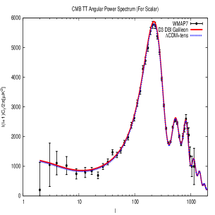
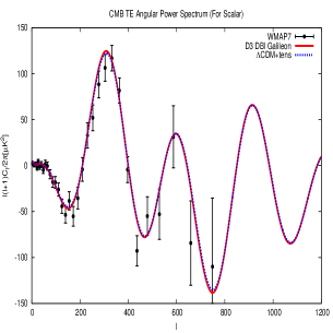
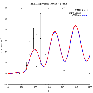
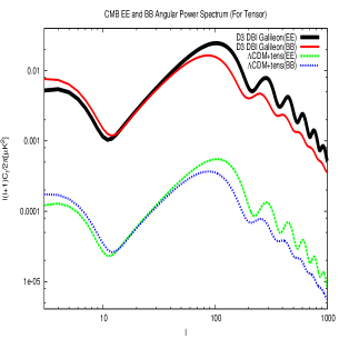
DBI Galileon inflation in background SUGRA

Sayantan Choudhury111Electronic address: sayanphysicsisi@gmail.com and Supratik Pal222Electronic address: supratik@isical.ac.in Physics and Applied Mathematics Unit, Indian Statistical Institute, 203 B.T. Road, Kolkata 700 108, India
Abstract

We introduce a model of potential driven DBI Galileon inflation in background ๐’ฉ๐’ฉ{\cal N}=1, ๐’Ÿ๐’Ÿ{\cal D}=4 SUGRA. Starting from D4-Dโ€‹4ยฏยฏ๐ท4\bar{D4} brane-antibrane in the bulk ๐’ฉ๐’ฉ{\cal N}=2, ๐’Ÿ๐’Ÿ{\cal D}=5 SUGRA including quadratic Gauss-Bonnet corrections, we derive an effective ๐’ฉ๐’ฉ{\cal N}=1, ๐’Ÿ๐’Ÿ{\cal D}=4 SUGRA by dimensional reduction, that results in a Coleman-Weinberg type Galileon potential. We employ this potential in modeling inflation and in subsequent study of primordial quantum fluctuations for scalar and tensor modes. Further, we estimate the major observable parameters in both de Sitter (DS) and beyond de Sitter (BDS) limits and confront them with recent observational data from WMAP7 by using the publicly available code CAMB.

I INTRODUCTION

In the very recent days a good number of theoretical physicists have devoted their attention to the development of consistent modified gravity theories which play analogous role as dark energy or the cosmological constant ratra , caroll . In higher-dimensional setups as in the case of DGP model rdvali ,def where self-acceleration is sourced by a scalar field (the zero helicity mode of the 5D graviton), these types of Infra-Red (IR) modification of gravity nima , gia play a crucial role. Moreover, the DGP model replicates the general relativistic features due to non-linear interactions via the well known Vainshtein mechanism vain ; suji ; babi . Despite its profound success it has got some serious limitations suji , royma , which are resolved by introducing a dynamical field, aka, Galileon espo ; nicolis ; felice arising on the brane from the bulk in the DGP setup. The cosmological consequences of the Galileon models have been studied to some extent in fabio ; chow ; kobayashi ; ajtoll . Very recently, a natural extension to the scenario has been brought forward by tagging Galileon with the good old DBI model guss , edmu , resulting in so-called โ€œDBI Galileonโ€ claudia ; trodden ; goon ; shun ; sebar , that has reflected a rich structure from four dimensional cosmological point of view. However, in most of the physical situations, this type of effective gravity theories are plagued with additional degrees of freedom which often results in unwanted debris like ghosts, Laplacian instabilities etc de ; dec1 ; feli . Very recently a nobel effort towards the supersymmetric extension of the DBI Galileon model and its inflationary signature are discussed in sazi and gaziql . In the present paper we introduce a single scalar field model described by the D3 DBI Galileon originated from D4-Dโ€‹4ยฏยฏ๐ท4\bar{D4} brane anti-brane setup in the background of five dimensional local version of the supersymmetric theory (supergravity). This prevents the framework from having extra degrees of freedom as well as Ostrogradski instabilities ost , resulting in a higher-order derivative scalar field theory free from any such unwanted instabilities. Nevertheless, a consistent field theoretic derivation of the effective potential commonly used in the context of DBI Galileon cosmology has not been brought forth so far. On top of that, it is imperative to point out that the SUGRA origin of D3 DBI Galileon is yet to be addressed. In this article we plan to address both of these issues explicitly by deriving the inflaton potential from our proposed framework of DBI Galileon. It turns out that the derived action includes, in certain limits, the decoupling limit of DGP model as well as some consistent theories of massive gravity; and it also includes the โ€œK-mouflageโ€ zio , zioa and also โ€œG/KGBโ€ inflation kobayashi , yama ; kamada ; vik . Moreover, in general appearance of non-vanishing frame functions in the 4D action expedites breakdown of shift symmetry. Without shift symmetry, it may happen that the theory is unstable against large renormalization. The background action chosen in our model preserves shift symmetry of the single scalar field which gives it a firm footing from phenomenological point of view as well.

The plan of the paper is as follows. First we propose a fairly general framework by taking the full DBI action in D4 brane in the background of bulk ๐’ฉ๐’ฉ{\cal N}=2, ๐’Ÿ๐’Ÿ{\cal D}=5 supergravity sayan1 ; sayan2 ; sayan6 ; nills including the quadratic modification in Einsteinโ€™s Hilbert action via Gauss-Bonnet correction in the bulk coming from two loop correction in string theory sayan19 . Hence, using dimensional reduction technique, we derive the effective action for DBI Galileon in D3 brane in the background of ๐’ฉ๐’ฉ{\cal N}=1, ๐’Ÿ๐’Ÿ{\cal D}=4 supergravity induced by the quadratic correction in the geometry sector and study cosmological inflationary scenario therefrom. We next engage ourselves in studying quantum fluctuations, by employing second order perturbative action for scalar and tensor modes in de Sitter (DS) and beyond de Sitter (BDS) limits, and hence calculate the primordial power spectrum of the scalar and tensor modes, their running and other observable parameters. We further confront our model with observations by using the publicly available code CAMB camb , and find them to fit well with latest observational data from WMAP7wmap7 and expected to fit fair well with upcoming data from PLANCKplanck .

II The Background Action

Let us demonstrate briefly the construction of DBI Galileon starting from ๐’ฉ๐’ฉ{\cal N}=2,๐’Ÿ๐’Ÿ{\cal D}=5 SUGRA along with Gauss Bonnet correction in D4 brane set up. The full five dimensional model is described by the following action

STโ€‹oโ€‹tโ€‹aโ€‹l(5)=SEโ€‹H(5)+SGโ€‹B(5)+SDโ€‹4โ€‹bโ€‹rโ€‹aโ€‹nโ€‹e(5)+SBโ€‹uโ€‹lโ€‹kโ€‹Sโ€‹uโ€‹gโ€‹rโ€‹a(5)subscriptsuperscript๐‘†5๐‘‡๐‘œ๐‘ก๐‘Ž๐‘™subscriptsuperscript๐‘†5๐ธ๐ปsubscriptsuperscript๐‘†5๐บ๐ตsubscriptsuperscript๐‘†5๐ท4๐‘๐‘Ÿ๐‘Ž๐‘›๐‘’subscriptsuperscript๐‘†5๐ต๐‘ข๐‘™๐‘˜๐‘†๐‘ข๐‘”๐‘Ÿ๐‘ŽS^{(5)}_{Total}=S^{(5)}_{EH}+S^{(5)}_{GB}+S^{(5)}_{D4~{}brane}+S^{(5)}_{BulkSugra} (1)

where

SEโ€‹H(5)=12โ€‹ฮบ52โ€‹โˆซd5โ€‹xโ€‹โˆ’g(5)โ€‹[R(5)โˆ’2โ€‹ฮ›5],subscriptsuperscript๐‘†5๐ธ๐ป12subscriptsuperscript๐œ…25superscript๐‘‘5๐‘ฅsuperscript๐‘”5delimited-[]subscript๐‘…52subscriptฮ›5S^{(5)}_{EH}=\frac{1}{2\kappa^{2}_{5}}\int d^{5}x\sqrt{-g^{(5)}}\left[R_{(5)}-2\Lambda_{5}\right], (2)
SGโ€‹B(5)=ฮฑ(5)2โ€‹ฮบ52โ€‹โˆซd5โ€‹xโ€‹โˆ’g(5)โ€‹[RAโ€‹Bโ€‹Cโ€‹Dโ€‹(5)โ€‹RAโ€‹Bโ€‹Cโ€‹D(5)โˆ’4โ€‹RAโ€‹Bโ€‹(5)โ€‹RAโ€‹B(5)+R(5)2]subscriptsuperscript๐‘†5๐บ๐ตsubscript๐›ผ52subscriptsuperscript๐œ…25superscript๐‘‘5๐‘ฅsuperscript๐‘”5delimited-[]superscript๐‘…๐ด๐ต๐ถ๐ท5subscriptsuperscript๐‘…5๐ด๐ต๐ถ๐ท4superscript๐‘…๐ด๐ต5subscriptsuperscript๐‘…5๐ด๐ตsubscriptsuperscript๐‘…25S^{(5)}_{GB}=\frac{\alpha_{(5)}}{2\kappa^{2}_{5}}\int d^{5}x\sqrt{-g^{(5)}}\left[R^{ABCD(5)}R^{(5)}_{ABCD}-4R^{AB(5)}R^{(5)}_{AB}+R^{2}_{(5)}\right] (3)

where ฮฑ(5)subscript๐›ผ5\alpha_{(5)} and ฮบ(5)subscript๐œ…5\kappa_{(5)} represent Gauss-Bonnet coupling and 5D gravitational coupling strength respectively. Additionally, ฮ›(5)subscriptฮ›5\Lambda_{(5)} and g(5)superscript๐‘”5g^{(5)} represent the 5D cosmological constant and the determinant of the 5D metric explicitly mentioned in equation(17). The D4 brane action decomposed into two parts as

SDโ€‹4โ€‹bโ€‹rโ€‹aโ€‹nโ€‹e(5)=SDโ€‹Bโ€‹I(5)+SWโ€‹Z(5),subscriptsuperscript๐‘†5๐ท4๐‘๐‘Ÿ๐‘Ž๐‘›๐‘’subscriptsuperscript๐‘†5๐ท๐ต๐ผsubscriptsuperscript๐‘†5๐‘Š๐‘S^{(5)}_{D4~{}brane}=S^{(5)}_{DBI}+S^{(5)}_{WZ}, (4)

where the DBI action and the Wess-Zumino action are given by respectively

SDโ€‹Bโ€‹I(5)=โˆ’T(4)2โ€‹โˆซd5โ€‹xโ€‹expโก(โˆ’ฮฆ)โ€‹โˆ’(ฮณ(5)+B(5)+2โ€‹ฯ€โ€‹ฮฑโ€ฒโ€‹F(5)),subscriptsuperscript๐‘†5๐ท๐ต๐ผsubscript๐‘‡42superscript๐‘‘5๐‘ฅฮฆsuperscript๐›พ5superscript๐ต52๐œ‹superscript๐›ผโ€ฒsuperscript๐น5S^{(5)}_{DBI}=-\frac{T_{(4)}}{2}\int d^{5}x\exp(-\Phi)\sqrt{-\left(\gamma^{(5)}+B^{(5)}+2\pi\alpha^{{}^{\prime}}F^{(5)}\right)}, (5)
SWโ€‹Z(5)=โˆ’T(4)2โ€‹โˆซโˆ‘n=0,2,4Cn^โˆงexpโก(B^2+2โ€‹ฯ€โ€‹ฮฑโ€ฒโ€‹F2)|4โ€‹fโ€‹oโ€‹rโ€‹m=12โˆซd5xโˆ’g(5){ฯตAโ€‹Bโ€‹Cโ€‹D[โˆ‚AฮฆIโˆ‚BฮฆJ(CIโ€‹Jโ€‹BKโ€‹L4โ€‹T(4)โˆ‚CฮฆKโˆ‚DฮฆL+ฯ€โ€‹ฮฑโ€ฒโ€‹CIโ€‹Jโ€‹FCโ€‹D2+C08โ€‹T(4)BIโ€‹JBKโ€‹Lโˆ‚CฮฆKโˆ‚DฮฆL+ฯ€โ€‹ฮฑโ€ฒโ€‹C02BIโ€‹JFCโ€‹D)+2ฯ€2ฮฑ2โ€ฒT(4)C0FAโ€‹BFCโ€‹Dโˆ’T(4)ฮฝ(ฮฆ)]}\begin{array}[]{lllllll}\displaystyle S^{(5)}_{WZ}=-\frac{T_{(4)}}{2}\int\sum_{n=0,2,4}\hat{C_{n}}\wedge\exp\left(\hat{B}_{2}+2\pi\alpha^{{}^{\prime}}F_{2}\right)|_{4~{}form}\\ ~{}~{}~{}~{}~{}~{}\displaystyle=\frac{1}{2}\int d^{5}x\sqrt{-g^{(5)}}\left\{\epsilon^{ABCD}\left[\partial_{A}\Phi^{I}\partial_{B}\Phi^{J}\left(\frac{C_{IJ}B_{KL}}{4T_{(4)}}\partial_{C}\Phi^{K}\partial_{D}\Phi^{L}+\frac{\pi\alpha^{{}^{\prime}}C_{IJ}F_{CD}}{2}\right.\right.\right.\\ \left.\left.\left.~{}~{}~{}~{}~{}~{}\displaystyle+\frac{C_{0}}{8T_{(4)}}B_{IJ}B_{KL}\partial_{C}\Phi^{K}\partial_{D}\Phi^{L}+\frac{\pi\alpha^{{}^{\prime}}C_{0}}{2}B_{IJ}F_{CD}\right)+2\pi^{2}\alpha^{{}^{\prime}2}T_{(4)}C_{0}F_{AB}F_{CD}-T_{(4)}\nu(\Phi)\right]\right\}\end{array} (6)

where T(4)subscript๐‘‡4T_{(4)} is the D4 brane tension, ฮฑโ€ฒsuperscript๐›ผโ€ฒ\alpha^{{}^{\prime}} is the Regge Slope, expโก(โˆ’ฮฆ)ฮฆ\exp(-\Phi) is the closed string dilaton and C0subscript๐ถ0C_{0} is the Axion. Here and through out the article hat denotes a pull-back onto the D4 brane so that ฮณAโ€‹Bsubscript๐›พ๐ด๐ต\gamma_{AB} is the 5D induced metric on the D4 brane explicitly defined in equation(19). Here ฮณ(5)superscript๐›พ5\gamma^{(5)}, B(5)superscript๐ต5B^{(5)} and F(5)superscript๐น5F^{(5)} represent the determinant of the 5D induced metric (ฮณAโ€‹Bsubscript๐›พ๐ด๐ต\gamma_{AB}) and the gauge fields (BAโ€‹B,FAโ€‹Bsubscript๐ต๐ด๐ตsubscript๐น๐ด๐ตB_{AB},F_{AB}) respectively. The gauge invariant combination of rank 2 field strength tensor, appearing in D4 brane, is โ„ฑAโ€‹B=BAโ€‹B+2โ€‹ฯ€โ€‹ฮฑโ€ฒโ€‹FAโ€‹Bsubscriptโ„ฑ๐ด๐ตsubscript๐ต๐ด๐ต2๐œ‹superscript๐›ผโ€ฒsubscript๐น๐ด๐ต{\cal F}_{AB}=B_{AB}+2\pi\alpha^{{}^{\prime}}F_{AB} and {F2,B2}subscript๐น2subscript๐ต2\{F_{2},B_{2}\} represents 2-form Uโ€‹(1)๐‘ˆ1U(1) gauge fields which have the only non-trivial components along compact direction. On the other hand C4subscript๐ถ4C_{4} has components only along the non-compact spacetime dimensions. In a general flux compactification all fluxes may be turned on as the Ramond-Ramond (RR) forms Fn+1=dโ€‹Cnsubscript๐น๐‘›1๐‘‘subscript๐ถ๐‘›F_{n+1}=dC_{n} (along with their duals) with n=0,2,4๐‘›024n=0,2,4 and the Neveu Schwarz-Neveu Schwarz (NS-NS) flux H3=dโ€‹B2subscript๐ป3๐‘‘subscript๐ต2H_{3}=dB_{2}. Additionally the D4 brane frame function is defined as:

ฮฝโ€‹(ฮฆ)=(ฮฝ0+ฮฝ4ฮฆ4)๐œˆฮฆsubscript๐œˆ0subscript๐œˆ4superscriptฮฆ4\nu(\Phi)=\left(\nu_{0}+\frac{\nu_{4}}{\Phi^{4}}\right) (7)

which is originated from interaction between D4-Dโ€‹4ยฏยฏ๐ท4\bar{D4} brane in string theory. Here ฮฝ0subscript๐œˆ0\nu_{0} and ฮฝ4subscript๐œˆ4\nu_{4} represent the constants characterizing the interaction strength between D4-Dโ€‹4ยฏยฏ๐ท4\bar{D4} brane.

In eqn(1) ๐’ฉ=2,๐’Ÿ=5formulae-sequence๐’ฉ2๐’Ÿ5{\cal N}=2,{\cal D}=5 bulk supergravity action can be written as sayan1 ; sayan2 ; sayan6

SBโ€‹uโ€‹lโ€‹kโ€‹Sโ€‹uโ€‹gโ€‹rโ€‹a(5)=12โ€‹โˆซd5โ€‹xโ€‹โˆ’g(5)โ€‹e(5)โ€‹[โˆ’M53โ€‹R(5)2+i2โ€‹ฮจยฏiโ€‹m~โ€‹ฮ“m~โ€‹n~โ€‹q~โ€‹โˆ‡n~ฮจq~iโˆ’SIโ€‹Jโ€‹Fm~โ€‹n~Iโ€‹FIโ€‹m~โ€‹n~โˆ’12โ€‹gฮผโ€‹ฮฝโ€‹(Dm~โ€‹ฮฆฮผ)โ€‹(Dm~โ€‹ฮฆฮฝ)]+Fermionic+Chernโˆ’Simons+Pauliโ€‹mass,subscriptsuperscript๐‘†5๐ต๐‘ข๐‘™๐‘˜๐‘†๐‘ข๐‘”๐‘Ÿ๐‘Ž12superscript๐‘‘5๐‘ฅsubscript๐‘”5subscript๐‘’5delimited-[]subscriptsuperscript๐‘€35superscript๐‘…52๐‘–2subscriptยฏฮจ๐‘–~๐‘šsuperscriptฮ“~๐‘š~๐‘›~๐‘žsubscriptโˆ‡~๐‘›subscriptsuperscriptฮจ๐‘–~๐‘žsubscript๐‘†๐ผ๐ฝsubscriptsuperscript๐น๐ผ~๐‘š~๐‘›superscript๐น๐ผ~๐‘š~๐‘›12subscript๐‘”๐œ‡๐œˆsubscript๐ท~๐‘šsuperscriptฮฆ๐œ‡superscript๐ท~๐‘šsuperscriptฮฆ๐œˆmissing-subexpressionmissing-subexpressionmissing-subexpressionmissing-subexpressionFermionicChernSimonsPaulimassmissing-subexpressionmissing-subexpressionmissing-subexpressionmissing-subexpression\begin{array}[]{lllll}S^{(5)}_{Bulk~{}Sugra}=\frac{1}{2}\int d^{5}x\sqrt{-g_{(5)}}e_{(5)}\left[-\frac{M^{3}_{5}R^{(5)}}{2}+\frac{i}{2}\bar{\Psi}_{i\tilde{m}}\Gamma^{\tilde{m}\tilde{n}\tilde{q}}\nabla_{\tilde{n}}\Psi^{i}_{\tilde{q}}-{S}_{IJ}F^{I}_{\tilde{m}\tilde{n}}F^{I\tilde{m}\tilde{n}}-\frac{1}{2}g_{\mu\nu}(D_{\tilde{m}}\Phi^{\mu})(D^{\tilde{m}}\Phi^{\nu})\right]\\ \displaystyle~{}~{}~{}~{}~{}~{}~{}~{}~{}~{}~{}~{}~{}~{}~{}~{}~{}~{}~{}~{}~{}~{}~{}~{}~{}~{}~{}~{}~{}~{}~{}~{}~{}~{}~{}~{}~{}~{}~{}~{}~{}~{}~{}~{}~{}~{}~{}~{}~{}~{}~{}~{}~{}~{}~{}~{}~{}~{}~{}~{}~{}~{}~{}~{}~{}~{}~{}~{}~{}~{}~{}~{}~{}~{}~{}~{}~{}~{}+{\rm Fermionic}+{\rm Chern-Simons}+{\rm Pauli~{}~{}mass},\end{array} (8)

The rank-2 tensor field SIโ€‹Jsubscript๐‘†๐ผ๐ฝ{S}_{IJ}, appearing in the kinetic terms of the gauge fields, is the restriction of the metric of the 5 dimensional space on the 4 dimensional manifold of the scalar fields given by

SIโ€‹J=โˆ’2โ€‹CIโ€‹Jโ€‹Kโ€‹hK+3โ€‹hIโ€‹hJ,subscript๐‘†๐ผ๐ฝ2subscript๐ถ๐ผ๐ฝ๐พsuperscriptโ„Ž๐พ3subscriptโ„Ž๐ผsubscriptโ„Ž๐ฝ{S}_{IJ}=-2C_{IJK}h^{K}+3h_{I}h_{J}\;\;, (9)

where hI=CIโ€‹Jโ€‹Kโ€‹hJโ€‹hK=SIโ€‹Jโ€‹hJsubscriptโ„Ž๐ผsubscript๐ถ๐ผ๐ฝ๐พsuperscriptโ„Ž๐ฝsuperscriptโ„Ž๐พsubscript๐‘†๐ผ๐ฝsuperscriptโ„Ž๐ฝ\;h_{I}=C_{IJK}h^{J}h^{K}={S}_{IJ}h^{J}\; and gxโ€‹y=hxIโ€‹hyJโ€‹SIโ€‹Jsubscript๐‘”๐‘ฅ๐‘ฆsuperscriptsubscriptโ„Ž๐‘ฅ๐ผsuperscriptsubscriptโ„Ž๐‘ฆ๐ฝsubscript๐‘†๐ผ๐ฝ\;g_{xy}=h_{x}^{I}h_{y}^{J}{S}_{IJ}\; is the metric of the 444-dimensional manifold โ„ณ4subscriptโ„ณ4{\mathcal{M}}_{4}. In these equations we use hxI=โˆ’32hI,xh_{x}^{I}=-\sqrt{\frac{3}{2}}h^{I},_{x} and hIโ€‹x=32hI,xh_{Ix}=\sqrt{\frac{3}{2}}h_{I},_{x} along with the following constraints

hIโ€‹hI=1,hxIโ€‹hI=hIโ€‹hIโ€‹x=0.formulae-sequencesuperscriptโ„Ž๐ผsubscriptโ„Ž๐ผ1superscriptsubscriptโ„Ž๐‘ฅ๐ผsubscriptโ„Ž๐ผsuperscriptโ„Ž๐ผsubscriptโ„Ž๐ผ๐‘ฅ0h^{I}h_{I}=1,\quad h_{x}^{I}h_{I}=h^{I}h_{Ix}=0\;\;. (10)

Here CIโ€‹Jโ€‹Ksubscript๐ถ๐ผ๐ฝ๐พC_{IJK} are constants symmetric in the three indices satisfies the cubic constraint relationship CIโ€‹Jโ€‹Kโ€‹hIโ€‹hJโ€‹hK=1subscript๐ถ๐ผ๐ฝ๐พsuperscriptโ„Ž๐ผsuperscriptโ„Ž๐ฝsuperscriptโ„Ž๐พ1C_{IJK}h^{I}h^{J}h^{K}=1. With the parity assignments we have adopted, h0superscriptโ„Ž0h^{0} is even, while hx=ฮฆxsuperscriptโ„Ž๐‘ฅsuperscriptฮฆ๐‘ฅh^{x}=\Phi^{x} are odd. Furthermore on the fixed points where the odd quantities vanish, h0=1superscriptโ„Ž01h^{0}=1. Analogous relations hold for the hIsubscriptโ„Ž๐ผh_{I}โ€™s. In this context the 5-dimensional coordinates XA=(xฮฑ,y)superscript๐‘‹๐ดsuperscript๐‘ฅ๐›ผ๐‘ฆX^{A}=(x^{\alpha},y), where y๐‘ฆy parameterizes the extra dimension compactified on the closed interval [โˆ’ฯ€โ€‹R,+ฯ€โ€‹R]๐œ‹๐‘…๐œ‹๐‘…[-\pi R,+\pi R] and Z2subscript๐‘2Z_{2} symmetry is imposed. We consider 5D Yang Mills SUGRA model which is described by the field content {eฮผ~m~,ฮจฮผ~i,Aฮผ~I,ฮปiโ€‹a,ฮฆx}subscriptsuperscript๐‘’~๐‘š~๐œ‡subscriptsuperscriptฮจ๐‘–~๐œ‡subscriptsuperscript๐ด๐ผ~๐œ‡superscript๐œ†๐‘–๐‘Žsuperscriptฮฆ๐‘ฅ\{e^{\tilde{m}}_{\tilde{\mu}},\Psi^{i}_{\tilde{\mu}},A^{I}_{\tilde{\mu}},\lambda^{ia},\Phi^{x}\} where ฮผ~=(ฮผ,5)~๐œ‡๐œ‡5\tilde{\mu}=\left(\mu,5\right) are curved and m~=(m,5ห™)~๐‘š๐‘šห™5\tilde{m}=\left(m,\dot{5}\right) are flat 5D indices with ฮผ,m๐œ‡๐‘š\mu,m their corresponding 4D indices. The remaining indices are I=0,1,โ€ฆ..,nI=0,1,.....,n, a=1,2,โ€ฆ..,na=1,2,.....,n and x=1,2,โ€ฆ.,nx=1,2,....,n. The SUGRA multiplet consists of the fuยจยจ๐‘ข\ddot{u}nfbien eฮผ~m~subscriptsuperscript๐‘’~๐‘š~๐œ‡e^{\tilde{m}}_{\tilde{\mu}}, two graviphoton Aฮผ~0subscriptsuperscript๐ด0~๐œ‡A^{0}_{\tilde{\mu}} and two gravitini ฮจฮผ~isubscriptsuperscriptฮจ๐‘–~๐œ‡\Psi^{i}_{\tilde{\mu}}, where i=1,2๐‘–12i=1,2 is the simplectic Sโ€‹Uโ€‹(2)R๐‘†๐‘ˆsubscript2๐‘…SU(2)_{R} index. Moreover, there exists n vector multiplets, counting the Yang Mills fields (Aฮผ~asubscriptsuperscript๐ด๐‘Ž~๐œ‡A^{a}_{\tilde{\mu}}). The spinor and the scalar fields included in the vector multiplets are collectively denoted by ฮปiโ€‹asuperscript๐œ†๐‘–๐‘Ž\lambda^{ia}, ฮฆxsuperscriptฮฆ๐‘ฅ\Phi^{x} respectively. The indices a and x are flat and curved indices respectively of the 5D manifold โ„ณโ„ณ{\cal M}. It is important to mention here that the Chern-Simons terms can be gauged away assuming cubic constraints and Z2subscript๐‘2Z_{2} symmetry. Now we consider full particle spectrum , the Z2subscript๐‘2Z_{2} even fields {eฮผm,e55ห™,ฮจฮผ1,ฮจ52,A50,Aฮผa,ฮป1โ€‹a}subscriptsuperscript๐‘’๐‘š๐œ‡subscriptsuperscript๐‘’ห™55subscriptsuperscriptฮจ1๐œ‡subscriptsuperscriptฮจ25subscriptsuperscript๐ด05subscriptsuperscript๐ด๐‘Ž๐œ‡superscript๐œ†1๐‘Ž\{e^{m}_{\mu},e^{\dot{5}}_{5},\Psi^{1}_{\mu},\Psi^{2}_{5},A^{0}_{5},A^{a}_{\mu},\lambda^{1a}\} and the Z2subscript๐‘2Z_{2} odd fields {eฮผ5ห™,e5m,ฮจฮผ2,ฮจ51,Aฮผ0,A5a,ฮป2โ€‹a,ฮฆx}subscriptsuperscript๐‘’ห™5๐œ‡subscriptsuperscript๐‘’๐‘š5subscriptsuperscriptฮจ2๐œ‡subscriptsuperscriptฮจ15subscriptsuperscript๐ด0๐œ‡subscriptsuperscript๐ด๐‘Ž5superscript๐œ†2๐‘Žsuperscriptฮฆ๐‘ฅ\{e^{\dot{5}}_{\mu},e^{m}_{5},\Psi^{2}_{\mu},\Psi^{1}_{5},A^{0}_{\mu},A^{a}_{5},\lambda^{2a},\Phi^{x}\} propagates in the bulk. For computational purpose it is useful to define the five dimensional generating function(G๐บG) of supergravity in this setup as

G=โˆ’3โ€‹lnโก(T+Tโ€ 2)+Kโ€‹(ฮฆ,ฮฆโ€ ),๐บ3๐‘‡superscript๐‘‡โ€ 2๐พฮฆsuperscriptฮฆโ€ G=-3\ln\left(\frac{T+T^{\dagger}}{\sqrt{2}}\right)+K(\Phi,\Phi^{\dagger}), (11)

where the supergravity Kaยจยจ๐‘Ž\ddot{a}hler moduli fields are given by

T=(e55ห™โˆ’iโ€‹23โ€‹A50)2๐‘‡subscriptsuperscript๐‘’ห™55๐‘–23subscriptsuperscript๐ด052T=\frac{(e^{\dot{5}}_{5}-i\sqrt{\frac{2}{3}}A^{0}_{5})}{\sqrt{2}} (12)

which is assumed to be stabilized under first approximation and Kโ€‹(ฮฆ,ฮฆโ€ )๐พฮฆsuperscriptฮฆโ€ K(\Phi,\Phi^{\dagger}) represents generalized Kaยจยจ๐‘Ž\ddot{a}hler function.

Including the kinetic term of the five dimensional field ฮฆฮฆ\Phi and rearranging into a perfect square, the 5D bulk supergravity action can be expressed as

SโŠƒ12โˆซd4xโˆซโˆ’ฯ€โ€‹R+ฯ€โ€‹Rdyโˆ’g5e(4)e5ห™5[gฮฑโ€‹ฮฒGMN(โˆ‚ฮฑฮฆM)โ€ (โˆ‚ฮฒฮฆN)+1g55(โˆ‚5ฮฆโˆ’Vbโ€‹uโ€‹lโ€‹k(5)โ€‹(G)))2],S\supset\frac{1}{2}\int d^{4}x\int^{+\pi R}_{-\pi R}dy\sqrt{-g_{5}}e_{(4)}e^{5}_{\dot{5}}\left[g^{\alpha\beta}G_{M}^{N}(\partial_{\alpha}\Phi^{M})^{\dagger}(\partial_{\beta}\Phi_{N})+\frac{1}{g_{55}}\left(\partial_{5}\Phi-\sqrt{V^{(5)}_{bulk}(G)})\right)^{2}\right], (13)

where the 5D potential described by

Vbโ€‹uโ€‹lโ€‹k(5)โ€‹(G)=expโก(GM2)โ€‹[(โˆ‚Wโˆ‚ฮฆM+โˆ‚Gโˆ‚ฮฆMโ€‹WM2)โ€ โ€‹(GMN)โˆ’1โ€‹(โˆ‚Wโˆ‚ฮฆN+โˆ‚Gโˆ‚ฮฆNโ€‹WM2)โˆ’3โ€‹|W|2M2]subscriptsuperscript๐‘‰5๐‘๐‘ข๐‘™๐‘˜๐บ๐บsuperscript๐‘€2delimited-[]superscript๐‘Šsubscriptฮฆ๐‘€๐บsubscriptฮฆ๐‘€๐‘Šsuperscript๐‘€2โ€ superscriptsuperscriptsubscript๐บ๐‘€๐‘1๐‘Šsuperscriptฮฆ๐‘๐บsuperscriptฮฆ๐‘๐‘Šsuperscript๐‘€23superscript๐‘Š2superscript๐‘€2V^{(5)}_{bulk}(G)=\exp\left(\frac{G}{M^{2}}\right)\left[\left(\frac{\partial W}{\partial\Phi_{M}}+\frac{\partial G}{\partial\Phi_{M}}\frac{W}{M^{2}}\right)^{\dagger}(G_{M}^{N})^{-1}\left(\frac{\partial W}{\partial\Phi^{N}}+\frac{\partial G}{\partial\Phi^{N}}\frac{W}{M^{2}}\right)-3\frac{|W|^{2}}{M^{2}}\right] (14)

where W๐‘ŠW physically represents the superpotential in the context of ๐’ฉ=2,๐’Ÿ=5formulae-sequence๐’ฉ2๐’Ÿ5{\cal N}=2,{\cal D}=5 supergravity theory and expressed in terms of the holomorphic combination of the fields ฮฆ,ฮฆโ€ ,Tฮฆsuperscriptฮฆโ€ ๐‘‡\Phi,\Phi^{\dagger},T and Tโ€ superscript๐‘‡โ€ T^{\dagger}. The field equations in presence of Gauss-Bonnet term can be expressed as

GAโ€‹B(5)+ฮฑ(5)โ€‹HAโ€‹B(5)=8โ€‹ฯ€โ€‹G(5)โ€‹TAโ€‹B(5)โˆ’ฮ›(5)โ€‹gAโ€‹B(5),subscriptsuperscript๐บ5๐ด๐ตsubscript๐›ผ5subscriptsuperscript๐ป5๐ด๐ต8๐œ‹subscript๐บ5subscriptsuperscript๐‘‡5๐ด๐ตsubscriptฮ›5subscriptsuperscript๐‘”5๐ด๐ตG^{(5)}_{AB}+\alpha_{(5)}H^{(5)}_{AB}=8\pi G_{(5)}T^{(5)}_{AB}-\Lambda_{(5)}g^{(5)}_{AB}, (15)

where the covariantly conserved Gauss-Bonnet tensor

HAโ€‹B(5)=2โ€‹RAโ€‹Cโ€‹Dโ€‹E(5)โ€‹RBCโ€‹Dโ€‹Eโ€‹(5)โˆ’4โ€‹RAโ€‹Cโ€‹Bโ€‹D(5)โ€‹RCโ€‹Dโ€‹(5)โˆ’4โ€‹RAโ€‹C(5)โ€‹RBCโ€‹(5)+2โ€‹R(5)โ€‹RAโ€‹B(5)โˆ’12โ€‹gAโ€‹B(5)โ€‹(RAโ€‹Bโ€‹Cโ€‹Dโ€‹(5)โ€‹RAโ€‹Bโ€‹Cโ€‹D(5)โˆ’4โ€‹RAโ€‹Bโ€‹(5)โ€‹RAโ€‹B(5)+R(5)2)subscriptsuperscript๐ป5๐ด๐ต2subscriptsuperscript๐‘…5๐ด๐ถ๐ท๐ธsuperscriptsubscript๐‘…๐ต๐ถ๐ท๐ธ54superscriptsubscript๐‘…๐ด๐ถ๐ต๐ท5superscript๐‘…๐ถ๐ท54superscriptsubscript๐‘…๐ด๐ถ5superscriptsubscript๐‘…๐ต๐ถ52superscript๐‘…5superscriptsubscript๐‘…๐ด๐ต512subscriptsuperscript๐‘”5๐ด๐ตsuperscript๐‘…๐ด๐ต๐ถ๐ท5subscriptsuperscript๐‘…5๐ด๐ต๐ถ๐ท4superscript๐‘…๐ด๐ต5subscriptsuperscript๐‘…5๐ด๐ตsubscriptsuperscript๐‘…25H^{(5)}_{AB}=2R^{(5)}_{ACDE}R_{B}^{CDE(5)}-4R_{ACBD}^{(5)}R^{CD(5)}-4R_{AC}^{(5)}R_{B}^{C(5)}+2R^{(5)}R_{AB}^{(5)}-\frac{1}{2}g^{(5)}_{AB}\left(R^{ABCD(5)}R^{(5)}_{ABCD}-4R^{AB(5)}R^{(5)}_{AB}+R^{2}_{(5)}\right) (16)

which acts as a source term. It is useful to introduce the 5D metric in conformal form

dโ€‹s4+12=gAโ€‹Bโ€‹dโ€‹XAโ€‹dโ€‹XB=1hโ€‹(y)โ€‹dโ€‹s42+hโ€‹(y)โ€‹G~โ€‹(y)โ€‹dโ€‹y2=expโก(2โ€‹Aโ€‹(y))โ€‹(dโ€‹s42+R2โ€‹ฮฒ2โ€‹dโ€‹y2),๐‘‘subscriptsuperscript๐‘ 241subscript๐‘”๐ด๐ต๐‘‘superscript๐‘‹๐ด๐‘‘superscript๐‘‹๐ต1โ„Ž๐‘ฆ๐‘‘subscriptsuperscript๐‘ 24โ„Ž๐‘ฆ~๐บ๐‘ฆ๐‘‘superscript๐‘ฆ22๐ด๐‘ฆ๐‘‘subscriptsuperscript๐‘ 24superscript๐‘…2superscript๐›ฝ2๐‘‘superscript๐‘ฆ2ds^{2}_{4+1}=g_{AB}dX^{A}dX^{B}=\frac{1}{\sqrt{h(y)}}ds^{2}_{4}+\sqrt{h(y)}\tilde{G}(y)dy^{2}=\exp(2A(y))\left(ds^{2}_{4}+R^{2}\beta^{2}dy^{2}\right), (17)

with warp factor

expโก(2โ€‹Aโ€‹(y))=1hโ€‹(y)=R2b02โ€‹ฮฒ2โ€‹G~โ€‹(y)=b02R2โ€‹(expโก(ฮฒโ€‹y)+ฮ›(5)โ€‹b0424โ€‹R2โ€‹expโก(โˆ’ฮฒโ€‹y))2๐ด๐‘ฆ1โ„Ž๐‘ฆsuperscript๐‘…2subscriptsuperscript๐‘20superscript๐›ฝ2~๐บ๐‘ฆsubscriptsuperscript๐‘20superscript๐‘…2๐›ฝ๐‘ฆsubscriptฮ›5subscriptsuperscript๐‘4024superscript๐‘…2๐›ฝ๐‘ฆ\exp(2A(y))=\frac{1}{\sqrt{h(y)}}=\frac{R^{2}}{b^{2}_{0}\beta^{2}}\tilde{G}(y)=\frac{b^{2}_{0}}{R^{2}\left(\exp(\beta y)+\frac{\Lambda_{(5)}b^{4}_{0}}{24R^{2}}\exp(-\beta y)\right)} (18)

and dโ€‹s42=gฮฑโ€‹ฮฒโ€‹dโ€‹xฮฑโ€‹dโ€‹xฮฒ๐‘‘subscriptsuperscript๐‘ 24subscript๐‘”๐›ผ๐›ฝ๐‘‘superscript๐‘ฅ๐›ผ๐‘‘superscript๐‘ฅ๐›ฝds^{2}_{4}=g_{\alpha\beta}dx^{\alpha}dx^{\beta} is FLRW counterpart. In order to write down explicitly the expression for D4 brane action, the induced metric can be shown as

ฮณCโ€‹D=1hโ€‹(y)โ€‹(gAโ€‹B+hโ€‹(y)โ€‹G~Aโ€‹Bโ€‹โˆ‚CฮฆAโ€‹โˆ‚DฮฆB).subscript๐›พ๐ถ๐ท1โ„Ž๐‘ฆsubscript๐‘”๐ด๐ตโ„Ž๐‘ฆsubscript~๐บ๐ด๐ตsubscript๐ถsuperscriptฮฆ๐ดsubscript๐ทsuperscriptฮฆ๐ต\gamma_{CD}=\frac{1}{\sqrt{h(y)}}\left(g_{AB}+h(y)\tilde{G}_{AB}\partial_{C}\Phi^{A}\partial_{D}\Phi^{B}\right). (19)

The 5D energy momentum tensor for the set up reads

Tฮฑโ€‹ฮฒtโ€‹oโ€‹tโ€‹aโ€‹lโ€‹(5)=Tฮฑโ€‹ฮฒbโ€‹uโ€‹lโ€‹kโ€‹(5)+Tฮฑโ€‹ฮฒDโ€‹4โ€‹bโ€‹rโ€‹aโ€‹nโ€‹eโ€‹(5)=GMNโ€‹(โˆ‚ฮฑฮฆM)โ€ โ€‹(โˆ‚ฮฒฮฆN)โˆ’gฮฑโ€‹ฮฒโ€‹[gฯโ€‹ฯƒโ€‹(โˆ‚ฯฮฆM)โ€ โ€‹(โˆ‚ฯƒฮฆN)โ€‹GMN+g55โ€‹(โˆ‚5ฮฆโˆ’Vbโ€‹uโ€‹lโ€‹k(5)โ€‹(G))2]+[KMโ€‹N;Xโˆ‚ฮฑฮฆMโˆ‚ฮฒฮฆN+Kgฮฑโ€‹ฮฒโˆ’2โˆ‡(ฮฑG(ฮฆ,X)โˆ‡ฮฒ)ฮฆ+gฮฑโ€‹ฮฒโˆ‚ฮปG(ฮฆ,X)โˆ‚ฮปฮฆโˆ’GMโ€‹N;X(ฮฆ,X)โ–กฮฆโˆ‚ฮฑฮฆMโˆ‚ฮฒฮฆN],\begin{array}[]{lllllll}T^{total(5)}_{\alpha\beta}=T^{bulk(5)}_{\alpha\beta}+T^{D4brane(5)}_{\alpha\beta}=G^{N}_{M}(\partial_{\alpha}\Phi^{M})^{\dagger}(\partial_{\beta}\Phi_{N})-g_{\alpha\beta}\left[g^{\rho\sigma}(\partial_{\rho}\Phi^{M})^{\dagger}(\partial_{\sigma}\Phi_{N})G^{N}_{M}+g^{55}\left(\partial_{5}\Phi-\sqrt{V^{(5)}_{bulk}(G)}\right)^{2}\right]\\ ~{}~{}~{}~{}~{}~{}~{}~{}~{}~{}~{}~{}~{}~{}~{}~{}~{}~{}~{}~{}~{}~{}~{}~{}~{}~{}~{}~{}~{}~{}~{}~{}~{}~{}~{}~{}~{}~{}~{}~{}~{}~{}~{}~{}~{}~{}~{}+\left[K_{MN;X}\partial_{\alpha}\Phi^{M}\partial_{\beta}\Phi^{N}+Kg_{\alpha\beta}-2\nabla_{(\alpha}G(\Phi,X)\nabla_{\beta)}\Phi+g_{\alpha\beta}\partial_{\lambda}G(\Phi,X)\partial^{\lambda}\Phi\right.\\ \left.~{}~{}~{}~{}~{}~{}~{}~{}~{}~{}~{}~{}~{}~{}~{}~{}~{}~{}~{}~{}~{}~{}~{}~{}~{}~{}~{}~{}~{}~{}~{}~{}~{}~{}~{}~{}~{}~{}~{}~{}~{}~{}~{}~{}~{}~{}~{}~{}~{}~{}~{}~{}~{}~{}~{}~{}~{}~{}~{}~{}~{}~{}~{}~{}~{}~{}~{}~{}~{}~{}~{}~{}~{}~{}~{}~{}~{}~{}~{}~{}-G_{MN;X}(\Phi,X)\Box\Phi\partial_{\alpha}\Phi^{M}\partial_{\beta}\Phi^{N}\right],\end{array} (20)
T55tโ€‹oโ€‹tโ€‹aโ€‹lโ€‹(5)=T55bโ€‹uโ€‹lโ€‹kโ€‹(5)+T55Dโ€‹4โ€‹bโ€‹rโ€‹aโ€‹nโ€‹eโ€‹(5)=12โ€‹(โˆ‚5ฮฆโˆ’Vbโ€‹uโ€‹lโ€‹k(5)โ€‹(G))2โˆ’12โ€‹g55โ€‹gฯโ€‹ฯƒโ€‹GMNโ€‹(โˆ‚ฯฮฆM)โ€ โ€‹(โˆ‚ฯƒฮฆN)+[KMโ€‹N;Xโˆ‚5ฮฆMโˆ‚5ฮฆN+Kg55โˆ’2โˆ‡(5G(ฮฆ,X)โˆ‡5)ฮฆ+g55โˆ‚ฮปG(ฮฆ,X)โˆ‚ฮปฮฆโˆ’GMโ€‹N;X(ฮฆ,X)โ–กฮฆโˆ‚5ฮฆMโˆ‚5ฮฆN].\begin{array}[]{llllll}T^{total(5)}_{55}=T^{bulk(5)}_{55}+T^{D4brane(5)}_{55}=\frac{1}{2}\left(\partial_{5}\Phi-\sqrt{V^{(5)}_{bulk}(G)}\right)^{2}-\frac{1}{2}g_{55}g^{\rho\sigma}G^{N}_{M}(\partial_{\rho}\Phi^{M})^{\dagger}(\partial_{\sigma}\Phi_{N})\\ ~{}~{}~{}~{}~{}~{}~{}~{}~{}~{}~{}~{}~{}~{}~{}~{}~{}~{}~{}~{}~{}~{}~{}~{}~{}~{}~{}~{}~{}~{}~{}~{}~{}~{}~{}~{}~{}~{}~{}~{}~{}~{}~{}~{}~{}~{}~{}+\left[K_{MN;X}\partial_{5}\Phi^{M}\partial_{5}\Phi^{N}+Kg_{55}-2\nabla_{(5}G(\Phi,X)\nabla_{5)}\Phi+g_{55}\partial_{\lambda}G(\Phi,X)\partial^{\lambda}\Phi\right.\\ \left.~{}~{}~{}~{}~{}~{}~{}~{}~{}~{}~{}~{}~{}~{}~{}~{}~{}~{}~{}~{}~{}~{}~{}~{}~{}~{}~{}~{}~{}~{}~{}~{}~{}~{}~{}~{}~{}~{}~{}~{}~{}~{}~{}~{}~{}~{}~{}~{}~{}~{}~{}~{}~{}~{}~{}~{}~{}~{}~{}~{}~{}~{}~{}~{}~{}~{}~{}~{}~{}~{}~{}~{}~{}~{}~{}~{}~{}~{}~{}~{}-G_{MN;X}(\Phi,X)\Box\Phi\partial_{5}\Phi^{M}\partial_{5}\Phi^{N}\right].\end{array} (21)

On the other hand, the Klein-Gordon equation of motion in 5D can be expressed as

โˆ‚5[e5ห™5โ€‹g5g55โ€‹(โˆ‚5ฮฆโˆ’Vbโ€‹uโ€‹lโ€‹k(5)โ€‹(G))]+โˆ‘Ne5ห™5โ€‹{โˆ‚ฮฒ[g5โ€‹gฮฑโ€‹ฮฒโ€‹GMNโ€‹(โˆ‚ฮฑฮฆM)]โˆ’g5g55โ€‹โˆ‚N(Vbโ€‹uโ€‹lโ€‹k(5)โ€‹(G))โ€‹(โˆ‚5ฮฆโˆ’Vbโ€‹uโ€‹lโ€‹k(5)โ€‹(G))}KXโ€‹(ฮฆ,X)โ€‹โ–ก(5)โ€‹ฮฆโˆ’KXโ€‹Xโ€‹(ฮฆ,X)โ€‹(โˆ‡Aโˆ‡Bโกฮฆ)โ€‹(โˆ‡Aฮฆโ€‹โˆ‡Bฮฆ)โˆ’2โ€‹Kฮฆโ€‹Xโ€‹(ฮฆ,X)โ€‹X+Kฮฆโ€‹(ฮฆ,X)โˆ’2โ€‹(Gฮฆโ€‹(ฮฆ,X)โˆ’Gฮฆโ€‹Xโ€‹(ฮฆ,X)โ€‹X)+GXโ€‹(ฮฆ,X)โ€‹[(โˆ‡Aโˆ‡Bโกฮฆ)โ€‹(โˆ‡Aโˆ‡Bโกฮฆ)โˆ’(โ–ก(5)โ€‹ฮฆ)2+RAโ€‹B(5)โ€‹โˆ‡Aฮฆโ€‹โˆ‡Bฮฆ]+2โ€‹Gฮฆโ€‹Xโ€‹(ฮฆ,X)โ€‹(โˆ‡Aโˆ‡Bโกฮฆ)โ€‹(โˆ‡Aโˆ‡Bโกฮฆ)+2โ€‹Gฮฆโ€‹ฮฆโ€‹(ฮฆ,X)โ€‹Xโˆ’GXโ€‹Xโ€‹(โˆ‡Aโˆ‡Bโกฮฆโˆ’gAโ€‹Bโ€‹โ–ก(5)โ€‹ฮฆ)โ€‹(โˆ‡Aโˆ‡Cโกฮฆ)โ€‹(โˆ‡Bฮฆ)โ€‹(โˆ‡Cฮฆ)=0.subscript5delimited-[]subscriptsuperscript๐‘’5ห™5subscript๐‘”5subscript๐‘”55subscript5ฮฆsubscriptsuperscript๐‘‰5๐‘๐‘ข๐‘™๐‘˜๐บsubscript๐‘subscriptsuperscript๐‘’5ห™5subscript๐›ฝdelimited-[]subscript๐‘”5superscript๐‘”๐›ผ๐›ฝsubscriptsuperscript๐บ๐‘๐‘€subscript๐›ผsuperscriptฮฆ๐‘€subscript๐‘”5subscript๐‘”55subscript๐‘subscriptsuperscript๐‘‰5๐‘๐‘ข๐‘™๐‘˜๐บsubscript5ฮฆsubscriptsuperscript๐‘‰5๐‘๐‘ข๐‘™๐‘˜๐บmissing-subexpressionmissing-subexpressionmissing-subexpressionmissing-subexpressionmissing-subexpressionsubscript๐พ๐‘‹ฮฆ๐‘‹superscriptโ–ก5ฮฆsubscript๐พ๐‘‹๐‘‹ฮฆ๐‘‹subscriptโˆ‡๐ดsubscriptโˆ‡๐ตฮฆsuperscriptโˆ‡๐ดฮฆsuperscriptโˆ‡๐ตฮฆ2subscript๐พฮฆ๐‘‹ฮฆ๐‘‹๐‘‹subscript๐พฮฆฮฆ๐‘‹2subscript๐บฮฆฮฆ๐‘‹subscript๐บฮฆ๐‘‹ฮฆ๐‘‹๐‘‹missing-subexpressionmissing-subexpressionmissing-subexpressionmissing-subexpressionmissing-subexpressionsubscript๐บ๐‘‹ฮฆ๐‘‹delimited-[]subscriptโˆ‡๐ดsubscriptโˆ‡๐ตฮฆsuperscriptโˆ‡๐ดsuperscriptโˆ‡๐ตฮฆsuperscriptsuperscriptโ–ก5ฮฆ2subscriptsuperscript๐‘…5๐ด๐ตsuperscriptโˆ‡๐ดฮฆsuperscriptโˆ‡๐ตฮฆ2subscript๐บฮฆ๐‘‹ฮฆ๐‘‹subscriptโˆ‡๐ดsubscriptโˆ‡๐ตฮฆsuperscriptโˆ‡๐ดsuperscriptโˆ‡๐ตฮฆ2subscript๐บฮฆฮฆฮฆ๐‘‹๐‘‹missing-subexpressionmissing-subexpressionmissing-subexpressionmissing-subexpressionmissing-subexpressionsubscript๐บ๐‘‹๐‘‹superscriptโˆ‡๐ดsuperscriptโˆ‡๐ตฮฆsuperscript๐‘”๐ด๐ตsuperscriptโ–ก5ฮฆsubscriptโˆ‡๐ดsuperscriptโˆ‡๐ถฮฆsubscriptโˆ‡๐ตฮฆsubscriptโˆ‡๐ถฮฆ0missing-subexpressionmissing-subexpressionmissing-subexpressionmissing-subexpressionmissing-subexpression\begin{array}[]{llllll}\partial_{5}\left[\frac{e^{5}_{\dot{5}}\sqrt{g_{5}}}{g_{55}}\left(\partial_{5}\Phi-\sqrt{V^{(5)}_{bulk}(G)}\right)\right]+\sum_{N}e^{5}_{\dot{5}}\left\{\partial_{\beta}\left[\sqrt{g_{5}}g^{\alpha\beta}G^{N}_{M}(\partial_{\alpha}\Phi^{M})\right]-\frac{\sqrt{g_{5}}}{g_{55}}\partial_{N}\left(\sqrt{V^{(5)}_{bulk}(G)}\right)\left(\partial_{5}\Phi-\sqrt{V^{(5)}_{bulk}(G)}\right)\right\}\\ K_{X}(\Phi,X)\Box^{(5)}\Phi-K_{XX}(\Phi,X)\left(\nabla_{A}\nabla_{B}\Phi\right)\left(\nabla^{A}\Phi\nabla^{B}\Phi\right)-2K_{\Phi X}(\Phi,X)X+K_{\Phi}(\Phi,X)-2\left(G_{\Phi}(\Phi,X)-G_{\Phi X}(\Phi,X)X\right)\\ +G_{X}(\Phi,X)\left[\left(\nabla_{A}\nabla_{B}\Phi\right)\left(\nabla^{A}\nabla^{B}\Phi\right)-\left(\Box^{(5)}\Phi\right)^{2}+R^{(5)}_{AB}\nabla^{A}\Phi\nabla^{B}\Phi\right]+2G_{\Phi X}(\Phi,X)\left(\nabla_{A}\nabla_{B}\Phi\right)\left(\nabla^{A}\nabla^{B}\Phi\right)+2G_{\Phi\Phi}(\Phi,X)X\\ -G_{XX}\left(\nabla^{A}\nabla^{B}\Phi-g^{AB}\Box^{(5)}\Phi\right)\left(\nabla_{A}\nabla^{C}\Phi\right)\left(\nabla_{B}\Phi\right)\left(\nabla_{C}\Phi\right)=0.\end{array} (22)

Now using the scaling relations

ฮฆA=T(4)โ€‹ฮฆ~A,GAโ€‹B=expโก(โˆ’ฮฆ)โ€‹g~Aโ€‹B,bAโ€‹B=hโ€‹(y)T(4)โ€‹BAโ€‹Bformulae-sequencesuperscriptฮฆ๐ดsubscript๐‘‡4superscript~ฮฆ๐ดformulae-sequencesubscript๐บ๐ด๐ตฮฆsubscript~๐‘”๐ด๐ตsubscript๐‘๐ด๐ตโ„Ž๐‘ฆsubscript๐‘‡4subscript๐ต๐ด๐ตmissing-subexpressionmissing-subexpressionmissing-subexpression\begin{array}[]{llll}\displaystyle{\Phi}^{A}=\sqrt{T_{(4)}}\tilde{\Phi}^{A},~{}~{}~{}~{}G_{AB}=\exp(-\Phi)\tilde{g}_{AB},~{}~{}~{}~{}b_{AB}=\frac{\sqrt{h(y)}}{T_{(4)}}B_{AB}\end{array} (23)

the 5D action for D4 brane can be expressed in more convenient form as

SDโ€‹4โ€‹bโ€‹rโ€‹aโ€‹nโ€‹e(5)=โˆซd5โ€‹xโ€‹โˆ’g(5)โ€‹[Kโ€‹(ฮฆ,X)โˆ’Gโ€‹(ฮฆ,X)โ€‹โ–ก(5)โ€‹ฮฆ],subscriptsuperscript๐‘†5๐ท4๐‘๐‘Ÿ๐‘Ž๐‘›๐‘’superscript๐‘‘5๐‘ฅsuperscript๐‘”5delimited-[]๐พฮฆ๐‘‹๐บฮฆ๐‘‹superscriptโ–ก5ฮฆS^{(5)}_{D4~{}brane}=\int d^{5}x\sqrt{-g^{(5)}}\left[K(\Phi,X)-G(\Phi,X)\Box^{(5)}\Phi\right], (24)

where

Kโ€‹(ฮฆ,X)=โˆ’12โ€‹fโ€‹(ฮฆ)โ€‹(๐’Ÿโˆ’1)โˆ’Vbโ€‹rโ€‹aโ€‹nโ€‹e(5)โ€‹(ฮฆ)2๐พฮฆ๐‘‹12๐‘“ฮฆ๐’Ÿ1subscriptsuperscript๐‘‰5๐‘๐‘Ÿ๐‘Ž๐‘›๐‘’ฮฆ2K(\Phi,X)=-\frac{1}{2f(\Phi)}\left(\sqrt{\cal D}-1\right)-\frac{V^{(5)}_{brane}(\Phi)}{2} (25)

where the determinant can be expressed as

๐’Ÿโ‰ƒ1โˆ’2โ€‹fโ€‹(ฮฆ)โ€‹GAโ€‹Bโ€‹XAโ€‹B+4โ€‹f2โ€‹(ฮฆ)โ€‹XA[Aโ€‹XBB]โˆ’8โ€‹f3โ€‹(ฮฆ)โ€‹XA[Aโ€‹XBBโ€‹XCC]+16โ€‹f4โ€‹(ฮฆ)โ€‹XA[Aโ€‹XBBโ€‹XCCโ€‹XDD]{\cal D}\simeq 1-2f(\Phi)G_{AB}X^{AB}+4f^{2}(\Phi)X_{A}^{[A}X_{B}^{B]}-8f^{3}(\Phi)X_{A}^{[A}X^{B}_{B}X^{C]}_{C}+16f^{4}(\Phi)X_{A}^{[A}X^{B}_{B}X^{C}_{C}X^{D]}_{D} (26)

which is expressed in terms of the kinetic term XDB=โˆ’12โ€‹GDโ€‹Aโ€‹โˆ‚CฮฆAโ€‹โˆ‚CฮฆBsubscriptsuperscript๐‘‹๐ต๐ท12subscript๐บ๐ท๐ดsuperscript๐ถsuperscriptฮฆ๐ดsubscript๐ถsuperscriptฮฆ๐ตX^{B}_{D}=-\frac{1}{2}G_{DA}\partial^{C}\Phi^{A}\partial_{C}\Phi^{B}. The detailed calculation for the determinant is elaborately discussed in the Appendex D. In this context the 5D Dโ€™Alembertian Operator is defined as

โ–ก(5)=1โˆ’g(5)โ€‹โˆ‚A(โˆ’g(5)โ€‹gAโ€‹Cโ€‹โˆ‚C).superscriptโ–ก51superscript๐‘”5subscript๐ดsuperscript๐‘”5superscript๐‘”๐ด๐ถsubscript๐ถ\Box^{(5)}=\frac{1}{\sqrt{-g^{(5)}}}\partial_{A}\left(\sqrt{-g^{(5)}}g^{AC}\partial_{C}\right). (27)

Here we use the fact that no spatial direction along which the scalar fields are only time dependent lead to Bฮฝฮผ=0subscriptsuperscript๐ต๐œ‡๐œˆ0B^{\mu}_{\nu}=0 and Fฮผโ€‹ฮฝ=0subscript๐น๐œ‡๐œˆ0F_{\mu\nu}=0 in the background. Consequently Maxwellโ€™s field equations are unaffected in 4D after dimensional reduction. In this context the 5D D4 brane potential is given by

Vbโ€‹rโ€‹aโ€‹nโ€‹e(5)โ€‹(ฮฆ)=T(4)โ€‹ฮฝโ€‹(ฮฆ)+1fโ€‹(ฮฆ),subscriptsuperscript๐‘‰5๐‘๐‘Ÿ๐‘Ž๐‘›๐‘’ฮฆsubscript๐‘‡4๐œˆฮฆ1๐‘“ฮฆV^{(5)}_{brane}(\Phi)=T_{(4)}\nu(\Phi)+\frac{1}{f(\Phi)}, (28)

where 5D warped geometry motivated Z2subscript๐‘2Z_{2} symmetric frame function

fโ€‹(ฮฆ)=expโก(ฮฆ)โ€‹hโ€‹(y)T(4)โ‰ƒ1(f0+f2โ€‹ฮฆ2+f4โ€‹ฮฆ4)๐‘“ฮฆฮฆโ„Ž๐‘ฆsubscript๐‘‡4similar-to-or-equals1subscript๐‘“0subscript๐‘“2superscriptฮฆ2subscript๐‘“4superscriptฮฆ4f(\Phi)=\frac{\exp(\Phi)h(y)}{T_{(4)}}\simeq\frac{1}{(f_{0}+f_{2}\Phi^{2}+f_{4}\Phi^{4})} (29)

is originated from higher dimensional field theory and the implicit D4 brane function defined as:

Gโ€‹(ฮฆ,X)=gโ€‹(ฮฆ)2โ€‹(1โˆ’2โ€‹fโ€‹(ฮฆ)โ€‹X)๐บฮฆ๐‘‹๐‘”ฮฆ212๐‘“ฮฆ๐‘‹G(\Phi,X)=\frac{g(\Phi)}{2(1-2f(\Phi)X)} (30)

with gโ€‹(ฮฆ)=g0+g2โ€‹ฮฆ2๐‘”ฮฆsubscript๐‘”0subscript๐‘”2superscriptฮฆ2g(\Phi)=g_{0}+g_{2}\Phi^{2}. Here g0subscript๐‘”0g_{0} and g2subscript๐‘”2g_{2} are model dependent constants characterizes the effects of possible interactions on the D4 brane.
III Modeling Inflation from D3 DBI Galileon

The technical details of the dimensional reduction technique are elaborately discussed in the Appendix A which can generate an effective D3 DBI Galileon theory in 4D. Now summing up all the contributions from eqn(86), eqn(91), eqn(92) and eqn(99), the model for D3 DBI Galileon is described by the following effective action:

STโ€‹oโ€‹tโ€‹aโ€‹l(4)=โˆซd4xโˆ’g(4)[K~^(ฯ•,X~)โˆ’G~(ฯ•,X~)โ–ก(4)ฯ•+l~1R(4)+l~4(๐’ž(1)Rฮฑโ€‹ฮฒโ€‹ฮณโ€‹ฮดโ€‹(4)Rฮฑโ€‹ฮฒโ€‹ฮณโ€‹ฮด(4)โˆ’4โ„(2)Rฮฑโ€‹ฮฒโ€‹(4)Rฮฑโ€‹ฮฒ(4)+๐’œ(6)R(4)2)+l~3],\begin{array}[]{lllllll}\displaystyle S^{(4)}_{Total}=\int d^{4}x\sqrt{-g^{(4)}}\left[\hat{\tilde{K}}(\phi,\tilde{X})-\tilde{G}(\phi,\tilde{X})\Box^{(4)}\phi+\tilde{l}_{1}R_{(4)}\right.\\ \left.\displaystyle~{}~{}~{}~{}~{}~{}~{}~{}~{}~{}~{}~{}~{}~{}~{}~{}~{}~{}~{}~{}~{}~{}~{}~{}~{}~{}~{}~{}~{}~{}~{}~{}~{}~{}~{}~{}~{}~{}~{}~{}~{}~{}~{}~{}~{}+\tilde{l}_{4}\left({\cal C}(1)R^{\alpha\beta\gamma\delta(4)}R^{(4)}_{\alpha\beta\gamma\delta}-4{\cal I}(2)R^{\alpha\beta(4)}R^{(4)}_{\alpha\beta}+{\cal A}(6)R^{2}_{(4)}\right)+\tilde{l}_{3}\right],\end{array} (31)

where

K~^โ€‹(ฯ•,X~)=K~โ€‹(ฯ•,X~)โˆ’2โ€‹Xโ€‹M~โ€‹(T,Tโ€ )โˆ’Z~โ€‹(T,Tโ€ )โ€‹Vbโ€‹uโ€‹lโ€‹k(4)โ€‹(ฯ•),M~โ€‹(T,Tโ€ )=Mโ€‹(T,Tโ€ )2โ€‹ฮบ(4)2,Z~โ€‹(T,Tโ€ )=Zโ€‹(T,Tโ€ )2โ€‹ฮบ(4)2,l~1={12โ€‹ฮบ(4)2โ€‹[1+ฮฑ(4)R2โ€‹ฮฒ2โ€‹(24โ€‹โ„โ€‹(2)โˆ’24โ€‹๐’œโ€‹(9)โˆ’16โ€‹๐’œโ€‹(10))]โˆ’ฮฑ(4)โ€‹๐’žโ€‹(2)ฮบ(4)2โ€‹R2โ€‹ฮฒ2},l~4=ฮฑ(4)2โ€‹ฮบ(4)2,l~3=12โ€‹ฮบ(4)2โ€‹[ฮฑ(4)R4โ€‹ฮฒ4โ€‹(24โ€‹๐’žโ€‹(24)โˆ’144โ€‹โ„โ€‹(4)โˆ’64โ€‹๐’œโ€‹(5)+144โ€‹๐’œโ€‹(7)+64โ€‹๐’œโ€‹(8)+192โ€‹๐’œโ€‹(11))โˆ’3โ€‹M53โ€‹ฮฒโ€‹b062โ€‹ฮบ(4)2โ€‹MPโ€‹L2โ€‹R5โ€‹โ„โ€‹(1)]^~๐พitalic-ฯ•~๐‘‹~๐พitalic-ฯ•~๐‘‹2๐‘‹~๐‘€๐‘‡superscript๐‘‡โ€ ~๐‘๐‘‡superscript๐‘‡โ€ subscriptsuperscript๐‘‰4๐‘๐‘ข๐‘™๐‘˜italic-ฯ•missing-subexpressionmissing-subexpressionmissing-subexpressionmissing-subexpressionformulae-sequence~๐‘€๐‘‡superscript๐‘‡โ€ ๐‘€๐‘‡superscript๐‘‡โ€ 2subscriptsuperscript๐œ…24~๐‘๐‘‡superscript๐‘‡โ€ ๐‘๐‘‡superscript๐‘‡โ€ 2subscriptsuperscript๐œ…24missing-subexpressionmissing-subexpressionmissing-subexpressionmissing-subexpressionsubscript~๐‘™112subscriptsuperscript๐œ…24delimited-[]1subscript๐›ผ4superscript๐‘…2superscript๐›ฝ224โ„224๐’œ916๐’œ10subscript๐›ผ4๐’ž2subscriptsuperscript๐œ…24superscript๐‘…2superscript๐›ฝ2missing-subexpressionmissing-subexpressionmissing-subexpressionmissing-subexpressionsubscript~๐‘™4subscript๐›ผ42subscriptsuperscript๐œ…24missing-subexpressionmissing-subexpressionmissing-subexpressionmissing-subexpressionsubscript~๐‘™312subscriptsuperscript๐œ…24delimited-[]subscript๐›ผ4superscript๐‘…4superscript๐›ฝ424๐’ž24144โ„464๐’œ5144๐’œ764๐’œ8192๐’œ113subscriptsuperscript๐‘€35๐›ฝsubscriptsuperscript๐‘602subscriptsuperscript๐œ…24subscriptsuperscript๐‘€2๐‘ƒ๐ฟsuperscript๐‘…5โ„1missing-subexpressionmissing-subexpressionmissing-subexpressionmissing-subexpression\begin{array}[]{lllll}\hat{\tilde{K}}(\phi,\tilde{X})=\tilde{K}(\phi,\tilde{X})-2X\tilde{M}(T,T^{{\dagger}})-\tilde{Z}(T,T^{{\dagger}})V^{(4)}_{bulk}(\phi),\\ \tilde{M}(T,T^{{\dagger}})=\frac{M(T,T^{{\dagger}})}{2\kappa^{2}_{(4)}},\tilde{Z}(T,T^{{\dagger}})=\frac{Z(T,T^{{\dagger}})}{2\kappa^{2}_{(4)}},\\ \tilde{l}_{1}=\left\{\frac{1}{2\kappa^{2}_{(4)}}\left[1+\frac{\alpha_{(4)}}{R^{2}\beta^{2}}\left(24{\cal I}(2)-24{\cal A}(9)-16{\cal A}(10)\right)\right]-\frac{\alpha_{(4)}{\cal C}(2)}{\kappa^{2}_{(4)}R^{2}\beta^{2}}\right\},\\ \tilde{l}_{4}=\frac{\alpha_{(4)}}{2\kappa^{2}_{(4)}},\\ \tilde{l}_{3}=\frac{1}{2\kappa^{2}_{(4)}}\left[\frac{\alpha_{(4)}}{R^{4}\beta^{4}}\left(24{\cal C}(24)-144{\cal I}(4)-64{\cal A}(5)+144{\cal A}(7)+64{\cal A}(8)+192{\cal A}(11)\right)-\frac{3M^{3}_{5}\beta b^{6}_{0}}{2\kappa^{2}_{(4)}M^{2}_{PL}R^{5}}{\cal I}(1)\right]\end{array} (32)

where ฮฑ(4)subscript๐›ผ4\alpha_{(4)} and ฮบ(4)subscript๐œ…4\kappa_{(4)} are effective 4D Gauss-Bonnet coupling and gravitational coupling strength. Here X~~๐‘‹\tilde{X} represents the 4D kinetic term after dimensional reduction. The other constants appearing in equation(31) and equation(32) are explicitly mentioned in the Appendix C. For clarity, in terms of the effective potential the total four dimension action for our set up can be rewritten as:

STโ€‹oโ€‹tโ€‹aโ€‹l(4)=โˆซd4xโˆ’g(4)[K(ฯ•,X~)โˆ’G~(ฯ•,X~)โ–ก(4)ฯ•โˆ’V(ฯ•)+l~1R(4)+l~4(๐’ž(1)Rฮฑโ€‹ฮฒโ€‹ฮณโ€‹ฮดโ€‹(4)Rฮฑโ€‹ฮฒโ€‹ฮณโ€‹ฮด(4)โˆ’4โ„(2)Rฮฑโ€‹ฮฒโ€‹(4)Rฮฑโ€‹ฮฒ(4)+๐’œ(6)R(4)2)+l~3],\begin{array}[]{lllllll}\displaystyle S^{(4)}_{Total}=\int d^{4}x\sqrt{-g^{(4)}}\left[K(\phi,\tilde{X})-\tilde{G}(\phi,\tilde{X})\Box^{(4)}\phi-V(\phi)\right.\\ \left.\displaystyle~{}~{}~{}~{}~{}~{}~{}~{}~{}~{}~{}~{}~{}~{}~{}~{}~{}~{}~{}~{}~{}~{}~{}~{}~{}~{}~{}~{}~{}~{}~{}~{}~{}~{}~{}~{}~{}~{}~{}~{}~{}~{}~{}~{}~{}+\tilde{l}_{1}R_{(4)}+\tilde{l}_{4}\left({\cal C}(1)R^{\alpha\beta\gamma\delta(4)}R^{(4)}_{\alpha\beta\gamma\delta}-4{\cal I}(2)R^{\alpha\beta(4)}R^{(4)}_{\alpha\beta}+{\cal A}(6)R^{2}_{(4)}\right)+\tilde{l}_{3}\right],\end{array} (33)

where

Kโ€‹(ฯ•,X~)=โˆ’D~f~โ€‹(ฯ•)โ€‹[1โˆ’2โ€‹Qโ€‹X~โ€‹f~โˆ’Q1]โˆ’C~5โ€‹G~โ€‹(ฯ•,X~)โˆ’2โ€‹Xโ€‹M~โ€‹(T,Tโ€ )๐พitalic-ฯ•~๐‘‹~๐ท~๐‘“italic-ฯ•delimited-[]12๐‘„~๐‘‹~๐‘“subscript๐‘„1subscript~๐ถ5~๐บitalic-ฯ•~๐‘‹2๐‘‹~๐‘€๐‘‡superscript๐‘‡โ€ missing-subexpressionmissing-subexpression\begin{array}[]{lll}\displaystyle K(\phi,\tilde{X})=-\frac{\tilde{D}}{\tilde{f}(\phi)}\left[\sqrt{1-2Q\tilde{X}\tilde{f}}-Q_{1}\right]-\tilde{C}_{5}\tilde{G}(\phi,\tilde{X})-2X\tilde{M}(T,T^{{\dagger}})\end{array} (34)

For details see Appendix A. The collective effect of equation(93) and equation(105) gives the total D3 DBI Galileon potential appearing in equation(33) as:

Vโ€‹(ฯ•)=Qยฏ2โ€‹D~โ€‹Vbโ€‹rโ€‹aโ€‹nโ€‹e(4)+Z~โ€‹(T,Tโ€ )โ€‹Vbโ€‹uโ€‹lโ€‹k(4)โ€‹(ฯ•)=โˆ‘m=โˆ’2,mโ‰ โˆ’12C2โ€‹mโ€‹ฯ•2โ€‹m,๐‘‰italic-ฯ•subscriptยฏ๐‘„2~๐ทsubscriptsuperscript๐‘‰4๐‘๐‘Ÿ๐‘Ž๐‘›๐‘’~๐‘๐‘‡superscript๐‘‡โ€ subscriptsuperscript๐‘‰4๐‘๐‘ข๐‘™๐‘˜italic-ฯ•missing-subexpressionmissing-subexpressionmissing-subexpressionmissing-subexpressionmissing-subexpressionmissing-subexpressionmissing-subexpressionmissing-subexpressionabsentsubscriptsuperscript2formulae-sequence๐‘š2๐‘š1subscript๐ถ2๐‘šsuperscriptitalic-ฯ•2๐‘šmissing-subexpressionmissing-subexpressionmissing-subexpressionmissing-subexpressionmissing-subexpressionmissing-subexpressionmissing-subexpressionmissing-subexpression\begin{array}[]{lllllllll}\displaystyle V(\phi)=\bar{Q}_{2}\tilde{D}V^{(4)}_{brane}+\tilde{Z}(T,T^{{\dagger}})V^{(4)}_{bulk}(\phi)\\ \displaystyle~{}~{}~{}~{}~{}~{}~{}=\sum^{2}_{m=-2,m\neq-1}C_{2m}\phi^{2m},\end{array} (35)

where

C0=(T3โ€‹ฮฝ~0+ฮฒโ€‹Rโ€‹โ„โ€‹(2)โ€‹f~0+Z~โ€‹(T,Tโ€ )โ€‹๐’œโ€‹(13)โ€‹v4),Cโˆ’4=T3โ€‹ฮฝ~4,C2=(ฮฒโ€‹Rโ€‹โ„โ€‹(2)โ€‹f~2โˆ’gโ€‹v2โ€‹Z~โ€‹(T,Tโ€ )โ€‹๐’œโ€‹(13)),C4=(ฮฒโ€‹Rโ€‹โ„โ€‹(2)โ€‹f~4+Z~โ€‹(T,Tโ€ )โ€‹๐’œโ€‹(13)โ€‹g24)subscript๐ถ0subscript๐‘‡3subscript~๐œˆ0๐›ฝ๐‘…โ„2subscript~๐‘“0~๐‘๐‘‡superscript๐‘‡โ€ ๐’œ13superscript๐‘ฃ4missing-subexpressionmissing-subexpressionmissing-subexpressionsubscript๐ถ4subscript๐‘‡3subscript~๐œˆ4missing-subexpressionmissing-subexpressionmissing-subexpressionsubscript๐ถ2๐›ฝ๐‘…โ„2subscript~๐‘“2๐‘”superscript๐‘ฃ2~๐‘๐‘‡superscript๐‘‡โ€ ๐’œ13missing-subexpressionmissing-subexpressionmissing-subexpressionsubscript๐ถ4๐›ฝ๐‘…โ„2subscript~๐‘“4~๐‘๐‘‡superscript๐‘‡โ€ ๐’œ13superscript๐‘”24missing-subexpressionmissing-subexpressionmissing-subexpression\begin{array}[]{llll}\displaystyle C_{0}=\left(T_{3}\tilde{\nu}_{0}+\beta R{\cal I}(2)\tilde{f}_{0}+\tilde{Z}(T,T^{{\dagger}}){\cal A}(13)v^{4}\right),\\ C_{-4}=T_{3}\tilde{\nu}_{4},\\ C_{2}=\left(\beta R{\cal I}(2)\tilde{f}_{2}-gv^{2}\tilde{Z}(T,T^{{\dagger}}){\cal A}(13)\right),\\ C_{4}=\left(\beta R{\cal I}(2)\tilde{f}_{4}+\frac{\tilde{Z}(T,T^{{\dagger}}){\cal A}(13)g^{2}}{4}\right)\end{array} (36)

are tree level constants. Now we want to see the effect of one-loop radiative correction to the derived potential. After doing proper analysis throughout it comes out that the one-loop correction does not effect the superpotential due to the cancellation of all tadpole terms appearing in the theory. On the other hand one-loop radiative correction in the Kaยจยจ๐‘Ž\ddot{a}hler potential results in

ฮดโ€‹๐’ฆ1โˆ’lโ€‹oโ€‹oโ€‹pโ€‹(ฯ•,ฯ•โ€ )=โˆซpฮ›Uโ€‹Vd4โ€‹p(2โ€‹ฯ€)4โ€‹p2โ€‹[12โ€‹Tโ€‹rโ€‹lnโก๐’ฆ^โ€‹(ฯ•,ฯ•โ€ )+12โ€‹Tโ€‹rโ€‹lnโก(๐’ฆ^โ€‹(ฯ•,ฯ•โ€ )โ€‹p2โˆ’๐’ฒ^โ€ โ€‹(ฯ•,ฯ•โ€ )โ€‹(๐’ฆ^โ€‹(ฯ•,ฯ•โ€ )โˆ’1)โ€ โ€‹๐’ฒ^โ€‹(ฯ•,ฯ•โ€ ))]=ฮ›Uโ€‹V216โ€‹ฯ€2โ€‹lnโก(dโ€‹eโ€‹tโ€‹[๐’ฆ^โ€‹(ฯ•,ฯ•โ€ )])โˆ’132โ€‹ฯ€2โ€‹Tโ€‹rโ€‹(โ„ณฯ•2โ€‹[โ„ณฯ•2ฮ›Uโ€‹V2โˆ’1])๐›ฟsuperscript๐’ฆ1๐‘™๐‘œ๐‘œ๐‘italic-ฯ•superscriptitalic-ฯ•โ€ subscriptsuperscriptsubscriptฮ›๐‘ˆ๐‘‰๐‘superscript๐‘‘4๐‘superscript2๐œ‹4superscript๐‘2delimited-[]12๐‘‡๐‘Ÿ^๐’ฆitalic-ฯ•superscriptitalic-ฯ•โ€ 12๐‘‡๐‘Ÿ^๐’ฆitalic-ฯ•superscriptitalic-ฯ•โ€ superscript๐‘2superscript^๐’ฒโ€ italic-ฯ•superscriptitalic-ฯ•โ€ superscript^๐’ฆsuperscriptitalic-ฯ•superscriptitalic-ฯ•โ€ 1โ€ ^๐’ฒitalic-ฯ•superscriptitalic-ฯ•โ€ missing-subexpressionmissing-subexpressionmissing-subexpressionabsentsubscriptsuperscriptฮ›2๐‘ˆ๐‘‰16superscript๐œ‹2๐‘‘๐‘’๐‘กdelimited-[]^๐’ฆitalic-ฯ•superscriptitalic-ฯ•โ€ 132superscript๐œ‹2๐‘‡๐‘Ÿsubscriptsuperscriptโ„ณ2italic-ฯ•delimited-[]subscriptsuperscriptโ„ณ2italic-ฯ•subscriptsuperscriptฮ›2๐‘ˆ๐‘‰1missing-subexpressionmissing-subexpressionmissing-subexpression\begin{array}[]{llll}\displaystyle\delta{\cal K}^{1-loop}(\phi,\phi^{\dagger})=\int^{\Lambda_{UV}}_{p}\frac{d^{4}p}{(2\pi)^{4}p^{2}}\left[\frac{1}{2}Tr\ln\hat{\cal K}(\phi,\phi^{\dagger})+\frac{1}{2}Tr\ln\left(\hat{\cal K}(\phi,\phi^{\dagger})p^{2}-\hat{\cal W}^{\dagger}(\phi,\phi^{\dagger})\left(\hat{\cal K}(\phi,\phi^{\dagger})^{-1}\right)^{\dagger}\hat{\cal W}(\phi,\phi^{\dagger})\right)\right]\\ ~{}~{}~{}~{}~{}~{}~{}~{}~{}~{}~{}~{}~{}~{}~{}~{}~{}~{}~{}~{}\displaystyle=\frac{\Lambda^{2}_{UV}}{16\pi^{2}}\ln\left(det\left[\hat{\cal K}(\phi,\phi^{\dagger})\right]\right)-\frac{1}{32\pi^{2}}Tr\left({\cal M}^{2}_{\phi}\left[\frac{{\cal M}^{2}_{\phi}}{\Lambda^{2}_{UV}}-1\right]\right)\end{array} (37)

where ฮ›Uโ€‹Vsubscriptฮ›๐‘ˆ๐‘‰\Lambda_{UV}(=Mย (Reduced Planck Mass)) is used as a UV cut-off of the theory appearing in the context of cut-off regularization. In this connection the chiral mass matrix is given by

โ„ณฯ•2=๐’ฆ^โˆ’12โ€‹(ฯ•,ฯ•โ€ )โ€‹๐’ฒ^โ€ โ€‹(ฯ•,ฯ•โ€ )โ€‹(๐’ฆ^โ€‹(ฯ•,ฯ•โ€ )โˆ’1)โ€ โ€‹๐’ฒ^โ€‹(ฯ•,ฯ•โ€ )โ€‹๐’ฆ^โˆ’12โ€‹(ฯ•,ฯ•โ€ ).subscriptsuperscriptโ„ณ2italic-ฯ•superscript^๐’ฆ12italic-ฯ•superscriptitalic-ฯ•โ€ superscript^๐’ฒโ€ italic-ฯ•superscriptitalic-ฯ•โ€ superscript^๐’ฆsuperscriptitalic-ฯ•superscriptitalic-ฯ•โ€ 1โ€ ^๐’ฒitalic-ฯ•superscriptitalic-ฯ•โ€ superscript^๐’ฆ12italic-ฯ•superscriptitalic-ฯ•โ€ {\cal M}^{2}_{\phi}=\hat{\cal K}^{-\frac{1}{2}}(\phi,\phi^{\dagger})\hat{\cal W}^{\dagger}(\phi,\phi^{\dagger})\left(\hat{\cal K}(\phi,\phi^{\dagger})^{-1}\right)^{\dagger}\hat{\cal W}(\phi,\phi^{\dagger})\hat{\cal K}^{-\frac{1}{2}}(\phi,\phi^{\dagger}). (38)

Now including the contribution from one-loop radiative correction both from brane and bulk SUGRA, the renormalizable potential is as under

Vโ€‹(ฯ•)=Vtโ€‹rโ€‹eโ€‹eโ€‹(ฯ•)+ฮดโ€‹V1โˆ’lโ€‹oโ€‹oโ€‹pโ€‹(ฯ•)=โˆ‘m=โˆ’2,mโ‰ โˆ’12C2โ€‹mโ€‹ฯ•2โ€‹mโŸTโ€‹rโ€‹eโ€‹eโˆ’lโ€‹eโ€‹vโ€‹eโ€‹lโ€‹cโ€‹oโ€‹nโ€‹tโ€‹rโ€‹iโ€‹bโ€‹uโ€‹tโ€‹iโ€‹oโ€‹n+limฯตโ†’0โˆ‘n=โˆ’2,nโ‰ โˆ’10B2โ€‹mโ€‹(โˆซpฮ›Uโ€‹V=Md4โ€‹p(2โ€‹ฯ€)4โ€‹1(p2โˆ’2โ€‹C2+iโ€‹ฯต)2)โ€‹ฯ•2โ€‹nโŸOโ€‹nโ€‹eโˆ’lโ€‹oโ€‹oโ€‹pโ€‹cโ€‹oโ€‹rโ€‹rโ€‹eโ€‹cโ€‹tโ€‹iโ€‹oโ€‹nโ€‹iโ€‹nโ€‹Dโ€‹3โ€‹bโ€‹rโ€‹aโ€‹nโ€‹e+โˆ‘q=02ฯ•2โ€‹q64โ€‹ฯ€2โ€‹[ฮ›Uโ€‹V4โ€‹Sโ€‹Tโ€‹rโ€‹(โ„ณ0)โ€‹lnโก(ฮ›Uโ€‹V2ฯ•2)+2โ€‹ฮ›Uโ€‹V2โ€‹Sโ€‹Tโ€‹rโ€‹(โ„ณ2)+Sโ€‹Tโ€‹rโ€‹(โ„ณ4โ€‹lnโก(โ„ณ2ฮ›Uโ€‹V2))]โŸOโ€‹nโ€‹eโˆ’lโ€‹oโ€‹oโ€‹pโ€‹cโ€‹oโ€‹rโ€‹rโ€‹eโ€‹cโ€‹tโ€‹iโ€‹oโ€‹nโ€‹iโ€‹nโ€‹tโ€‹hโ€‹eโ€‹bโ€‹uโ€‹lโ€‹kโ€‹๐’ฉ=1,๐’Ÿ=4โ€‹Sโ€‹Uโ€‹Gโ€‹Rโ€‹A=โˆ‘m=โˆ’2,mโ‰ โˆ’12C2โ€‹mโ€‹ฯ•2โ€‹m+โˆ‘n=โˆ’2,nโ‰ โˆ’10Bยฏ2โ€‹nโ€‹lnโก(ฯ•M)โ€‹ฯ•2โ€‹n+โˆ‘q=02A2โ€‹qโ€‹lnโก(ฯ•M)โ€‹ฯ•2โ€‹q=โˆ‘m=โˆ’2,mโ‰ โˆ’12[1+D2โ€‹mโ€‹lnโก(ฯ•M)]โ€‹ฯ•2โ€‹m,๐‘‰italic-ฯ•subscript๐‘‰๐‘ก๐‘Ÿ๐‘’๐‘’italic-ฯ•๐›ฟsubscript๐‘‰1๐‘™๐‘œ๐‘œ๐‘italic-ฯ•missing-subexpressionmissing-subexpressionabsentsubscriptโŸsubscriptsuperscript2formulae-sequence๐‘š2๐‘š1subscript๐ถ2๐‘šsuperscriptitalic-ฯ•2๐‘š๐‘‡๐‘Ÿ๐‘’๐‘’๐‘™๐‘’๐‘ฃ๐‘’๐‘™๐‘๐‘œ๐‘›๐‘ก๐‘Ÿ๐‘–๐‘๐‘ข๐‘ก๐‘–๐‘œ๐‘›subscriptโŸsubscriptโ†’italic-ฯต0subscriptsuperscript0formulae-sequence๐‘›2๐‘›1subscript๐ต2๐‘šsubscriptsuperscriptsubscriptฮ›๐‘ˆ๐‘‰๐‘€๐‘superscript๐‘‘4๐‘superscript2๐œ‹41superscriptsuperscript๐‘22subscript๐ถ2๐‘–italic-ฯต2superscriptitalic-ฯ•2๐‘›๐‘‚๐‘›๐‘’๐‘™๐‘œ๐‘œ๐‘๐‘๐‘œ๐‘Ÿ๐‘Ÿ๐‘’๐‘๐‘ก๐‘–๐‘œ๐‘›๐‘–๐‘›๐ท3๐‘๐‘Ÿ๐‘Ž๐‘›๐‘’missing-subexpressionmissing-subexpressionsubscriptโŸsubscriptsuperscript2๐‘ž0superscriptitalic-ฯ•2๐‘ž64superscript๐œ‹2delimited-[]subscriptsuperscriptฮ›4๐‘ˆ๐‘‰๐‘†๐‘‡๐‘Ÿsuperscriptโ„ณ0subscriptsuperscriptฮ›2๐‘ˆ๐‘‰superscriptitalic-ฯ•22subscriptsuperscriptฮ›2๐‘ˆ๐‘‰๐‘†๐‘‡๐‘Ÿsuperscriptโ„ณ2๐‘†๐‘‡๐‘Ÿsuperscriptโ„ณ4superscriptโ„ณ2subscriptsuperscriptฮ›2๐‘ˆ๐‘‰formulae-sequence๐‘‚๐‘›๐‘’๐‘™๐‘œ๐‘œ๐‘๐‘๐‘œ๐‘Ÿ๐‘Ÿ๐‘’๐‘๐‘ก๐‘–๐‘œ๐‘›๐‘–๐‘›๐‘กโ„Ž๐‘’๐‘๐‘ข๐‘™๐‘˜๐’ฉ1๐’Ÿ4๐‘†๐‘ˆ๐บ๐‘…๐ดmissing-subexpressionmissing-subexpressionabsentsubscriptsuperscript2formulae-sequence๐‘š2๐‘š1subscript๐ถ2๐‘šsuperscriptitalic-ฯ•2๐‘šsubscriptsuperscript0formulae-sequence๐‘›2๐‘›1subscriptยฏ๐ต2๐‘›italic-ฯ•๐‘€superscriptitalic-ฯ•2๐‘›subscriptsuperscript2๐‘ž0subscript๐ด2๐‘žitalic-ฯ•๐‘€superscriptitalic-ฯ•2๐‘žmissing-subexpressionmissing-subexpressionmissing-subexpressionmissing-subexpressionmissing-subexpressionabsentsubscriptsuperscript2formulae-sequence๐‘š2๐‘š1delimited-[]1subscript๐ท2๐‘šitalic-ฯ•๐‘€superscriptitalic-ฯ•2๐‘šmissing-subexpressionmissing-subexpression\begin{array}[]{lll}V(\phi)=V_{tree}(\phi)+\delta V_{1-loop}(\phi)\\ ~{}~{}~{}~{}~{}~{}~{}\displaystyle=\underbrace{\sum^{2}_{m=-2,m\neq-1}C_{2m}\phi^{2m}}_{Tree-level~{}contribution}+\underbrace{\lim_{\epsilon\rightarrow 0}\sum^{0}_{n=-2,n\neq-1}B_{2m}\left(\int^{\Lambda_{UV}=M}_{p}\frac{d^{4}p}{(2\pi)^{4}}\frac{1}{\left(p^{2}-2C_{2}+i\epsilon\right)^{2}}\right)\phi^{2n}}_{One-loop~{}correction~{}in~{}D3~{}brane}\\ ~{}~{}~{}~{}~{}~{}~{}~{}~{}~{}~{}~{}~{}~{}~{}~{}~{}~{}~{}~{}~{}~{}~{}~{}~{}~{}~{}~{}~{}~{}~{}~{}~{}~{}\displaystyle+\underbrace{\sum^{2}_{q=0}\frac{\phi^{2q}}{64\pi^{2}}\left[\Lambda^{4}_{UV}STr\left({\cal M}^{0}\right)\ln\left(\frac{\Lambda^{2}_{UV}}{\phi^{2}}\right)+2\Lambda^{2}_{UV}STr\left({\cal M}^{2}\right)+STr\left({\cal M}^{4}\ln\left(\frac{{\cal M}^{2}}{\Lambda^{2}_{UV}}\right)\right)\right]}_{One-loop~{}correction~{}in~{}the~{}bulk~{}{\cal N}=1,~{}{\cal D}=4~{}SUGRA}\\ ~{}~{}~{}~{}~{}~{}~{}\displaystyle=\sum^{2}_{m=-2,m\neq-1}C_{2m}\phi^{2m}+\sum^{0}_{n=-2,n\neq-1}\bar{B}_{2n}\ln\left(\frac{\phi}{M}\right)\phi^{2n}+\sum^{2}_{q=0}A_{2q}\ln\left(\frac{\phi}{M}\right)\phi^{2q}\\ \\ ~{}~{}~{}~{}~{}~{}~{}\displaystyle=\sum^{2}_{m=-2,m\neq-1}\left[1+D_{2m}\ln\left(\frac{\phi}{M}\right)\right]\phi^{2m},\end{array} (39)

where D0=0subscript๐ท00D_{0}=0, D2โ€‹m=Bยฏ2โ€‹m+A2โ€‹mC2โ€‹msubscript๐ท2๐‘šsubscriptยฏ๐ต2๐‘šsubscript๐ด2๐‘šsubscript๐ถ2๐‘šD_{2m}=\frac{\bar{B}_{2m}+A_{2m}}{C_{2m}} and we have used the supertrace identity

Sโ€‹Tโ€‹rโ€‹(โ„ณฮฑ)โ‰กโˆ‘i(โˆ’1)2โ€‹jiโ€‹(2โ€‹ji+1)โ€‹miฮฑ.๐‘†๐‘‡๐‘Ÿsuperscriptโ„ณ๐›ผsubscript๐‘–superscript12subscript๐‘—๐‘–2subscript๐‘—๐‘–1superscriptsubscript๐‘š๐‘–๐›ผSTr\left({\cal M}^{\alpha}\right)\equiv\sum_{i}\left(-1\right)^{2j_{i}}\left(2j_{i}+1\right)m_{i}^{\alpha}. (40)

It is the Coleman Weinberg potential coleman , provided the coupling constant satisfies the Gellmann-Low equation ryder in the context of Renormalization group. Here the first term in the eqn(39) physically represents the energy scale of inflation (C044subscript๐ถ0\sqrt[4]{C_{0}}). Here the four dimensional effective potential respect the Galilean symmetry: ฯ•โ†’ฯ•+bฮผโ€‹xฮผ+cโ†’italic-ฯ•italic-ฯ•subscript๐‘๐œ‡superscript๐‘ฅ๐œ‡๐‘\phi\rightarrow\phi+b_{\mu}x^{\mu}+c which taske care both shift and spacetime translational symmetry.

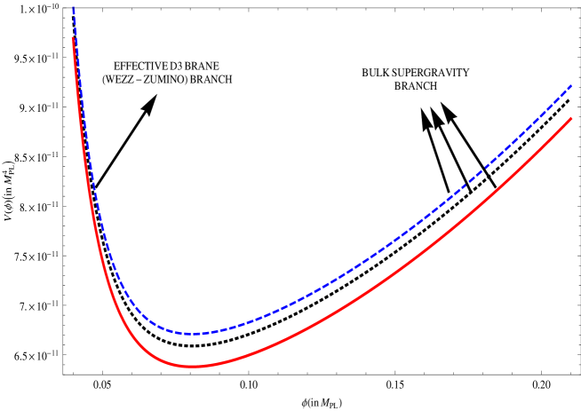
Refer to caption

Figure 1: Variation of one loop corrected potential(Vโ€‹(ฯ•)๐‘‰italic-ฯ•V(\phi)) with inflaton field (ฯ•italic-ฯ•\phi)

Figure (1) represents the inflaton potential for different values of C2โ€‹msubscript๐ถ2๐‘šC_{2m} and D2โ€‹msubscript๐ท2๐‘šD_{2m}. From the observational constraints the best fit model is given by the range: 5.67ร—10โˆ’11โ€‹MPโ€‹L4<C0<6ร—10โˆ’11โ€‹MPโ€‹L45.67superscript1011subscriptsuperscript๐‘€4๐‘ƒ๐ฟsubscript๐ถ06superscript1011subscriptsuperscript๐‘€4๐‘ƒ๐ฟ5.67\times 10^{-11}M^{4}_{PL}<C_{0}<6\times 10^{-11}M^{4}_{PL}, 1.01ร—10โˆ’16โ€‹MPโ€‹L8<Cโˆ’4<2ร—10โˆ’16โ€‹MPโ€‹L81.01superscript1016subscriptsuperscript๐‘€8๐‘ƒ๐ฟsubscript๐ถ42superscript1016subscriptsuperscript๐‘€8๐‘ƒ๐ฟ1.01\times 10^{-16}M^{8}_{PL}<C_{-4}<2\times 10^{-16}M^{8}_{PL}, 7.27ร—10โˆ’10โ€‹MPโ€‹L2<C2<7.31ร—10โˆ’10โ€‹MPโ€‹L27.27superscript1010subscriptsuperscript๐‘€2๐‘ƒ๐ฟsubscript๐ถ27.31superscript1010subscriptsuperscript๐‘€2๐‘ƒ๐ฟ7.27\times 10^{-10}M^{2}_{PL}<C_{2}<7.31\times 10^{-10}M^{2}_{PL}, 2.01ร—10โˆ’14<C4<2.45ร—10โˆ’142.01superscript1014subscript๐ถ42.45superscript10142.01\times 10^{-14}<C_{4}<2.45\times 10^{-14}, 0.014<Dโˆ’4<0.0210.014subscript๐ท40.0210.014<D_{-4}<0.021, 0.002<D2<0.0120.002subscript๐ท20.0120.002<D_{2}<0.012 and 0.011<D4<0.0190.011subscript๐ท40.0190.011<D_{4}<0.019 so that while doing numericals, we shall restrict ourselves to this range. Here MPโ€‹L=2.43ร—1018โ€‹Gโ€‹eโ€‹Vsubscript๐‘€๐‘ƒ๐ฟ2.43superscript1018๐บ๐‘’๐‘‰M_{PL}=2.43\times 10^{18}GeV represents reduced 4D Planck mass. Consequently the energy scale of inflation has a window 0.658ร—1016โ€‹Gโ€‹eโ€‹V<C04<0.667ร—1016โ€‹Gโ€‹eโ€‹V0.658superscript1016๐บ๐‘’๐‘‰4subscript๐ถ00.667superscript1016๐บ๐‘’๐‘‰0.658\times 10^{16}GeV<\sqrt[4]{C_{0}}<0.667\times 10^{16}GeV which precisely falls within the GUT scale.

Hence using equation(31) the modified Friedmann and Klein-Gordon equations can be expressed as:

H4=ฮ›(4)+8โ€‹ฯ€โ€‹G(4)โ€‹Vโ€‹(ฯ•)g~1,superscript๐ป4subscriptฮ›48๐œ‹subscript๐บ4๐‘‰italic-ฯ•subscript~๐‘”1H^{4}=\frac{\Lambda_{(4)}+8\pi G_{(4)}V(\phi)}{\tilde{g}_{1}}, (41)
ฯ•ห™2โ€‹(e2โ€‹(ฯ•)+9โ€‹e3โ€‹(ฯ•)โ€‹H2)={Vโ€ฒโ€‹(ฯ•)+C~5โ€‹g~โ€ฒโ€‹(ฯ•)โ€‹k1โˆ’D~โ€‹f~โ€ฒโ€‹(ฯ•)f~โ€‹(ฯ•)โ€‹(1โˆ’Q1)},superscriptห™italic-ฯ•2subscript๐‘’2italic-ฯ•9subscript๐‘’3italic-ฯ•superscript๐ป2superscript๐‘‰โ€ฒitalic-ฯ•subscript~๐ถ5superscript~๐‘”โ€ฒitalic-ฯ•subscript๐‘˜1~๐ทsuperscript~๐‘“โ€ฒitalic-ฯ•~๐‘“italic-ฯ•1subscript๐‘„1\dot{\phi}^{2}\left(e_{2}(\phi)+9e_{3}(\phi)H^{2}\right)=\left\{V^{{}^{\prime}}(\phi)+\tilde{C}_{5}\tilde{g}^{{}^{\prime}}(\phi)k_{1}-\frac{\tilde{D}\tilde{f}^{{}^{\prime}}(\phi)}{\tilde{f}(\phi)}\left(1-Q_{1}\right)\right\}, (42)

where e2โ€‹(ฯ•)=M~โ€‹(T,Tโ€ )โ€‹Jฯ•+2โ€‹g~โ€‹(ฯ•)โ€‹f~โ€ฒโ€‹(ฯ•)โ€‹k1โ€‹k2+8โ€‹f~โ€‹(ฯ•)โ€‹f~โ€ฒโ€‹(ฯ•)โ€‹g~โ€‹(ฯ•)โ€‹k1โ€‹k22+2โ€‹g~โ€ฒโ€‹(ฯ•)โ€‹f~โ€‹(ฯ•)โ€‹k1โ€‹k2โˆ’gโ€ฒโ€ฒโ€‹(ฯ•)โ€‹k1subscript๐‘’2italic-ฯ•~๐‘€๐‘‡superscript๐‘‡โ€ subscript๐ฝitalic-ฯ•2~๐‘”italic-ฯ•superscript~๐‘“โ€ฒitalic-ฯ•subscript๐‘˜1subscript๐‘˜28~๐‘“italic-ฯ•superscript~๐‘“โ€ฒitalic-ฯ•~๐‘”italic-ฯ•subscript๐‘˜1subscriptsuperscript๐‘˜222superscript~๐‘”โ€ฒitalic-ฯ•~๐‘“italic-ฯ•subscript๐‘˜1subscript๐‘˜2superscript๐‘”โ€ฒโ€ฒitalic-ฯ•subscript๐‘˜1e_{2}(\phi)=\tilde{M}(T,T^{{\dagger}})J_{\phi}+2\tilde{g}(\phi)\tilde{f}^{{}^{\prime}}(\phi)k_{1}k_{2}+8\tilde{f}(\phi)\tilde{f}^{{}^{\prime}}(\phi)\tilde{g}(\phi)k_{1}k^{2}_{2}+2\tilde{g}^{{}^{\prime}}(\phi)\tilde{f}(\phi)k_{1}k_{2}-g^{{}^{\prime\prime}}(\phi)k_{1} and e3โ€‹(ฯ•)=2โ€‹C~4โ€‹f~โ€‹(ฯ•)โ€‹g~โ€‹(ฯ•)โ€‹k1โ€‹k2subscript๐‘’3italic-ฯ•2subscript~๐ถ4~๐‘“italic-ฯ•~๐‘”italic-ฯ•subscript๐‘˜1subscript๐‘˜2e_{3}(\phi)=2\tilde{C}_{4}\tilde{f}(\phi)\tilde{g}(\phi)k_{1}k_{2} provided |e3โ€‹(ฯ•)|โ‰ซ|e2โ€‹(ฯ•)|much-greater-thansubscript๐‘’3italic-ฯ•subscript๐‘’2italic-ฯ•|e_{3}(\phi)|\gg|e_{2}(\phi)| in the slow-roll regime. This has been discussed in details in the Appendix B. Here we have fixed the signature of ฯ•ห™ห™italic-ฯ•\dot{\phi} so that the scalar field rolls down the potential. Additionally ghost instabilities are avoided provided the coefficient of ฯ•ห™2>0superscriptห™italic-ฯ•20\dot{\phi}^{2}>0. Consequently the potential dependent slow-roll parameters can be expressed as:

ฯตV::subscriptitalic-ฯต๐‘‰absent\displaystyle\epsilon_{V}: =\displaystyle= MPโ€‹L22โ€‹(Vโ€ฒV)2โ€‹1๐’ขโ€‹(ฯ•)โ€‹Vโ€ฒโ€‹(ฯ•),subscriptsuperscript๐‘€2๐‘ƒ๐ฟ2superscriptsuperscript๐‘‰โ€ฒ๐‘‰21๐’ขitalic-ฯ•superscript๐‘‰โ€ฒitalic-ฯ•\displaystyle\frac{M^{2}_{PL}}{2}\left(\frac{V^{{}^{\prime}}}{V}\right)^{2}\frac{1}{\sqrt{{\cal G}(\phi)V^{{}^{\prime}}(\phi)}}, (43)
ฮทV::subscript๐œ‚๐‘‰absent\displaystyle\eta_{V}: =\displaystyle= MPโ€‹L2โ€‹(Vโ€ฒโ€ฒV)โ€‹1๐’ขโ€‹(ฯ•)โ€‹Vโ€ฒโ€‹(ฯ•),subscriptsuperscript๐‘€2๐‘ƒ๐ฟsuperscript๐‘‰โ€ฒโ€ฒ๐‘‰1๐’ขitalic-ฯ•superscript๐‘‰โ€ฒitalic-ฯ•\displaystyle M^{2}_{PL}\left(\frac{V^{{}^{\prime\prime}}}{V}\right)\frac{1}{\sqrt{{\cal G}(\phi)V^{{}^{\prime}}(\phi)}}, (44)
ฮพV::subscript๐œ‰๐‘‰absent\displaystyle\xi_{V}: =\displaystyle= MPโ€‹L4โ€‹(Vโ€ฒโ€‹Vโ€ฒโ€ฒโ€ฒV2)โ€‹1๐’ขโ€‹(ฯ•)โ€‹Vโ€ฒโ€‹(ฯ•),subscriptsuperscript๐‘€4๐‘ƒ๐ฟsuperscript๐‘‰โ€ฒsuperscript๐‘‰โ€ฒโ€ฒโ€ฒsuperscript๐‘‰21๐’ขitalic-ฯ•superscript๐‘‰โ€ฒitalic-ฯ•\displaystyle M^{4}_{PL}\left(\frac{V^{{}^{\prime}}V^{{}^{\prime\prime\prime}}}{V^{2}}\right)\frac{1}{{\cal G}(\phi)V^{{}^{\prime}}(\phi)}, (45)
ฯƒV::subscript๐œŽ๐‘‰absent\displaystyle\sigma_{V}: =\displaystyle= MPโ€‹L6โ€‹((Vโ€ฒ)2โ€‹Vโ€ฒโ€ฒโ€ฒโ€ฒV3)โ€‹1(๐’ขโ€‹(ฯ•)โ€‹Vโ€ฒโ€‹(ฯ•))32,subscriptsuperscript๐‘€6๐‘ƒ๐ฟsuperscriptsuperscript๐‘‰โ€ฒ2superscript๐‘‰โ€ฒโ€ฒโ€ฒโ€ฒsuperscript๐‘‰31superscript๐’ขitalic-ฯ•superscript๐‘‰โ€ฒitalic-ฯ•32\displaystyle M^{6}_{PL}\left(\frac{(V^{{}^{\prime}})^{2}V^{{}^{\prime\prime\prime\prime}}}{V^{3}}\right)\frac{1}{\left({\cal G}(\phi)V^{{}^{\prime}}(\phi)\right)^{\frac{3}{2}}}, (46)

where ๐’ขโ€‹(ฯ•)=16โ€‹e3โ€‹(ฯ•)โ€‹MPโ€‹L2g~1โ€‹Vโ€‹(ฯ•)๐’ขitalic-ฯ•16subscript๐‘’3italic-ฯ•subscriptsuperscript๐‘€2๐‘ƒ๐ฟsubscript~๐‘”1๐‘‰italic-ฯ•{\cal G}(\phi)=\frac{16e_{3}(\phi)M^{2}_{PL}}{\tilde{g}_{1}V(\phi)}. In this connection Galileon terms effectively flatten the potential due to the presence of the flattening factor 1๐’ขโ€‹(ฯ•)โ€‹Vโ€ฒโ€‹(ฯ•)โ‰ช1much-less-than1๐’ขitalic-ฯ•superscript๐‘‰โ€ฒitalic-ฯ•1\frac{1}{\sqrt{{\cal G}(\phi)V^{{}^{\prime}}(\phi)}}\ll 1. This implies that in the presence of Galileon like derivative interaction slow-roll inflation can take place even if the potential is rather steep.

The number of e-foldings for D3 DBI Galileon can be expressed as

๐’ฉ=18โ€‹MPโ€‹Lโ€‹โˆซฯ•iฯ•f๐’ขโ€‹(ฯ•)โ€‹Vโ€ฒโ€‹(ฯ•)4ฯตVโ€‹๐‘‘ฯ•,๐’ฉ18subscript๐‘€๐‘ƒ๐ฟsubscriptsuperscriptsubscriptitalic-ฯ•๐‘“subscriptitalic-ฯ•๐‘–4๐’ขitalic-ฯ•superscript๐‘‰โ€ฒitalic-ฯ•subscriptitalic-ฯต๐‘‰differential-ditalic-ฯ•{\cal N}=\frac{1}{8M_{PL}}\int^{\phi_{f}}_{\phi_{i}}\frac{\sqrt[4]{{\cal G}(\phi)V^{{}^{\prime}}(\phi)}}{\sqrt{\epsilon_{V}}}d\phi, (47)

where ฯ•isubscriptitalic-ฯ•๐‘–\phi_{i} and ฯ•fsubscriptitalic-ฯ•๐‘“\phi_{f} are the corresponding values of the inflaton field at the beginning and end of inflation.

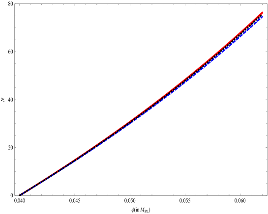
Refer to caption

Figure 2: Variation of the number of e-foldings (N๐‘N) with inflaton field (ฯ•italic-ฯ•\phi)
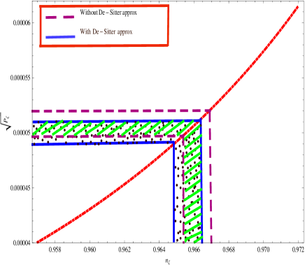
Refer to caption
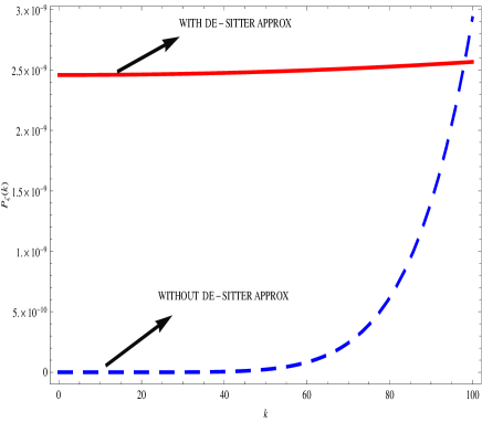
Refer to caption
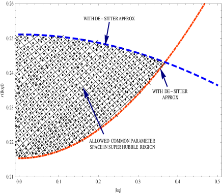
Refer to caption
Figure 3: 3Parametric plot of the amplitude of the power spectrum (๐’ซฮถsubscript๐’ซ๐œ\sqrt{{\cal P}_{\zeta}}) with scalar spectral index (nฮถsubscript๐‘›๐œn_{\zeta}), 3Variation of the scale dependent scalar power spectrum (๐’ซฮถโ€‹(k)subscript๐’ซ๐œ๐‘˜{\cal P}_{\zeta}(k)) vs momentum scale k, 3Variation of the scale dependent tensor to scalar ratio (rโ€‹(kโ€‹ฮท)๐‘Ÿ๐‘˜๐œ‚r(k\eta)) vs |kโ€‹ฮท|๐‘˜๐œ‚|k\eta| for DS and BDS analysis.

Figure(2) represents a graphical behavior of number of e-folding versus the inflaton field for different values of Ciโ€ฒโ€‹ssuperscriptsubscript๐ถ๐‘–โ€ฒ๐‘ C_{i}^{{}^{\prime}}s and the most satisfactory point in this context is the number of e-folding lies within the observational window 56<N<7056๐‘7056<N<70. The end of the inflation leads to the extra constraint Vโ€ฒโ€‹(ฯ•f)=Vโ€ฒโ€ฒโ€‹(ฯ•f)โ€‹Vโ€‹(ฯ•f)superscript๐‘‰โ€ฒsubscriptitalic-ฯ•๐‘“superscript๐‘‰โ€ฒโ€ฒsubscriptitalic-ฯ•๐‘“๐‘‰subscriptitalic-ฯ•๐‘“V^{{}^{\prime}}(\phi_{f})=\sqrt{V^{{}^{\prime\prime}}(\phi_{f})V(\phi_{f})}.

IV Quantum Fluctuations and Observable Parameters

Let us now engage ourselves in analyzing quantum fluctuation in our model and its observational imprints via primordial spectra generated from cosmological perturbation. To serve this purpose we start with the ADM formalism with the line element

dโ€‹s2=โˆ’N2โ€‹dโ€‹t2+hiโ€‹jโ€‹(Niโ€‹dโ€‹t+dโ€‹xi)โ€‹(Njโ€‹dโ€‹t+dโ€‹xj),๐‘‘superscript๐‘ 2superscript๐‘2๐‘‘superscript๐‘ก2subscriptโ„Ž๐‘–๐‘—superscript๐‘๐‘–๐‘‘๐‘ก๐‘‘superscript๐‘ฅ๐‘–superscript๐‘๐‘—๐‘‘๐‘ก๐‘‘superscript๐‘ฅ๐‘—ds^{2}=-N^{2}dt^{2}+h_{ij}(N^{i}dt+dx^{i})(N^{j}dt+dx^{j})\,, (48)

where N๐‘N and Nisuperscript๐‘๐‘–N^{i} (i=1,2,3๐‘–123i=1,2,3) are the lapse and shift functions, respectively. In this context we consider scalar metric perturbations about the flat FLRW background. Here we expand the lapse N๐‘N and the shift vector Nisuperscript๐‘๐‘–N^{i}, as N=1+ฮฑ๐‘1๐›ผN=1+\alpha and Ni=โˆ‚iฯˆ+N~isubscript๐‘๐‘–subscript๐‘–๐œ“subscript~๐‘๐‘–N_{i}=\partial_{i}\psi+\tilde{N}_{i}, respectively. Here โˆ‚iฯˆsubscript๐‘–๐œ“\partial_{i}\psi is the irrotational part and N~isubscript~๐‘๐‘–\tilde{N}_{i} be the incomressible vector part (N~i,i=โˆ‚iN~i=0subscript~๐‘๐‘–๐‘–subscript๐‘–subscript~๐‘๐‘–0\tilde{N}_{i,i}=\partial_{i}\tilde{N}_{i}=0). These are actually non-dynamical Lagrange multipliers in the action, so that it is sufficient to know N๐‘N and Nisuperscript๐‘๐‘–N^{i} up to first order. This implies their equation of motion is purely algebraic. To fix the time and spatial reparameterizaion we choose the uniform-field gauge with ฮดโ€‹ฯ•=0๐›ฟitalic-ฯ•0\delta\phi=0, which fixes the temporal component of a gauge-transformation vector ฮพฮผsuperscript๐œ‰๐œ‡\xi^{\mu}. After that by fixing the spatial part of ฮพฮผsuperscript๐œ‰๐œ‡\xi^{\mu} we gauge away a field ฮต๐œ€\varepsilon that appears as a form ฮต,ij\varepsilon_{,ij} inside hiโ€‹jsubscriptโ„Ž๐‘–๐‘—h_{ij}. Consequently the metric on three dimensional constant time slice can be expressed as hiโ€‹j=a2โ€‹(t)โ€‹e2โ€‹ฮถโ€‹ฮดiโ€‹jsubscriptโ„Ž๐‘–๐‘—superscript๐‘Ž2๐‘กsuperscript๐‘’2๐œsubscript๐›ฟ๐‘–๐‘—h_{ij}=a^{2}(t)e^{2{\zeta}}\delta_{ij}. Plugging all of these informations in to equation(48) we get:

ds2=โˆ’[(1+ฮฑ)2โˆ’aโˆ’2(t)eโˆ’2โ€‹ฮถ{(โˆ‚ฯˆ)2+N~2+2N~.(โˆ‚ฯˆ)}]dt2+2[โˆ‚iฯˆ+N~i]dtdxi+a2(t)e2โ€‹ฮถฮดiโ€‹jdxidxj,ds^{2}=-\left[(1+\alpha)^{2}-a^{-2}(t)e^{-2{\zeta}}\left\{(\partial\psi)^{2}+\tilde{N}^{2}+2\tilde{N}.(\partial\psi)\right\}\right]\,dt^{2}+2\left[\partial_{i}\psi+\tilde{N}_{i}\right]\,dt\,dx^{i}+a^{2}(t)e^{2{\zeta}}\delta_{ij}dx^{i}dx^{j}, (49)

where we use a shorthand notation (โˆ‚ฯˆ)2=(โˆ‚ฯˆi)โ€‹(โˆ‚ฯˆi)โ‰ก(โˆ‚iฯˆ)โ€‹(โˆ‚iฯˆ)superscript๐œ“2subscript๐œ“๐‘–subscript๐œ“๐‘–subscript๐‘–๐œ“subscript๐‘–๐œ“(\partial\psi)^{2}=(\partial\psi_{i})\,(\partial\psi_{i})\equiv(\partial_{i}\psi)(\partial_{i}\psi). At linear level of the perturbation theory equation(49) reuces to the following metric:

dโ€‹s2=โˆ’(1+2โ€‹ฮฑ)โ€‹dโ€‹t2+2โ€‹[โˆ‚iฯˆ+N~i]โ€‹dโ€‹tโ€‹dโ€‹xi+a2โ€‹(t)โ€‹(1+2โ€‹ฮถ)โ€‹ฮดiโ€‹jโ€‹dโ€‹xiโ€‹dโ€‹xj.๐‘‘superscript๐‘ 212๐›ผ๐‘‘superscript๐‘ก22delimited-[]subscript๐‘–๐œ“subscript~๐‘๐‘–๐‘‘๐‘ก๐‘‘superscript๐‘ฅ๐‘–superscript๐‘Ž2๐‘ก12๐œsubscript๐›ฟ๐‘–๐‘—๐‘‘superscript๐‘ฅ๐‘–๐‘‘superscript๐‘ฅ๐‘—ds^{2}=-(1+2\alpha)\,dt^{2}+2\left[\partial_{i}\psi+\tilde{N}_{i}\right]\,dt\,dx^{i}+a^{2}(t)\,(1+2\zeta)\,\delta_{ij}dx^{i}dx^{j}\,. (50)

Expanding the four dimensional effective action stated in equation(33) up to second order, we get:

S2ฮถ=โˆซ๐‘‘tโ€‹d3โ€‹xโ€‹a3โ€‹[โˆ’3โ€‹t1โ€‹ฮถห™2+2โ€‹w1a2โ€‹ฮถห™โ€‹โˆ‚2ฯˆโˆ’t2a2โ€‹ฮฑโ€‹โˆ‚2ฯˆโˆ’2โ€‹t1a2โ€‹ฮฑโ€‹โˆ‚2ฮถ+3โ€‹t2โ€‹ฮฑโ€‹ฮถห™+13โ€‹t3โ€‹ฮฑ2+t4a2โ€‹โˆ‚iฮถโ€‹โˆ‚iฮถ],subscriptsuperscript๐‘†๐œ2differential-d๐‘กsuperscript๐‘‘3๐‘ฅsuperscript๐‘Ž3delimited-[]3subscript๐‘ก1superscriptห™๐œ22subscript๐‘ค1superscript๐‘Ž2ห™๐œsuperscript2๐œ“subscript๐‘ก2superscript๐‘Ž2๐›ผsuperscript2๐œ“2subscript๐‘ก1superscript๐‘Ž2๐›ผsuperscript2๐œ3subscript๐‘ก2๐›ผห™๐œ13subscript๐‘ก3superscript๐›ผ2subscript๐‘ก4superscript๐‘Ž2subscript๐‘–๐œsubscript๐‘–๐œS^{\zeta}_{2}=\int dt\,d^{3}x\,a^{3}\left[-3t_{1}\dot{\zeta}^{2}+\frac{2w_{1}}{a^{2}}\dot{\zeta}\partial^{2}\psi-\frac{t_{2}}{a^{2}}\alpha\partial^{2}\psi-\frac{2t_{1}}{a^{2}}\alpha\partial^{2}{\zeta}+3t_{2}\,\alpha\,\dot{\zeta}+\frac{1}{3}t_{3}\alpha^{2}+\frac{t_{4}}{a^{2}}\,\partial_{i}{\zeta}\,\partial_{i}{\zeta}\right]\,, (51)

where the effect of effective Gauss-Bonnet coupling and the DBI Galileon features are explicitly appearing in the co-efficients of the second order perturbative action as:

t1subscript๐‘ก1\displaystyle t_{1} โ‰ˆ\displaystyle\approx l~1,subscript~๐‘™1\displaystyle\tilde{l}_{1}\,, (52)
t2subscript๐‘ก2\displaystyle t_{2} โ‰ˆ\displaystyle\approx (2โ€‹Hโ€‹l~1โˆ’2โ€‹ฯ•ห™โ€‹Xโ€‹G~X),2๐ปsubscript~๐‘™12ห™italic-ฯ•๐‘‹subscript~๐บ๐‘‹\displaystyle\left(2H\tilde{l}_{1}-2\dot{\phi}X\tilde{G}_{X}\right)\,, (53)
t3subscript๐‘ก3\displaystyle t_{3} โ‰ˆ\displaystyle\approx โˆ’9โ€‹l~1โ€‹H2+3โ€‹(Xโ€‹K~^X+2โ€‹X2โ€‹K~^Xโ€‹X)9subscript~๐‘™1superscript๐ป23๐‘‹subscript^~๐พ๐‘‹2superscript๐‘‹2subscript^~๐พ๐‘‹๐‘‹\displaystyle-9\tilde{l}_{1}H^{2}+3\left(X\hat{\tilde{K}}_{X}+2X^{2}\hat{\tilde{K}}_{XX}\right) (54)
+18โ€‹Hโ€‹ฯ•ห™โ€‹(2โ€‹Xโ€‹G~X+X2โ€‹G~Xโ€‹X)โˆ’6โ€‹(Xโ€‹G,ฯ•+X2โ€‹G,ฯ•X),\displaystyle{}+18H\dot{\phi}\left(2X\tilde{G}_{X}+X^{2}\tilde{G}_{XX}\right)-6(XG_{,\phi}+X^{2}G_{,\phi X})\,,
t4subscript๐‘ก4\displaystyle t_{4} โ‰ˆ\displaystyle\approx l~1.subscript~๐‘™1\displaystyle\tilde{l}_{1}\,. (55)

It is important to mention here that, in the action (51), both the coefficients of the terms ฮฑโ€‹ฮถ๐›ผ๐œ\alpha{\zeta} and ฮถ2superscript๐œ2{\zeta}^{2} vanish by using the background equations of motion. Furthermore, in (51), the term quadratic in ฯˆ๐œ“\psi vanishes by making use of integrations by parts. The equations of motion for ฯˆ๐œ“\psi and ฮฑ๐›ผ\alpha, derived from (51), lead to the following two-fold constraint relations:

ฮฑ๐›ผ\displaystyle\alpha =\displaystyle= ๐’ฅโ€‹ฮถห™,๐’ฅห™๐œ\displaystyle{\cal J}\dot{{\zeta}}\,, (56)
1a2โ€‹โˆ‚2ฯˆ1superscript๐‘Ž2superscript2๐œ“\displaystyle\frac{1}{a^{2}}\,\partial^{2}\psi =\displaystyle= 2โ€‹t33โ€‹t2โ€‹ฮฑ+3โ€‹ฮถห™โˆ’2โ€‹t1t2โ€‹1a2โ€‹โˆ‚2ฮถ,2subscript๐‘ก33subscript๐‘ก2๐›ผ3ห™๐œ2subscript๐‘ก1subscript๐‘ก21superscript๐‘Ž2superscript2๐œ\displaystyle\frac{2t_{3}}{3t_{2}}\,\alpha+3\dot{\zeta}-\frac{2t_{1}}{t_{2}}\frac{1}{a^{2}}\partial^{2}{\zeta}\,, (57)

where

๐’ฅโ‰ก2โ€‹t1t2=2โ€‹l~1(2โ€‹Hโ€‹l~1โˆ’2โ€‹ฯ•ห™โ€‹Xโ€‹G~X).๐’ฅ2subscript๐‘ก1subscript๐‘ก22subscript~๐‘™12๐ปsubscript~๐‘™12ห™italic-ฯ•๐‘‹subscript~๐บ๐‘‹{\cal J}\equiv\frac{2t_{1}}{t_{2}}=\frac{2\tilde{l}_{1}}{\left(2H\tilde{l}_{1}-2\dot{\phi}X\tilde{G}_{X}\right)}\,. (58)

Using expansion in terms of the slow-parameter defined in equationย (75) gives

๐’ฅ=1Hโ€‹[1+ฮดGโ€‹X+๐’ชโ€‹(ฯตV2)].๐’ฅ1๐ปdelimited-[]1subscript๐›ฟ๐บ๐‘‹๐’ชsubscriptsuperscriptitalic-ฯต2๐‘‰{\cal J}=\frac{1}{H}\left[1+\delta_{GX}+{\cal O}(\epsilon^{2}_{V})\right]\,. (59)

Then substituting equation(56) and equation(57) into equationย (51) and integrating the term ฮถห™โ€‹โˆ‚2ฮถห™๐œsuperscript2๐œ\dot{\zeta}\partial^{2}{\zeta} by parts the second order action stated in equation(51) can be re-expressed as:

S2ฮถ=โˆซ๐‘‘tโ€‹d3โ€‹xโ€‹a3โ€‹YSโ€‹[ฮถห™2โˆ’cs2a2โ€‹(โˆ‚ฮถ)2],subscriptsuperscript๐‘†๐œ2differential-d๐‘กsuperscript๐‘‘3๐‘ฅsuperscript๐‘Ž3subscript๐‘Œ๐‘†delimited-[]superscriptห™๐œ2subscriptsuperscript๐‘2๐‘ superscript๐‘Ž2superscript๐œ2S^{\zeta}_{2}=\int dtd^{3}xa^{3}Y_{S}\left[\dot{\zeta}^{2}-\frac{c^{2}_{s}}{a^{2}}(\partial\zeta)^{2}\right], (60)

where

YSsubscript๐‘Œ๐‘†\displaystyle Y_{S} =\displaystyle= t1โ€‹(4โ€‹t1โ€‹t3+9โ€‹t22)3โ€‹t22,subscript๐‘ก14subscript๐‘ก1subscript๐‘ก39subscriptsuperscript๐‘ก223subscriptsuperscript๐‘ก22\displaystyle\frac{t_{1}\left(4t_{1}t_{3}+9t^{2}_{2}\right)}{3t^{2}_{2}}, (61)
cs2subscriptsuperscript๐‘2๐‘ \displaystyle c^{2}_{s} =\displaystyle= 3โ€‹(2โ€‹Hโ€‹t2โ€‹t12โˆ’t4โ€‹t22โˆ’2โ€‹t12โ€‹tห™2)t1โ€‹(4โ€‹t1โ€‹t3+9โ€‹t22).32๐ปsubscript๐‘ก2subscriptsuperscript๐‘ก21subscript๐‘ก4subscriptsuperscript๐‘ก222subscriptsuperscript๐‘ก21subscriptห™๐‘ก2subscript๐‘ก14subscript๐‘ก1subscript๐‘ก39subscriptsuperscript๐‘ก22\displaystyle\frac{3\left(2Ht_{2}t^{2}_{1}-t_{4}t^{2}_{2}-2t^{2}_{1}\dot{t}_{2}\right)}{t_{1}\left(4t_{1}t_{3}+9t^{2}_{2}\right)}. (62)

It is important to mention here that ghosts and Laplacian instabilities can be avoided iff cs2>0,YS>0formulae-sequencesubscriptsuperscript๐‘2๐‘ 0subscript๐‘Œ๐‘†0c^{2}_{s}>0,Y_{S}>0. Now using equation(56) and equation(61) in equation(57) we get:

ฯˆ๐œ“\displaystyle\psi =\displaystyle= โˆ’๐’ฅโ€‹ฮถ+โˆ‚โˆ’2(a2โ€‹YSโ€‹ฮถห™t1).๐’ฅ๐œsuperscript2superscript๐‘Ž2subscript๐‘Œ๐‘†ห™๐œsubscript๐‘ก1\displaystyle-{\cal J}\zeta+\partial^{-2}\left(\frac{a^{2}Y_{S}\dot{\zeta}}{t_{1}}\right). (63)

For future convenience, we have introduced a new parameter defined as:

ฯตs=YSโ€‹cs2l~1=(2โ€‹Hโ€‹t2โ€‹t12โˆ’t4โ€‹t22โˆ’2โ€‹t12โ€‹tห™2)t22โ€‹l~1=ฯตV+ฮดGโ€‹X+๐’ชโ€‹(ฯตV2)subscriptitalic-ฯต๐‘ subscript๐‘Œ๐‘†subscriptsuperscript๐‘2๐‘ subscript~๐‘™12๐ปsubscript๐‘ก2subscriptsuperscript๐‘ก21subscript๐‘ก4subscriptsuperscript๐‘ก222subscriptsuperscript๐‘ก21subscriptห™๐‘ก2subscriptsuperscript๐‘ก22subscript~๐‘™1subscriptitalic-ฯต๐‘‰subscript๐›ฟ๐บ๐‘‹๐’ชsubscriptsuperscriptitalic-ฯต2๐‘‰missing-subexpressionmissing-subexpression\begin{array}[]{lll}\displaystyle\epsilon_{s}=\frac{Y_{S}c^{2}_{s}}{\tilde{l}_{1}}=\frac{\left(2Ht_{2}t^{2}_{1}-t_{4}t^{2}_{2}-2t^{2}_{1}\dot{t}_{2}\right)}{t^{2}_{2}\tilde{l}_{1}}=\epsilon_{V}+\delta_{GX}+{\cal O}(\epsilon^{2}_{V})\end{array} (64)

where we use equationย (43) and equationย (75) to express it in terms of slow-roll parameters. Now varying the action stated in equation(60) and expressing the solution at the linear level in terms of Fourier modes, we arrive at the Mukhanov Sasaki Equation for Galileon scalar mode.

vkโ†’โ€ฒโ€ฒ+(cs2โ€‹k2โˆ’zโ€ฒโ€ฒz)โ€‹vkโ†’=0,subscriptsuperscript๐‘ฃโ€ฒโ€ฒโ†’๐‘˜subscriptsuperscript๐‘2๐‘ superscript๐‘˜2superscript๐‘งโ€ฒโ€ฒ๐‘งsubscript๐‘ฃโ†’๐‘˜0v^{{}^{\prime\prime}}_{\vec{k}}+\left(c^{2}_{s}k^{2}-\frac{z^{{}^{\prime\prime}}}{z}\right)v_{\vec{k}}=0, (65)

where cs2subscriptsuperscript๐‘2๐‘ c^{2}_{s} takes into account the nontrivial modification due to Galileon. Similarly for tensor modes, equation(60) can be recast as:

S2h=โˆซ๐‘‘tโ€‹d3โ€‹xโ€‹a3โ€‹YTโ€‹[hห™iโ€‹j2โˆ’cs2a2โ€‹(โˆ‚hiโ€‹j)2],subscriptsuperscript๐‘†โ„Ž2differential-d๐‘กsuperscript๐‘‘3๐‘ฅsuperscript๐‘Ž3subscript๐‘Œ๐‘‡delimited-[]subscriptsuperscriptห™โ„Ž2๐‘–๐‘—subscriptsuperscript๐‘2๐‘ superscript๐‘Ž2superscriptsubscriptโ„Ž๐‘–๐‘—2S^{h}_{2}=\int dtd^{3}xa^{3}Y_{T}\left[\dot{h}^{2}_{ij}-\frac{c^{2}_{s}}{a^{2}}(\partial h_{ij})^{2}\right], (66)

where

YTsubscript๐‘Œ๐‘‡\displaystyle Y_{T} =\displaystyle= t14=l~14,subscript๐‘ก14subscript~๐‘™14\displaystyle\frac{t_{1}}{4}=\frac{\tilde{l}_{1}}{4}, (67)
cT2subscriptsuperscript๐‘2๐‘‡\displaystyle c^{2}_{T} =\displaystyle= t4t1=1+๐’ชโ€‹(ฯต2).subscript๐‘ก4subscript๐‘ก11๐’ชsuperscriptitalic-ฯต2\displaystyle\frac{t_{4}}{t_{1}}=1+{\cal O}(\epsilon^{2}). (68)

For tensor modes we use the normalization condition eiโ€‹jฮปโ€‹eiโ€‹jฮปโ€ฒ=2โ€‹ฮดฮปโ€‹ฮปโ€ฒsubscriptsuperscript๐‘’๐œ†๐‘–๐‘—subscriptsuperscript๐‘’superscript๐œ†โ€ฒ๐‘–๐‘—2superscript๐›ฟ๐œ†superscript๐œ†โ€ฒe^{\lambda}_{ij}e^{\lambda^{{}^{\prime}}}_{ij}=2\delta^{\lambda\lambda^{{}^{\prime}}} and traceless condition eiโ€‹i=0subscript๐‘’๐‘–๐‘–0e_{ii}=0 for polarization tensor. Following the same prescription we can establish equation(65) for tensor modes provided cssubscript๐‘๐‘ c_{s} is replaced by cTsubscript๐‘๐‘‡c_{T}. The Bunch-Davies mode function turns out to be (Throughout the paper we have used DS for de-Sitter results and BDS for beyond de-Sitter results.)

uฮถโ€‹(ฮท,k)={iโ€‹Hโ€‹expโก(โˆ’iโ€‹kโ€‹csโ€‹ฮท)2โ€‹YSโ€‹(csโ€‹k)32โ€‹(1+iโ€‹kโ€‹csโ€‹ฮท)ย :DSโˆ’kโ€‹ฮทโ€‹csaโ€‹2โ€‹YSโ€‹โ„‹ฮฝs(1)โ€‹(โˆ’kโ€‹ฮทโ€‹cs)ย :BDSย .subscript๐‘ข๐œ๐œ‚๐‘˜cases๐‘–๐ป๐‘–๐‘˜subscript๐‘๐‘ ๐œ‚2subscript๐‘Œ๐‘†superscriptsubscript๐‘๐‘ ๐‘˜321๐‘–๐‘˜subscript๐‘๐‘ ๐œ‚ย :DS๐‘˜๐œ‚subscript๐‘๐‘ ๐‘Ž2subscript๐‘Œ๐‘†subscriptsuperscriptโ„‹1subscript๐œˆ๐‘ ๐‘˜๐œ‚subscript๐‘๐‘ ย :BDSย u_{\zeta}(\eta,k)=\left\{\begin{array}[]{ll}\displaystyle\frac{iH\exp(-ikc_{s}\eta)}{2\sqrt{Y_{S}}(c_{s}k)^{\frac{3}{2}}}\left(1+ikc_{s}\eta\right)&\mbox{~{}~{}~{}~{} \it:{\cal DS}}\\ \displaystyle\frac{\sqrt{-k\eta c_{s}}}{a\sqrt{2Y_{S}}}{\cal H}^{(1)}_{\nu_{s}}(-k\eta c_{s})&\mbox{~{}~{}~{}~{}~{}\it:{\cal BDS }}.\end{array}\right. (69)

where ฮฝs=(3โˆ’ฯตVโˆ’2โ€‹sVS+ฮดV2โ€‹(1โˆ’ฯตVโˆ’sVS))subscript๐œˆ๐‘ 3subscriptitalic-ฯต๐‘‰2subscriptsuperscript๐‘ ๐‘†๐‘‰subscript๐›ฟ๐‘‰21subscriptitalic-ฯต๐‘‰subscriptsuperscript๐‘ ๐‘†๐‘‰\nu_{s}=\left(\frac{3-\epsilon_{V}-2s^{S}_{V}+\delta_{V}}{2(1-\epsilon_{V}-s^{S}_{V})}\right) and in the super-Hubble limit we have:

โ„‹ฮฝs(1)subscriptsuperscriptโ„‹1subscript๐œˆ๐‘ \displaystyle{\cal H}^{(1)}_{\nu_{s}} โ†’โ†’\displaystyle\rightarrow (โˆ’kโ€‹csโ€‹ฮท)โˆ’ฮฝsโ€‹expโก(iโ€‹[ฮฝsโˆ’12]โ€‹ฯ€2)โ€‹2ฮฝsโˆ’322โ€‹csโ€‹kโ€‹(ฮ“โ€‹(ฮฝs)ฮ“โ€‹(32))superscript๐‘˜subscript๐‘๐‘ ๐œ‚subscript๐œˆ๐‘ ๐‘–delimited-[]subscript๐œˆ๐‘ 12๐œ‹2superscript2subscript๐œˆ๐‘ 322subscript๐‘๐‘ ๐‘˜ฮ“subscript๐œˆ๐‘ ฮ“32\displaystyle\frac{\left(-kc_{s}\eta\right)^{-\nu_{s}}\exp\left(i[\nu_{s}-\frac{1}{2}]\frac{\pi}{2}\right)2^{\nu_{s}-\frac{3}{2}}}{\sqrt{2c_{s}k}}\left(\frac{\Gamma(\nu_{s})}{\Gamma(\frac{3}{2})}\right) (70)

. Further we have introduced five new parameters during the analysis of primordial quantum fluctuation defined as:

sVS::subscriptsuperscript๐‘ ๐‘†๐‘‰absent\displaystyle s^{S}_{V}: =\displaystyle= csห™Hโ€‹cs=4โ€‹Vโ€ฒโ€‹(ฯ•)โ€‹MPโ€‹L2๐’ขโ€‹(ฯ•)โ€‹ddโ€‹ฯ•โ€‹(lnโกcs),ห™subscript๐‘๐‘ ๐ปsubscript๐‘๐‘ 4superscript๐‘‰โ€ฒitalic-ฯ•subscriptsuperscript๐‘€2๐‘ƒ๐ฟ๐’ขitalic-ฯ•๐‘‘๐‘‘italic-ฯ•subscript๐‘๐‘ \displaystyle\frac{\dot{c_{s}}}{Hc_{s}}=\frac{4\sqrt{V^{{}^{\prime}}(\phi)}M^{2}_{PL}}{\sqrt{{\cal G}(\phi)}}\frac{d}{d\phi}\left(\ln c_{s}\right), (71)
sVT::subscriptsuperscript๐‘ ๐‘‡๐‘‰absent\displaystyle s^{T}_{V}: =\displaystyle= cTห™Hโ€‹cT=MPโ€‹Lโ€‹g~1โ€‹Vโ€ฒโ€‹(ฯ•)2โ€‹e3โ€‹(ฯ•)โ€‹Vโ€‹(ฯ•)โ€‹ddโ€‹ฯ•โ€‹(lnโก[1+๐’ชโ€‹(ฯตV2)]),ห™subscript๐‘๐‘‡๐ปsubscript๐‘๐‘‡subscript๐‘€๐‘ƒ๐ฟsubscript~๐‘”1superscript๐‘‰โ€ฒitalic-ฯ•2subscript๐‘’3italic-ฯ•๐‘‰italic-ฯ•๐‘‘๐‘‘italic-ฯ•1๐’ชsubscriptsuperscriptitalic-ฯต2๐‘‰\displaystyle\frac{\dot{c_{T}}}{Hc_{T}}=\frac{M_{PL}\sqrt{\tilde{g}_{1}V^{{}^{\prime}}(\phi)}}{2\sqrt{e_{3}(\phi)V(\phi)}}\frac{d}{d\phi}\left(\ln\left[1+{\cal O}(\epsilon^{2}_{V})\right]\right), (72)
ฮทs::subscript๐œ‚๐‘ absent\displaystyle\eta_{s}: =\displaystyle= ฯตsห™Hโ€‹ฯตs=4โ€‹Vโ€ฒโ€‹(ฯ•)โ€‹MPโ€‹L2๐’ขโ€‹(ฯ•)โ€‹[ฯตVโ€ฒโ€‹(1+๐’ชโ€‹(ฯตV))+ฮดGโ€‹Xโ€‹ฯ•][ฯตV+ฮดGโ€‹X+๐’ชโ€‹(ฯตV2)],ห™subscriptitalic-ฯต๐‘ ๐ปsubscriptitalic-ฯต๐‘ 4superscript๐‘‰โ€ฒitalic-ฯ•subscriptsuperscript๐‘€2๐‘ƒ๐ฟ๐’ขitalic-ฯ•delimited-[]subscriptsuperscriptitalic-ฯตโ€ฒ๐‘‰1๐’ชsubscriptitalic-ฯต๐‘‰subscript๐›ฟ๐บ๐‘‹italic-ฯ•delimited-[]subscriptitalic-ฯต๐‘‰subscript๐›ฟ๐บ๐‘‹๐’ชsubscriptsuperscriptitalic-ฯต2๐‘‰\displaystyle\frac{\dot{\epsilon_{s}}}{H\epsilon_{s}}=\frac{4\sqrt{V^{{}^{\prime}}(\phi)}M^{2}_{PL}}{\sqrt{{\cal G}(\phi)}}\frac{\left[\epsilon^{{}^{\prime}}_{V}\left(1+{\cal O}(\epsilon_{V})\right)+\delta_{GX\phi}\right]}{\left[\epsilon_{V}+\delta_{GX}+{\cal O}(\epsilon^{2}_{V})\right]}, (73)
ฮดV::subscript๐›ฟ๐‘‰absent\displaystyle\delta_{V}: =\displaystyle= Ysห™Hโ€‹Ys=4โ€‹Vโ€ฒโ€‹(ฯ•)โ€‹MPโ€‹L2๐’ขโ€‹(ฯ•)โ€‹ddโ€‹ฯ•โ€‹(lnโกYs),ห™subscript๐‘Œ๐‘ ๐ปsubscript๐‘Œ๐‘ 4superscript๐‘‰โ€ฒitalic-ฯ•subscriptsuperscript๐‘€2๐‘ƒ๐ฟ๐’ขitalic-ฯ•๐‘‘๐‘‘italic-ฯ•subscript๐‘Œ๐‘ \displaystyle\frac{\dot{Y_{s}}}{HY_{s}}=\frac{4\sqrt{V^{{}^{\prime}}(\phi)}M^{2}_{PL}}{\sqrt{{\cal G}(\phi)}}\frac{d}{d\phi}\left(\ln Y_{s}\right), (74)
ฮดGโ€‹X::subscript๐›ฟ๐บ๐‘‹absent\displaystyle\delta_{GX}: =\displaystyle= ฯ•ห™โ€‹Xโ€‹G~Xl~1.ห™italic-ฯ•๐‘‹subscript~๐บ๐‘‹subscript~๐‘™1\displaystyle\frac{\dot{\phi}X\tilde{G}_{X}}{\tilde{l}_{1}}. (75)

Now using eqn(69) the two-point correlation function for scalar modes can be expressed as:

โŸจ0|ฮถโ€‹(kโ†’)โ€‹ฮถโ€‹(kโ€ฒโ†’)|0โŸฉ=2โ€‹ฯ€2k3โ€‹(2โ€‹ฯ€)3โ€‹๐’ซฮถโ€‹(k)โ€‹ฮด3โ€‹(kโ†’+kโ€ฒโ†’)=(2โ€‹ฯ€)3โ€‹|uฮถโ€‹(ฮท,k)|2โ€‹ฮด3โ€‹(kโ†’+kโ€ฒโ†’),quantum-operator-product0๐œโ†’๐‘˜๐œโ†’superscript๐‘˜โ€ฒ02superscript๐œ‹2superscript๐‘˜3superscript2๐œ‹3subscript๐’ซ๐œ๐‘˜superscript๐›ฟ3โ†’๐‘˜โ†’superscript๐‘˜โ€ฒsuperscript2๐œ‹3superscriptsubscript๐‘ข๐œ๐œ‚๐‘˜2superscript๐›ฟ3โ†’๐‘˜โ†’superscript๐‘˜โ€ฒ\langle 0|\zeta(\vec{k})\zeta(\vec{k^{{}^{\prime}}})|0\rangle=\frac{2\pi^{2}}{k^{3}}(2\pi)^{3}{\cal P}_{\zeta}(k)\delta^{3}(\vec{k}+\vec{k^{{}^{\prime}}})=(2\pi)^{3}|u_{\zeta}(\eta,k)|^{2}\delta^{3}(\vec{k}+\vec{k^{{}^{\prime}}}), (76)

where the dimensionless Power spectrum for scalar modes ๐’ซฮถโ€‹(k)subscript๐’ซ๐œ๐‘˜{\cal P}_{\zeta}(k) at the horizon crossing turns out to be:

๐’ซฮถโ€‹(kโ‹†)=kโ‹†32โ€‹ฯ€2โ€‹|uฮถโ€‹(kโ‹†)|2={(Vโ€‹(ฯ•)8โ€‹ฯ€2โ€‹csโ€‹ฯตsโ€‹l~1โ€‹g~1โ€‹MPโ€‹L)โ‹†ย :DS(22โ€‹ฮฝsโˆ’3โ€‹|ฮ“โ€‹(ฮฝs)ฮ“โ€‹(32)|2โ€‹(1โˆ’ฯตVโˆ’sVS)2โ€‹Vโ€‹(ฯ•)8โ€‹ฯ€2โ€‹YSโ€‹cs3โ€‹g~1โ€‹MPโ€‹L)โ‹†ย :BDSย .subscript๐’ซ๐œsubscript๐‘˜โ‹†subscriptsuperscript๐‘˜3โ‹†2superscript๐œ‹2superscriptsubscript๐‘ข๐œsubscript๐‘˜โ‹†2casessubscript๐‘‰italic-ฯ•8superscript๐œ‹2subscript๐‘๐‘ subscriptitalic-ฯต๐‘ subscript~๐‘™1subscript~๐‘”1subscript๐‘€๐‘ƒ๐ฟโ‹†ย :DSsubscriptsuperscript22subscript๐œˆ๐‘ 3superscriptฮ“subscript๐œˆ๐‘ ฮ“322superscript1subscriptitalic-ฯต๐‘‰subscriptsuperscript๐‘ ๐‘†๐‘‰2๐‘‰italic-ฯ•8superscript๐œ‹2subscript๐‘Œ๐‘†subscriptsuperscript๐‘3๐‘ subscript~๐‘”1subscript๐‘€๐‘ƒ๐ฟโ‹†ย :BDSย {\cal P}_{\zeta}(k_{\star})=\frac{k^{3}_{\star}}{2\pi^{2}}|u_{\zeta}(k_{\star})|^{2}=\left\{\begin{array}[]{ll}\displaystyle\left(\frac{\sqrt{V(\phi)}}{8\pi^{2}c_{s}\epsilon_{s}\tilde{l}_{1}\sqrt{\tilde{g}_{1}}M_{PL}}\right)_{\star}&\mbox{~{} \it:{\cal DS}}\\ \displaystyle\left(2^{2\nu_{s}-3}\left|\frac{\Gamma(\nu_{s})}{\Gamma(\frac{3}{2})}\right|^{2}\frac{\left(1-\epsilon_{V}-s^{S}_{V}\right)^{2}\sqrt{V(\phi)}}{8\pi^{2}Y_{S}c^{3}_{s}\sqrt{\tilde{g}_{1}}M_{PL}}\right)_{\star}&\mbox{~{}~{}\it:{\cal BDS }}.\end{array}\right. (77)

โ‹†โ‹†\star corresponds to the horizon crossing. Similarly using the tensor version of eqn(69) the two-point correlation function for tensor modes can be expressed as:

โŸจ0|hiโ€‹jโ€‹(kโ†’)โ€‹hiโ€‹jโ€‹(kโ€ฒโ†’)|0โŸฉ=2โ€‹ฯ€2k3โ€‹(2โ€‹ฯ€)3โ€‹๐’ซTโ€‹(k)โ€‹ฮด3โ€‹(kโ†’+kโ€ฒโ†’)=(2โ€‹ฯ€)3โ€‹|uฮถโ€‹(ฮท,k)|2โ€‹ฮด3โ€‹(kโ†’+kโ€ฒโ†’),quantum-operator-product0subscriptโ„Ž๐‘–๐‘—โ†’๐‘˜subscriptโ„Ž๐‘–๐‘—โ†’superscript๐‘˜โ€ฒ02superscript๐œ‹2superscript๐‘˜3superscript2๐œ‹3subscript๐’ซ๐‘‡๐‘˜superscript๐›ฟ3โ†’๐‘˜โ†’superscript๐‘˜โ€ฒsuperscript2๐œ‹3superscriptsubscript๐‘ข๐œ๐œ‚๐‘˜2superscript๐›ฟ3โ†’๐‘˜โ†’superscript๐‘˜โ€ฒ\langle 0|h_{ij}(\vec{k})h_{ij}(\vec{k^{{}^{\prime}}})|0\rangle=\frac{2\pi^{2}}{k^{3}}(2\pi)^{3}{\cal P}_{T}(k)\delta^{3}(\vec{k}+\vec{k^{{}^{\prime}}})=(2\pi)^{3}|u_{\zeta}(\eta,k)|^{2}\delta^{3}(\vec{k}+\vec{k^{{}^{\prime}}}), (78)

where ๐’ซTโ€‹(k)=[๐’ซTโ€‹(k)]iโ€‹j;iโ€‹jsubscript๐’ซ๐‘‡๐‘˜subscriptdelimited-[]subscript๐’ซ๐‘‡๐‘˜๐‘–๐‘—๐‘–๐‘—{\cal P}_{T}(k)=[{\cal P}_{T}(k)]_{ij;ij} and the corresponding dimensionless Power spectrum for tensor modes reads:

๐’ซTโ€‹(kโ‹†)=kโ‹†32โ€‹ฯ€2โ€‹|uhโ€‹(kโ‹†)|2โ€‹(โˆ‘ฮป=+,ร—eiโ€‹jฮปโ€‹eiโ€‹jฮป)={(Vโ€‹(ฯ•)2โ€‹ฯ€2โ€‹cTโ€‹ฯตTโ€‹l~1โ€‹g~1โ€‹MPโ€‹L)โ‹†ย :DS(22โ€‹ฮฝTโˆ’3โ€‹|ฮ“โ€‹(ฮฝT)ฮ“โ€‹(32)|2โ€‹(1โˆ’ฯตVโˆ’sVT)2โ€‹Vโ€‹(ฯ•)2โ€‹ฯ€2โ€‹YTโ€‹cT3โ€‹g~1โ€‹MPโ€‹L)โ‹†ย :BDSย .subscript๐’ซ๐‘‡subscript๐‘˜โ‹†subscriptsuperscript๐‘˜3โ‹†2superscript๐œ‹2superscriptsubscript๐‘ขโ„Žsubscript๐‘˜โ‹†2subscript๐œ†subscriptsuperscript๐‘’๐œ†๐‘–๐‘—subscriptsuperscript๐‘’๐œ†๐‘–๐‘—casessubscript๐‘‰italic-ฯ•2superscript๐œ‹2subscript๐‘๐‘‡subscriptitalic-ฯต๐‘‡subscript~๐‘™1subscript~๐‘”1subscript๐‘€๐‘ƒ๐ฟโ‹†ย :DSsubscriptsuperscript22subscript๐œˆ๐‘‡3superscriptฮ“subscript๐œˆ๐‘‡ฮ“322superscript1subscriptitalic-ฯต๐‘‰subscriptsuperscript๐‘ ๐‘‡๐‘‰2๐‘‰italic-ฯ•2superscript๐œ‹2subscript๐‘Œ๐‘‡subscriptsuperscript๐‘3๐‘‡subscript~๐‘”1subscript๐‘€๐‘ƒ๐ฟโ‹†ย :BDSย {\cal P}_{T}(k_{\star})=\frac{k^{3}_{\star}}{2\pi^{2}}|u_{h}(k_{\star})|^{2}\left(\sum_{\lambda=+,\times}e^{\lambda}_{ij}e^{\lambda}_{ij}\right)=\left\{\begin{array}[]{ll}\displaystyle\left(\frac{\sqrt{V(\phi)}}{2\pi^{2}c_{T}\epsilon_{T}\tilde{l}_{1}\sqrt{\tilde{g}_{1}}M_{PL}}\right)_{\star}&\mbox{~{} \it:{\cal DS}}\\ \displaystyle\left(2^{2\nu_{T}-3}\left|\frac{\Gamma(\nu_{T})}{\Gamma(\frac{3}{2})}\right|^{2}\frac{\left(1-\epsilon_{V}-s^{T}_{V}\right)^{2}\sqrt{V(\phi)}}{2\pi^{2}Y_{T}c^{3}_{T}\sqrt{\tilde{g}_{1}}M_{PL}}\right)_{\star}&\mbox{~{}~{}\it:{\cal BDS }}.\end{array}\right. (79)

Consequently the ratio of tensor to scalar power spectrum can be expressed as:

rโ€‹(kโ‹†)=๐’ซTโ€‹(kโ‹†)๐’ซฮถโ€‹(kโ‹†)=|uhโ€‹(kโ‹†)|2โ€‹(โˆ‘ฮป=+,ร—eiโ€‹jฮปโ€‹eiโ€‹jฮป)|uฮถโ€‹(kโ‹†)|2={(16โ€‹ฯตsโ€‹csโ€‹[1โˆ’32โ€‹๐’ชโ€‹(ฯตT2)])โ‹†ย :DS(16.22โ€‹(ฮฝTโˆ’ฮฝs)โ€‹|ฮ“โ€‹(ฮฝT)ฮ“โ€‹(ฮฝs)|2โ€‹(1โˆ’ฯตVโˆ’sVT1โˆ’ฯตVโˆ’sVS)2โ€‹csโ€‹ฯตsโ€‹[1โˆ’32โ€‹๐’ชโ€‹(ฯตT2)])โ‹†ย :BDSย .๐‘Ÿsubscript๐‘˜โ‹†subscript๐’ซ๐‘‡subscript๐‘˜โ‹†subscript๐’ซ๐œsubscript๐‘˜โ‹†superscriptsubscript๐‘ขโ„Žsubscript๐‘˜โ‹†2subscript๐œ†subscriptsuperscript๐‘’๐œ†๐‘–๐‘—subscriptsuperscript๐‘’๐œ†๐‘–๐‘—superscriptsubscript๐‘ข๐œsubscript๐‘˜โ‹†2casessubscript16subscriptitalic-ฯต๐‘ subscript๐‘๐‘ delimited-[]132๐’ชsubscriptsuperscriptitalic-ฯต2๐‘‡โ‹†ย :DSsubscriptsuperscript16.22subscript๐œˆ๐‘‡subscript๐œˆ๐‘ superscriptฮ“subscript๐œˆ๐‘‡ฮ“subscript๐œˆ๐‘ 2superscript1subscriptitalic-ฯต๐‘‰subscriptsuperscript๐‘ ๐‘‡๐‘‰1subscriptitalic-ฯต๐‘‰subscriptsuperscript๐‘ ๐‘†๐‘‰2subscript๐‘๐‘ subscriptitalic-ฯต๐‘ delimited-[]132๐’ชsubscriptsuperscriptitalic-ฯต2๐‘‡โ‹†ย :BDSย {r}(k_{\star})=\frac{{\cal P}_{T}(k_{\star})}{{\cal P}_{\zeta}(k_{\star})}=\frac{|u_{h}(k_{\star})|^{2}\left(\sum_{\lambda=+,\times}e^{\lambda}_{ij}e^{\lambda}_{ij}\right)}{|u_{\zeta}(k_{\star})|^{2}}=\left\{\begin{array}[]{ll}\displaystyle\left(16\epsilon_{s}c_{s}\left[1-\frac{3}{2}{\cal O}(\epsilon^{2}_{T})\right]\right)_{\star}&\mbox{~{} \it:{\cal DS}}\\ \displaystyle\left(16.2^{2(\nu_{T}-\nu_{s})}\left|\frac{\Gamma(\nu_{T})}{\Gamma(\nu_{s})}\right|^{2}\left(\frac{1-\epsilon_{V}-s^{T}_{V}}{1-\epsilon_{V}-s^{S}_{V}}\right)^{2}c_{s}\epsilon_{s}\left[1-\frac{3}{2}{\cal O}(\epsilon^{2}_{T})\right]\right)_{\star}&\mbox{~{}~{}\it:{\cal BDS }}.\end{array}\right. (80)

Further, the scale dependence of the perturbations, described by the scalar and tensor spectral indices, as follows:

nฮถโˆ’1=(dโ€‹lnโก๐’ซฮถdโ€‹lnโกk)โ‹†={(โˆ’2โ€‹ฯตVโˆ’ฮทsโˆ’sVS)โ‹†=(โˆ’2โ€‹ฯตsโˆ’ฮทsโˆ’sVS+2โ€‹ฮดGโ€‹X+2โ€‹๐’ชโ€‹(ฯตs2))โ‹†ย :DS(3โˆ’2โ€‹ฮฝs)=โˆ’(2โ€‹ฯตV+sVS+ฮดV1โˆ’ฯตVโˆ’sVS)โ‹†:BDSย .subscript๐‘›๐œ1subscript๐‘‘subscript๐’ซ๐œ๐‘‘๐‘˜โ‹†casessubscript2subscriptitalic-ฯต๐‘‰subscript๐œ‚๐‘ subscriptsuperscript๐‘ ๐‘†๐‘‰โ‹†subscript2subscriptitalic-ฯต๐‘ subscript๐œ‚๐‘ subscriptsuperscript๐‘ ๐‘†๐‘‰2subscript๐›ฟ๐บ๐‘‹2๐’ชsubscriptsuperscriptitalic-ฯต2๐‘ โ‹†ย :DS32subscript๐œˆ๐‘ subscript2subscriptitalic-ฯต๐‘‰subscriptsuperscript๐‘ ๐‘†๐‘‰subscript๐›ฟ๐‘‰1subscriptitalic-ฯต๐‘‰subscriptsuperscript๐‘ ๐‘†๐‘‰โ‹†:BDSย {n}_{\zeta}-1=\left(\frac{d\ln{\cal P}_{\zeta}}{d\ln k}\right)_{\star}=\left\{\begin{array}[]{ll}\displaystyle\left(-2\epsilon_{V}-\eta_{s}-s^{S}_{V}\right)_{\star}=\left(-2\epsilon_{s}-\eta_{s}-s^{S}_{V}+2\delta_{GX}+2{\cal O}(\epsilon^{2}_{s})\right)_{\star}&\mbox{ \it:{\cal DS}}\\ \displaystyle\left(3-2\nu_{s}\right)=-\left(\frac{2\epsilon_{V}+s^{S}_{V}+\delta_{V}}{1-\epsilon_{V}-s^{S}_{V}}\right)_{\star}&\mbox{\it:{\cal BDS }}.\end{array}\right. (81)
nT=(dโ€‹lnโก๐’ซTdโ€‹lnโกk)โ‹†={โˆ’2โ€‹ฯตV|โ‹†=(โˆ’2โ€‹ฯตs+2โ€‹ฮดGโ€‹X+2โ€‹๐’ชโ€‹(ฯตs2))โ‹†ย :DS(3โˆ’2โ€‹ฮฝT)=โˆ’(sVT1โˆ’ฯตVโˆ’sVT)โ‹†:BDSย .subscript๐‘›๐‘‡subscript๐‘‘subscript๐’ซ๐‘‡๐‘‘๐‘˜โ‹†casesevaluated-at2subscriptitalic-ฯต๐‘‰โ‹†subscript2subscriptitalic-ฯต๐‘ 2subscript๐›ฟ๐บ๐‘‹2๐’ชsubscriptsuperscriptitalic-ฯต2๐‘ โ‹†ย :DS32subscript๐œˆ๐‘‡subscriptsubscriptsuperscript๐‘ ๐‘‡๐‘‰1subscriptitalic-ฯต๐‘‰subscriptsuperscript๐‘ ๐‘‡๐‘‰โ‹†:BDSย {n}_{T}=\left(\frac{d\ln{\cal P}_{T}}{d\ln k}\right)_{\star}=\left\{\begin{array}[]{ll}\displaystyle-2\epsilon_{V}|_{\star}=\left(-2\epsilon_{s}+2\delta_{GX}+2{\cal O}(\epsilon^{2}_{s})\right)_{\star}&\mbox{ \it:{\cal DS}}\\ \displaystyle\left(3-2\nu_{T}\right)=-\left(\frac{s^{T}_{V}}{1-\epsilon_{V}-s^{T}_{V}}\right)_{\star}&\mbox{\it:{\cal BDS }}.\end{array}\right. (82)

Consistently, the consistency relation is also modified to:

r={(8โ€‹csโ€‹(2โ€‹ฯตV+2โ€‹ฮดGโ€‹X+2โ€‹๐’ชโ€‹(ฯตV2))โ€‹[1โˆ’32โ€‹๐’ชโ€‹(ฯตT2)])โ‹†=โˆ’(8โ€‹csโ€‹(nTโˆ’2โ€‹ฮดGโ€‹Xโˆ’2โ€‹๐’ชโ€‹(nT24))โ€‹[1โˆ’32โ€‹๐’ชโ€‹(ฯตT2)])โ‹†ย :DS(8.22โ€‹(ฮฝTโˆ’ฮฝs)โ€‹|ฮ“โ€‹(ฮฝT)ฮ“โ€‹(ฮฝs)|2โ€‹(1โˆ’ฯตVโˆ’sVT1โˆ’ฯตVโˆ’sVS)2โ€‹csโ€‹(2โ€‹ฯตV+2โ€‹ฮดGโ€‹X+2โ€‹๐’ชโ€‹(ฯตV2))โ€‹[1โˆ’32โ€‹๐’ชโ€‹(ฯตT2)])โ‹†=(8.2(nฮถโˆ’nT)|ฮ“โ€‹(3โˆ’nT2)ฮ“โ€‹(3โˆ’nฮถ2)|2(sVTnTsVTโ€‹(1โˆ’1nT)โˆ’sVS)2cs(2[1+sVT(1nTโˆ’1)]+2ฮดGโ€‹X+2๐’ช(ฯตV2))[1โˆ’32๐’ช(ฯตT2)])โ‹†ย :BDSย .{r}=\left\{\begin{array}[]{ll}\displaystyle\left(8c_{s}\left(2\epsilon_{V}+2\delta_{GX}+2{\cal O}(\epsilon^{2}_{V})\right)\left[1-\frac{3}{2}{\cal O}(\epsilon^{2}_{T})\right]\right)_{\star}=-\left(8c_{s}\left(n_{T}-2\delta_{GX}-2{\cal O}\left(\frac{n^{2}_{T}}{4}\right)\right)\left[1-\frac{3}{2}{\cal O}(\epsilon^{2}_{T})\right]\right)_{\star}&\mbox{~{} \it:{\cal DS}}\\ \displaystyle\left(8.2^{2(\nu_{T}-\nu_{s})}\left|\frac{\Gamma(\nu_{T})}{\Gamma(\nu_{s})}\right|^{2}\left(\frac{1-\epsilon_{V}-s^{T}_{V}}{1-\epsilon_{V}-s^{S}_{V}}\right)^{2}c_{s}\left(2\epsilon_{V}+2\delta_{GX}+2{\cal O}\left(\epsilon^{2}_{V}\right)\right)\left[1-\frac{3}{2}{\cal O}(\epsilon^{2}_{T})\right]\right)_{\star}\\ \displaystyle=\left(8.2^{(n_{\zeta}-n_{T})}\left|\frac{\Gamma(\frac{3-n_{T}}{2})}{\Gamma(\frac{3-n_{\zeta}}{2})}\right|^{2}\left(\frac{\frac{s^{T}_{V}}{n_{T}}}{s^{T}_{V}\left(1-\frac{1}{n_{T}}\right)-s^{S}_{V}}\right)^{2}c_{s}\left(2\left[1+s^{T}_{V}\left(\frac{1}{n_{T}}-1\right)\right]\right.\right.\\ \left.\left.\displaystyle~{}~{}~{}~{}~{}~{}~{}~{}~{}~{}~{}~{}~{}~{}~{}~{}~{}~{}~{}~{}~{}~{}~{}~{}~{}~{}~{}~{}~{}~{}~{}~{}~{}~{}~{}~{}~{}~{}~{}~{}~{}~{}~{}~{}~{}~{}~{}~{}~{}~{}~{}~{}~{}~{}~{}~{}~{}~{}~{}~{}~{}~{}~{}~{}~{}~{}~{}~{}~{}~{}~{}~{}~{}~{}~{}~{}~{}~{}~{}~{}+2\delta_{GX}+2{\cal O}(\epsilon^{2}_{V})\right)\left[1-\frac{3}{2}{\cal O}(\epsilon^{2}_{T})\right]\right)_{\star}&\mbox{~{}~{}\it:{\cal BDS }}.\end{array}\right. (83)

The expressions for the running of the scalar and tensor spectral index in this specific model with respect to the logarithmic pivot scale at the horizon crossing are given by:

ฮฑฮถ=(dโ€‹nฮถdโ€‹lnโกk)โ‹†={{4โ€‹Vโ€ฒโ€‹(ฯ•)โ€‹MPโ€‹L2๐’ขโ€‹(ฯ•)โ€‹(โˆ’2โ€‹ฯตVโ€ฒโˆ’ฮทsโ€ฒโˆ’sVSโ€ฒ)}โ‹†ย :DS4โ€‹Vโ€ฒโ€‹(ฯ•)โ€‹MPโ€‹L2๐’ขโ€‹(ฯ•)โ€‹(1โˆ’ฯตVโˆ’sVS)2โ€‹[sVSโ€ฒโ€‹ฯตVโ€ฒโŸ+ฮดVโ€ฒโ€‹ฯตVโ€ฒโŸ+sVSโ€ฒโ€‹ฮดVโ€ฒโŸ+(2โ€‹ฯตVโ€ฒ+sVSโ€ฒ+ฮดVโ€ฒ)]:BDSย .{\alpha}_{\zeta}=\left(\frac{d{n}_{\zeta}}{d\ln k}\right)_{\star}=\left\{\begin{array}[]{ll}\displaystyle\left\{\frac{4\sqrt{V^{{}^{\prime}}(\phi)}M^{2}_{PL}}{\sqrt{{\cal G}(\phi)}}\left(-2\epsilon^{~{}^{\prime}}_{V}-\eta^{{}^{\prime}}_{s}-s^{S~{}^{\prime}}_{V}\right)\right\}_{\star}&\mbox{ \it:{\cal DS}}\\ \displaystyle\frac{4\sqrt{V^{{}^{\prime}}(\phi)}M^{2}_{PL}}{\sqrt{{\cal G}(\phi)}\left(1-\epsilon_{V}-s^{S}_{V}\right)^{2}}\left[\underbrace{s^{S~{}^{\prime}}_{V}\epsilon^{~{}^{\prime}}_{V}}+\underbrace{\delta^{~{}^{\prime}}_{V}\epsilon^{~{}^{\prime}}_{V}}+\underbrace{s^{S~{}^{\prime}}_{V}\delta^{~{}^{\prime}}_{V}}+\left(2\epsilon^{~{}^{\prime}}_{V}+s^{S~{}^{\prime}}_{V}+\delta^{~{}^{\prime}}_{V}\right)\right]&\mbox{\it:{\cal BDS }}.\end{array}\right. (84)
ฮฑT=(dโ€‹nTdโ€‹lnโกk)โ‹†={โˆ’2โ€‹{4โ€‹Vโ€ฒโ€‹(ฯ•)โ€‹MPโ€‹L2๐’ขโ€‹(ฯ•)โ€‹ฯตVโ€ฒ}โ‹†ย :DSโˆ’[4โ€‹Vโ€ฒโ€‹(ฯ•)โ€‹MPโ€‹L2๐’ขโ€‹(ฯ•)โ€‹(sVTโ€ฒ1โˆ’ฯตVโˆ’sVT)+sTโ€‹(ฯตVโ€ฒ+sVTโ€ฒ)(1โˆ’ฯตVโˆ’sVT)2]โ‹†:BDSย .{\alpha}_{T}=\left(\frac{d{n}_{T}}{d\ln k}\right)_{\star}=\left\{\begin{array}[]{ll}\displaystyle-2\left\{\frac{4\sqrt{V^{{}^{\prime}}(\phi)}M^{2}_{PL}}{\sqrt{{\cal G}(\phi)}}\epsilon^{~{}^{\prime}}_{V}\right\}_{\star}&\mbox{ \it:{\cal DS}}\\ \displaystyle-\left[\frac{4\sqrt{V^{{}^{\prime}}(\phi)}M^{2}_{PL}}{\sqrt{{\cal G}(\phi)}}\left(\frac{s^{T~{}^{\prime}}_{V}}{1-\epsilon_{V}-s^{T}_{V}}\right)+\frac{s_{T}\left(\epsilon^{~{}^{\prime}}_{V}+s^{T~{}^{\prime}}_{V}\right)}{\left(1-\epsilon_{V}-s^{T}_{V}\right)^{2}}\right]_{\star}&\mbox{\it:{\cal BDS }}.\end{array}\right. (85)

Here we have used a shorthand notation aโ€‹bโŸ=aโ€ฒโ€‹bโˆ’aโ€‹bโ€ฒโŸ๐‘Ž๐‘superscript๐‘Žโ€ฒ๐‘๐‘Žsuperscript๐‘โ€ฒ\underbrace{ab}=a^{{}^{\prime}}b-ab^{{}^{\prime}} where =โ€ฒddโ€‹ฯ•{}^{\prime}=\frac{d}{d\phi}. We also use the operator identy ddโ€‹lnโกk:=4โ€‹Vโ€ฒโ€‹(ฯ•)โ€‹MPโ€‹L2๐’ขโ€‹(ฯ•)โ€‹ddโ€‹ฯ•assign๐‘‘๐‘‘๐‘˜4superscript๐‘‰โ€ฒitalic-ฯ•subscriptsuperscript๐‘€2๐‘ƒ๐ฟ๐’ขitalic-ฯ•๐‘‘๐‘‘italic-ฯ•\frac{d}{d\ln k}:=\frac{4\sqrt{V^{{}^{\prime}}(\phi)}M^{2}_{PL}}{\sqrt{{\cal G}(\phi)}}\frac{d}{d\phi} to compute all the inflationary observables.

Figure(3(a)) represents the scale dependent power spectrum (๐’ซฮถsubscript๐’ซ๐œ\sqrt{{\cal P}_{\zeta}}) with respect to the scalar spectral index(nฮถsubscript๐‘›๐œn_{\zeta}). It directly shows that both the DS and BDS analysis follow the same characteristics but the estimated windows for the observational parameters (๐’ซฮถ,nฮถsubscript๐’ซ๐œsubscript๐‘›๐œ{\cal P}_{\zeta},n_{\zeta}) are slightly different, but both of them are within the observational bound. Figure(3(b)) shows the characteristic differences between the behavior of DS and BDS scale dependent power spectrum with respect to the momentum scale (k๐‘˜k). Here DS behavior is quasi-statically flat, but BDS characteristics is rapidly increasing with respect to the scale. In figure(3(c)) we have plotted the the scale dependent tensor to scalar ratio for DS and BDS limit. Most significantly they show complementary characteristics with the scale and intersects at a point where both the analysis will be equivalent. In the next section, we will estimate these parameters by confronting the results directly to WMAP7 results.

V Parameter Estimation and Confrontation with WMAP7

Using the parameter space for the model parameters (Ci,Disubscript๐ถ๐‘–subscript๐ท๐‘–C_{i},D_{i}) we have estimated the window of the cosmological parameters from our model which confronts observational data well in 56<N<7056๐‘7056<N<70. In Table(1) we have tabulated the relevant observational parameters estimated from our model for both DS and BDS limit.

Scheme ๐’ซฮถsubscript๐’ซ๐œ{\cal P}_{\zeta} r๐‘Ÿr nฮถsubscript๐‘›๐œn_{\zeta} ฮฑฮถsubscript๐›ผ๐œ\alpha_{\zeta}
ร—10โˆ’9absentsuperscript109\times 10^{-9} ร—(โˆ’10โˆ’3)absentsuperscript103\times\left(-10^{-3}\right)
DS ย 2.401ย -ย 2.601 ย 0.215ย -ย 0.242 ย 0.964ย -ย 0.966 ย 2.240ย -ย 2.249
BDS ย  2.471ย -ย 2.561 ย 0.232ย -ย 0.250 ย 0.962ย -ย 0.964 ย 4.008ย -ย 4.012
Table 1: Model Dependent Observational Parameters
H0subscript๐ป0H_{0} ฯ„Rโ€‹eโ€‹iโ€‹oโ€‹nsubscript๐œ๐‘…๐‘’๐‘–๐‘œ๐‘›\tau_{Reion} ฮฉbโ€‹h2subscriptฮฉ๐‘superscriptโ„Ž2\Omega_{b}h^{2} ฮฉcโ€‹h2subscriptฮฉ๐‘superscriptโ„Ž2\Omega_{c}h^{2} TCโ€‹Mโ€‹Bsubscript๐‘‡๐ถ๐‘€๐ตT_{CMB}
km/sec/MPc K
71.0 0.09 0.0226 0.1119 2.725
Table 2: Input parameters in CAMB
t0subscript๐‘ก0t_{0} zRโ€‹eโ€‹iโ€‹oโ€‹nsubscript๐‘ง๐‘…๐‘’๐‘–๐‘œ๐‘›z_{Reion} ฮฉmsubscriptฮฉ๐‘š\Omega_{m} ฮฉฮ›subscriptฮฉฮ›\Omega_{\Lambda} ฮฉksubscriptฮฉ๐‘˜\Omega_{k} ฮทRโ€‹eโ€‹csubscript๐œ‚๐‘…๐‘’๐‘\eta_{Rec} ฮท0subscript๐œ‚0\eta_{0}
Gyr Mpc Mpc
13.707 10.704 0.2670 0.7329 0.0 285.10 14345.1
Table 3: Output parameters from CAMB

Further, we use the publicly available code CAMB camb to verify our results directly with observation. To operate CAMB at the pivot scale k0=0.002โ€‹Mโ€‹pโ€‹cโˆ’1subscript๐‘˜00.002๐‘€๐‘superscript๐‘1k_{0}=0.002Mpc^{-1} the values of the initial parameter space are taken for ย ฬตฬƒlower bound of Ciโ€ฒsuperscriptsubscript๐ถ๐‘–โ€ฒC_{i}^{{}^{\prime}}s and N=70๐‘70N=70. Additionally WMAP7 years dataset for ฮ›โ€‹Cโ€‹Dโ€‹Mฮ›๐ถ๐ท๐‘€\Lambda CDM background has been used in CAMB to obtain CMB angular power spectrum. In Table(3) we have given all the input parameters for CAMB. Table(3) shows the CAMB output, which is in good agreement with WMAP7 wmap7 data. In figure(4)(a)-figure(4)(c) we have plotted CAMB output of CMB TT, TE and EE angular power spectrum ClTโ€‹T,ClTโ€‹E,ClEโ€‹Esubscriptsuperscript๐ถ๐‘‡๐‘‡๐‘™subscriptsuperscript๐ถ๐‘‡๐ธ๐‘™subscriptsuperscript๐ถ๐ธ๐ธ๐‘™C^{TT}_{l},C^{TE}_{l},C^{EE}_{l} for the best fit with WMAP7 data for scalar mode, which explicitly show the agreement of our model with WMAP7 dataset. The small scale modes have no impact in the CMB anisotropy spectrum only the large scale modes have little contribution and this is obvious from figure(4)(d)-figure(4)(f) where we have plotted the CAMB output of CMB angular power spectrum ClTโ€‹Tsuperscriptsubscript๐ถ๐‘™๐‘‡๐‘‡C_{l}^{TT}, ClTโ€‹Esuperscriptsubscript๐ถ๐‘™๐‘‡๐ธC_{l}^{TE}, ClEโ€‹Esuperscriptsubscript๐ถ๐‘™๐ธ๐ธC_{l}^{EE} and ClBโ€‹Bsuperscriptsubscript๐ถ๐‘™๐ต๐ตC_{l}^{BB} for best fit with WMAP7 data for the tensor mode. Hence in figure(5)we have plotted the variation of matter power spectrum with respect to the momentum scale which is in concordance with observational results.

Refer to caption
Refer to caption
Refer to caption
Refer to caption
Refer to caption
Refer to caption
Figure 4: Variation of the CMB 4TT (scalar), 4TE (scalar), 4EE (scalar), 4EE+BB (tensor), 4TT (tensor) and 4TE (tensor) angular power spectrum with multipoles (l๐‘™l).

Refer to caption

Figure 5: Variation of matter power spectrum vs momentum scale k

VI Summary and Outlook

In this article we have proposed a model of single field inflation in the context of DBI Galileon cosmology in D3 brane. We have demonstrated the technical details of construction mechanism of an one-loop 4D inflationary potential via dimensional reduction starting from D4 brane in ๐’ฉ๐’ฉ{\cal N}=2,๐’Ÿ๐’Ÿ{\cal D}=5 SUGRA including the quadratic Gauss-Bonnet correction term that leads to an effective ๐’ฉ๐’ฉ{\cal N}=1,๐’Ÿ๐’Ÿ{\cal D}=4 SUGRA in the D3 brane, which is precisely the DBI Galileon in our framework. Hence we have studied inflation using the one loop effective potential by estimating the observable parameters originated from primordial quantum fluctuation for scalar and tensor modes, in the de-Sitter and beyond de-sitter limit. We have further confronted our results with WMAP7 wmap7 dataset by using the cosmological code CAMB. The results are found in good agreement with WMAP7 dataset in ฮ›ฮ›\LambdaCDM+tens background.

An interesting open issue in this context is to study the primordial non-Gaussian features of DBI Galileon introduced in the present article. As has been pointed out recently tye1 -tye3 there is a tension between bispectrum (fNโ€‹Lsubscript๐‘“๐‘๐ฟf_{NL}) and tensor-to-scalar ratio (r๐‘Ÿr) in DBI inflation, which is a generic sensitivity problem. It will be interesting to investigate whether our proposed framework of DBI Galileon can resolve this issue. We are already in progress in this direction and have obtained some interesting results. A detailed report on this issue will be brought forth shortly.

Other open issues in the context of DBI Galileon cosmology are combined constraints on the primordial non-Gaussianity via preheating dhiraj , reheating teru and primordial black hole formation green , effect of the presence of one loop and two loop radiative corrections in the presence of all possible scalar and tensor mode fluctuations up to the fourth order correction in the action sanu , study of different shapes and comparative study between the tree, one and two loop level via rigorous analysis and finding out the most probable Dark Matter candidate in collider phenomenology. It will be interesting to see how they are affected due to the presence of Galileon.

Acknowledgments

SC thanks Council of Scientific and Industrial Research, India for financial support through Senior Research Fellowship (Grant No. 09/093(0132)/2010).

Appendix A

In this section we employ dimensional reduction technique to derive a ๐’ฉ๐’ฉ{\cal N}=1, ๐’Ÿ๐’Ÿ{\cal D}=4 SUGRA and the inflaton potential therefrom that results in DBI Galileon on the D3 brane. For convenience we deal with different contributions to the action (1) separately.

The Einstein-Hilbert Action:-

After integrating out the contribution from the five dimension, the Einstein Hilbert action in four dimension can be written as

SEโ€‹H(4)=12โ€‹โˆซd4โ€‹xโ€‹โˆ’g(4)โ€‹โˆซโˆ’ฯ€โ€‹R+ฯ€โ€‹R๐‘‘yโ€‹ฮฒโ€‹M53โ€‹Rโ€‹expโก(3โ€‹Aโ€‹(y))โ€‹[R(4)โˆ’12ฮฒ2โ€‹R2โ€‹(dโ€‹Aโ€‹(y)dโ€‹y)2โˆ’8ฮฒ2โ€‹R2โ€‹(d2โ€‹Aโ€‹(y)dโ€‹y2)โˆ’2โ€‹ฮ›5โ€‹expโก(2โ€‹Aโ€‹(y))]=12โ€‹ฮบ42โ€‹โˆซd4โ€‹xโ€‹โˆ’g(4)โ€‹[R(4)โˆ’3โ€‹M53โ€‹ฮฒโ€‹b06MPโ€‹L2โ€‹R5โ€‹โ„โ€‹(1)],subscriptsuperscript๐‘†4๐ธ๐ป12superscript๐‘‘4๐‘ฅsubscript๐‘”4subscriptsuperscript๐œ‹๐‘…๐œ‹๐‘…differential-d๐‘ฆ๐›ฝsubscriptsuperscript๐‘€35๐‘…3๐ด๐‘ฆdelimited-[]subscript๐‘…412superscript๐›ฝ2superscript๐‘…2superscript๐‘‘๐ด๐‘ฆ๐‘‘๐‘ฆ28superscript๐›ฝ2superscript๐‘…2superscript๐‘‘2๐ด๐‘ฆ๐‘‘superscript๐‘ฆ22subscriptฮ›52๐ด๐‘ฆmissing-subexpressionmissing-subexpressionmissing-subexpressionmissing-subexpressionmissing-subexpressionabsent12subscriptsuperscript๐œ…24superscript๐‘‘4๐‘ฅsubscript๐‘”4delimited-[]subscript๐‘…43subscriptsuperscript๐‘€35๐›ฝsubscriptsuperscript๐‘60subscriptsuperscript๐‘€2๐‘ƒ๐ฟsuperscript๐‘…5โ„1missing-subexpressionmissing-subexpressionmissing-subexpressionmissing-subexpressionmissing-subexpression\begin{array}[]{llllll}\displaystyle S^{(4)}_{EH}=\frac{1}{2}\int d^{4}x\sqrt{-g_{(4)}}\int^{+\pi R}_{-\pi R}dy\beta M^{3}_{5}R\exp(3A(y))\left[R_{(4)}-\frac{12}{\beta^{2}R^{2}}\left(\frac{dA(y)}{dy}\right)^{2}-\frac{8}{\beta^{2}R^{2}}\left(\frac{d^{2}A(y)}{dy^{2}}\right)-2\Lambda_{5}\exp(2A(y))\right]\\ ~{}~{}~{}~{}~{}~{}=\displaystyle\frac{1}{2{\kappa}^{2}_{4}}\int d^{4}x\sqrt{-g_{(4)}}\left[R_{(4)}-\frac{3M^{3}_{5}\beta b^{6}_{0}}{M^{2}_{PL}R^{5}}{\cal I}(1)\right],\end{array} (86)

where the explicit expression for โ„โ€‹(1)โ„1{\cal I}(1) is mentioned in Appendix C. In this context R(4)subscript๐‘…4R_{(4)} is the 4D Ricci scalar. It is important to mention here that the 5D Planck mass (M5subscript๐‘€5M_{5}) and 4D Planck mass (MPโ€‹Lsubscript๐‘€๐‘ƒ๐ฟM_{PL}) are related through

MPโ€‹L2=M(5)3โ€‹ฮฒโ€‹Rโ€‹โˆซโˆ’ฯ€โ€‹R+ฯ€โ€‹R๐‘‘yโ€‹expโก(3โ€‹Aโ€‹(y))=M(5)3โ€‹b033โ€‹R2โ€‹T(4)3/2[exp(ฮฒฯ€R){3โ€‹T(4)expโก(ฮฒโ€‹ฯ€โ€‹R)+T(4)โ€‹expโก(โˆ’ฮฒโ€‹ฯ€โ€‹R)โˆ’expโก(2โ€‹ฯ€โ€‹ฮฒโ€‹R)+T(4)expโก(ฮฒโ€‹ฯ€โ€‹R)+T(4)โ€‹expโก(โˆ’ฮฒโ€‹ฯ€โ€‹R)F12[12;37;74;โˆ’expโก(2โ€‹ฮฒโ€‹ฯ€โ€‹R)T(4)]}โˆ’exp(โˆ’ฮฒฯ€R){3โ€‹T(4)expโก(โˆ’ฮฒโ€‹ฯ€โ€‹R)+T(4)โ€‹expโก(ฮฒโ€‹ฯ€โ€‹R)โˆ’expโก(โˆ’2โ€‹ฮฒโ€‹ฯ€โ€‹R)+T(4)expโก(โˆ’ฮฒโ€‹ฯ€โ€‹R)+T(4)โ€‹expโก(ฮฒโ€‹ฯ€โ€‹R)F12[12;37;74;โˆ’expโก(โˆ’2โ€‹ฮฒโ€‹ฯ€โ€‹R)T(4)]}].\begin{array}[]{lllll}\displaystyle M^{2}_{PL}=M^{3}_{(5)}\beta R\int^{+\pi R}_{-\pi R}dy\exp(3A(y))\\ ~{}~{}~{}~{}~{}~{}~{}=\frac{M^{3}_{(5)}b^{3}_{0}}{3R^{2}T^{3/2}_{(4)}}\left[\exp(\beta\pi R)\left\{\frac{3\sqrt{T_{(4)}}}{\sqrt{\exp(\beta\pi R)+T_{(4)}\exp(-\beta\pi R)}}-\sqrt{\frac{\exp(2\pi\beta R)+T_{(4)}}{\exp(\beta\pi R)+T_{(4)}\exp(-\beta\pi R)}}~{}_{2}F_{1}\left[\frac{1}{2};\frac{3}{7};\frac{7}{4};-\frac{\exp(2\beta\pi R)}{T_{(4)}}\right]\right\}\right.\\ \left.~{}~{}~{}~{}~{}~{}~{}~{}~{}~{}~{}~{}~{}~{}~{}~{}~{}~{}~{}~{}~{}~{}-\exp(-\beta\pi R)\left\{\frac{3\sqrt{T_{(4)}}}{\sqrt{\exp(-\beta\pi R)+T_{(4)}\exp(\beta\pi R)}}-\sqrt{\frac{\exp(-2\beta\pi R)+T_{(4)}}{\exp(-\beta\pi R)+T_{(4)}\exp(\beta\pi R)}}~{}_{2}F_{1}\left[\frac{1}{2};\frac{3}{7};\frac{7}{4};-\frac{\exp(-2\beta\pi R)}{T_{(4)}}\right]\right\}\right].\end{array} (87)

The Gauss-Bonnet Action:-

The 5D and 4D Riemann tensor, Ricci tensor and Ricci scalar are related through the following expressions:

Rฮฑโ€‹ฮฒโ€‹ฮณโ€‹ฮด(5)=Rฮฑโ€‹ฮฒโ€‹ฮณโ€‹ฮด(4)+expโก(2โ€‹Aโ€‹(y))R2โ€‹ฮฒ2โ€‹(dโ€‹Aโ€‹(y)dโ€‹y)2โ€‹[gฮณโ€‹ฮฒ(4)โ€‹gฮฑโ€‹ฮด(4)โˆ’gฮฑโ€‹ฮณ(4)โ€‹gฮดโ€‹ฮฒ(4)]subscriptsuperscript๐‘…5๐›ผ๐›ฝ๐›พ๐›ฟsubscriptsuperscript๐‘…4๐›ผ๐›ฝ๐›พ๐›ฟ2๐ด๐‘ฆsuperscript๐‘…2superscript๐›ฝ2superscript๐‘‘๐ด๐‘ฆ๐‘‘๐‘ฆ2delimited-[]subscriptsuperscript๐‘”4๐›พ๐›ฝsubscriptsuperscript๐‘”4๐›ผ๐›ฟsubscriptsuperscript๐‘”4๐›ผ๐›พsubscriptsuperscript๐‘”4๐›ฟ๐›ฝmissing-subexpressionmissing-subexpressionmissing-subexpressionmissing-subexpression\begin{array}[]{lllll}\displaystyle R^{(5)}_{\alpha\beta\gamma\delta}=R^{(4)}_{\alpha\beta\gamma\delta}+\frac{\exp(2A(y))}{R^{2}\beta^{2}}\left(\frac{dA(y)}{dy}\right)^{2}\left[g^{(4)}_{\gamma\beta}g^{(4)}_{\alpha\delta}-g^{(4)}_{\alpha\gamma}g^{(4)}_{\delta\beta}\right]\end{array} (88)
Rฮฑโ€‹ฮฒ(5)=Rฮฑโ€‹ฮฒ(4)โˆ’3โ€‹gฮฑโ€‹ฮฒ(4)R2โ€‹ฮฒ2โ€‹(dโ€‹Aโ€‹(y)dโ€‹y)2subscriptsuperscript๐‘…5๐›ผ๐›ฝsubscriptsuperscript๐‘…4๐›ผ๐›ฝ3subscriptsuperscript๐‘”4๐›ผ๐›ฝsuperscript๐‘…2superscript๐›ฝ2superscript๐‘‘๐ด๐‘ฆ๐‘‘๐‘ฆ2missing-subexpressionmissing-subexpressionmissing-subexpression\begin{array}[]{llll}\displaystyle R^{(5)}_{\alpha\beta}=R^{(4)}_{\alpha\beta}-\frac{3g^{(4)}_{\alpha\beta}}{R^{2}\beta^{2}}\left(\frac{dA(y)}{dy}\right)^{2}\end{array} (89)
R(5)=expโก(2โ€‹Aโ€‹(y))โ€‹[R(4)โˆ’12ฮฒ2โ€‹R2โ€‹(dโ€‹Aโ€‹(y)dโ€‹y)2โˆ’8ฮฒ2โ€‹R2โ€‹(d2โ€‹Aโ€‹(y)dโ€‹y2)โˆ’2โ€‹ฮ›5โ€‹expโก(2โ€‹Aโ€‹(y))]subscript๐‘…52๐ด๐‘ฆdelimited-[]subscript๐‘…412superscript๐›ฝ2superscript๐‘…2superscript๐‘‘๐ด๐‘ฆ๐‘‘๐‘ฆ28superscript๐›ฝ2superscript๐‘…2superscript๐‘‘2๐ด๐‘ฆ๐‘‘superscript๐‘ฆ22subscriptฮ›52๐ด๐‘ฆmissing-subexpressionmissing-subexpressionmissing-subexpression\begin{array}[]{llll}\displaystyle R_{(5)}=\exp(2A(y))\left[R_{(4)}-\frac{12}{\beta^{2}R^{2}}\left(\frac{dA(y)}{dy}\right)^{2}-\frac{8}{\beta^{2}R^{2}}\left(\frac{d^{2}A(y)}{dy^{2}}\right)-2\Lambda_{5}\exp(2A(y))\right]\end{array} (90)

Using eqn(88)-eqn(90) in eqn(3) we get

SGโ€‹B(4)=ฮฑ(4)2โ€‹ฮบ(4)2โˆซd4xโˆ’g(4)[(๐’ž(1)Rฮฑโ€‹ฮฒโ€‹ฮณโ€‹ฮดโ€‹(4)Rฮฑโ€‹ฮฒโ€‹ฮณโ€‹ฮด(4)โˆ’4โ„(2)Rฮฑโ€‹ฮฒโ€‹(4)Rฮฑโ€‹ฮฒ(4)+๐’œ(6)R(4)2)+2โ€‹๐’žโ€‹(2)R2โ€‹ฮฒ2Rฮฑโ€‹ฮฒโ€‹ฮณโ€‹ฮด(4)(gฮณโ€‹ฮฒโ€‹(4)gฮดโ€‹ฮฑโ€‹(4)โˆ’gฮณโ€‹ฮฑโ€‹(4)gฮดโ€‹ฮฒโ€‹(4))+๐’ขโ€‹(1)R4โ€‹ฮฒ4+๐’ขโ€‹(2)R2โ€‹ฮฒ2R(4)]\begin{array}[]{lllll}\displaystyle S^{(4)}_{GB}=\frac{\alpha_{(4)}}{2\kappa^{2}_{(4)}}\int d^{4}x\sqrt{-g_{(4)}}\left[\left({\cal C}(1)R^{\alpha\beta\gamma\delta(4)}R^{(4)}_{\alpha\beta\gamma\delta}-4{\cal I}(2)R^{\alpha\beta(4)}R^{(4)}_{\alpha\beta}+{\cal A}(6)R^{2}_{(4)}\right)\right.\\ \left.\displaystyle~{}~{}~{}~{}~{}~{}~{}~{}~{}~{}~{}~{}~{}~{}~{}~{}~{}~{}~{}~{}~{}~{}~{}~{}~{}~{}~{}~{}+\frac{2{\cal C}(2)}{R^{2}\beta^{2}}R^{(4)}_{\alpha\beta\gamma\delta}\left(g^{\gamma\beta(4)}g^{\delta\alpha(4)}-g^{\gamma\alpha(4)}g^{\delta\beta(4)}\right)+\frac{{\cal G}(1)}{R^{4}\beta^{4}}+\frac{{\cal G}(2)}{R^{2}\beta^{2}}R_{(4)}\right]\end{array} (91)

where ๐’ขโ€‹(1)=24โ€‹๐’žโ€‹(4)โˆ’144โ€‹โ„โ€‹(4)โˆ’64โ€‹๐’œโ€‹(5)+144โ€‹๐’œโ€‹(7)+64โ€‹๐’œโ€‹(8)+192โ€‹๐’œโ€‹(11)๐’ข124๐’ž4144โ„464๐’œ5144๐’œ764๐’œ8192๐’œ11{\cal G}(1)=24{\cal C}(4)-144{\cal I}(4)-64{\cal A}(5)+144{\cal A}(7)+64{\cal A}(8)+192{\cal A}(11) and ๐’ขโ€‹(2)=24โ€‹โ„โ€‹(2)โˆ’24โ€‹๐’œโ€‹(9)โˆ’16โ€‹๐’œโ€‹(10)๐’ข224โ„224๐’œ916๐’œ10{\cal G}(2)=24{\cal I}(2)-24{\cal A}(9)-16{\cal A}(10). The scaling relationship between 4D and 5D Gauss-Bonnet coupling constant is ฮฑ(4)=ฮบ(4)2โ€‹ฮฒโ€‹Rฮบ(5)2โ€‹ฮฑ(5)subscript๐›ผ4subscriptsuperscript๐œ…24๐›ฝ๐‘…subscriptsuperscript๐œ…25subscript๐›ผ5\alpha_{(4)}=\frac{\kappa^{2}_{(4)}\beta R}{\kappa^{2}_{(5)}}\alpha_{(5)} where ฮบ(4)subscript๐œ…4\kappa_{(4)} and ฮบ(5)subscript๐œ…5\kappa_{(5)} are gravitational couplings in 4D and 5D respectively. Explicit form of each of the constants appearing in eqn(91) are mentioned in the Appendix C.

The D3 Brane Action:-

To reduce the D4 brane action we employ the method of separation of variable ฮฆโ€‹(XA)=ฮฆโ€‹(xฮผ,y)=ฯ•โ€‹(xฮผ)โ€‹ฯ‡โ€‹(y)ฮฆsuperscript๐‘‹๐ดฮฆsuperscript๐‘ฅ๐œ‡๐‘ฆitalic-ฯ•superscript๐‘ฅ๐œ‡๐œ’๐‘ฆ\Phi(X^{A})=\Phi(x^{\mu},y)=\phi(x^{\mu})\chi(y) where ฯ‡โ€‹(y)=expโก(2โ€‹ฯ€โ€‹iโ€‹yR)๐œ’๐‘ฆ2๐œ‹๐‘–๐‘ฆ๐‘…\chi(y)=\exp(\frac{2\pi iy}{R}). Consequently the D3 brane action turns out to be

SDโ€‹3โ€‹Bโ€‹rโ€‹aโ€‹nโ€‹e(4)=โˆซd4โ€‹xโ€‹โˆ’g(4)โ€‹[K~โ€‹(ฯ•,X~)โˆ’G~โ€‹(ฯ•,X~)โ€‹โ–ก(4)โ€‹ฯ•],subscriptsuperscript๐‘†4๐ท3๐ต๐‘Ÿ๐‘Ž๐‘›๐‘’superscript๐‘‘4๐‘ฅsuperscript๐‘”4delimited-[]~๐พitalic-ฯ•~๐‘‹~๐บitalic-ฯ•~๐‘‹superscriptโ–ก4italic-ฯ•S^{(4)}_{D3~{}Brane}=\int d^{4}x\sqrt{-g^{(4)}}\left[\tilde{K}(\phi,\tilde{X})-\tilde{G}(\phi,\tilde{X})\Box^{(4)}\phi\right], (92)

where K~โ€‹(ฯ•,X)={โˆ’D~f~โ€‹(ฯ•)โ€‹[1โˆ’2โ€‹Qโ€‹X~โ€‹f~โˆ’Q1]โˆ’C~5โ€‹G~โ€‹(ฯ•,X~)โˆ’Qยฏ2โ€‹D~โ€‹Vbโ€‹rโ€‹aโ€‹nโ€‹e(4)}~๐พitalic-ฯ•๐‘‹~๐ท~๐‘“italic-ฯ•delimited-[]12๐‘„~๐‘‹~๐‘“subscript๐‘„1subscript~๐ถ5~๐บitalic-ฯ•~๐‘‹subscriptยฏ๐‘„2~๐ทsubscriptsuperscript๐‘‰4๐‘๐‘Ÿ๐‘Ž๐‘›๐‘’\tilde{K}(\phi,X)=\left\{-\frac{\tilde{D}}{\tilde{f}(\phi)}\left[\sqrt{1-2Q\tilde{X}\tilde{f}}-Q_{1}\right]-\tilde{C}_{5}\tilde{G}(\phi,\tilde{X})-\bar{Q}_{2}\tilde{D}V^{(4)}_{brane}\right\}, G~โ€‹(ฯ•,X~)=(g~โ€‹(ฯ•)โ€‹k1โ€‹C~42(1โˆ’2f~(ฯ•)X~k2)))\tilde{G}(\phi,\tilde{X})=\left(\frac{\tilde{g}(\phi)k_{1}\tilde{C}_{4}}{2(1-2\tilde{f}(\phi)\tilde{X}k_{2}))}\right), g~โ€‹(ฯ•)=g~0+g~2โ€‹ฯ•2~๐‘”italic-ฯ•subscript~๐‘”0subscript~๐‘”2superscriptitalic-ฯ•2\tilde{g}(\phi)=\tilde{g}_{0}+\tilde{g}_{2}\phi^{2}, D~=D2โ€‹ฮบ(4)2~๐ท๐ท2subscriptsuperscript๐œ…24\tilde{D}=\frac{D}{2\kappa^{2}_{(4)}}, C~4=C42โ€‹ฮบ42subscript~๐ถ4subscript๐ถ42subscriptsuperscript๐œ…24\tilde{C}_{4}=\frac{C_{4}}{2\kappa^{2}_{4}}, C~5=Cยฏ5โ€‹ฮฒ2โ€‹R22โ€‹ฮบ42subscript~๐ถ5subscriptยฏ๐ถ5superscript๐›ฝ2superscript๐‘…22subscriptsuperscript๐œ…24\tilde{C}_{5}=\frac{\bar{C}_{5}\beta^{2}R^{2}}{2\kappa^{2}_{4}}, Qยฏ2โ€‹D~=ฮฒโ€‹Rsubscriptยฏ๐‘„2~๐ท๐›ฝ๐‘…\bar{Q}_{2}\tilde{D}=\beta R. The effective Klebanov Strassler and Coulomb frame function on the D3 brane are hereby expressed as f~โ€‹(ฯ•)โ‰ƒ1(f~0+f~2โ€‹ฯ•2+f~4โ€‹ฯ•4)similar-to-or-equals~๐‘“italic-ฯ•1subscript~๐‘“0subscript~๐‘“2superscriptitalic-ฯ•2subscript~๐‘“4superscriptitalic-ฯ•4\tilde{f}(\phi)\simeq\frac{1}{(\tilde{f}_{0}+\tilde{f}_{2}\phi^{2}+\tilde{f}_{4}\phi^{4})} and ฮฝ(4)โ€‹(ฯ•)=ฮฝ~0+ฮฝ~4ฯ•4superscript๐œˆ4italic-ฯ•subscript~๐œˆ0subscript~๐œˆ4superscriptitalic-ฯ•4\nu^{(4)}(\phi)=\tilde{\nu}_{0}+\frac{\tilde{\nu}_{4}}{\phi^{4}} with ฮฝ~0=ฮฝ0โ€‹๐’œโ€‹(1)subscript~๐œˆ0subscript๐œˆ0๐’œ1\tilde{\nu}_{0}=\nu_{0}{\cal A}(1) , ฮฝ~4=ฮฝ4โ€‹๐’œโ€‹(12)subscript~๐œˆ4subscript๐œˆ4๐’œ12\tilde{\nu}_{4}=\nu_{4}{\cal A}(12). The outcome of dimensional reduction is reflected through the constants mentioned in the Appendix C. The scaled D3 brane potential turns out to be

V~bโ€‹rโ€‹aโ€‹nโ€‹e(4)=Qยฏ2โ€‹D~โ€‹Vbโ€‹rโ€‹aโ€‹nโ€‹e(4)=T(3)โ€‹ฮฝ(4)โ€‹(ฯ•)+ฮฒโ€‹Rโ€‹โ„โ€‹(2)f~โ€‹(ฯ•)subscriptsuperscript~๐‘‰4๐‘๐‘Ÿ๐‘Ž๐‘›๐‘’subscriptยฏ๐‘„2~๐ทsubscriptsuperscript๐‘‰4๐‘๐‘Ÿ๐‘Ž๐‘›๐‘’subscript๐‘‡3superscript๐œˆ4italic-ฯ•๐›ฝ๐‘…โ„2~๐‘“italic-ฯ•\tilde{V}^{(4)}_{brane}=\bar{Q}_{2}\tilde{D}V^{(4)}_{brane}=T_{(3)}\nu^{(4)}(\phi)+\frac{\beta R{\cal I}(2)}{\tilde{f}(\phi)} (93)

where the D3 brane tension (T(3)subscript๐‘‡3T_{(3)}) can be expressed in terms of the D4 brane tension (T(4)subscript๐‘‡4T_{(4)}), compactification radius (R๐‘…R) and the slope parameter (ฮฒ๐›ฝ\beta) as T(3)=ฮฒโ€‹Rโ€‹T(4)subscript๐‘‡3๐›ฝ๐‘…subscript๐‘‡4T_{(3)}=\beta RT_{(4)}.

The ๐’ฉ๐’ฉ{\cal N}=1, ๐’Ÿ๐’Ÿ{\cal D}=4 Supergravity Action:-

Further, imposing Z2subscript๐‘2Z_{2} symmetry to ฯ•italic-ฯ•\phi via ฮฆโ€‹(0)=ฮฆโ€‹(ฯ€โ€‹R)=0ฮฆ0ฮฆ๐œ‹๐‘…0\Phi(0)=\Phi(\pi R)=0 and compactifying around a circle (S1)superscript๐‘†1(S^{1}) โˆ‚5ฮฆ=Vbโ€‹uโ€‹lโ€‹k(5)โ€‹(G)โ€‹(1โˆ’12โ€‹ฯ€โ€‹R)subscript5ฮฆsubscriptsuperscript๐‘‰5๐‘๐‘ข๐‘™๐‘˜๐บ112๐œ‹๐‘…\partial_{5}\Phi=\sqrt{V^{(5)}_{bulk}(G)}\left(1-\frac{1}{2\pi R}\right) we get,

SBโ€‹uโ€‹lโ€‹kโ€‹Sโ€‹uโ€‹gโ€‹rโ€‹a(5)=12โ€‹โˆซd4โ€‹xโ€‹โˆซโˆ’ฯ€โ€‹R+ฯ€โ€‹R๐‘‘yโ€‹โˆ’g(5)โ€‹[e(4)โ€‹e5ห™5โ€‹{gฮฑโ€‹ฮฒโ€‹Gmnโ€‹(โˆ‚ฮฑฯ•m)โ€ โ€‹(โˆ‚ฮฒฯ•n)โˆ’g55โ€‹Vbโ€‹uโ€‹lโ€‹k(5)โ€‹(G)4โ€‹ฯ€2โ€‹R2}].subscriptsuperscript๐‘†5๐ต๐‘ข๐‘™๐‘˜๐‘†๐‘ข๐‘”๐‘Ÿ๐‘Ž12superscript๐‘‘4๐‘ฅsubscriptsuperscript๐œ‹๐‘…๐œ‹๐‘…differential-d๐‘ฆsuperscript๐‘”5delimited-[]subscript๐‘’4subscriptsuperscript๐‘’5ห™5superscript๐‘”๐›ผ๐›ฝsuperscriptsubscript๐บ๐‘š๐‘›superscriptsubscript๐›ผsuperscriptitalic-ฯ•๐‘šโ€ subscript๐›ฝsubscriptitalic-ฯ•๐‘›superscript๐‘”55subscriptsuperscript๐‘‰5๐‘๐‘ข๐‘™๐‘˜๐บ4superscript๐œ‹2superscript๐‘…2S^{(5)}_{Bulk~{}Sugra}=\frac{1}{2}\int d^{4}x\int^{+\pi R}_{-\pi R}dy\sqrt{-g^{(5)}}\left[e_{(4)}e^{5}_{\dot{5}}\left\{g^{\alpha\beta}G_{m}^{n}(\partial_{\alpha}\phi^{m})^{\dagger}(\partial_{\beta}\phi_{n})-g^{55}\frac{V^{(5)}_{bulk}(G)}{4\pi^{2}R^{2}}\right\}\right]. (94)

Now using the above mentioned ansatz for method of separation of variable we get

SSโ€‹uโ€‹gโ€‹rโ€‹a(4)=12โ€‹ฮบ(4)2โ€‹โˆซd4โ€‹xโ€‹โˆ’g(4)โ€‹[Mโ€‹(T,Tโ€ )โ€‹๐’ฅฮฝฮผโ€‹(ฯ•,ฯ•โ€ )โ€‹gฮฑโ€‹ฮฒโ€‹(4)โ€‹(โˆ‚ฮฑฯ•ฮผ)โ€ โ€‹(โˆ‚ฮฒฯ•ฮฝ)โˆ’Zโ€‹(T,Tโ€ )โ€‹VF(4)โ€‹(ฯ•)].subscriptsuperscript๐‘†4๐‘†๐‘ข๐‘”๐‘Ÿ๐‘Ž12subscriptsuperscript๐œ…24superscript๐‘‘4๐‘ฅsuperscript๐‘”4delimited-[]๐‘€๐‘‡superscript๐‘‡โ€ superscriptsubscript๐’ฅ๐œˆ๐œ‡italic-ฯ•superscriptitalic-ฯ•โ€ superscript๐‘”๐›ผ๐›ฝ4superscriptsubscript๐›ผsubscriptitalic-ฯ•๐œ‡โ€ subscript๐›ฝsuperscriptitalic-ฯ•๐œˆ๐‘๐‘‡superscript๐‘‡โ€ subscriptsuperscript๐‘‰4๐นitalic-ฯ•missing-subexpressionmissing-subexpressionmissing-subexpressionmissing-subexpression\begin{array}[]{lllll}\displaystyle S^{(4)}_{Sugra}=\frac{1}{2\kappa^{2}_{(4)}}\int d^{4}x\sqrt{-g^{(4)}}\left[M(T,T^{{\dagger}}){\cal J}_{\nu}^{\mu}(\phi,\phi^{{\dagger}})g^{\alpha\beta(4)}(\partial_{\alpha}\phi_{\mu})^{{\dagger}}(\partial_{\beta}\phi^{\nu})-Z(T,T^{{\dagger}})V^{(4)}_{F}(\phi)\right].\end{array} (95)

where we define

๐’ฅฮฝฮผโ€‹(ฯ•,ฯ•โ€ )=โˆซโˆ’ฯ€โ€‹R+ฯ€โ€‹R๐‘‘yโ€‹expโก(โˆ’Aโ€‹(y))โ€‹(โˆ‚2๐’ฆโ€‹(ฯ•โ€‹expโก(2โ€‹ฯ€โ€‹iโ€‹yR),ฯ•โ€ โ€‹expโก(โˆ’2โ€‹ฯ€โ€‹iโ€‹yR))โˆ‚ฯ•ฮผโ€ โ€‹โˆ‚ฯ•ฮฝ),Mโ€‹(T,Tโ€ )=2โ€‹ฮฒโ€‹R2(T+Tโ€ ),Zโ€‹(T,Tโ€ )=18โ€‹ฯ€2โ€‹R2โ€‹ฮฒโ€‹|T+Tโ€ |2.superscriptsubscript๐’ฅ๐œˆ๐œ‡italic-ฯ•superscriptitalic-ฯ•โ€ subscriptsuperscript๐œ‹๐‘…๐œ‹๐‘…differential-d๐‘ฆ๐ด๐‘ฆsuperscript2๐’ฆitalic-ฯ•2๐œ‹๐‘–๐‘ฆ๐‘…superscriptitalic-ฯ•โ€ 2๐œ‹๐‘–๐‘ฆ๐‘…subscriptsuperscriptitalic-ฯ•โ€ ๐œ‡superscriptitalic-ฯ•๐œˆmissing-subexpressionmissing-subexpressionmissing-subexpressionmissing-subexpressionformulae-sequence๐‘€๐‘‡superscript๐‘‡โ€ 2๐›ฝsuperscript๐‘…2๐‘‡superscript๐‘‡โ€ ๐‘๐‘‡superscript๐‘‡โ€ 18superscript๐œ‹2superscript๐‘…2๐›ฝsuperscript๐‘‡superscript๐‘‡โ€ 2missing-subexpressionmissing-subexpressionmissing-subexpressionmissing-subexpression\begin{array}[]{lllll}\displaystyle{\cal J}_{\nu}^{\mu}(\phi,\phi^{{\dagger}})=\int^{+\pi R}_{-\pi R}dy\exp(-A(y))\left(\frac{\partial^{2}{\cal K}(\phi\exp(\frac{2\pi iy}{R}),\phi^{{\dagger}}\exp(-\frac{2\pi iy}{R}))}{\partial\phi^{{\dagger}}_{\mu}\partial\phi^{\nu}}\right),\\ \displaystyle M(T,T^{{\dagger}})=\frac{\sqrt{2}\beta R^{2}}{(T+T^{{\dagger}})},Z(T,T^{{\dagger}})=\frac{1}{8\pi^{2}R^{2}\beta|T+T^{{\dagger}}|^{2}}.\end{array} (96)

Here we have used the ansatz ๐’ฒโ€‹(ฯ•,ฯ•โ€ ,T,Tโ€ )=๐’ฒ1โ€‹(ฯ•,ฯ•โ€ )โ€‹|T+Tโ€ |24๐’ฒitalic-ฯ•superscriptitalic-ฯ•โ€ ๐‘‡superscript๐‘‡โ€ subscript๐’ฒ1italic-ฯ•superscriptitalic-ฯ•โ€ superscript๐‘‡superscript๐‘‡โ€ 24{\cal W}(\phi,\phi^{{\dagger}},T,T^{{\dagger}})=\frac{{\cal W}_{1}(\phi,\phi^{{\dagger}})|T+T^{{\dagger}}|^{2}}{4} for superpotential. Hence, the ๐’ฉ=1,๐’Ÿ=4formulae-sequence๐’ฉ1๐’Ÿ4{\cal N}=1,{\cal D}=4 supergravity F-term potential turns out to be

VF(4)=โˆซโˆ’ฯ€โ€‹R+ฯ€โ€‹R๐‘‘yโ€‹expโก(โˆ’Aโ€‹(y))โ€‹expโก(๐’ฆโ€‹(ฯ•โ€‹expโก(2โ€‹ฯ€โ€‹iโ€‹yR),ฯ•โ€ โ€‹expโก(โˆ’2โ€‹ฯ€โ€‹iโ€‹yR))M2)[(โˆ‚๐’ฒ1โˆ‚ฯ•ฮฑ+(โˆ‚๐’ฆโ€‹(ฯ•โ€‹expโก(2โ€‹ฯ€โ€‹iโ€‹yR),ฯ•โ€ โ€‹expโก(โˆ’2โ€‹ฯ€โ€‹iโ€‹yR))โˆ‚ฯ•ฮฑ)๐’ฒ1M2)โ€ (โˆ‚2๐’ฆโ€‹(ฯ•โ€‹expโก(2โ€‹ฯ€โ€‹iโ€‹yR),ฯ•โ€ โ€‹expโก(โˆ’2โ€‹ฯ€โ€‹iโ€‹yR))โˆ‚ฯ•ฮฑโ€‹โˆ‚ฯ•ฮฒโ€ )โˆ’1(โˆ‚๐’ฒ1โˆ‚ฯ•ฮฒ+(โˆ‚๐’ฆโ€‹(ฯ•โ€‹expโก(2โ€‹ฯ€โ€‹iโ€‹yR),ฯ•โ€ โ€‹expโก(โˆ’2โ€‹ฯ€โ€‹iโ€‹yR))โˆ‚ฯ•ฮฒ)๐’ฒ1M2)โˆ’3|๐’ฒ1|2M2].\begin{array}[]{llllllll}\displaystyle V^{(4)}_{F}=\int^{+\pi R}_{-\pi R}dy\exp(-A(y))\exp\left(\frac{{\cal K}(\phi\exp(\frac{2\pi iy}{R}),\phi^{{\dagger}}\exp(-\frac{2\pi iy}{R}))}{M^{2}}\right)\\ ~{}~{}~{}~{}~{}~{}~{}~{}~{}~{}~{}~{}~{}~{}~{}~{}~{}~{}~{}~{}~{}~{}~{}~{}~{}~{}\displaystyle\left[\left(\frac{\partial{\cal W}_{1}}{\partial\phi_{\alpha}}+\left(\frac{\partial{\cal K}(\phi\exp(\frac{2\pi iy}{R}),\phi^{{\dagger}}\exp(-\frac{2\pi iy}{R}))}{\partial\phi_{\alpha}}\right)\frac{{\cal W}_{1}}{M^{2}}\right)^{{\dagger}}\left(\frac{\partial^{2}{\cal K}(\phi\exp(\frac{2\pi iy}{R}),\phi^{{\dagger}}\exp(-\frac{2\pi iy}{R}))}{\partial\phi^{\alpha}\partial\phi^{\dagger}_{\beta}}\right)^{-1}\right.\\ \left.~{}~{}~{}~{}~{}~{}~{}~{}~{}~{}~{}~{}~{}~{}~{}~{}~{}~{}~{}~{}~{}~{}~{}~{}~{}~{}~{}~{}~{}~{}~{}~{}~{}~{}~{}~{}~{}~{}~{}~{}~{}~{}~{}~{}~{}~{}~{}~{}~{}~{}~{}~{}~{}~{}~{}~{}\displaystyle\left(\frac{\partial{\cal W}_{1}}{\partial\phi^{\beta}}+\left(\frac{\partial{\cal K}(\phi\exp(\frac{2\pi iy}{R}),\phi^{{\dagger}}\exp(-\frac{2\pi iy}{R}))}{\partial\phi^{\beta}}\right)\frac{{\cal W}_{1}}{M^{2}}\right)-3\frac{|{\cal W}_{1}|^{2}}{M^{2}}\right].\end{array} (97)

Now using the ansatz for the Kaยจยจ๐‘Ž\ddot{a}hler potential ๐’ฆโ€‹(ฯ•โ€‹expโก(2โ€‹ฯ€โ€‹iโ€‹yR),ฯ•โ€ โ€‹expโก(โˆ’2โ€‹ฯ€โ€‹iโ€‹yR))=๐’ฆ1โ€‹(ฯ•,ฯ•โ€ )โ€‹๐’ฆ2โ€‹(expโก(2โ€‹ฯ€โ€‹iโ€‹yR),expโก(โˆ’2โ€‹ฯ€โ€‹iโ€‹yR))๐’ฆitalic-ฯ•2๐œ‹๐‘–๐‘ฆ๐‘…superscriptitalic-ฯ•โ€ 2๐œ‹๐‘–๐‘ฆ๐‘…subscript๐’ฆ1italic-ฯ•superscriptitalic-ฯ•โ€ subscript๐’ฆ22๐œ‹๐‘–๐‘ฆ๐‘…2๐œ‹๐‘–๐‘ฆ๐‘…{\cal K}(\phi\exp(\frac{2\pi iy}{R}),\phi^{{\dagger}}\exp(-\frac{2\pi iy}{R}))={\cal K}_{1}(\phi,\phi^{{\dagger}}){\cal K}_{2}(\exp(\frac{2\pi iy}{R}),\exp(-\frac{2\pi iy}{R})) with ๐’ฆ1โ€‹(ฯ•,ฯ•โ€ )=๐’ฆ1ฮฑโ€‹ฮฒโ€‹ฯ•ฮฑโ€‹ฯ•ฮฒโ€ subscript๐’ฆ1italic-ฯ•superscriptitalic-ฯ•โ€ superscriptsubscript๐’ฆ1๐›ผ๐›ฝsubscriptitalic-ฯ•๐›ผsubscriptsuperscriptitalic-ฯ•โ€ ๐›ฝ{\cal K}_{1}(\phi,\phi^{{\dagger}})={\cal K}_{1}^{\alpha\beta}\phi_{\alpha}\phi^{{\dagger}}_{\beta} and ๐’ฆ2โ€‹(expโก(2โ€‹ฯ€โ€‹iโ€‹yR),expโก(โˆ’2โ€‹ฯ€โ€‹iโ€‹yR))=1subscript๐’ฆ22๐œ‹๐‘–๐‘ฆ๐‘…2๐œ‹๐‘–๐‘ฆ๐‘…1{\cal K}_{2}(\exp(\frac{2\pi iy}{R}),\exp(-\frac{2\pi iy}{R}))=1 eqn(97) reduces to the following form:

VF(4)=๐’œโ€‹(13)โ€‹expโก(๐’ฆ1ฮฑโ€‹ฮฒโ€‹ฯ•ฮฑโ€‹ฯ•ฮฒโ€ M2)โ€‹[(โˆ‚๐’ฒ1โˆ‚ฯ•ฮฑ+๐’ฆ1ฮฑโ€‹ฮฒโ€‹ฯ•ฮฒโ€ โ€‹๐’ฒ1M2)โ€ โ€‹๐’ฆ1โ€‹ฮฑฮฝโ€‹(โˆ‚๐’ฒ1โˆ‚ฯ•ฮฝ+๐’ฆ1โ€‹ฮฝโ€‹ฮทโ€‹ฯ•ฮทโ€‹๐’ฒ1M2)โˆ’3โ€‹|๐’ฒ1|2M2]subscriptsuperscript๐‘‰4๐น๐’œ13superscriptsubscript๐’ฆ1๐›ผ๐›ฝsubscriptitalic-ฯ•๐›ผsubscriptsuperscriptitalic-ฯ•โ€ ๐›ฝsuperscript๐‘€2delimited-[]superscriptsubscript๐’ฒ1subscriptitalic-ฯ•๐›ผsuperscriptsubscript๐’ฆ1๐›ผ๐›ฝsubscriptsuperscriptitalic-ฯ•โ€ ๐›ฝsubscript๐’ฒ1superscript๐‘€2โ€ superscriptsubscript๐’ฆ1๐›ผ๐œˆsubscript๐’ฒ1superscriptitalic-ฯ•๐œˆsubscript๐’ฆ1๐œˆ๐œ‚superscriptitalic-ฯ•๐œ‚subscript๐’ฒ1superscript๐‘€23superscriptsubscript๐’ฒ12superscript๐‘€2missing-subexpressionmissing-subexpressionmissing-subexpressionmissing-subexpressionmissing-subexpressionmissing-subexpression\begin{array}[]{lllllll}\displaystyle V^{(4)}_{F}={\cal A}(13)\exp\left(\frac{{\cal K}_{1}^{\alpha\beta}\phi_{\alpha}\phi^{{\dagger}}_{\beta}}{M^{2}}\right)\left[\left(\frac{\partial{\cal W}_{1}}{\partial\phi_{\alpha}}+{\cal K}_{1}^{\alpha\beta}\phi^{{\dagger}}_{\beta}\frac{{\cal W}_{1}}{M^{2}}\right)^{{\dagger}}{\cal K}_{1\alpha}^{\nu}\left(\frac{\partial{\cal W}_{1}}{\partial\phi^{\nu}}+{\cal K}_{1\nu\eta}\phi^{\eta}\frac{{\cal W}_{1}}{M^{2}}\right)-3\frac{|{\cal W}_{1}|^{2}}{M^{2}}\right]\end{array} (98)

with the general Kaยจยจ๐‘Ž\ddot{a}hler metric ๐’ฆ1ฮฑโ€‹ฮฒ=โˆ‚2๐’ฆ1โˆ‚ฯ•ฮฑโ€‹โˆ‚ฯ•ฮฒโ€ superscriptsubscript๐’ฆ1๐›ผ๐›ฝsuperscript2subscript๐’ฆ1subscriptitalic-ฯ•๐›ผsubscriptsuperscriptitalic-ฯ•โ€ ๐›ฝ{\cal K}_{1}^{\alpha\beta}=\frac{\partial^{2}{\cal K}_{1}}{\partial\phi_{\alpha}\partial\phi^{{\dagger}}_{\beta}}. In this context Aโ€‹(13)๐ด13A(13) factor comes as an outcome of dimension reduction and is explicitly mentioned in the appendix B. In most of the simple situations, we are interested in the Canonical metric structure defined by ๐’ฆ1ฮฑโ€‹ฮฒ=ฮดฮฑโ€‹ฮฒsuperscriptsubscript๐’ฆ1๐›ผ๐›ฝsuperscript๐›ฟ๐›ผ๐›ฝ{\cal K}_{1}^{\alpha\beta}=\delta^{\alpha\beta}. Consequently the ๐’ฉ=1,๐’Ÿ=4formulae-sequence๐’ฉ1๐’Ÿ4{\cal N}=1,{\cal D}=4 SUGRA action turns out to be

SCโ€‹aโ€‹nโ€‹Sโ€‹uโ€‹gโ€‹rโ€‹a(4)=12โ€‹ฮบ(4)2โ€‹โˆซd4โ€‹xโ€‹โˆ’g(4)โ€‹[Mโ€‹(T,Tโ€ )โ€‹gฮฑโ€‹ฮฒโ€‹(4)โ€‹(โˆ‚ฮฑฯ•ฮผ)โ€ โ€‹(โˆ‚ฮฒฯ•ฮผ)โˆ’Zโ€‹(T,Tโ€ )โ€‹VCโ€‹aโ€‹n(4)โ€‹(ฯ•)].subscriptsuperscript๐‘†4๐ถ๐‘Ž๐‘›๐‘†๐‘ข๐‘”๐‘Ÿ๐‘Ž12subscriptsuperscript๐œ…24superscript๐‘‘4๐‘ฅsuperscript๐‘”4delimited-[]๐‘€๐‘‡superscript๐‘‡โ€ superscript๐‘”๐›ผ๐›ฝ4superscriptsubscript๐›ผsubscriptitalic-ฯ•๐œ‡โ€ subscript๐›ฝsuperscriptitalic-ฯ•๐œ‡๐‘๐‘‡superscript๐‘‡โ€ subscriptsuperscript๐‘‰4๐ถ๐‘Ž๐‘›italic-ฯ•missing-subexpressionmissing-subexpressionmissing-subexpressionmissing-subexpression\begin{array}[]{lllll}\displaystyle S^{(4)}_{Can~{}Sugra}=\frac{1}{2\kappa^{2}_{(4)}}\int d^{4}x\sqrt{-g^{(4)}}\left[M(T,T^{{\dagger}})g^{\alpha\beta(4)}(\partial_{\alpha}\phi_{\mu})^{{\dagger}}(\partial_{\beta}\phi^{\mu})-Z(T,T^{{\dagger}})V^{(4)}_{Can}(\phi)\right].\end{array} (99)

where the canonical F-term potential can be recast as

V(4)=VF(4)=๐’œโ€‹(13)โ€‹expโก(ฯ•ฮฑโ€ โ€‹ฯ•ฮฑM2)โ€‹[|โˆ‚๐’ฒ1โˆ‚ฯ•ฮฒ|2โˆ’3โ€‹|๐’ฒ1|2M2].superscript๐‘‰4subscriptsuperscript๐‘‰4๐น๐’œ13subscriptsuperscriptitalic-ฯ•โ€ ๐›ผsuperscriptitalic-ฯ•๐›ผsuperscript๐‘€2delimited-[]superscriptsubscript๐’ฒ1subscriptitalic-ฯ•๐›ฝ23superscriptsubscript๐’ฒ12superscript๐‘€2V^{(4)}=V^{(4)}_{F}={\cal A}(13)\exp\left(\frac{\phi^{\dagger}_{\alpha}\phi^{\alpha}}{M^{2}}\right)\left[\left|\frac{\partial{\cal W}_{1}}{\partial\phi_{\beta}}\right|^{2}-3\frac{|{\cal W}_{1}|^{2}}{M^{2}}\right]. (100)

To derive the expression for the specific form of the inflaton potential we start with a specific superpotential maya ๐’ฒ1=vโ€‹ฯ•โˆ’gn+1โ€‹ฯ•n+1subscript๐’ฒ1๐‘ฃitalic-ฯ•๐‘”๐‘›1superscriptitalic-ฯ•๐‘›1{\cal W}_{1}=v\phi-\frac{g}{n+1}\phi^{n+1}, where ฯ•italic-ฯ•\phi is the chiral superfield with R๐‘…{\it R} charge 2n+12๐‘›1\frac{2}{n+1} introduced as an inflaton with nโ‰ฅ2๐‘›2n\geq 2. Here g(โˆผ๐’ชโ€‹(1))annotated๐‘”similar-toabsent๐’ช1g(\sim{\cal O}(1)) is the positive and real coupling constant and v๐‘ฃv is the VEV of the field ฯ•italic-ฯ•\phi. In this model Uโ€‹(1)R๐‘ˆsubscript1๐‘…\it U(1)_{R} symmetry is dynamically broken to a discrete Z2โ€‹nโ€‹Rsubscript๐‘2๐‘›๐‘…{\it Z_{2n}R} symmetry at the scale v<<1much-less-than๐‘ฃ1v<<1. Consequently the inflaton transforms as ฯ•โŸถexpโก(2โ€‹ฮฑโ€‹in+1)โ€‹ฯ•โ€‹(expโก(โˆ’iโ€‹ฮฑ)โ€‹ฮธ)โŸถitalic-ฯ•2๐›ผ๐‘–๐‘›1italic-ฯ•๐‘–๐›ผ๐œƒ\phi\longrightarrow\exp\left(\frac{2\alpha i}{n+1}\right)\phi(\exp(-i\alpha)\theta), where ฮฑ๐›ผ\alpha and ฮธ๐œƒ\theta are the local gauge parameters of supergravity theory. This leads to the following form of the bulk contribution to the potential

Vbโ€‹uโ€‹lโ€‹k(4)โ€‹(ฯ•)=๐’œโ€‹(13)โ€‹expโก(|ฯ•|2)โ€‹[|(1+|ฯ•|2)โ€‹v2โˆ’(1+|ฯ•|2n+1)โ€‹gโ€‹ฯ•n|2โˆ’3โ€‹|ฯ•|2โ€‹|v2โˆ’gn+1โ€‹ฯ•n|2].subscriptsuperscript๐‘‰4๐‘๐‘ข๐‘™๐‘˜italic-ฯ•๐’œ13superscriptitalic-ฯ•2delimited-[]superscript1superscriptitalic-ฯ•2superscript๐‘ฃ21superscriptitalic-ฯ•2๐‘›1๐‘”superscriptitalic-ฯ•๐‘›23superscriptitalic-ฯ•2superscriptsuperscript๐‘ฃ2๐‘”๐‘›1superscriptitalic-ฯ•๐‘›2V^{(4)}_{bulk}(\phi)={\cal A}(13)\exp\left(|\phi|^{2}\right)\left[\left|\left(1+|\phi|^{2}\right)v^{2}-\left(1+\frac{|\phi|^{2}}{n+1}\right)g\phi^{n}\right|^{2}-3|\phi|^{2}\left|v^{2}-\frac{g}{n+1}\phi^{n}\right|^{2}\right]. (101)

It has a minimum at |ฯ•|minโ‰ƒ(v2g)1nโ€‹andโ€‹Imโ€‹ฯ•minn=0similar-to-or-equalssubscriptitalic-ฯ•minsuperscriptsuperscript๐‘ฃ2๐‘”1๐‘›andImsubscriptsuperscriptitalic-ฯ•๐‘›min0|\phi|_{\rm min}\simeq\left(\frac{v^{2}}{g}\right)^{\frac{1}{n}}{\rm and~{}~{}Im~{}}\phi^{n}_{\rm min}=0 with negative energy density

Vโ€‹(ฯ•min)โ‰ƒโˆ’3โ€‹๐’œโ€‹(13)โ€‹expโก(|ฯ•|2)โ€‹|๐’ฒ1โ€‹(ฯ•min)|2โ‰ƒโˆ’3โ€‹๐’œโ€‹(13)โ€‹(nn+1)2โ€‹v4โ€‹|ฯ•min|2.similar-to-or-equals๐‘‰subscriptitalic-ฯ•min3๐’œ13superscriptitalic-ฯ•2superscriptsubscript๐’ฒ1subscriptitalic-ฯ•min2similar-to-or-equals3๐’œ13superscript๐‘›๐‘›12superscript๐‘ฃ4superscriptsubscriptitalic-ฯ•min2V(\phi_{\rm min})\simeq-3{\cal A}(13)\exp\left(|\phi|^{2}\right)\left|{\cal W}_{1}(\phi_{\rm min})\right|^{2}\simeq-3{\cal A}(13)\left(\frac{n}{n+1}\right)^{2}v^{4}\left|\phi_{\rm min}\right|^{2}. (102)

However, in the context of SUGRA, we may interpret that such negative potential energy is almost canceled by positive contribution due to the local supersymmetry breaking, ฮ›SUGRA4superscriptsubscriptฮ›SUGRA4\Lambda_{\rm SUGRA}^{4}, and that the residual positive energy density is responsible for the present dark energy. Then, we can relate the energy scale of this model to the gravitino mass as

m3/2โ‰ƒnn+1โ€‹(v2g)1nโ€‹v2.similar-to-or-equalssubscript๐‘š32๐‘›๐‘›1superscriptsuperscript๐‘ฃ2๐‘”1๐‘›superscript๐‘ฃ2m_{3/2}\simeq\frac{n}{n+1}\left(\frac{v^{2}}{g}\right)^{\frac{1}{n}}v^{2}. (103)

Identifying the real part of ฯ•italic-ฯ•\phi with the inflaton ฯ•โ†’2โ€‹Reโ€‹ฯ•โ†’italic-ฯ•2Reitalic-ฯ•\phi\rightarrow\sqrt{2}{\rm Re}\phi, the dynamics of the inflaton is governed by the following potential,

Vbโ€‹uโ€‹lโ€‹k(4)โ€‹(ฯ•)โ‰ƒ๐’œโ€‹(13)โ€‹(v4โˆ’2โ€‹g2n/2โ€‹v2โ€‹ฯ•n+g22nโ€‹ฯ•2โ€‹n).similar-to-or-equalssubscriptsuperscript๐‘‰4๐‘๐‘ข๐‘™๐‘˜italic-ฯ•๐’œ13superscript๐‘ฃ42๐‘”superscript2๐‘›2superscript๐‘ฃ2superscriptitalic-ฯ•๐‘›superscript๐‘”2superscript2๐‘›superscriptitalic-ฯ•2๐‘›V^{(4)}_{bulk}(\phi)\simeq{\cal A}(13)\left(v^{4}-\frac{2g}{2^{n/2}}v^{2}\phi^{n}+\frac{g^{2}}{2^{n}}\phi^{2n}\right). (104)

Imposing renormalization condition, here we restrict ourselves to n=2๐‘›2n=2 leading to effective ๐’ฉ=1,๐’Ÿ=4formulae-sequence๐’ฉ1๐’Ÿ4{\cal N}=1,{\cal D}=4 SUGRA potential

Vbโ€‹uโ€‹lโ€‹k(4)โ€‹(ฯ•)=๐’œโ€‹(13)โ€‹(v4โˆ’gโ€‹v2โ€‹ฯ•2+g24โ€‹ฯ•4).subscriptsuperscript๐‘‰4๐‘๐‘ข๐‘™๐‘˜italic-ฯ•๐’œ13superscript๐‘ฃ4๐‘”superscript๐‘ฃ2superscriptitalic-ฯ•2superscript๐‘”24superscriptitalic-ฯ•4V^{(4)}_{bulk}(\phi)={\cal A}(13)\left(v^{4}-gv^{2}\phi^{2}+\frac{g^{2}}{4}\phi^{4}\right). (105)

Appendix B

The effective action (31) leads to 4D effective Einstein-Gauss Bonnet equation as follows:

Gฮฑโ€‹ฮฒ(4)+ฮฑ(4)โ€‹Hฮฑโ€‹ฮฒ(4)=8โ€‹ฯ€โ€‹G(4)โ€‹Tฮฑโ€‹ฮฒ(4)โˆ’ฮ›(4)โ€‹gฮฑโ€‹ฮฒ(4)subscriptsuperscript๐บ4๐›ผ๐›ฝsubscript๐›ผ4subscriptsuperscript๐ป4๐›ผ๐›ฝ8๐œ‹subscript๐บ4subscriptsuperscript๐‘‡4๐›ผ๐›ฝsubscriptฮ›4subscriptsuperscript๐‘”4๐›ผ๐›ฝG^{(4)}_{\alpha\beta}+\alpha_{(4)}H^{(4)}_{\alpha\beta}=8\pi G_{(4)}T^{(4)}_{\alpha\beta}-\Lambda_{(4)}g^{(4)}_{\alpha\beta} (106)

where the Energy Momentum tensor, Einstein tensor and Gauss-Bonnet tensor are given by

Tฮฑโ€‹ฮฒ(4)=Tฮฑโ€‹ฮฒ(bโ€‹uโ€‹lโ€‹k)โ€‹(4)+Tฮฑโ€‹ฮฒ(bโ€‹rโ€‹aโ€‹nโ€‹e)โ€‹(4)=โˆ’2โ€‹Xโˆ’๐’ฎ(1)โ€‹Rb0โ€‹A1โ€‹g(4)โ€‹{โˆ’Xโ€‹gฯโ€‹ฯƒโ€‹(4)+e5ห™5โ€‹VCโ€‹aโ€‹n(4)16โ€‹ฯ€2โ€‹R4โ€‹ฮฒ2}+K~^Xโ€‹โˆ‡ฮฑฯ•โ€‹โˆ‡ฮฒฯ•+K~โ€‹gฮฑโ€‹ฮฒโˆ’2โ€‹โˆ‡(ฮฑG~ฮฒ)โ€‹ฯ•+gฮฑโ€‹ฮฒโ€‹โˆ‡ฮปG~โ€‹โˆ‡ฮปฯ•โˆ’G~Xโ€‹โ–กโ€‹ฯ•โ€‹โˆ‡ฮฑฯ•โ€‹โˆ‡ฮฒฯ•\begin{array}[]{llllllll}T^{(4)}_{\alpha\beta}=T^{(bulk)(4)}_{\alpha\beta}+T^{(brane)(4)}_{\alpha\beta}=-2X-\frac{{\cal S}_{(1)}R}{b_{0}A_{1}}g^{(4)}\left\{-Xg^{\rho\sigma(4)}+\frac{e^{5}_{\dot{5}}V^{(4)}_{Can}}{16\pi^{2}R^{4}\beta^{2}}\right\}\\ ~{}~{}~{}~{}~{}~{}~{}~{}~{}~{}~{}~{}~{}~{}~{}~{}~{}~{}~{}~{}~{}~{}~{}~{}~{}~{}~{}~{}~{}~{}~{}~{}~{}~{}~{}~{}~{}~{}~{}~{}~{}~{}~{}~{}~{}~{}~{}~{}~{}~{}~{}~{}~{}~{}~{}~{}~{}~{}+\hat{\tilde{K}}_{X}\nabla_{\alpha}\phi\nabla_{\beta}\phi+\tilde{K}g_{\alpha\beta}-2\nabla_{(\alpha}\tilde{G}_{\beta)}\phi+g_{\alpha\beta}\nabla_{\lambda}\tilde{G}\nabla^{\lambda}\phi\\ ~{}~{}~{}~{}~{}~{}~{}~{}~{}~{}~{}~{}~{}~{}~{}~{}~{}~{}~{}~{}~{}~{}~{}~{}~{}~{}~{}~{}~{}~{}~{}~{}~{}~{}~{}~{}~{}~{}~{}~{}~{}~{}~{}~{}~{}~{}~{}~{}~{}~{}~{}~{}~{}~{}~{}~{}~{}~{}~{}~{}~{}~{}~{}~{}~{}~{}~{}~{}~{}~{}~{}~{}~{}~{}~{}~{}~{}~{}~{}-\tilde{G}_{X}\Box\phi\nabla_{\alpha}\phi\nabla_{\beta}\phi\end{array} (107)
Gฮฑโ€‹ฮฒ(4)=h~1โ€‹Rฮฑโ€‹ฮฒ(4)โˆ’12โ€‹h~2โ€‹gฮฑโ€‹ฮฒ(4)โ€‹R(4)โ€‹gฮฑโ€‹ฮฒ(4)โ€‹{6โ€‹h~4+4โ€‹h~5โˆ’3โ€‹h~3}subscriptsuperscript๐บ4๐›ผ๐›ฝsubscript~โ„Ž1subscriptsuperscript๐‘…4๐›ผ๐›ฝ12subscript~โ„Ž2subscriptsuperscript๐‘”4๐›ผ๐›ฝsubscript๐‘…4subscriptsuperscript๐‘”4๐›ผ๐›ฝ6subscript~โ„Ž44subscript~โ„Ž53subscript~โ„Ž3missing-subexpressionmissing-subexpressionmissing-subexpressionmissing-subexpressionmissing-subexpressionmissing-subexpression\begin{array}[]{lllllll}G^{(4)}_{\alpha\beta}=\tilde{h}_{1}R^{(4)}_{\alpha\beta}-\frac{1}{2}\tilde{h}_{2}g^{(4)}_{\alpha\beta}R_{(4)}g^{(4)}_{\alpha\beta}\left\{6\tilde{h}_{4}+4\tilde{h}_{5}-3\tilde{h}_{3}\right\}\end{array} (108)
Hฮฑโ€‹ฮฒ(4)={Rฮฑโ€‹ฯโ€‹ฮณโ€‹ฮด(4)Rฮฒโ€‹ฮปโ€‹ฯƒโ€‹ฮพ(4)h~7+h~8R2โ€‹ฮฒ2[Rฮฒโ€‹ฮปโ€‹ฯƒโ€‹ฮพ(4)(gฮณโ€‹ฯ(4)gฮฑโ€‹ฮด(4)โˆ’gฮฑโ€‹ฮณ(4)gฮดโ€‹ฯ(4))+Rฮฒโ€‹ฮปโ€‹ฯƒโ€‹ฮพ(4)(gฮณโ€‹ฯ(4)gฮฑโ€‹ฮด(4)โˆ’gฮฑโ€‹ฮณ(4)gฮดโ€‹ฯ(4))]+1R2โ€‹ฮฒ2(gฮณโ€‹ฯ(4)gฮฑโ€‹ฮด(4)โˆ’gฮฑโ€‹ฮณ(4)gฮดโ€‹ฯ(4))(gฮณโ€‹ฯ(4)gฮฑโ€‹ฮด(4)โˆ’gฮฑโ€‹ฮณ(4)gฮดโ€‹ฯ(4))}gฯโ€‹ฮปโ€‹(4)gฮณโ€‹ฯƒโ€‹(4)gฮดโ€‹ฮพโ€‹(4)โˆ’{Rฮฑโ€‹ฮปโ€‹ฮฒโ€‹ฯƒ(4)Rฯƒโ€ฒโ€‹ฯ(4)h~11+h~12R2โ€‹ฮฒ2Rฯƒโ€ฒโ€‹ฯ(4)(gฮปโ€‹ฮฒ(4)gฮฑโ€‹ฯƒ(4)โˆ’gฮฑโ€‹ฮฒ(4)gฯƒโ€‹ฮป(4))โˆ’3โ€‹h~13R2โ€‹ฮฒ2gฯƒโ€ฒโ€‹ฯ(4)โˆ’3โ€‹h~14R4โ€‹ฮฒ4gฯƒโ€ฒโ€‹ฯ(4)(gฮปโ€‹ฮฒ(4)gฮฑโ€‹ฯƒ(4)โˆ’gฮฑโ€‹ฮฒ(4)gฯƒโ€‹ฮป(4))}gฮปโ€‹ฯƒโ€ฒโ€‹(4)gฯƒโ€‹ฯโ€‹(4)โˆ’{Rฮฑโ€‹ฮณ(4)Rฮฒโ€‹ฮด(4)h~16+9โ€‹h~17ฮฒ4โ€‹R4gฮฑโ€‹ฮณ(4)gฮฒโ€‹ฮด(4)โˆ’3โ€‹(h~18+h~19)R2โ€‹ฮฒ2}gฮณโ€‹ฮดโ€‹(4)+R(4)Rฮฑโ€‹ฮฒ(4)h~21โˆ’1R2โ€‹ฮฒ2{3R(4)gฮฑโ€‹ฮฒ(4)h~22+12Rฮฑโ€‹ฮฒ(4)(h~23+h~25)+36โ€‹(h~24+h^~25)R4โ€‹ฮฒ4gฮฑโ€‹ฮฒ(4)}โˆ’12g(4)ฮฑโ€‹ฮฒ[{Rฯโ€‹ฯƒโ€‹ฮปโ€‹ฮท(4)Rฮฑโ€‹ฮฒโ€‹ฮณโ€‹ฮด(4)h~26+Rฮฑโ€‹ฮฒโ€‹ฮณโ€‹ฮด(4)R2โ€‹ฮฒ2h~27(gฮปโ€‹ฯƒ(4)gฯโ€‹ฮท(4)โˆ’gฯโ€‹ฮป(4)gฮทโ€‹ฯƒ(4))+Rฯโ€‹ฯƒโ€‹ฮปโ€‹ฮท(4)R2โ€‹ฮฒ2h~28(gฮณโ€‹ฮฒ(4)gฮฑโ€‹ฮด(4)โˆ’gฮฑโ€‹ฮณ(4)gฮดโ€‹ฮฒ(4))+h~29R4โ€‹ฮฒ4(gฮปโ€‹ฯƒ(4)gฯโ€‹ฮท(4)โˆ’gฯโ€‹ฮป(4)gฮทโ€‹ฯƒ(4))(gฮณโ€‹ฮฒ(4)gฮฑโ€‹ฮด(4)โˆ’gฮฑโ€‹ฮณ(4)gฮดโ€‹ฮฒ(4))}gฯโ€‹ฮฑโ€‹(4)gฯƒโ€‹ฮฒโ€‹(4)gฮณโ€‹ฮปโ€‹(4)gฮดโ€‹ฮทโ€‹(4)โˆ’4gฮฑโ€‹ฯƒโ€‹(4)gฮฒโ€‹ฯโ€‹(4){Rฯƒโ€‹ฯ(4)Rฮฑโ€‹ฮฒ(4)h~31โˆ’3R2โ€‹ฮฒ2(Rฮฑโ€‹ฮฒ(4)gฯƒโ€‹ฯ(4)h~32+Rฯƒโ€‹ฯ(4)gฮฑโ€‹ฮฒ(4)h~33)+9R4โ€‹ฮฒ4gฯƒโ€‹ฯ(4)gฮฑโ€‹ฮฒ(4)}+1R4โ€‹ฮฒ4(144h~40โˆ’64h~36+192h~41+64h~42)โˆ’1R2โ€‹ฮฒ2R(4)(24h~38+16h~39)+h~37(R(4))2]\begin{array}[]{llllllll}H^{(4)}_{\alpha\beta}=\left\{R^{(4)}_{\alpha\rho\gamma\delta}R^{(4)}_{\beta\lambda\sigma\xi}\tilde{h}_{7}+\frac{\tilde{h}_{8}}{R^{2}\beta^{2}}\left[R^{(4)}_{\beta\lambda\sigma\xi}\left(g^{(4)}_{\gamma\rho}g^{(4)}_{\alpha\delta}-g^{(4)}_{\alpha\gamma}g^{(4)}_{\delta\rho}\right)+R^{(4)}_{\beta\lambda\sigma\xi}\left(g^{(4)}_{\gamma\rho}g^{(4)}_{\alpha\delta}-g^{(4)}_{\alpha\gamma}g^{(4)}_{\delta\rho}\right)\right]+\right.\\ \left.~{}~{}~{}~{}~{}~{}~{}~{}~{}~{}~{}~{}~{}~{}\frac{1}{R^{2}\beta^{2}}\left(g^{(4)}_{\gamma\rho}g^{(4)}_{\alpha\delta}-g^{(4)}_{\alpha\gamma}g^{(4)}_{\delta\rho}\right)\left(g^{(4)}_{\gamma\rho}g^{(4)}_{\alpha\delta}-g^{(4)}_{\alpha\gamma}g^{(4)}_{\delta\rho}\right)\right\}g^{\rho\lambda(4)}g^{\gamma\sigma(4)}g^{\delta\xi(4)}-\left\{R^{(4)}_{\alpha\lambda\beta\sigma}R^{(4)}_{\sigma^{{}^{\prime}}\rho}\tilde{h}_{11}\right.\\ \left.~{}~{}~{}~{}~{}~{}~{}~{}~{}~{}~{}~{}+\frac{\tilde{h}_{12}}{R^{2}\beta^{2}}R^{(4)}_{\sigma^{{}^{\prime}}\rho}\left(g^{(4)}_{\lambda\beta}g^{(4)}_{\alpha\sigma}-g^{(4)}_{\alpha\beta}g^{(4)}_{\sigma\lambda}\right)-\frac{3\tilde{h}_{13}}{R^{2}\beta^{2}}g^{(4)}_{\sigma^{{}^{\prime}}\rho}-\frac{3\tilde{h}_{14}}{R^{4}\beta^{4}}g^{(4)}_{\sigma^{{}^{\prime}}\rho}\left(g^{(4)}_{\lambda\beta}g^{(4)}_{\alpha\sigma}-g^{(4)}_{\alpha\beta}g^{(4)}_{\sigma\lambda}\right)\right\}g^{\lambda\sigma^{{}^{\prime}}(4)}g^{\sigma\rho(4)}\\ ~{}~{}~{}~{}~{}~{}~{}~{}~{}~{}~{}~{}~{}-\left\{R^{(4)}_{\alpha\gamma}R^{(4)}_{\beta\delta}\tilde{h}_{16}+\frac{9\tilde{h}_{17}}{\beta^{4}R^{4}}g^{(4)}_{\alpha\gamma}g^{(4)}_{\beta\delta}-\frac{3\left(\tilde{h}_{18}+\tilde{h}_{19}\right)}{R^{2}\beta^{2}}\right\}g^{\gamma\delta(4)}+R_{(4)}R^{(4)}_{\alpha\beta}\tilde{h}_{21}-\frac{1}{R^{2}\beta^{2}}\left\{3R_{(4)}g^{(4)}_{\alpha\beta}\tilde{h}_{22}\right.\\ \left.~{}~{}~{}~{}~{}~{}~{}~{}~{}~{}~{}~{}~{}~{}+12R^{(4)}_{\alpha\beta}\left(\tilde{h}_{23}+\tilde{h}_{25}\right)+\frac{36\left(\tilde{h}_{24}+\tilde{\hat{h}}_{25}\right)}{R^{4}\beta^{4}}g^{(4)}_{\alpha\beta}\right\}-\frac{1}{2}g^{(4)}_{\alpha\beta}\left[\left\{R^{(4)}_{\rho\sigma\lambda\eta}R^{(4)}_{\alpha\beta\gamma\delta}\tilde{h}_{26}+\frac{R^{(4)}_{\alpha\beta\gamma\delta}}{R^{2}\beta^{2}}\tilde{h}_{27}\left(g^{(4)}_{\lambda\sigma}g^{(4)}_{\rho\eta}-g^{(4)}_{\rho\lambda}g^{(4)}_{\eta\sigma}\right)\right.\right.\\ \left.\left.~{}~{}~{}~{}~{}~{}~{}~{}~{}~{}~{}~{}~{}~{}+\frac{R^{(4)}_{\rho\sigma\lambda\eta}}{R^{2}\beta^{2}}\tilde{h}_{28}\left(g^{(4)}_{\gamma\beta}g^{(4)}_{\alpha\delta}-g^{(4)}_{\alpha\gamma}g^{(4)}_{\delta\beta}\right)+\frac{\tilde{h}_{29}}{R^{4}\beta^{4}}\left(g^{(4)}_{\lambda\sigma}g^{(4)}_{\rho\eta}-g^{(4)}_{\rho\lambda}g^{(4)}_{\eta\sigma}\right)\left(g^{(4)}_{\gamma\beta}g^{(4)}_{\alpha\delta}-g^{(4)}_{\alpha\gamma}g^{(4)}_{\delta\beta}\right)\right\}g^{\rho\alpha(4)}g^{\sigma\beta(4)}g^{\gamma\lambda(4)}g^{\delta\eta(4)}\right.\\ \left.~{}~{}~{}~{}~{}~{}~{}~{}~{}~{}~{}~{}-4g^{\alpha\sigma(4)}g^{\beta\rho(4)}\left\{R^{(4)}_{\sigma\rho}R^{(4)}_{\alpha\beta}\tilde{h}_{31}-\frac{3}{R^{2}\beta^{2}}\left(R^{(4)}_{\alpha\beta}g^{(4)}_{\sigma\rho}\tilde{h}_{32}+R^{(4)}_{\sigma\rho}g^{(4)}_{\alpha\beta}\tilde{h}_{33}\right)+\frac{9}{R^{4}\beta^{4}}g^{(4)}_{\sigma\rho}g^{(4)}_{\alpha\beta}\right\}+\frac{1}{R^{4}\beta^{4}}\left(144\tilde{h}_{40}\right.\right.\\ \left.\left.~{}~{}~{}~{}~{}~{}~{}~{}~{}~{}~{}~{}~{}~{}~{}~{}-64\tilde{h}_{36}+192\tilde{h}_{41}+64\tilde{h}_{42}\right)-\frac{1}{R^{2}\beta^{2}}R_{(4)}\left(24\tilde{h}_{38}+16\tilde{h}_{39}\right)+\tilde{h}_{37}\left(R_{(4)}\right)^{2}\right]\end{array} (109)

From FLRW metric in 4D, equation(106) results in the following Friedmann equations:

H4โ€‹g~1+H2โ€‹g~2+Hห™โ€‹H2โ€‹g~3+Hห™2โ€‹g~4+Hห™โ€‹g~5=ฮ›~(4)+8โ€‹ฯ€โ€‹G(4)โ€‹ฯsuperscript๐ป4subscript~๐‘”1superscript๐ป2subscript~๐‘”2ห™๐ปsuperscript๐ป2subscript~๐‘”3superscriptห™๐ป2subscript~๐‘”4ห™๐ปsubscript~๐‘”5subscript~ฮ›48๐œ‹subscript๐บ4๐œŒmissing-subexpressionmissing-subexpressionmissing-subexpressionmissing-subexpressionmissing-subexpressionmissing-subexpressionmissing-subexpression\begin{array}[]{llllllll}H^{4}\tilde{g}_{1}+H^{2}\tilde{g}_{2}+\dot{H}H^{2}\tilde{g}_{3}+\dot{H}^{2}\tilde{g}_{4}+\dot{H}\tilde{g}_{5}=\tilde{\Lambda}_{(4)}+8\pi G_{(4)}\rho\end{array} (110)
H4โ€‹f~1+H2โ€‹f~2+Hห™โ€‹H2โ€‹f~3+Hห™2โ€‹f~4+Hห™โ€‹f~5=โˆ’ฮ›^~(4)+8โ€‹ฯ€โ€‹G(4)โ€‹psuperscript๐ป4subscript~๐‘“1superscript๐ป2subscript~๐‘“2ห™๐ปsuperscript๐ป2subscript~๐‘“3superscriptห™๐ป2subscript~๐‘“4ห™๐ปsubscript~๐‘“5subscript~^ฮ›48๐œ‹subscript๐บ4๐‘missing-subexpressionmissing-subexpressionmissing-subexpressionmissing-subexpressionmissing-subexpressionmissing-subexpressionmissing-subexpression\begin{array}[]{llllllll}H^{4}\tilde{f}_{1}+H^{2}\tilde{f}_{2}+\dot{H}H^{2}\tilde{f}_{3}+\dot{H}^{2}\tilde{f}_{4}+\dot{H}\tilde{f}_{5}=-\tilde{\hat{\Lambda}}_{(4)}+8\pi G_{(4)}p\end{array} (111)

where the constants have been listed in appendix. The energy density and pressure are now given by:

ฯ=[2โ€‹K~Xโ€‹Xโˆ’K~+6โ€‹Hโ€‹G~Xโ€‹ฯ•ห™โ€‹Xโˆ’2โ€‹G~ฯ•โ€‹Xโˆ’2โ€‹Xโ€‹(1โˆ’ฮ˜1)+ฮ˜3โ€‹(T,Tโ€ )โ€‹Vbโ€‹uโ€‹lโ€‹kโ€‹(ฯ•)],๐œŒdelimited-[]2subscript~๐พ๐‘‹๐‘‹~๐พ6๐ปsubscript~๐บ๐‘‹ห™italic-ฯ•๐‘‹2subscript~๐บitalic-ฯ•๐‘‹2๐‘‹1subscriptฮ˜1subscriptฮ˜3๐‘‡superscript๐‘‡โ€ subscript๐‘‰๐‘๐‘ข๐‘™๐‘˜italic-ฯ•\rho=\left[2\tilde{K}_{X}X-\tilde{K}+6H\tilde{G}_{X}\dot{\phi}X-2\tilde{G}_{\phi}X-2X\left(1-\Theta_{1}\right)+\Theta_{3}(T,T^{{\dagger}})V_{bulk}(\phi)\right], (112)
p=[K~โˆ’2โ€‹(G~ฯ•+G~Xโ€‹ฯ•ยจ)โ€‹Xโˆ’2โ€‹Xโ€‹ฮ˜1โˆ’ฮ˜3โ€‹(T,Tโ€ )โ€‹Vbโ€‹uโ€‹lโ€‹kโ€‹(ฯ•)],๐‘delimited-[]~๐พ2subscript~๐บitalic-ฯ•subscript~๐บ๐‘‹ยจitalic-ฯ•๐‘‹2๐‘‹subscriptฮ˜1subscriptฮ˜3๐‘‡superscript๐‘‡โ€ subscript๐‘‰๐‘๐‘ข๐‘™๐‘˜italic-ฯ•p=\left[\tilde{K}-2\left(\tilde{G}_{\phi}+\tilde{G}_{X}\ddot{\phi}\right)X-2X\Theta_{1}-\Theta_{3}\left(T,T^{{\dagger}}\right)V_{bulk}(\phi)\right], (113)

where ฮ˜1=๐’ฎ1โ€‹Rb0โ€‹A1subscriptฮ˜1subscript๐’ฎ1๐‘…subscript๐‘0subscript๐ด1\Theta_{1}=\frac{{\cal S}_{1}R}{b_{0}A_{1}} and ฮ˜3โ€‹(T,Tโ€ )=216โ€‹ฯ€2โ€‹b0โ€‹R3โ€‹(T+Tโ€ )subscriptฮ˜3๐‘‡superscript๐‘‡โ€ 216superscript๐œ‹2subscript๐‘0superscript๐‘…3๐‘‡superscript๐‘‡โ€ \Theta_{3}(T,T^{{\dagger}})=\frac{\sqrt{2}}{16\pi^{2}b_{0}R^{3}(T+T^{{\dagger}})}. All the constants appearing in this section are explicitly mentioned in the Appendix C.

Appendix C

In this section we have explicitly mentioned the expressions for the constants appearing in the section III, section IV and appendix A.

โ„โ€‹(1)=โˆซโˆ’ฯ€โ€‹R+ฯ€โ€‹R๐‘‘yโ€‹4โ€‹(3โ€‹expโก(2โ€‹ฮฒโ€‹y)+3โ€‹T42โ€‹expโก(โˆ’2โ€‹ฮฒโ€‹y)โˆ’2โ€‹T4)R2โ€‹(expโก(ฮฒโ€‹y)+T4โ€‹expโก(โˆ’ฮฒโ€‹y))2,โ„1subscriptsuperscript๐œ‹๐‘…๐œ‹๐‘…differential-d๐‘ฆ432๐›ฝ๐‘ฆ3subscriptsuperscript๐‘‡242๐›ฝ๐‘ฆ2subscript๐‘‡4superscript๐‘…2superscript๐›ฝ๐‘ฆsubscript๐‘‡4๐›ฝ๐‘ฆ2missing-subexpressionmissing-subexpressionmissing-subexpression\begin{array}[]{llll}\displaystyle{\cal I}(1)=\int^{+\pi R}_{-\pi R}dy\frac{4\left(3\exp(2\beta y)+3T^{2}_{4}\exp(-2\beta y)-2T_{4}\right)}{R^{2}\left(\exp(\beta y)+T_{4}\exp(-\beta y)\right)^{2}},\end{array} (114)
๐’žโ€‹(1)=R7b07โ€‹โˆซโˆ’ฯ€โ€‹R+ฯ€โ€‹R๐‘‘yโ€‹(expโก(ฮฒโ€‹y)+T4โ€‹expโก(โˆ’ฮฒโ€‹y))72,๐’ž1superscript๐‘…7subscriptsuperscript๐‘70subscriptsuperscript๐œ‹๐‘…๐œ‹๐‘…differential-d๐‘ฆsuperscript๐›ฝ๐‘ฆsubscript๐‘‡4๐›ฝ๐‘ฆ72missing-subexpressionmissing-subexpressionmissing-subexpression\begin{array}[]{llll}\displaystyle{\cal C}(1)=\frac{R^{7}}{b^{7}_{0}}\int^{+\pi R}_{-\pi R}dy\left(\exp(\beta y)+T_{4}\exp(-\beta y)\right)^{\frac{7}{2}},\end{array} (115)
โ„โ€‹(2)=๐’œโ€‹(6)=h~11=R3b03โ€‹โˆซโˆ’ฯ€โ€‹R+ฯ€โ€‹R๐‘‘yโ€‹(expโก(ฮฒโ€‹y)+T4โ€‹expโก(โˆ’ฮฒโ€‹y))32,โ„2๐’œ6subscript~โ„Ž11superscript๐‘…3subscriptsuperscript๐‘30subscriptsuperscript๐œ‹๐‘…๐œ‹๐‘…differential-d๐‘ฆsuperscript๐›ฝ๐‘ฆsubscript๐‘‡4๐›ฝ๐‘ฆ32missing-subexpressionmissing-subexpressionmissing-subexpression\begin{array}[]{llll}\displaystyle{\cal I}(2)={\cal A}(6)=\tilde{h}_{11}=\frac{R^{3}}{b^{3}_{0}}\int^{+\pi R}_{-\pi R}dy\left(\exp(\beta y)+T_{4}\exp(-\beta y)\right)^{\frac{3}{2}},\end{array} (116)
๐’žโ€‹(2)=ฮฒ2โ€‹R54โ€‹b05โ€‹โˆซโˆ’ฯ€โ€‹R+ฯ€โ€‹R๐‘‘yโ€‹(expโก(ฮฒโ€‹y)+T4โ€‹expโก(โˆ’ฮฒโ€‹y))52โ€‹(T4โ€‹expโก(โˆ’ฮฒโ€‹y)โˆ’expโก(ฮฒโ€‹y))2(expโก(ฮฒโ€‹y)+T4โ€‹expโก(โˆ’ฮฒโ€‹y))2,๐’ž2superscript๐›ฝ2superscript๐‘…54subscriptsuperscript๐‘50subscriptsuperscript๐œ‹๐‘…๐œ‹๐‘…differential-d๐‘ฆsuperscript๐›ฝ๐‘ฆsubscript๐‘‡4๐›ฝ๐‘ฆ52superscriptsubscript๐‘‡4๐›ฝ๐‘ฆ๐›ฝ๐‘ฆ2superscript๐›ฝ๐‘ฆsubscript๐‘‡4๐›ฝ๐‘ฆ2missing-subexpressionmissing-subexpressionmissing-subexpression\begin{array}[]{llll}\displaystyle{\cal C}(2)=\frac{\beta^{2}R^{5}}{4b^{5}_{0}}\int^{+\pi R}_{-\pi R}dy\frac{\left(\exp(\beta y)+T_{4}\exp(-\beta y)\right)^{\frac{5}{2}}\left(T_{4}\exp(-\beta y)-\exp(\beta y)\right)^{2}}{\left(\exp(\beta y)+T_{4}\exp(-\beta y)\right)^{2}},\end{array} (117)
๐’žโ€‹(4)=โ„โ€‹(4)=๐’œโ€‹(5)=ฮฒ4โ€‹R316โ€‹b03โ€‹โˆซโˆ’ฯ€โ€‹R+ฯ€โ€‹R๐‘‘yโ€‹(expโก(ฮฒโ€‹y)+T4โ€‹expโก(โˆ’ฮฒโ€‹y))32โ€‹(T4โ€‹expโก(โˆ’ฮฒโ€‹y)โˆ’expโก(ฮฒโ€‹y))4(expโก(ฮฒโ€‹y)+T4โ€‹expโก(โˆ’ฮฒโ€‹y))4,๐’ž4โ„4๐’œ5superscript๐›ฝ4superscript๐‘…316subscriptsuperscript๐‘30subscriptsuperscript๐œ‹๐‘…๐œ‹๐‘…differential-d๐‘ฆsuperscript๐›ฝ๐‘ฆsubscript๐‘‡4๐›ฝ๐‘ฆ32superscriptsubscript๐‘‡4๐›ฝ๐‘ฆ๐›ฝ๐‘ฆ4superscript๐›ฝ๐‘ฆsubscript๐‘‡4๐›ฝ๐‘ฆ4missing-subexpressionmissing-subexpressionmissing-subexpression\begin{array}[]{llll}\displaystyle{\cal C}(4)={\cal I}(4)={\cal A}(5)=\frac{\beta^{4}R^{3}}{16b^{3}_{0}}\int^{+\pi R}_{-\pi R}dy\frac{\left(\exp(\beta y)+T_{4}\exp(-\beta y)\right)^{\frac{3}{2}}\left(T_{4}\exp(-\beta y)-\exp(\beta y)\right)^{4}}{\left(\exp(\beta y)+T_{4}\exp(-\beta y)\right)^{4}},\end{array} (118)
๐’œโ€‹(7)=ฮฒ4โ€‹b0516โ€‹R5โ€‹โˆซโˆ’ฯ€โ€‹R+ฯ€โ€‹R๐‘‘yโ€‹(T4โ€‹expโก(โˆ’ฮฒโ€‹y)โˆ’expโก(ฮฒโ€‹y))4(expโก(ฮฒโ€‹y)+T4โ€‹expโก(โˆ’ฮฒโ€‹y))4โ€‹(expโก(ฮฒโ€‹y)+T4โ€‹expโก(โˆ’ฮฒโ€‹y))52,๐’œ7superscript๐›ฝ4subscriptsuperscript๐‘5016superscript๐‘…5subscriptsuperscript๐œ‹๐‘…๐œ‹๐‘…differential-d๐‘ฆsuperscriptsubscript๐‘‡4๐›ฝ๐‘ฆ๐›ฝ๐‘ฆ4superscript๐›ฝ๐‘ฆsubscript๐‘‡4๐›ฝ๐‘ฆ4superscript๐›ฝ๐‘ฆsubscript๐‘‡4๐›ฝ๐‘ฆ52missing-subexpressionmissing-subexpressionmissing-subexpression\begin{array}[]{llll}\displaystyle{\cal A}(7)=\frac{\beta^{4}b^{5}_{0}}{16R^{5}}\int^{+\pi R}_{-\pi R}dy\frac{\left(T_{4}\exp(-\beta y)-\exp(\beta y)\right)^{4}}{\left(\exp(\beta y)+T_{4}\exp(-\beta y)\right)^{4}\left(\exp(\beta y)+T_{4}\exp(-\beta y)\right)^{\frac{5}{2}}},\end{array} (119)
๐’œโ€‹(8)=4โ€‹ฮฒ4โ€‹b05โ€‹T42R5โ€‹โˆซโˆ’ฯ€โ€‹R+ฯ€โ€‹R๐‘‘yโ€‹1(expโก(ฮฒโ€‹y)+T4โ€‹expโก(โˆ’ฮฒโ€‹y))4โ€‹(expโก(ฮฒโ€‹y)+T4โ€‹expโก(โˆ’ฮฒโ€‹y))52,๐’œ84superscript๐›ฝ4subscriptsuperscript๐‘50subscriptsuperscript๐‘‡24superscript๐‘…5subscriptsuperscript๐œ‹๐‘…๐œ‹๐‘…differential-d๐‘ฆ1superscript๐›ฝ๐‘ฆsubscript๐‘‡4๐›ฝ๐‘ฆ4superscript๐›ฝ๐‘ฆsubscript๐‘‡4๐›ฝ๐‘ฆ52missing-subexpressionmissing-subexpressionmissing-subexpression\begin{array}[]{llll}\displaystyle{\cal A}(8)=\frac{4\beta^{4}b^{5}_{0}T^{2}_{4}}{R^{5}}\int^{+\pi R}_{-\pi R}dy\frac{1}{\left(\exp(\beta y)+T_{4}\exp(-\beta y)\right)^{4}\left(\exp(\beta y)+T_{4}\exp(-\beta y)\right)^{\frac{5}{2}}},\end{array} (120)
๐’œโ€‹(9)=h~4=h~30=ฮฒ2โ€‹b054โ€‹R5โ€‹โˆซโˆ’ฯ€โ€‹R+ฯ€โ€‹R๐‘‘yโ€‹(T4โ€‹expโก(โˆ’ฮฒโ€‹y)โˆ’expโก(ฮฒโ€‹y))2(expโก(ฮฒโ€‹y)+T4โ€‹expโก(โˆ’ฮฒโ€‹y))2โ€‹(expโก(ฮฒโ€‹y)+T4โ€‹expโก(โˆ’ฮฒโ€‹y))52๐’œ9subscript~โ„Ž4subscript~โ„Ž30superscript๐›ฝ2subscriptsuperscript๐‘504superscript๐‘…5subscriptsuperscript๐œ‹๐‘…๐œ‹๐‘…differential-d๐‘ฆsuperscriptsubscript๐‘‡4๐›ฝ๐‘ฆ๐›ฝ๐‘ฆ2superscript๐›ฝ๐‘ฆsubscript๐‘‡4๐›ฝ๐‘ฆ2superscript๐›ฝ๐‘ฆsubscript๐‘‡4๐›ฝ๐‘ฆ52missing-subexpressionmissing-subexpressionmissing-subexpression\begin{array}[]{llll}\displaystyle{\cal A}(9)=\tilde{h}_{4}=\tilde{h}_{30}=\frac{\beta^{2}b^{5}_{0}}{4R^{5}}\int^{+\pi R}_{-\pi R}dy\frac{\left(T_{4}\exp(-\beta y)-\exp(\beta y)\right)^{2}}{\left(\exp(\beta y)+T_{4}\exp(-\beta y)\right)^{2}\left(\exp(\beta y)+T_{4}\exp(-\beta y)\right)^{\frac{5}{2}}}\end{array} (121)
๐’œโ€‹(10)=h~5=โˆ’2โ€‹ฮฒ2โ€‹b05โ€‹T4R5โ€‹โˆซโˆ’ฯ€โ€‹R+ฯ€โ€‹R๐‘‘yโ€‹1(expโก(ฮฒโ€‹y)+T4โ€‹expโก(โˆ’ฮฒโ€‹y))2โ€‹(expโก(ฮฒโ€‹y)+T4โ€‹expโก(โˆ’ฮฒโ€‹y))52,๐’œ10subscript~โ„Ž52superscript๐›ฝ2subscriptsuperscript๐‘50subscript๐‘‡4superscript๐‘…5subscriptsuperscript๐œ‹๐‘…๐œ‹๐‘…differential-d๐‘ฆ1superscript๐›ฝ๐‘ฆsubscript๐‘‡4๐›ฝ๐‘ฆ2superscript๐›ฝ๐‘ฆsubscript๐‘‡4๐›ฝ๐‘ฆ52missing-subexpressionmissing-subexpressionmissing-subexpression\begin{array}[]{llll}\displaystyle{\cal A}(10)=\tilde{h}_{5}=-\frac{2\beta^{2}b^{5}_{0}T_{4}}{R^{5}}\int^{+\pi R}_{-\pi R}dy\frac{1}{\left(\exp(\beta y)+T_{4}\exp(-\beta y)\right)^{2}\left(\exp(\beta y)+T_{4}\exp(-\beta y)\right)^{\frac{5}{2}}},\end{array} (122)
๐’œโ€‹(11)=โˆ’2โ€‹ฮฒ4โ€‹b05โ€‹T42โ€‹R5โ€‹โˆซโˆ’ฯ€โ€‹R+ฯ€โ€‹R๐‘‘yโ€‹(T4โ€‹expโก(โˆ’ฮฒโ€‹y)โˆ’expโก(ฮฒโ€‹y))2(expโก(ฮฒโ€‹y)+T4โ€‹expโก(โˆ’ฮฒโ€‹y))4โ€‹(expโก(ฮฒโ€‹y)+T4โ€‹expโก(โˆ’ฮฒโ€‹y))52,๐’œ112superscript๐›ฝ4subscriptsuperscript๐‘50subscript๐‘‡42superscript๐‘…5subscriptsuperscript๐œ‹๐‘…๐œ‹๐‘…differential-d๐‘ฆsuperscriptsubscript๐‘‡4๐›ฝ๐‘ฆ๐›ฝ๐‘ฆ2superscript๐›ฝ๐‘ฆsubscript๐‘‡4๐›ฝ๐‘ฆ4superscript๐›ฝ๐‘ฆsubscript๐‘‡4๐›ฝ๐‘ฆ52missing-subexpressionmissing-subexpressionmissing-subexpression\begin{array}[]{llll}\displaystyle{\cal A}(11)=-\frac{2\beta^{4}b^{5}_{0}T_{4}}{2R^{5}}\int^{+\pi R}_{-\pi R}dy\frac{\left(T_{4}\exp(-\beta y)-\exp(\beta y)\right)^{2}}{\left(\exp(\beta y)+T_{4}\exp(-\beta y)\right)^{4}\left(\exp(\beta y)+T_{4}\exp(-\beta y)\right)^{\frac{5}{2}}},\end{array} (123)
๐’œโ€‹(12)=โˆ’b0Rโ€‹โˆซโˆ’ฯ€โ€‹R+ฯ€โ€‹R๐‘‘yโ€‹expโก(โˆ’8โ€‹ฯ€โ€‹iโ€‹yR)(expโก(ฮฒโ€‹y)+T4โ€‹expโก(โˆ’ฮฒโ€‹y)),๐’œ12subscript๐‘0๐‘…subscriptsuperscript๐œ‹๐‘…๐œ‹๐‘…differential-d๐‘ฆ8๐œ‹๐‘–๐‘ฆ๐‘…๐›ฝ๐‘ฆsubscript๐‘‡4๐›ฝ๐‘ฆmissing-subexpressionmissing-subexpressionmissing-subexpression\begin{array}[]{llll}\displaystyle{\cal A}(12)=-\frac{b_{0}}{R}\int^{+\pi R}_{-\pi R}dy\frac{\exp\left(-\frac{8\pi iy}{R}\right)}{\sqrt{\left(\exp(\beta y)+T_{4}\exp(-\beta y)\right)}},\end{array} (124)
๐’œโ€‹(1)=h~1=b0Rโ€‹โˆซโˆ’ฯ€โ€‹R+ฯ€โ€‹R๐‘‘yโ€‹1(expโก(ฮฒโ€‹y)+T4โ€‹expโก(โˆ’ฮฒโ€‹y)),๐’œ1subscript~โ„Ž1subscript๐‘0๐‘…subscriptsuperscript๐œ‹๐‘…๐œ‹๐‘…differential-d๐‘ฆ1๐›ฝ๐‘ฆsubscript๐‘‡4๐›ฝ๐‘ฆmissing-subexpressionmissing-subexpressionmissing-subexpression\begin{array}[]{llll}\displaystyle{\cal A}(1)=\tilde{h}_{1}=\frac{b_{0}}{R}\int^{+\pi R}_{-\pi R}dy\frac{1}{\sqrt{\left(\exp(\beta y)+T_{4}\exp(-\beta y)\right)}},\end{array} (125)
๐’œโ€‹(13)=b0โ€‹h~16R=b0โ€‹h~31R=โˆซโˆ’ฯ€โ€‹R+ฯ€โ€‹R๐‘‘yโ€‹expโก(ฮฒโ€‹y)+T4โ€‹expโก(โˆ’ฮฒโ€‹y),๐’œ13subscript๐‘0subscript~โ„Ž16๐‘…subscript๐‘0subscript~โ„Ž31๐‘…subscriptsuperscript๐œ‹๐‘…๐œ‹๐‘…differential-d๐‘ฆ๐›ฝ๐‘ฆsubscript๐‘‡4๐›ฝ๐‘ฆmissing-subexpressionmissing-subexpressionmissing-subexpression\begin{array}[]{llll}\displaystyle{\cal A}(13)=\frac{b_{0}\tilde{h}_{16}}{R}=\frac{b_{0}\tilde{h}_{31}}{R}=\int^{+\pi R}_{-\pi R}dy\sqrt{\exp(\beta y)+T_{4}\exp(-\beta y)},\\ \end{array} (126)
h~2=b05R5โ€‹โˆซโˆ’ฯ€โ€‹R+ฯ€โ€‹R๐‘‘yโ€‹1(expโก(ฮฒโ€‹y)+T4โ€‹expโก(โˆ’ฮฒโ€‹y))52,subscript~โ„Ž2subscriptsuperscript๐‘50superscript๐‘…5subscriptsuperscript๐œ‹๐‘…๐œ‹๐‘…differential-d๐‘ฆ1superscript๐›ฝ๐‘ฆsubscript๐‘‡4๐›ฝ๐‘ฆ52missing-subexpressionmissing-subexpressionmissing-subexpression\begin{array}[]{llll}\displaystyle\tilde{h}_{2}=\frac{b^{5}_{0}}{R^{5}}\int^{+\pi R}_{-\pi R}dy\frac{1}{\left(\exp(\beta y)+T_{4}\exp(-\beta y)\right)^{\frac{5}{2}}},\\ \end{array} (127)
h~3=b0โ€‹ฮฒ24โ€‹Rโ€‹โˆซโˆ’ฯ€โ€‹R+ฯ€โ€‹R๐‘‘yโ€‹(T4โ€‹expโก(โˆ’ฮฒโ€‹y)โˆ’expโก(โˆ’ฮฒโ€‹y))2(expโก(ฮฒโ€‹y)+T4โ€‹expโก(โˆ’ฮฒโ€‹y))52,subscript~โ„Ž3subscript๐‘0superscript๐›ฝ24๐‘…subscriptsuperscript๐œ‹๐‘…๐œ‹๐‘…differential-d๐‘ฆsuperscriptsubscript๐‘‡4๐›ฝ๐‘ฆ๐›ฝ๐‘ฆ2superscript๐›ฝ๐‘ฆsubscript๐‘‡4๐›ฝ๐‘ฆ52missing-subexpressionmissing-subexpressionmissing-subexpression\begin{array}[]{llll}\displaystyle\tilde{h}_{3}=\frac{b_{0}\beta^{2}}{4R}\int^{+\pi R}_{-\pi R}dy\frac{\left(T_{4}\exp(-\beta y)-\exp(-\beta y)\right)^{2}}{\left(\exp(\beta y)+T_{4}\exp(-\beta y)\right)^{\frac{5}{2}}},\\ \end{array} (128)
h~6=h~21=b03R3โ€‹โˆซโˆ’ฯ€โ€‹R+ฯ€โ€‹R๐‘‘yโ€‹1(expโก(ฮฒโ€‹y)+T4โ€‹expโก(โˆ’ฮฒโ€‹y))32,subscript~โ„Ž6subscript~โ„Ž21subscriptsuperscript๐‘30superscript๐‘…3subscriptsuperscript๐œ‹๐‘…๐œ‹๐‘…differential-d๐‘ฆ1superscript๐›ฝ๐‘ฆsubscript๐‘‡4๐›ฝ๐‘ฆ32missing-subexpressionmissing-subexpressionmissing-subexpression\begin{array}[]{llll}\displaystyle\tilde{h}_{6}=\tilde{h}_{21}=\frac{b^{3}_{0}}{R^{3}}\int^{+\pi R}_{-\pi R}dy\frac{1}{\left(\exp(\beta y)+T_{4}\exp(-\beta y)\right)^{\frac{3}{2}}},\\ \end{array} (129)
h~7=h~26=R5b05โ€‹โˆซโˆ’ฯ€โ€‹R+ฯ€โ€‹R๐‘‘yโ€‹(expโก(ฮฒโ€‹y)+T4โ€‹expโก(โˆ’ฮฒโ€‹y))52,subscript~โ„Ž7subscript~โ„Ž26superscript๐‘…5subscriptsuperscript๐‘50subscriptsuperscript๐œ‹๐‘…๐œ‹๐‘…differential-d๐‘ฆsuperscript๐›ฝ๐‘ฆsubscript๐‘‡4๐›ฝ๐‘ฆ52missing-subexpressionmissing-subexpressionmissing-subexpression\begin{array}[]{llll}\displaystyle\tilde{h}_{7}=\tilde{h}_{26}=\frac{R^{5}}{b^{5}_{0}}\int^{+\pi R}_{-\pi R}dy\left(\exp(\beta y)+T_{4}\exp(-\beta y)\right)^{\frac{5}{2}},\\ \end{array} (130)
h~8=h~13=h~27=h~28=ฮฒ2โ€‹R34โ€‹b03โ€‹โˆซโˆ’ฯ€โ€‹R+ฯ€โ€‹R๐‘‘yโ€‹(T4โ€‹expโก(โˆ’ฮฒโ€‹y)โˆ’expโก(ฮฒโ€‹y))2(expโก(ฮฒโ€‹y)+T4โ€‹expโก(โˆ’ฮฒโ€‹y))12,subscript~โ„Ž8subscript~โ„Ž13subscript~โ„Ž27subscript~โ„Ž28superscript๐›ฝ2superscript๐‘…34subscriptsuperscript๐‘30subscriptsuperscript๐œ‹๐‘…๐œ‹๐‘…differential-d๐‘ฆsuperscriptsubscript๐‘‡4๐›ฝ๐‘ฆ๐›ฝ๐‘ฆ2superscript๐›ฝ๐‘ฆsubscript๐‘‡4๐›ฝ๐‘ฆ12missing-subexpressionmissing-subexpressionmissing-subexpression\begin{array}[]{llll}\displaystyle\tilde{h}_{8}=\tilde{h}_{13}=\tilde{h}_{27}=\tilde{h}_{28}=\frac{\beta^{2}R^{3}}{4b^{3}_{0}}\int^{+\pi R}_{-\pi R}dy\frac{\left(T_{4}\exp(-\beta y)-\exp(\beta y)\right)^{2}}{\left(\exp(\beta y)+T_{4}\exp(-\beta y)\right)^{\frac{1}{2}}},\\ \end{array} (131)
h~9=h~14=h~17=h~29=h~34=h~36=ฮฒ4โ€‹R16โ€‹b0โ€‹โˆซโˆ’ฯ€โ€‹R+ฯ€โ€‹R๐‘‘yโ€‹(T4โ€‹expโก(โˆ’ฮฒโ€‹y)โˆ’expโก(ฮฒโ€‹y))4(expโก(ฮฒโ€‹y)+T4โ€‹expโก(โˆ’ฮฒโ€‹y))72,subscript~โ„Ž9subscript~โ„Ž14subscript~โ„Ž17subscript~โ„Ž29subscript~โ„Ž34subscript~โ„Ž36superscript๐›ฝ4๐‘…16subscript๐‘0subscriptsuperscript๐œ‹๐‘…๐œ‹๐‘…differential-d๐‘ฆsuperscriptsubscript๐‘‡4๐›ฝ๐‘ฆ๐›ฝ๐‘ฆ4superscript๐›ฝ๐‘ฆsubscript๐‘‡4๐›ฝ๐‘ฆ72missing-subexpressionmissing-subexpressionmissing-subexpression\begin{array}[]{llll}\displaystyle\tilde{h}_{9}=\tilde{h}_{14}=\tilde{h}_{17}=\tilde{h}_{29}=\tilde{h}_{34}=\tilde{h}_{36}=\frac{\beta^{4}R}{16b_{0}}\int^{+\pi R}_{-\pi R}dy\frac{\left(T_{4}\exp(-\beta y)-\exp(\beta y)\right)^{4}}{\left(\exp(\beta y)+T_{4}\exp(-\beta y)\right)^{\frac{7}{2}}},\\ \end{array} (132)
h~10=h~12=h~15=h~18=h~19=h~20=h~32=h~33=h~35=ฮฒ2โ€‹R4โ€‹b0โ€‹โˆซโˆ’ฯ€โ€‹R+ฯ€โ€‹R๐‘‘yโ€‹(T4โ€‹expโก(โˆ’ฮฒโ€‹y)โˆ’expโก(ฮฒโ€‹y))2(expโก(ฮฒโ€‹y)+T4โ€‹expโก(โˆ’ฮฒโ€‹y))32,subscript~โ„Ž10subscript~โ„Ž12subscript~โ„Ž15subscript~โ„Ž18subscript~โ„Ž19subscript~โ„Ž20subscript~โ„Ž32subscript~โ„Ž33subscript~โ„Ž35superscript๐›ฝ2๐‘…4subscript๐‘0subscriptsuperscript๐œ‹๐‘…๐œ‹๐‘…differential-d๐‘ฆsuperscriptsubscript๐‘‡4๐›ฝ๐‘ฆ๐›ฝ๐‘ฆ2superscript๐›ฝ๐‘ฆsubscript๐‘‡4๐›ฝ๐‘ฆ32missing-subexpressionmissing-subexpressionmissing-subexpression\begin{array}[]{llll}\displaystyle\tilde{h}_{10}=\tilde{h}_{12}=\tilde{h}_{15}=\tilde{h}_{18}=\tilde{h}_{19}=\tilde{h}_{20}=\tilde{h}_{32}=\tilde{h}_{33}=\tilde{h}_{35}=\frac{\beta^{2}R}{4b_{0}}\int^{+\pi R}_{-\pi R}dy\frac{\left(T_{4}\exp(-\beta y)-\exp(\beta y)\right)^{2}}{\left(\exp(\beta y)+T_{4}\exp(-\beta y)\right)^{\frac{3}{2}}},\\ \end{array} (133)
h~22=h~23=ฮฒ2โ€‹b034โ€‹R3โ€‹โˆซโˆ’ฯ€โ€‹R+ฯ€โ€‹R๐‘‘yโ€‹(T4โ€‹expโก(โˆ’ฮฒโ€‹y)โˆ’expโก(ฮฒโ€‹y))2(expโก(ฮฒโ€‹y)+T4โ€‹expโก(โˆ’ฮฒโ€‹y))72,subscript~โ„Ž22subscript~โ„Ž23superscript๐›ฝ2subscriptsuperscript๐‘304superscript๐‘…3subscriptsuperscript๐œ‹๐‘…๐œ‹๐‘…differential-d๐‘ฆsuperscriptsubscript๐‘‡4๐›ฝ๐‘ฆ๐›ฝ๐‘ฆ2superscript๐›ฝ๐‘ฆsubscript๐‘‡4๐›ฝ๐‘ฆ72missing-subexpressionmissing-subexpressionmissing-subexpression\begin{array}[]{llll}\displaystyle\tilde{h}_{22}=\tilde{h}_{23}=\frac{\beta^{2}b^{3}_{0}}{4R^{3}}\int^{+\pi R}_{-\pi R}dy\frac{\left(T_{4}\exp(-\beta y)-\exp(\beta y)\right)^{2}}{\left(\exp(\beta y)+T_{4}\exp(-\beta y)\right)^{\frac{7}{2}}},\\ \end{array} (134)
h~24=ฮฒ4โ€‹b0364โ€‹R3โ€‹โˆซโˆ’ฯ€โ€‹R+ฯ€โ€‹R๐‘‘yโ€‹(T4โ€‹expโก(โˆ’ฮฒโ€‹y)โˆ’expโก(ฮฒโ€‹y))4(expโก(ฮฒโ€‹y)+T4โ€‹expโก(โˆ’ฮฒโ€‹y))112,subscript~โ„Ž24superscript๐›ฝ4subscriptsuperscript๐‘3064superscript๐‘…3subscriptsuperscript๐œ‹๐‘…๐œ‹๐‘…differential-d๐‘ฆsuperscriptsubscript๐‘‡4๐›ฝ๐‘ฆ๐›ฝ๐‘ฆ4superscript๐›ฝ๐‘ฆsubscript๐‘‡4๐›ฝ๐‘ฆ112missing-subexpressionmissing-subexpressionmissing-subexpression\begin{array}[]{llll}\displaystyle\tilde{h}_{24}=\frac{\beta^{4}b^{3}_{0}}{64R^{3}}\int^{+\pi R}_{-\pi R}dy\frac{\left(T_{4}\exp(-\beta y)-\exp(\beta y)\right)^{4}}{\left(\exp(\beta y)+T_{4}\exp(-\beta y)\right)^{\frac{11}{2}}},\\ \end{array} (135)
h~25=โˆ’2โ€‹ฮฒ2โ€‹T4โ€‹b03R3โ€‹โˆซโˆ’ฯ€โ€‹R+ฯ€โ€‹R๐‘‘yโ€‹1(expโก(ฮฒโ€‹y)+T4โ€‹expโก(โˆ’ฮฒโ€‹y))72,subscript~โ„Ž252superscript๐›ฝ2subscript๐‘‡4subscriptsuperscript๐‘30superscript๐‘…3subscriptsuperscript๐œ‹๐‘…๐œ‹๐‘…differential-d๐‘ฆ1superscript๐›ฝ๐‘ฆsubscript๐‘‡4๐›ฝ๐‘ฆ72missing-subexpressionmissing-subexpressionmissing-subexpression\begin{array}[]{llll}\displaystyle\tilde{h}_{25}=-\frac{2\beta^{2}T_{4}b^{3}_{0}}{R^{3}}\int^{+\pi R}_{-\pi R}dy\frac{1}{\left(\exp(\beta y)+T_{4}\exp(-\beta y)\right)^{\frac{7}{2}}},\\ \end{array} (136)
h^~25=โˆ’ฮฒ4โ€‹T4โ€‹b032โ€‹R3โ€‹โˆซโˆ’ฯ€โ€‹R+ฯ€โ€‹R๐‘‘yโ€‹(T4โ€‹expโก(โˆ’ฮฒโ€‹y)โˆ’expโก(ฮฒโ€‹y))2(expโก(ฮฒโ€‹y)+T4โ€‹expโก(โˆ’ฮฒโ€‹y))112,subscript~^โ„Ž25superscript๐›ฝ4subscript๐‘‡4subscriptsuperscript๐‘302superscript๐‘…3subscriptsuperscript๐œ‹๐‘…๐œ‹๐‘…differential-d๐‘ฆsuperscriptsubscript๐‘‡4๐›ฝ๐‘ฆ๐›ฝ๐‘ฆ2superscript๐›ฝ๐‘ฆsubscript๐‘‡4๐›ฝ๐‘ฆ112missing-subexpressionmissing-subexpressionmissing-subexpression\begin{array}[]{llll}\displaystyle\tilde{\hat{h}}_{25}=-\frac{\beta^{4}T_{4}b^{3}_{0}}{2R^{3}}\int^{+\pi R}_{-\pi R}dy\frac{\left(T_{4}\exp(-\beta y)-\exp(\beta y)\right)^{2}}{\left(\exp(\beta y)+T_{4}\exp(-\beta y)\right)^{\frac{11}{2}}},\\ \end{array} (137)
h~37=b07R7โ€‹โˆซโˆ’ฯ€โ€‹R+ฯ€โ€‹R๐‘‘yโ€‹1(expโก(ฮฒโ€‹y)+T4โ€‹expโก(โˆ’ฮฒโ€‹y))72,subscript~โ„Ž37subscriptsuperscript๐‘70superscript๐‘…7subscriptsuperscript๐œ‹๐‘…๐œ‹๐‘…differential-d๐‘ฆ1superscript๐›ฝ๐‘ฆsubscript๐‘‡4๐›ฝ๐‘ฆ72missing-subexpressionmissing-subexpressionmissing-subexpression\begin{array}[]{llll}\displaystyle\tilde{h}_{37}=\frac{b^{7}_{0}}{R^{7}}\int^{+\pi R}_{-\pi R}dy\frac{1}{\left(\exp(\beta y)+T_{4}\exp(-\beta y)\right)^{\frac{7}{2}}},\\ \end{array} (138)
h~38=ฮฒ2โ€‹b074โ€‹R7โ€‹โˆซโˆ’ฯ€โ€‹R+ฯ€โ€‹R๐‘‘yโ€‹(T4โ€‹expโก(โˆ’ฮฒโ€‹y)โˆ’expโก(ฮฒโ€‹y))2(expโก(ฮฒโ€‹y)+T4โ€‹expโก(โˆ’ฮฒโ€‹y))112,subscript~โ„Ž38superscript๐›ฝ2subscriptsuperscript๐‘704superscript๐‘…7subscriptsuperscript๐œ‹๐‘…๐œ‹๐‘…differential-d๐‘ฆsuperscriptsubscript๐‘‡4๐›ฝ๐‘ฆ๐›ฝ๐‘ฆ2superscript๐›ฝ๐‘ฆsubscript๐‘‡4๐›ฝ๐‘ฆ112missing-subexpressionmissing-subexpressionmissing-subexpression\begin{array}[]{llll}\displaystyle\tilde{h}_{38}=\frac{\beta^{2}b^{7}_{0}}{4R^{7}}\int^{+\pi R}_{-\pi R}dy\frac{\left(T_{4}\exp(-\beta y)-\exp(\beta y)\right)^{2}}{\left(\exp(\beta y)+T_{4}\exp(-\beta y)\right)^{\frac{11}{2}}},\\ \end{array} (139)
h~39=โˆ’2โ€‹ฮฒ2โ€‹T4โ€‹b07R7โ€‹โˆซโˆ’ฯ€โ€‹R+ฯ€โ€‹R๐‘‘yโ€‹1(expโก(ฮฒโ€‹y)+T4โ€‹expโก(โˆ’ฮฒโ€‹y))112,subscript~โ„Ž392superscript๐›ฝ2subscript๐‘‡4subscriptsuperscript๐‘70superscript๐‘…7subscriptsuperscript๐œ‹๐‘…๐œ‹๐‘…differential-d๐‘ฆ1superscript๐›ฝ๐‘ฆsubscript๐‘‡4๐›ฝ๐‘ฆ112missing-subexpressionmissing-subexpressionmissing-subexpression\begin{array}[]{llll}\displaystyle\tilde{h}_{39}=-\frac{2\beta^{2}T_{4}b^{7}_{0}}{R^{7}}\int^{+\pi R}_{-\pi R}dy\frac{1}{\left(\exp(\beta y)+T_{4}\exp(-\beta y)\right)^{\frac{11}{2}}},\\ \end{array} (140)
h~40=ฮฒ4โ€‹b0716โ€‹R7โ€‹โˆซโˆ’ฯ€โ€‹R+ฯ€โ€‹R๐‘‘yโ€‹(T4โ€‹expโก(โˆ’ฮฒโ€‹y)โˆ’expโก(ฮฒโ€‹y))4(expโก(ฮฒโ€‹y)+T4โ€‹expโก(โˆ’ฮฒโ€‹y))152,subscript~โ„Ž40superscript๐›ฝ4subscriptsuperscript๐‘7016superscript๐‘…7subscriptsuperscript๐œ‹๐‘…๐œ‹๐‘…differential-d๐‘ฆsuperscriptsubscript๐‘‡4๐›ฝ๐‘ฆ๐›ฝ๐‘ฆ4superscript๐›ฝ๐‘ฆsubscript๐‘‡4๐›ฝ๐‘ฆ152missing-subexpressionmissing-subexpressionmissing-subexpression\begin{array}[]{llll}\displaystyle\tilde{h}_{40}=\frac{\beta^{4}b^{7}_{0}}{16R^{7}}\int^{+\pi R}_{-\pi R}dy\frac{\left(T_{4}\exp(-\beta y)-\exp(\beta y)\right)^{4}}{\left(\exp(\beta y)+T_{4}\exp(-\beta y)\right)^{\frac{15}{2}}},\\ \end{array} (141)
h~41=โˆ’ฮฒ4โ€‹T4โ€‹b072โ€‹R7โ€‹โˆซโˆ’ฯ€โ€‹R+ฯ€โ€‹R๐‘‘yโ€‹(T4โ€‹expโก(โˆ’ฮฒโ€‹y)โˆ’expโก(ฮฒโ€‹y))2(expโก(ฮฒโ€‹y)+T4โ€‹expโก(โˆ’ฮฒโ€‹y))152,subscript~โ„Ž41superscript๐›ฝ4subscript๐‘‡4subscriptsuperscript๐‘702superscript๐‘…7subscriptsuperscript๐œ‹๐‘…๐œ‹๐‘…differential-d๐‘ฆsuperscriptsubscript๐‘‡4๐›ฝ๐‘ฆ๐›ฝ๐‘ฆ2superscript๐›ฝ๐‘ฆsubscript๐‘‡4๐›ฝ๐‘ฆ152missing-subexpressionmissing-subexpressionmissing-subexpression\begin{array}[]{llll}\displaystyle\tilde{h}_{41}=-\frac{\beta^{4}T_{4}b^{7}_{0}}{2R^{7}}\int^{+\pi R}_{-\pi R}dy\frac{\left(T_{4}\exp(-\beta y)-\exp(\beta y)\right)^{2}}{\left(\exp(\beta y)+T_{4}\exp(-\beta y)\right)^{\frac{15}{2}}},\\ \end{array} (142)
h~42=4โ€‹ฮฒ4โ€‹T42โ€‹b07R7โ€‹โˆซโˆ’ฯ€โ€‹R+ฯ€โ€‹R๐‘‘yโ€‹1(expโก(ฮฒโ€‹y)+T4โ€‹expโก(โˆ’ฮฒโ€‹y))152,subscript~โ„Ž424superscript๐›ฝ4subscriptsuperscript๐‘‡24subscriptsuperscript๐‘70superscript๐‘…7subscriptsuperscript๐œ‹๐‘…๐œ‹๐‘…differential-d๐‘ฆ1superscript๐›ฝ๐‘ฆsubscript๐‘‡4๐›ฝ๐‘ฆ152missing-subexpressionmissing-subexpressionmissing-subexpression\begin{array}[]{llll}\displaystyle\tilde{h}_{42}=\frac{4\beta^{4}T^{2}_{4}b^{7}_{0}}{R^{7}}\int^{+\pi R}_{-\pi R}dy\frac{1}{\left(\exp(\beta y)+T_{4}\exp(-\beta y)\right)^{\frac{15}{2}}},\\ \end{array} (143)
g~1=ฮฑ~1+ฮฑ~4+ฮฑ~5+a2โ€‹(ฮฑ~6+ฮฑ~7),g~2=(ฮฑ~2+ฮฑ~3),g~3=2โ€‹ฮฑ~1+ฮฑ~5+a2โ€‹(ฮฑ~6+2โ€‹ฮฑ~7),g~4=ฮฑ~1+a2โ€‹ฮฑ~7,g~5=ฮฑ~2,f~1=ฮฒ~1+ฮฒ~5+ฮฒ~6,f~2=ฮฒ~2+ฮฒ~3,f~3=2โ€‹ฮฒ~1+ฮฒ~6,f~4=ฮฒ~1,f~5=ฮฒ~3,ฮฑ~1=ฮฑ(4)โ€‹(โˆ’3โ€‹h~7โˆ’9โ€‹h~16โˆ’18โ€‹h~21+32โ€‹h~26โˆ’18โ€‹h~31+36โ€‹h~39),ฮฑ~2=3(h~2โˆ’h~1)+ฮฑ(4)R2โ€‹ฮฒ2(12h~8โˆ’3h~12+9h~13+9h~18+9h~19+18h~22+36h~23+24h~25+18h~32+18h~33โˆ’72h~38โˆ’48h~39),ฮฑ~3=3โ€‹h~2โˆ’ฮฑ(4)R2โ€‹ฮฒ2โ€‹(18โ€‹h~22โˆ’6โ€‹h~12โˆ’72โ€‹h~38โˆ’48โ€‹h~39),ฮฑ~4=36โ€‹ฮฑ(4)โ€‹h~39,ฮฑ~5=ฮฑ(4)โ€‹(72โ€‹h~39โˆ’18โ€‹h~21),ฮฑ~6=6โ€‹ฮฑ(4)โ€‹h~11,ฮฑ~7=3โ€‹ฮฑ(4)โ€‹h~11,ฮ›~4=ฮ›4โˆ’ฮฑ(4)R4โ€‹ฮฒ4โ€‹(32โ€‹h~42+96โ€‹h~41+72โ€‹h~40โˆ’64โ€‹h~36โˆ’18โ€‹h~34โˆ’24โ€‹h^~25โˆ’36โ€‹h~24โˆ’9โ€‹h~17โˆ’6โ€‹h~9)โˆ’9โ€‹h~14R2โ€‹ฮฒ2,ฮฒ~1=ฮฑ(4)โ€‹(h~7โˆ’3โ€‹h~11โˆ’h~16+6โ€‹h~21โˆ’h~262+2โ€‹h~31โˆ’3โ€‹h~37),ฮฒ~2=(2h~1โˆ’3h~2)+ฮฑ(4){1R2โ€‹ฮฒ2(โˆ’8h~8+4h~12+6h~13+6h~18+6h~14โˆ’18h~22โˆ’24h~23โˆ’16h~25โˆ’12h~32โˆ’12h~33+72h~38+48h~39)โˆ’h~26},ฮฒ~3=(h~1โˆ’3h~2)+ฮฑ(4)R2โ€‹ฮฒ2(โˆ’4h~8+5h~12+3h~13+3h~18+3h~19โˆ’18h~22โˆ’12h~23โˆ’8h~25โˆ’6h~32โˆ’6h~33+72h~38+48h~39),ฮฒ~5=ฮฑ(4)โ€‹(โˆ’3โ€‹h~37+8โ€‹h~31+12โ€‹h~21โˆ’4โ€‹h~16โˆ’4โ€‹h~11+2โ€‹h~7),ฮฒ~6=ฮฑ(4)โ€‹(โˆ’3โ€‹h~37+8โ€‹h~31+18โ€‹h~21โˆ’4โ€‹h~16โˆ’2โ€‹h~11),ฮ›^~4=(6h~4+4h~5โˆ’3h~3+ฮ›4)+ฮฑ(4)R4โ€‹ฮฒ4(72h~40+96h~41+64h~42โˆ’64h~36+9h~34+24h^~25+36h~24โˆ’9h~17โˆ’9h~14+6h~9).\begin{array}[]{lllllllllllllllllllll}\displaystyle\tilde{g}_{1}=\tilde{\alpha}_{1}+\tilde{\alpha}_{4}+\tilde{\alpha}_{5}+a^{2}\left(\tilde{\alpha}_{6}+\tilde{\alpha}_{7}\right),~{}~{}\tilde{g}_{2}=\left(\tilde{\alpha}_{2}+\tilde{\alpha}_{3}\right),~{}~{}\tilde{g}_{3}=2\tilde{\alpha}_{1}+\tilde{\alpha}_{5}+a^{2}\left(\tilde{\alpha}_{6}+2\tilde{\alpha}_{7}\right),\\ \tilde{g}_{4}=\tilde{\alpha}_{1}+a^{2}\tilde{\alpha}_{7},~{}~{}\tilde{g}_{5}=\tilde{\alpha}_{2},\\ \tilde{f}_{1}=\tilde{\beta}_{1}+\tilde{\beta}_{5}+\tilde{\beta}_{6},~{}~{}\tilde{f}_{2}=\tilde{\beta}_{2}+\tilde{\beta}_{3},~{}~{}\tilde{f}_{3}=2\tilde{\beta}_{1}+\tilde{\beta}_{6},~{}~{}\tilde{f}_{4}=\tilde{\beta}_{1},~{}~{}\tilde{f}_{5}=\tilde{\beta}_{3},\\ \tilde{\alpha}_{1}=\alpha_{(4)}\left(-3\tilde{h}_{7}-9\tilde{h}_{16}-18\tilde{h}_{21}+\frac{3}{2}\tilde{h}_{26}-18\tilde{h}_{31}+36\tilde{h}_{39}\right),\\ \tilde{\alpha}_{2}=3\left(\tilde{h}_{2}-\tilde{h}_{1}\right)+\frac{\alpha_{(4)}}{R^{2}\beta^{2}}\left(12\tilde{h}_{8}-3\tilde{h}_{12}+9\tilde{h}_{13}+9\tilde{h}_{18}+9\tilde{h}_{19}+18\tilde{h}_{22}+36\tilde{h}_{23}\right.\\ \left.~{}~{}~{}~{}~{}~{}~{}~{}~{}~{}~{}~{}~{}~{}~{}~{}~{}~{}~{}~{}~{}~{}~{}~{}~{}~{}~{}~{}~{}~{}~{}~{}~{}~{}~{}~{}~{}~{}~{}~{}~{}~{}~{}~{}~{}~{}~{}~{}~{}~{}~{}~{}~{}~{}~{}+24\tilde{h}_{25}+18\tilde{h}_{32}+18\tilde{h}_{33}-72\tilde{h}_{38}-48\tilde{h}_{39}\right),\\ \tilde{\alpha}_{3}=3\tilde{h}_{2}-\frac{\alpha_{(4)}}{R^{2}\beta^{2}}\left(18\tilde{h}_{22}-6\tilde{h}_{12}-72\tilde{h}_{38}-48\tilde{h}_{39}\right),~{}~{}~{}~{}~{}\tilde{\alpha}_{4}=36\alpha_{(4)}\tilde{h}_{39},\\ \tilde{\alpha}_{5}=\alpha_{(4)}\left(72\tilde{h}_{39}-18\tilde{h}_{21}\right),~{}~{}~{}~{}~{}\tilde{\alpha}_{6}=6\alpha_{(4)}\tilde{h}_{11},~{}~{}~{}~{}~{}\tilde{\alpha}_{7}=3\alpha_{(4)}\tilde{h}_{11},\\ \tilde{\Lambda}_{4}=\Lambda_{4}-\frac{\alpha_{(4)}}{R^{4}\beta^{4}}\left(32\tilde{h}_{42}+96\tilde{h}_{41}+72\tilde{h}_{40}-64\tilde{h}_{36}-18\tilde{h}_{34}-24\tilde{\hat{h}}_{25}-36\tilde{h}_{24}-9\tilde{h}_{17}-6\tilde{h}_{9}\right)-\frac{9\tilde{h}_{14}}{R^{2}\beta^{2}},\\ \tilde{\beta}_{1}=\alpha_{(4)}\left(\tilde{h}_{7}-3\tilde{h}_{11}-\tilde{h}_{16}+6\tilde{h}_{21}-\frac{\tilde{h}_{26}}{2}+2\tilde{h}_{31}-3\tilde{h}_{37}\right),\\ \tilde{\beta}_{2}=\left(2\tilde{h}_{1}-3\tilde{h}_{2}\right)+\alpha_{(4)}\left\{\frac{1}{R^{2}\beta^{2}}\left(-8\tilde{h}_{8}+4\tilde{h}_{12}+6\tilde{h}_{13}+6\tilde{h}_{18}+6\tilde{h}_{14}-18\tilde{h}_{22}-24\tilde{h}_{23}\right.\right.\\ \left.\left.~{}~{}~{}~{}~{}~{}~{}~{}~{}~{}~{}~{}~{}~{}~{}~{}~{}~{}~{}~{}~{}~{}~{}~{}~{}~{}~{}~{}~{}~{}~{}~{}~{}~{}~{}~{}~{}~{}-16\tilde{h}_{25}-12\tilde{h}_{32}-12\tilde{h}_{33}+72\tilde{h}_{38}+48\tilde{h}_{39}\right)-\tilde{h}_{26}\right\},\\ \tilde{\beta}_{3}=\left(\tilde{h}_{1}-3\tilde{h}_{2}\right)+\frac{\alpha_{(4)}}{R^{2}\beta^{2}}\left(-4\tilde{h}_{8}+5\tilde{h}_{12}+3\tilde{h}_{13}+3\tilde{h}_{18}+3\tilde{h}_{19}-18\tilde{h}_{22}-12\tilde{h}_{23}\right.\\ \left.~{}~{}~{}~{}~{}~{}~{}~{}~{}~{}~{}~{}~{}~{}~{}~{}~{}~{}~{}~{}~{}~{}~{}~{}~{}~{}~{}~{}~{}~{}~{}~{}~{}~{}~{}~{}~{}~{}~{}~{}~{}~{}~{}~{}~{}~{}~{}~{}~{}~{}~{}~{}~{}~{}~{}~{}~{}~{}~{}~{}~{}~{}~{}~{}~{}~{}~{}~{}~{}~{}~{}~{}-8\tilde{h}_{25}-6\tilde{h}_{32}-6\tilde{h}_{33}+72\tilde{h}_{38}+48\tilde{h}_{39}\right),\\ \tilde{\beta}_{5}=\alpha_{(4)}\left(-3\tilde{h}_{37}+8\tilde{h}_{31}+12\tilde{h}_{21}-4\tilde{h}_{16}-4\tilde{h}_{11}+2\tilde{h}_{7}\right),\\ \tilde{\beta}_{6}=\alpha_{(4)}\left(-3\tilde{h}_{37}+8\tilde{h}_{31}+18\tilde{h}_{21}-4\tilde{h}_{16}-2\tilde{h}_{11}\right),\\ \tilde{\hat{\Lambda}}_{4}=\left(6\tilde{h}_{4}+4\tilde{h}_{5}-3\tilde{h}_{3}+\Lambda_{4}\right)+\frac{\alpha_{(4)}}{R^{4}\beta^{4}}\left(72\tilde{h}_{40}+96\tilde{h}_{41}+64\tilde{h}_{42}-64\tilde{h}_{36}+9\tilde{h}_{34}\right.\\ \left.~{}~{}~{}~{}~{}~{}~{}~{}~{}~{}~{}~{}~{}~{}~{}~{}~{}~{}~{}~{}~{}~{}~{}~{}~{}~{}~{}~{}~{}~{}~{}~{}~{}~{}~{}~{}~{}~{}~{}~{}~{}~{}~{}~{}~{}~{}~{}~{}~{}~{}~{}~{}~{}~{}~{}~{}~{}~{}~{}+24\tilde{\hat{h}}_{25}+36\tilde{h}_{24}-9\tilde{h}_{17}-9\tilde{h}_{14}+6\tilde{h}_{9}\right).\end{array} (144)
Q1=โ„โ€‹(3)(Cยฏ1โ€‹d2โˆ’Cยฏ2โ€‹d4),Q=(Cยฏ2โ€‹d3โˆ’Cยฏ1โ€‹d1)(Cยฏ1โ€‹d2โˆ’Cยฏ2โ€‹d4),Cยฏ1=b0โ€‹expโก(โˆ’2โ€‹ฮฒโ€‹ฯ€โ€‹R)2โ€‹Rโ€‹ฮฒโ€‹[(4โ€‹ฯ€R)+iโ€‹ฮฒ]โ€‹[(4โ€‹ฯ€R)+5โ€‹iโ€‹ฮฒ]โ€‹T432โ€‹expโก(โˆ’2โ€‹ฮฒโ€‹ฯ€โ€‹R)+T4expโก(โˆ’ฮฒโ€‹ฯ€โ€‹R)+T4โ€‹expโก(ฮฒโ€‹ฯ€โ€‹R),Cยฏ2=b0โ€‹expโก(โˆ’4โ€‹iโ€‹ฮฒโ€‹ฯ€2)2โ€‹Rโ€‹ฮฒโ€‹[(4โ€‹ฯ€R)+iโ€‹ฮฒ]โ€‹[(4โ€‹ฯ€R)+5โ€‹iโ€‹ฮฒ]โ€‹T432โ€‹expโก(2โ€‹ฮฒโ€‹ฯ€โ€‹R)+T4expโก(ฮฒโ€‹ฯ€โ€‹R)+T4โ€‹expโก(โˆ’ฮฒโ€‹ฯ€โ€‹R),โ„โ€‹(3)=b0Rโ€‹โˆซโˆ’ฯ€โ€‹R+ฯ€โ€‹R๐‘‘yโ€‹expโก(โˆ’2โ€‹ฯ€โ€‹iโ€‹yR)(expโก(ฮฒโ€‹y)+T4โ€‹expโก(โˆ’ฮฒโ€‹y)),formulae-sequencesubscript๐‘„1โ„3subscriptยฏ๐ถ1subscript๐‘‘2subscriptยฏ๐ถ2subscript๐‘‘4๐‘„subscriptยฏ๐ถ2subscript๐‘‘3subscriptยฏ๐ถ1subscript๐‘‘1subscriptยฏ๐ถ1subscript๐‘‘2subscriptยฏ๐ถ2subscript๐‘‘4missing-subexpressionmissing-subexpressionmissing-subexpressionsubscriptยฏ๐ถ1subscript๐‘02๐›ฝ๐œ‹๐‘…2๐‘…๐›ฝdelimited-[]4๐œ‹๐‘…๐‘–๐›ฝdelimited-[]4๐œ‹๐‘…5๐‘–๐›ฝsubscriptsuperscript๐‘‡3242๐›ฝ๐œ‹๐‘…subscript๐‘‡4๐›ฝ๐œ‹๐‘…subscript๐‘‡4๐›ฝ๐œ‹๐‘…missing-subexpressionmissing-subexpressionmissing-subexpressionsubscriptยฏ๐ถ2subscript๐‘04๐‘–๐›ฝsuperscript๐œ‹22๐‘…๐›ฝdelimited-[]4๐œ‹๐‘…๐‘–๐›ฝdelimited-[]4๐œ‹๐‘…5๐‘–๐›ฝsubscriptsuperscript๐‘‡3242๐›ฝ๐œ‹๐‘…subscript๐‘‡4๐›ฝ๐œ‹๐‘…subscript๐‘‡4๐›ฝ๐œ‹๐‘…missing-subexpressionmissing-subexpressionmissing-subexpressionโ„3subscript๐‘0๐‘…subscriptsuperscript๐œ‹๐‘…๐œ‹๐‘…differential-d๐‘ฆ2๐œ‹๐‘–๐‘ฆ๐‘…๐›ฝ๐‘ฆsubscript๐‘‡4๐›ฝ๐‘ฆmissing-subexpressionmissing-subexpressionmissing-subexpression\begin{array}[]{llll}\displaystyle Q_{1}=\frac{{\cal I}(3)}{\left(\bar{C}_{1}d_{2}-\bar{C}_{2}d_{4}\right)},~{}~{}Q=\frac{\left(\bar{C}_{2}d_{3}-\bar{C}_{1}d_{1}\right)}{\left(\bar{C}_{1}d_{2}-\bar{C}_{2}d_{4}\right)},\\ \displaystyle\bar{C}_{1}=\frac{b_{0}\exp(-2\beta\pi R)}{2R\beta\left[\left(\frac{4\pi}{R}\right)+i\beta\right]\left[\left(\frac{4\pi}{R}\right)+5i\beta\right]T^{\frac{3}{2}}_{4}}\sqrt{\frac{\exp(-2\beta\pi R)+T_{4}}{\exp(-\beta\pi R)+T_{4}\exp(\beta\pi R)}},\\ \displaystyle\bar{C}_{2}=\frac{b_{0}\exp(-4i\beta\pi^{2})}{2R\beta\left[\left(\frac{4\pi}{R}\right)+i\beta\right]\left[\left(\frac{4\pi}{R}\right)+5i\beta\right]T^{\frac{3}{2}}_{4}}\sqrt{\frac{\exp(2\beta\pi R)+T_{4}}{\exp(\beta\pi R)+T_{4}\exp(-\beta\pi R)}},\\ \displaystyle{\cal I}(3)=\frac{b_{0}}{R}\int^{+\pi R}_{-\pi R}dy\frac{\exp\left(-\frac{2\pi iy}{R}\right)}{\sqrt{\left(\exp(\beta y)+T_{4}\exp(-\beta y)\right)}},\end{array} (145)
d2=6ฮฒexp(2iฯ€2)[(ฮฒโˆ’4โ€‹iโ€‹ฯ€R)F12[32;54โˆ’ฯ€โ€‹iRโ€‹ฮฒ;94โˆ’ฯ€โ€‹iRโ€‹ฮฒ;โˆ’expโก(โˆ’2โ€‹ฮฒโ€‹ฯ€โ€‹R)T(4)]+(5ฮฒโˆ’4โ€‹iโ€‹ฯ€R)T4exp(2ฮฒฯ€R)F12[32;14โˆ’ฯ€โ€‹iRโ€‹ฮฒ;54โˆ’ฯ€โ€‹iRโ€‹ฮฒ;โˆ’expโก(โˆ’2โ€‹ฮฒโ€‹ฯ€โ€‹R)T(4)]],d4=6ฮฒ[(ฮฒโˆ’4โ€‹iโ€‹ฯ€R)F12[32;54โˆ’ฯ€โ€‹iRโ€‹ฮฒ;94โˆ’ฯ€โ€‹iRโ€‹ฮฒ;โˆ’expโก(2โ€‹ฮฒโ€‹ฯ€โ€‹R)T(4)]+(5ฮฒโˆ’4โ€‹iโ€‹ฯ€R)T4F12[32;14โˆ’ฯ€โ€‹iRโ€‹ฮฒ;54โˆ’ฯ€โ€‹iRโ€‹ฮฒ;โˆ’expโก(2โ€‹ฮฒโ€‹ฯ€โ€‹R)T(4)]],d3={16โ€‹ฯ€2R2+24โ€‹ฯ€โ€‹iโ€‹ฮฒRโˆ’5โ€‹ฮฒ2}โ€‹expโก[(ฮฒ+2โ€‹iโ€‹ฯ€R)โ€‹ฯ€โ€‹R]โ€‹F12โ€‹[34;32;74;โˆ’expโก(2โ€‹ฮฒโ€‹ฯ€โ€‹R)T(4)],d1={16โ€‹ฯ€2R2+24โ€‹ฯ€โ€‹iโ€‹ฮฒRโˆ’5โ€‹ฮฒ2}โ€‹expโก(ฮฒโ€‹ฯ€โ€‹R)โ€‹F12โ€‹[34;32;โˆ’74;โˆ’expโก(โˆ’2โ€‹ฮฒโ€‹ฯ€โ€‹R)T(4)],\begin{array}[]{llll}\displaystyle d_{2}=6\beta\exp(2i\pi^{2})\left[\left(\beta-\frac{4i\pi}{R}\right)~{}_{2}F_{1}\left[\frac{3}{2};\frac{5}{4}-\frac{\pi i}{R\beta};\frac{9}{4}-\frac{\pi i}{R\beta};-\frac{\exp(-2\beta\pi R)}{T_{(4)}}\right]\right.\\ \left.~{}~{}~{}~{}~{}~{}~{}\displaystyle+\left(5\beta-\frac{4i\pi}{R}\right)T_{4}\exp(2\beta\pi R)~{}_{2}F_{1}\left[\frac{3}{2};\frac{1}{4}-\frac{\pi i}{R\beta};\frac{5}{4}-\frac{\pi i}{R\beta};-\frac{\exp(-2\beta\pi R)}{T_{(4)}}\right]\right],\\ \displaystyle d_{4}=6\beta\left[\left(\beta-\frac{4i\pi}{R}\right)~{}_{2}F_{1}\left[\frac{3}{2};\frac{5}{4}-\frac{\pi i}{R\beta};\frac{9}{4}-\frac{\pi i}{R\beta};-\frac{\exp(2\beta\pi R)}{T_{(4)}}\right]\right.\\ \left.~{}~{}~{}~{}~{}~{}~{}\displaystyle+\left(5\beta-\frac{4i\pi}{R}\right)T_{4}~{}_{2}F_{1}\left[\frac{3}{2};\frac{1}{4}-\frac{\pi i}{R\beta};\frac{5}{4}-\frac{\pi i}{R\beta};-\frac{\exp(2\beta\pi R)}{T_{(4)}}\right]\right],\\ \displaystyle d_{3}=\left\{\frac{16\pi^{2}}{R^{2}}+\frac{24\pi i\beta}{R}-5\beta^{2}\right\}\exp\left[\left(\beta+\frac{2i\pi}{R}\right)\pi R\right]~{}_{2}F_{1}\left[\frac{3}{4};\frac{3}{2};\frac{7}{4};-\frac{\exp(2\beta\pi R)}{T_{(4)}}\right],\\ \displaystyle d_{1}=\left\{\frac{16\pi^{2}}{R^{2}}+\frac{24\pi i\beta}{R}-5\beta^{2}\right\}\exp(\beta\pi R)~{}_{2}F_{1}\left[\frac{3}{4};\frac{3}{2};-\frac{7}{4};-\frac{\exp(-2\beta\pi R)}{T_{(4)}}\right],\end{array} (146)

Appendix D

The determinant appearing in the first term of the equation(25) can be written as

๐’Ÿ=dโ€‹eโ€‹tโ€‹(ฮดBA+fโ€‹(ฮฆ)โ€‹GCโ€‹Dโ€‹โˆ‚AฮฆCโ€‹โˆ‚BฮฆD+bCโ€‹Dโ€‹โˆ‚AฮฆCโ€‹โˆ‚BฮฆD+ฮ˜โ€‹(ฮฆ)โ€‹FBA)=dโ€‹eโ€‹tโ€‹(I+๐’ฎ+โ„ฌ)=โˆ’14!โ€‹ฯตAโ€‹Bโ€‹Cโ€‹Dโ€‹ฯตEโ€‹Fโ€‹Hโ€‹Jโ€‹(I+๐’ฎ+โ„ฌ)EAโ€‹(I+๐’ฎ+โ„ฌ)FBโ€‹(I+๐’ฎ+โ„ฌ)HCโ€‹(I+๐’ฎ+โ„ฌ)JD,๐’Ÿ๐‘‘๐‘’๐‘กsubscriptsuperscript๐›ฟ๐ด๐ต๐‘“ฮฆsubscript๐บ๐ถ๐ทsuperscript๐ดsuperscriptฮฆ๐ถsubscript๐ตsuperscriptฮฆ๐ทsubscript๐‘๐ถ๐ทsuperscript๐ดsuperscriptฮฆ๐ถsubscript๐ตsuperscriptฮฆ๐ทฮ˜ฮฆsubscriptsuperscript๐น๐ด๐ต๐‘‘๐‘’๐‘ก๐ผ๐’ฎโ„ฌmissing-subexpressionmissing-subexpressionmissing-subexpressionabsent14subscriptitalic-ฯต๐ด๐ต๐ถ๐ทsuperscriptitalic-ฯต๐ธ๐น๐ป๐ฝsubscriptsuperscript๐ผ๐’ฎโ„ฌ๐ด๐ธsubscriptsuperscript๐ผ๐’ฎโ„ฌ๐ต๐นsubscriptsuperscript๐ผ๐’ฎโ„ฌ๐ถ๐ปsubscriptsuperscript๐ผ๐’ฎโ„ฌ๐ท๐ฝmissing-subexpressionmissing-subexpressionmissing-subexpression\begin{array}[]{llll}\displaystyle{\cal D}=det\left(\delta^{A}_{B}+f(\Phi)G_{CD}\partial^{A}\Phi^{C}\partial_{B}\Phi^{D}+b_{CD}\partial^{A}\Phi^{C}\partial_{B}\Phi^{D}+\Theta(\Phi)F^{A}_{B}\right)=det\left(I+{\cal S}+{\cal B}\right)\\ \displaystyle~{}~{}~{}=-\frac{1}{4!}\epsilon_{ABCD}\epsilon^{EFHJ}\left(I+{\cal S}+{\cal B}\right)^{A}_{E}\left(I+{\cal S}+{\cal B}\right)^{B}_{F}\left(I+{\cal S}+{\cal B}\right)^{C}_{H}\left(I+{\cal S}+{\cal B}\right)^{D}_{J},\end{array} (147)

where we define

ฮ˜โ€‹(ฮฆ)=2โ€‹ฯ€โ€‹ฮฑโ€ฒโ€‹hโ€‹(y),๐’ฎBA=fโ€‹(ฯ•)โ€‹GAโ€‹Bโ€‹โˆ‚AฮฆCโ€‹โˆ‚BฮฆD,โ„ฌBA=bCโ€‹Dโ€‹โˆ‚AฮฆCโ€‹โˆ‚BฮฆD+ฮ˜โ€‹(ฮฆ)โ€‹FBA=ฮ˜โ€‹(ฮฆ)2โ€‹ฯ€โ€‹ฮฑโ€ฒโ€‹gAโ€‹Cโ€‹โ„ฑCโ€‹B.formulae-sequenceฮ˜ฮฆ2๐œ‹superscript๐›ผโ€ฒโ„Ž๐‘ฆsubscriptsuperscript๐’ฎ๐ด๐ต๐‘“italic-ฯ•subscript๐บ๐ด๐ตsuperscript๐ดsuperscriptฮฆ๐ถsubscript๐ตsuperscriptฮฆ๐ทmissing-subexpressionmissing-subexpressionmissing-subexpressionmissing-subexpressionsubscriptsuperscriptโ„ฌ๐ด๐ตsubscript๐‘๐ถ๐ทsuperscript๐ดsuperscriptฮฆ๐ถsubscript๐ตsuperscriptฮฆ๐ทฮ˜ฮฆsubscriptsuperscript๐น๐ด๐ตฮ˜ฮฆ2๐œ‹superscript๐›ผโ€ฒsuperscript๐‘”๐ด๐ถsubscriptโ„ฑ๐ถ๐ตmissing-subexpressionmissing-subexpressionmissing-subexpressionmissing-subexpression\begin{array}[]{lllll}\displaystyle\Theta(\Phi)=2\pi\alpha^{{}^{\prime}}\sqrt{h(y)},~{}~{}~{}~{}~{}\displaystyle{\cal S}^{A}_{B}=f(\phi)G_{AB}\partial^{A}\Phi^{C}\partial_{B}\Phi^{D},\\ ~{}\displaystyle{\cal B}^{A}_{B}=b_{CD}\partial^{A}\Phi^{C}\partial_{B}\Phi^{D}+\Theta(\Phi)F^{A}_{B}=\frac{\Theta(\Phi)}{2\pi\alpha^{{}^{\prime}}}g^{AC}{\cal F}_{CB}.\end{array} (148)

In this connection I๐ผI, ๐’ฎ๐’ฎ{\cal S} and โ„ฌโ„ฌ{\cal B} are all 5ร—5555\times 5 matrices satisfies the property ๐’ฎAโ€‹B=๐’ฎBโ€‹Asubscript๐’ฎ๐ด๐ตsubscript๐’ฎ๐ต๐ด{\cal S}_{AB}={\cal S}_{BA}, โ„ฌAโ€‹B=โˆ’โ„ฌBโ€‹Asubscriptโ„ฌ๐ด๐ตsubscriptโ„ฌ๐ต๐ด{\cal B}_{AB}=-{\cal B}_{BA}. Moreover โ„ฑCโ€‹Bsubscriptโ„ฑ๐ถ๐ต{\cal F}_{CB} is a Neveu-Schwarz gauge invariant. Detailed computation of the determinant yields

๐’Ÿ=๐’Ÿ๐’ฎโˆ’12โ€‹Tโ€‹rโ€‹(โ„ฌ2)โ€‹(1+Tโ€‹rโ€‹(๐’ฎ))+Tโ€‹rโ€‹(๐’ฎโ€‹โ„ฌ2)โ€‹(1+Tโ€‹rโ€‹(๐’ฎ))โˆ’Tโ€‹rโ€‹(๐’ฎ2โ€‹โ„ฌ2)โˆ’14โ€‹Tโ€‹rโ€‹(โ„ฌ2)โ€‹[(Tโ€‹rโ€‹(๐’ฎ))2โˆ’Tโ€‹rโ€‹(๐’ฎ2)]โˆ’12โ€‹Tโ€‹rโ€‹(๐’ฎโ€‹โ„ฌโ€‹๐’ฎโ€‹โ„ฌ)+18โ€‹[(Tโ€‹rโ€‹(โ„ฌ2))2โˆ’2โ€‹Tโ€‹rโ€‹(๐’ฎ4)]๐’Ÿsubscript๐’Ÿ๐’ฎ12๐‘‡๐‘Ÿsuperscriptโ„ฌ21๐‘‡๐‘Ÿ๐’ฎ๐‘‡๐‘Ÿ๐’ฎsuperscriptโ„ฌ21๐‘‡๐‘Ÿ๐’ฎ๐‘‡๐‘Ÿsuperscript๐’ฎ2superscriptโ„ฌ2missing-subexpressionmissing-subexpressionmissing-subexpressionmissing-subexpressionmissing-subexpression14๐‘‡๐‘Ÿsuperscriptโ„ฌ2delimited-[]superscript๐‘‡๐‘Ÿ๐’ฎ2๐‘‡๐‘Ÿsuperscript๐’ฎ212๐‘‡๐‘Ÿ๐’ฎโ„ฌ๐’ฎโ„ฌ18delimited-[]superscript๐‘‡๐‘Ÿsuperscriptโ„ฌ222๐‘‡๐‘Ÿsuperscript๐’ฎ4missing-subexpressionmissing-subexpressionmissing-subexpressionmissing-subexpressionmissing-subexpression\begin{array}[]{llllll}\displaystyle{\cal D}={\cal D}_{{\cal S}}-\frac{1}{2}Tr({\cal B}^{2})\left(1+Tr({\cal S})\right)+Tr({\cal S}{\cal B}^{2})\left(1+Tr({\cal S})\right)-Tr({\cal S}^{2}{\cal B}^{2})\\ ~{}~{}~{}~{}~{}~{}~{}~{}~{}~{}~{}~{}~{}\displaystyle-\frac{1}{4}Tr({\cal B}^{2})\left[\left(Tr({\cal S})\right)^{2}-Tr({\cal S}^{2})\right]-\frac{1}{2}Tr({\cal S}{\cal B}{\cal S}{\cal B})+\frac{1}{8}\left[\left(Tr({\cal B}^{2})\right)^{2}-2Tr({\cal S}^{4})\right]\end{array} (149)

where

๐’Ÿ๐’ฎ=1+Tr(๐’ฎ)+12[(Tr(๐’ฎ))2โˆ’Tr(๐’ฎ2)]+SA[ASBBSCC]++SA[ASBBSCCSDD].\begin{array}[]{llllll}\displaystyle{\cal D}_{{\cal S}}=1+Tr({\cal S})+\frac{1}{2}\left[\left(Tr({\cal S})\right)^{2}-Tr({\cal S}^{2})\right]+S_{A}^{[A}S_{B}^{B}S_{C}^{C]}++S_{A}^{[A}S_{B}^{B}S_{C}^{C}S_{D}^{D]}.\end{array} (150)

Now throughout our discussion we assume that the D4 brane and bulk SUGRA form fields are ignored then we can write ๐’Ÿโ‰ƒ๐’Ÿ๐’ฎsimilar-to-or-equals๐’Ÿsubscript๐’Ÿ๐’ฎ{\cal D}\simeq{\cal D}_{{\cal S}}. In this connection we use the well known identity

dโ€‹eโ€‹tโ€‹(I+๐’ฎ)=โˆ’14!โ€‹ฯตAโ€‹Bโ€‹Cโ€‹Dโ€‹ฯตEโ€‹Fโ€‹Hโ€‹Jโ€‹(I+๐’ฎ)EAโ€‹(I+๐’ฎ)FBโ€‹(I+๐’ฎ)HCโ€‹(I+๐’ฎ)JD=eTโ€‹rโ€‹(lnโก(I+๐’ฎ)),Tโ€‹rโ€‹(๐’ฎn)=Tโ€‹rโ€‹((โˆ’2โ€‹fโ€‹(ฮฆ)โ€‹X)n)๐‘‘๐‘’๐‘ก๐ผ๐’ฎ14subscriptitalic-ฯต๐ด๐ต๐ถ๐ทsuperscriptitalic-ฯต๐ธ๐น๐ป๐ฝsubscriptsuperscript๐ผ๐’ฎ๐ด๐ธsubscriptsuperscript๐ผ๐’ฎ๐ต๐นsubscriptsuperscript๐ผ๐’ฎ๐ถ๐ปsubscriptsuperscript๐ผ๐’ฎ๐ท๐ฝsuperscript๐‘’๐‘‡๐‘Ÿ๐ผ๐’ฎmissing-subexpressionmissing-subexpression๐‘‡๐‘Ÿsuperscript๐’ฎ๐‘›๐‘‡๐‘Ÿsuperscript2๐‘“ฮฆ๐‘‹๐‘›missing-subexpressionmissing-subexpression\begin{array}[]{lll}\displaystyle det(I+{\cal S})=-\frac{1}{4!}\epsilon_{ABCD}\epsilon^{EFHJ}\left(I+{\cal S}\right)^{A}_{E}\left(I+{\cal S}\right)^{B}_{F}\left(I+{\cal S}\right)^{C}_{H}\left(I+{\cal S}\right)^{D}_{J}=e^{Tr(\ln(I+{\cal S}))},\\ Tr({\cal S}^{n})=Tr((-2f(\Phi)X)^{n})\end{array} (151)

which results in

๐’Ÿโ‰ƒ๐’Ÿ๐’ฎ=1โˆ’2โ€‹fโ€‹(ฮฆ)โ€‹GAโ€‹Bโ€‹XAโ€‹B+4โ€‹f2โ€‹(ฮฆ)โ€‹XA[Aโ€‹XBB]โˆ’8โ€‹f3โ€‹(ฮฆ)โ€‹XA[Aโ€‹XBBโ€‹XCC]+16โ€‹f4โ€‹(ฮฆ)โ€‹XA[Aโ€‹XBBโ€‹XCCโ€‹XDD]โˆ’32โ€‹f5โ€‹(ฮฆ)โ€‹XA[Aโ€‹XBBโ€‹XCCโ€‹XDDโ€‹XEE]\begin{array}[]{llllll}\displaystyle{\cal D}\simeq{\cal D}_{{\cal S}}=1-2f(\Phi)G_{AB}X^{AB}+4f^{2}(\Phi)X_{A}^{[A}X_{B}^{B]}-8f^{3}(\Phi)X_{A}^{[A}X^{B}_{B}X^{C]}_{C}\\ ~{}~{}~{}~{}~{}~{}~{}~{}~{}~{}~{}~{}~{}~{}~{}~{}~{}~{}~{}~{}~{}~{}~{}~{}~{}~{}~{}~{}~{}~{}~{}~{}~{}~{}~{}~{}~{}~{}~{}~{}~{}~{}~{}~{}~{}~{}~{}+16f^{4}(\Phi)X_{A}^{[A}X^{B}_{B}X^{C}_{C}X^{D]}_{D}-32f^{5}(\Phi)X_{A}^{[A}X^{B}_{B}X^{C}_{C}X^{D}_{D}X^{E]}_{E}\end{array} (152)

where the brackets denote antisymmetrisation on the field indices.

References

  • (1) P. J. E. Peebles and B. Ratra, Rev. Mod. Phys. 75 (2003) 559.
  • (2) S. M. Caroll, Living Rev. Rel. 4 (2001) 1.
  • (3) G. R. Dvali, G. Gabadadze and M. Porrati, Phys. Lett. B, 485 (2000) 208.
  • (4) C. Deffayet, G. R. Dvali, and G. Gabadadze, Phys. Rev. D 65 (2002) 044023.
  • (5) N. Arkani Hamed, H. C. Cheng, M. A. Luty and S. Mukohyama, JHEP 0405 (2004) 074.
  • (6) G. Dvali, hep-th/0402130.
  • (7) A. I. Vainshtein, Phys. Lett. B, 39 (1972) 393.
  • (8) A. D. Felice and S. Tsujikawa, Living Rev. Rel. 13 (2010) 3.
  • (9) E. Babichev, C. Deffayet and R. Ziour, JHEP 0905 (2009) 098.
  • (10) G. F. R. Ellis, R. Maartens and M. A. H. MacCallum, Relativistic Cosmology, Cambridge University Press, 2012.
  • (11) C. Deffayet, G. E. Farese and A. Vikman, Phys. Rev. D 79 (2009) 084003.
  • (12) A. Nicolis, R. Rattazzi and E. Trincherini, Phys. Rev. D 79 (2009) 064036.
  • (13) A. D. Felice and S. Tsujikawa, Phys. Rev. Lett. 105 (2010) 111301.
  • (14) F. P. Silva and K. Koyama, Phys. Rev. D 80 (2009) 121301.
  • (15) N. Chow and J. Khoury, Phys. Rev. D 80 (2009) 024037.
  • (16) T. Kobayashi, M. Yamaguchi and J. Yokoyama, Phys. Rev. Lett. 105 (2010) 231302.
  • (17) C. Burrage, C. de Rham, D. Seery and A. J. Tolley, JCAP 1101 (2011) 014.
  • (18) M. Cederwall, A. von Gussich, A. Mikoviฤ‡, b, B. E. W. Nilsson and A. Westerberg, Phys. Lett. B 390 (1997) 148.
  • (19) E. J. Copeland, S. Mizuno and M. Shaeri, Phys. Rev. D 81 (2010) 123501.
  • (20) C. de Rahm and A. J. Tolley, JCAP 1005 (2010) 015.
  • (21) G. L. Goon, K. Hinterbichler and M. Trodden, Phys. Rev. D 83 (2011) 085015.
  • (22) G. L. Goon, K. Hinterbichler and M. Trodden, JCAP 07 (2011) 017.
  • (23) S. Mizuno and K. Koyama, Phys. Rev. D 82 (2010) 103518.
  • (24) S. R. Petel, S. Mizuno and K. Koyama, JCAP 1111 (2011) 042.
  • (25) A. De Felice and S. Tsujikawa, JCAP 02 (2012) 007.
  • (26) A. De Felice and S. Tsujikawa, Phys. Rev. D 84 (2011) 083504.
  • (27) A. De Felice, K. Karwan and P. Wongjun, Phys. Rev. D 85 (2012) 123545.
  • (28) S. Sasaki, M. Yamaguchi and D. Yokoyama, Phys. Lett. B 718 (2012) 1.
  • (29) M. Koehn, J. L. Lehners and B. A. Ovrut, arXiv:1208.0752.
  • (30) M. Ostrogradski, Mem. Ac. St. Petersbourg VI 4, 385 (1850).
  • (31) E. Babichev, C. Deffayet and R. Ziour, Int. J. Mod. Phys. D 18 (2009) 2147.
  • (32) E. Babichev, C. Deffayet and G. E. Farese, Phys. Rev. D 84 (2011) 061502.
  • (33) T. Kobayashi, M. Yamaguchi and J. Yokoyama, Prog. Theor. Phys. 126 (2011) 511.
  • (34) K. Kamada, T. Kobayashi, M. Yamaguchi and J. Yokoyama, Phys. Rev. D 83 (2011) 083515.
  • (35) C. Deffayet, O. Pujolas, I. Sawicki and A. Vikman, JCAP 1010 (2010) 026.
  • (36) S. Choudhury and S. Pal, Phys. Rev. D 85 (2012) 043529.
  • (37) S. Choudhury and S. Pal, Nucl. Phys. B 857 (2012) 85.
  • (38) S. Choudhury and S. Pal, arXiv: 1209.5883.
  • (39) H. P. Nilles, Phys. Rept. (1984) 110.
  • (40) S. Choudhury and S. SenGupta, JHEP 02 (2013) 136.
  • (41) CAMB, Online link: http://camb.info/.
  • (42) WMAP collaboration, D. N. Spergel et al., Astrophys. J. Suppl. 170, 377 (2007); for uptodate results on WMAP, see http://lambda.gsfc.nasa.gov/product/map/current.
  • (43) Planck collaboration, http://www.rssd.esa.int/index.php?project=Planck , some early results are also available, see, for example, P. A. R. Ade et.al., arXiv:1101.2022.
  • (44) M. Yamaguchi, arXiv:1101.2488.
  • (45) S. Coleman and E. Weinberg, Phys. Rev. D 7 (1973) 1888.
  • (46) L. H. Ryder, Quantum Field Theory, Cambridge University Press (2008).
  • (47) S. E. Shandera and S. H. Henry Tye, JCAP 0605 (2006) 007.
  • (48) S. H. Henry Tye, Lect. Notes Phys. 737 (2008) 949.
  • (49) R. Bean, S. E. Shandera, S. H. Henry Tye and J. Xu, JCAP 075 (2007) 004.
  • (50) D. K. Hazra, J. Martin and L. Sriramkumar, arXiv:1206.0442.
  • (51) T. Suyama and M. Yamaguchi, Phys. Rev. D 77 (2008) 023505.
  • (52) C. T. Byrnes, E. J. Copeland and A. M. Green, arXiv:1206.4188.
  • (53) S. Choudhury and S. Pal, arXiv: 1210.4478.