Shape Tracking With Occlusions via Coarse-To-Fine Region-Based Sobolev Descent

Abstract

We present a method to track the precise shape of an object in video based on new modeling and optimization on a new Riemannian manifold of parameterized regions.

Joint dynamic shape and appearance models, in which a template of the object is propagated to match the object shape and radiance in the next frame, are advantageous over methods employing global image statistics in cases of complex object radiance and cluttered background. In cases of 3D object motion and viewpoint change, self-occlusions and dis-occlusions of the object are prominent, and current methods employing joint shape and appearance models are unable to adapt to new shape and appearance information, leading to inaccurate shape detection. In this work, we model self-occlusions and dis-occlusions in a joint shape and appearance tracking framework.

Self-occlusions and the warp to propagate the template are coupled, thus a joint problem is formulated. We derive a coarse-to-fine optimization scheme, advantageous in object tracking, that initially perturbs the template by coarse perturbations before transitioning to finer-scale perturbations, traversing all scales, seamlessly and automatically. The scheme is a gradient descent on a novel infinite-dimensional Riemannian manifold that we introduce. The manifold consists of planar parameterized regions, and the metric that we introduce is a novel Sobolev-type metric defined on infinitesimal vector fields on regions. The metric has the property of resulting in a gradient descent that automatically favors coarse-scale deformations (when they reduce the energy) before moving to finer-scale deformations.

Experiments on video exhibiting occlusion/dis-occlusion, complex radiance and background show that occlusion/dis-occlusion modeling leads to superior shape accuracy compared to recent methods employing joint shape/appearance models or employing global statistics.

I Introduction

In many video processing applications, such as post-production of motion pictures, it is important to obtain the precise shape of the object of interest at each frame in a video. Although many methods have been proposed, much work remains. Many existing tracking methods (e.g., [1, 2, 3, 4]) are built on top of partitioning the image into foreground and background based on global image statistics (e.g., color distributions, edges, texture, motion), which is advantageous in obtaining shape of the object. However, in tracking objects with complex radiance and cluttered background, partitioning the image based on global statistics may not yield the object as a partition. An alternative approach is to deform a template (the radiance function defined on the region of the projected object) to match the object in shape and radiance in the next frame (the deformed shape yields the object of interest). We will refer to this alternative approach as joint shape/appearance matching.

A difficulty in tracking by joint shape/appearance matching is that 3D object and/or camera motion imply that parts of the object come into view (dis-occlusions) and go out of view (occlusions); therefore, an initially accurate template, even when warped through a non-rigid deformation, becomes an inaccurate model of the object in later frames. Thus, it is necessary to update the template by removing occluded regions and including dis-occluded regions.

In this work, we model self-occlusions and dis-occlusions in tracking by joint shape/appearance matching. Small frame rate implies moderately large non-rigid deformation of the projected object between frames. Thus, we represent the large non-rigid warp as an integration of a time-varying vector field defined on evolving region (or domain of interest). Since an occlusion is the part of the template that does not correspond to the next frame, occlusions and the deformation are coupled, and thus, a joint optimization problem in the large deformation and occlusion is setup, and a simple, efficient algorithm is derived. We note that dis-occlusions can be detected only with priors on the object. We show how to use a prior that the object radiance is self-similar, so that dis-occluded regions between frames can be detected by measuring image similarity to the current template. To ensure robust estimates of the object’s radiance across frames, recursive filtering is used.

In order to perform optimization in the warp and the occlusion, we introduce a novel coarse-to-fine optimization scheme that is well-suited for object tracking. The scheme is simply a gradient descent on a novel Riemannian manifold that we introduce. The (infinite-dimensional) manifold consists of parametric regions, represented as warps from an initial region to arbitrary regions defined in the plane. The choice of regions is particularly suited for object tracking as the object in the imaging plane is described by both its shape and its radiance function, the later defined on the region in the imaging plane determined by all points on the 3D object that project into the imaging plane. The Riemannian metric that we introduce is defined on vector fields on regions, and it is a Sobolev-type metric. We show how to compute gradients of energies defined on warps with respect to this metric, and that a gradient descent with respect to this metric leads to the extremely beneficial property for tracking: an initial region to match an unknown subset of an image deforms in a coarse-to-fine fashion, initially moving the region according to a coarse-scale deformations before transitioning continuously and seamlessly to finer-scale deformations. This coarse-to-fine property is inherent in the gradient descent and no methodology (other than the gradient computation) is needed to enforce this property.

I-A Key Contributions

Our main contributions are two-fold: modeling and theory. First, we formulate self-occlusions and dis-occlusions in tracking by joint shape/appearance matching. Occlusions have been modeled in shape tracking, but existing works do so either in a framework with simpler models of radiance (e.g., [3]), i.e., color histograms, or are layered models with complex radiance (e.g., [5]) that can cope with occlusions of one layer on another, but not self-occlusions or dis-occlusions. We also solve dis-occlusions with the similarity prior mentioned above.

The second main contribution is the novel general optimization scheme for determining the warp and occlusion that has an automatic coarse-to-fine behavior. This new optimization technique is based on new theoretical advances, including our novel Riemannian manifold of regions, and a novel Sobolev-type metric on infinitesimal perturbations of regions.

I-B Related Work: Tracking and Occlusions

Most shape tracking techniques (e.g., [6, 1, 2, 3]) extend image segmentation techniques such as active contours (e.g., [7, 8, 9, 10, 11]). These techniques build on discriminating the foreground and background using global image statistics (e.g., color distributions, texture, edges, motion). However, when the object has complex radiance and is within cluttered background, discriminating global image statistics leads to errors in the segmentation. Some methods try to resolve this issue by using local statistics (e.g., [12, 13, 14]). Other methods use temporal consistency to predict the object location / shape in the next frame (e.g., [6, 1, 15, 16]) to provide better initialization to frame partitioning. In [2] (based on a dynamic extension of active shape and appearance models[17]), dynamics of shape are modeled from training data, constraining the solution of frame partitioning; however, training data is only available in restricted scenarios. While providing improvements, images with complex object radiance and cluttered background still pose a significant challenge.

We approach shape tracking by joint shape/appearance matching. We use a radiance model that is a dense function defined on the projected object. Dense radiance functions have been used (e.g., [18, 19]) for tracking via matching to the next frame. However, they are box trackers, and do not provide shape. In [5, 20], a joint model of radiance and shape of the object and background is used, however, self-occlusions and dis-occlusions are not modeled.

Occlusions have been considered in optical flow. In [21, 22], forward and backward optical flows are computed, and the occluded region is the set where the composition of these flows is not the identity. In [23, 24], an occlusion is the set where the optical flow residual is large. In [25], occlusion boundaries are detected by discontinuities of optical flow. In [26], joint estimation of the optical flow and occlusions is performed. In [27], dense trajectory estimation across multiple frames with occlusions is solved. We use ideas of occlusions in [26], and apply them to shape tracking where additional considerations must be made for evolving the shape, dis-occlusions, and larger deformations.

I-C Related Work: Shape Metrics

The optimization technique for joint warp, occlusion, and region estimation that we introduce is a gradient descent on a Riemannian manifold, and thus our work relates to the literature on shape metrics by modeling shapes on a Riemannian manifold. The literature on shape is large, and we do not give a full survey, only the most relevant works of shape based on Riemannian manifolds. There have been two primary uses for shape metrics. One is shape optimization, that is, minimization of energies defined on shapes usually to segment shapes from images. The other is shape matching and analysis, i.e., computing distances and morphs between given shapes (usually already segmented from images) or decomposing given shapes into constituent components (e.g., via a PCA) that is made possible by a shape metric.

Active contours (e.g., [7, 8, 9, 11, 28]), where shape is defined as a planar contour, are an instance of shape optimization. Active contours are usually based on a gradient descent of an energy, and the gradient depends on a choice of a metric on perturbations of planar contours. The metric implicitly chosen is a geometric $\mathbb{L}^{2}$ metric. Other metrics for active contours were considered by [29, 30], in particular, Sobolev-type metrics on contours, which favor spatially regular flows for gradient descent, and typically avoid un-desirable local minima due to fine-scale structures of an image. In [31], it was shown that Sobolev-type metrics are ideally suited for tracking applications since they have an automatic coarse-to-fine property in comparison to the $\mathbb{L}^{2}$ metric. The novel Riemannian metric that we introduce in this paper, is motivated by the coarse-to-fine property noticed in [31]. However, the energies considered in this paper are not defined on contours; they are defined on parameterized regions (since we are interested in both shape and the radiance function of the object, which is defined on the interior of a region), and the framework of [31] does not apply. Thus, we define a new Riemannian manifold and a Sobolev-type metric on parameterized regions (i.e., warps of a region to arbitrary regions).

In shape matching and analysis, several Riemannian metrics have been proposed. In [32], an $\mathbb{L}^{2}$ Riemannian metric is proposed on the tangent vector field of planar curves. In [33, 34], Sobolev-type metrics are proposed on planar curves, which induces meaningful shape morphings as geodesic paths (shortest paths where paths are defined in the manifold of shapes), unlike the standard $\mathbb{L}^{2}$ metric, which does not yield geodesics [35, 36]. The work of deformable templates [37, 38] defines a Riemannian manifold on the space of warps (diffeomorphisms) from the entire domain of the image to itself, and shape matching can be performed by diffeomorphisms that map a characteristic function of one shape defined on the entire domain of the image onto another. Sobolev metrics on vectors fields of the fixed domain are defined, and geodesic paths are computed.

Our work relates to deformable templates, since we also define a Riemannian metric on a space of warps, but there are two differences in our mathematical framework (besides the obvious fact that we are interested in object tracking rather than image registration or shape matching of already segmented shapes as in [37, 38]). First, our set of warps are defined on a region of an object (not the entire image) to all regions (compact subsets) in the imaging domain. This choice is used because we model only the object of interest. Modeling the entire image is more difficult, as it consists of various different motions (of other objects and the background). The smoothness assumption on entire domain made in [37, 38] is thus not appropriate for video from natural scenes where there are discontinuities in deformation between boundaries of objects, but rather to medical images where the deformation of the entire image can be approximated by a globally smooth deformation. Moreover, occlusions are not considered in [37, 38]. The second difference from [37, 38] is that we are not interested in computing geodesic paths on the Riemannian manifold of warps, rather we are interested in computing a gradient descent on warps (in contrast to a gradient descent on paths of warps). The latter may be computationally more efficient (since computing geodesics requires searching for a minimal path over all paths, whereas a gradient descent simply chooses a path based on the energy and the metric and does not solve an expensive optimization problem over all possible paths), is simpler, and induces a coarse-to-fine descent, which is extremely beneficial in object tracking.

Lastly, the work of [39] introduces a Sobolev-type Riemannian metric on regions for shape matching (e.g., computing geodesics between shapes) rather than shape optimization, which is the focus of this work. We compute gradients of energies defined on warps of regions, which is not considered in [39]. The particular form of the Sobolev-metric that we construct is different than [39] as it has a natural decomposition of perturbations of a region into translations and orthogonal deformations, which is well suited for object tracking, and leads to convenience in the computation of the gradient.

I-D Extensions to Conference Version

This work is an extension of a preliminary conference paper [40]. One extension in this paper is a significant theoretical advancement leading to the automatic coarse-to-fine optimization scheme based on a novel region-based Sobolev metric, which is extremely convenient in practice, in particular, it is parameter free. In contrast, the scheme in [40] was only an approximation of the coarse-to-fine property, and not based on a unified energy. Other extensions include extra experiments, analysis of parameter sensitivity for occlusion and dis-occlusion energy thresholds, and detailed numerical discretization.

II Dynamic Model of the Projected Object

In this section, we give our dynamic model of the shape and radiance of the 3D object projected in the imaging plane. From this, the notion of occlusions and dis-occlusions is clear. The dynamic model is necessary for the recursive estimation algorithm in Section VI.

Let $\Omega\subset\mathbb{R}^{2}$, and $I:\{1,2,\ldots,N\}\times\Omega\to\mathbb{R}^{k}$ denote the image sequence ($N$ frames) that has $k$ channels. We denote frame $t$ by $I_{t}$. The camera projection of visible points on the 3D object at time $t$ is denoted by $R_{t}$, which we refer to as “shape” or region. The projected object’s radiance is denoted $a_{t}$, and $a_{t}:R_{t}\to\mathbb{R}^{k}$. Our dynamic model of the region and radiance (see Fig. 1 for a diagram) is

$$R_{t+1} =w_{t}(R_{t}\backslash O_{t})\cup D_{t+1}$$ (1)

$$a_{t+1}(x) =\begin{cases}a_{t}(w_{t}^{-1}(x))+\eta_{t}(x)&x\in w_{t}(R_{t}\backslash O_{t})\\ a^{d}_{t+1}(x)+\eta_{t}(x)&x\in D_{t+1}\end{cases}$$ (2)

Figure 1: Diagram illustrating our dynamic model. Left: template $(R_{t},a_{t})$ (non-gray), right: $I_{t+1}$. Self-occlusions $O_{t}$, dis-occlusions $D_{t+1}$ and its radiance $a_{d}^{t+1}$, the region at frame $t+1$ is $R_{t+1}$ (inside the green contour), and the warp is $w_{t}$, which is defined in $R_{t}\backslash O_{t}$. The curved black line is a self-occlusion since the arm moves towards the left.

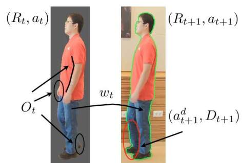
where $O_{t}$ denotes the subset of $R_{t}$ that is occluded from view in frame $t+1$, $D_{t+1}$ denotes the subset of the projected object that is disoccluded (comes into view) at frame $t+1$, $a^{d}_{t+1}:D_{t+1}\to\mathbb{R}^{k}$ is the radiance of the disoccluded region, and $w_{t}$ maps points that are not occluded in $R_{t}$ to $R_{t+1}$ in the next frame. The warp $w_{t}$ is a diffeomorphism on the un-occluded region $R_{t}\backslash O_{t}$ (it will be extended to all of $R_{t}$: see Section III-A for details), which is a transformation arising from viewpoint change and 3D deformation.

The region $R_{t}\backslash O_{t}$, is warped by $w_{t}$ and the dis-occlusion of the projected object, $D_{t+1}$, is appended to the warped region to form $R_{t+1}$. The relevant portion of the radiance, $a_{t}|(R_{t}\backslash O_{t})$ is transfered via the warp $w_{t}$ to $R_{t+1}$ (as usual brightness constancy), noise added, and then a newly visible radiance is obtained in $D_{t+1}$. The noise models deviation from brightness constancy (e.g., non-Lambertian reflectance, small illumination change, noise, etc…).

Organization of the rest of the paper: A template ($a_{0},R_{0}$) of the object is given. Our goal is, given an estimate of $R_{t}$, $a_{t}$, and $I_{t+1}$ to estimate $R_{t+1}$ in $I_{t+1}$. In Section III-A, we formulate an optimization problem to determine $w_{t}$ and the occlusion $O_{t}$ given $a_{t},R_{t}$, and $I_{t+1}$. In Section III-B, we formulate an optimization problem to determine the dis-occlusion $D_{t+1}$ given $w_{t}(R_{t}\backslash O_{t})$ and $I_{t+1}$. The joint energy for $w_{t}$ and $O_{t}$ presented in Section III-A involves an alternating optimization. In Section IV, we present a new general optimization scheme for energies defined on warps, which requires introducing a new Riemannian manifold and a novel Riemannian metric, a Sobolev-type region based metric, whose corresponding gradient descent we show has a coarse-to-fine property. This optimization scheme is a relevant sub-problem for the energy of interest in Section III-A, and the full optimization scheme for the joint energy in the warp and occlusion is presented in Section V-A. The optimization for the dis-occlusion energy is presented in Section V-B. Finally, in Section VI, we derive a recursive estimation procedure and integrate all steps. See Fig. 2 for a system overview.

template	target	warped template	occlusion map	occlusion removed
$(a_{t},R_{t})$	$I_{t+1}$	$a_{t}\circ w_{t},\,w_{t}(R_{t})$	$w_{t}(O_{t})$	$w_{t}(R_{t}\backslash O_{t})$
(a) Input		(b)

dis-occlusion	dis-occlusion added
$D_{t+1}$	($a_{t+1},R_{t+1}$)
(c)	(d)

Figure 2: Illustration of frame processing in our algorithm. (a): Estimate at frame $t$ of the shape and radiance $(a_{t},R_{t})$, and the next image $I_{t+1}$. (b): Simultaneous non-rigid warping and occlusion estimation is performed (first image: warped template $a_{t}\circ w_{t}$, second: boundary of warped template in $I_{t+1}$, third: warped occlusion $w_{t}(O_{t})$ determined, fourth: warped template with warped occlusion removed $w_{t}(R_{t}\backslash O_{t})$, fifth: boundary of $w_{t}(R_{t}\backslash O_{t})$). (c): Dis-Occlusion $D_{t+1}$ in $I_{t+1}$ determined from input $w_{t}(R_{t}\backslash O_{t})$. (d): Final shape and radiance $(a_{t+1},R_{t+1})$ in frame $t+1$ (adding dis-occlusion $D_{t+1}$ to $w_{t}(R_{t}\backslash O_{t})$). Shaded gray regions indicates not defined.

III Energy Formulation

This section concerns formulation of a joint energy for the warp of a given template to a subset to be determined in an image and the occluded subset of the template in the first sub-section, and in the subsequent sub-section, a formulation of an energy for the dis-occlusion.

III-A Joint Energy for the Warp and Occlusion

We model the warp $w_{t}$ as a diffeomorphism (smooth invertible non-rigid transformation) from $R_{t}\backslash O_{t}$ (the co-visible region) to an unknown target set (that must be determined) in the domain of $I_{t+1}$. An occlusion of region $R_{t}$ is the subset of $R_{t}$ that goes out of view in frame $t+1$. We compute occlusions as the subset of $R_{t}$ that does not register to $I_{t+1}$ under a viable warp. Thus, the occlusion depends on the warp, but to determine an accurate warp, data from the occluded region must be excluded, hence a circular problem. Therefore, occlusion detection and registration should be computed jointly.

We avoid subscripts $t$ for ease of notation in the rest of this section, and all sections until Section VI. We formulate the problem of given a region $R\subset\Omega$, the radiance $a:R\to\mathbb{R}^{k}$, and $I:\Omega\to\mathbb{R}^{k}$ to compute the occluded part $O$ of $R$, the warp $w$ defined on $R\backslash O$, and $w(R\backslash O)$ such that $I(x)=a(w^{-1}(x))+\eta(x)$ for $x\in w(R\backslash O)$ (where $\eta$ is noise modeled in (2)).

The warp $w$ is a diffeomorphism in the un-occluded region $R\backslash O$. For ease in the optimization, we consider $w$ to be extended to a diffeomorphism on all of $R$; the warp of interest will be the restriction to $R\backslash O$. We setup an optimization problem to determine $w$ so that $w(R\backslash O)$ is the object region in $I$, i.e., $a|R\backslash O$ should correspond to $I|w(R\backslash O)$ via the warp $w$. We thus formulate the energy (to be minimized in $O,w$) as

$$E_{o}(O,w;I,a,R) =\int_{R}f(w(x),x)\,\mathrm{d}x+\beta_{o}\mbox{Area}(O)$$ (3)

$$f(y,z) =\rho((I(y)-a(z))^{2})\bar{\chi}_{O}(y)$$ (4)

where $\beta_{o}>0$ is a weight, $\bar{\chi}_{O}(x)=1-\chi_{O}(x)$, $\chi_{O}$ is the characteristic function of $O$, and $\rho:\mathbb{R}\to\mathbb{R}$ is some monotonic function (e.g., $\rho(x)=x$ for a quadratic penalty or $\rho(x)=\sqrt{x+\varepsilon}$ where $\varepsilon>0$ for a robust penalty [41]; the choice of $\rho$ will depend on the actual noise model $\eta$ chosen in (2)). The first term penalizes deviation of the object radiance, $a$, to the pull-back of the image intensity $I|w(R)$ under $w$ onto the region $R$. The term $\bar{\chi}_{O}(x)$ implies that $w$ is only required to warp the radiance to match the image intensity $I$ in the un-occluded region $R\backslash O$. The occlusion area penalty is needed to avoid the trivial solution $O=R$. Given a moderate frame rate of the camera, it is realistic to assume that the occlusion is small in area compared to the object.

Due to the aperture problem, multiple warps $w$ can optimize the energy $E_{o}$, and typically a regularization term is added directly into the energy (e.g., for small warps as in optical flow [42], or for large warps [37]), changing the energy. Rather than regularizing the energy, we regularize the flow optimizing $E_{o}$ in a way that optimizes $E_{o}$ without changing it, leading to a favorable solution; this is described in Section IV.

III-B Energy Formulation of Dis-Occlusion

We now describe the energy formulation of the dis-occlusion $D_{t+1}\subset\Omega$ of the object at frame $t+1$ given the warped un-occluded part of the region $w_{t}(R_{t}\backslash O_{t})$ determined from the optimization of the energy in the previous section, and the image $I_{t+1}$. To determine the disoccluded region of the object (the region of the projected object that comes into view in the next frame that is not seen in the current template), it is necessary to make a prior assumption on the 3D object.

A realistic assumption is self-similarity of the 3D object’s radiance (that is, the radiance of the 3D object in a patch is similar to other patches). To translate this prior into determining the dis-occlusion of the object $D_{t+1}$, we assume that the image in the disoccluded region of the object is similar to parts of the image $I_{t+1}$ in $w_{t}(R_{t}\backslash O_{t})$, and for computationally efficiency, we assume similarity to close-by parts of the template. This is true in many cases, and is effective as shown in the experiments.

Although dis-occlusions in image $I_{t+1}$ are parts of the image that do not correspond to $I_{t}$ (i.e., an occlusion backward in time), these parts may be a dis-occlusion of the object or the background. It is not possible to determine without additional priors which dis-occlusions are of the object of interest. Our method works directly from the prior without having to compute a backward warp.

We now setup an optimization problem for the dis-occlusion. To simplify notation, we avoid subscripts in $D_{t+1}$ and $I_{t+1}$, and denote $R^{\prime}=w_{t}(R_{t}\backslash O_{t})$. The energy is

$$E_{d}(D)=-\int_{D}p(x)\,\mathrm{d}x+\beta_{d}\mbox{Area}(D)$$ (5)

where $D\subset\Omega\backslash R^{\prime}$, $p(x)\geq 0$ denotes the likelihood that $x\in\Omega\backslash R^{\prime}$ belongs to the dis-occluded region, and $\beta_{d}>0$ is a weight. The dis-occluded region, assuming a moderate camera frame rate, is small in area compared to the projected object, hence the penalty on area.

Let $\text{cl}(x)$ denote the closest point of $R^{\prime}$ to $x$, and let $B_{r}(x)$ denote the ball of radius $r$ about the point $x$. We choose $p(x)$ to have two components (see diagram in Fig. 3.): one that measures the fit of $I(x)$ to the local distribution of $I$ within $B_{r}(\text{cl}(x))\cap R^{\prime}$ versus the background $B_{r}(\text{cl}(x))\cap\{d_{R^{\prime}}>\varepsilon\}$ in $I$, and the second that measures nearness of $x$ to $R^{\prime}$. One choice of $p$ is

$$p(x)\propto\exp{\left[-\frac{d_{R^{\prime}}(x)^{2}}{2\sigma_{d}^{2}}+p_{\text{cl}(x),f}(I(x))-p_{\text{cl}(x),b}(I(x))\right]}$$ (6)

where $d_{R^{\prime}}(x)$ indicates the Euclidean distance from $x$ to $R^{\prime}$, $\sigma_{d}>0$ is a weighting factor, $p_{\text{cl}(x),f},\,p_{\text{cl}(x),b}$ are Parzen estimates of the intensity distribution of $I$ in $B_{r}(\text{cl}(x))\cap R^{\prime}$ (resp. $B_{r}(\text{cl}(x))\cap\{d_{R^{\prime}}>\varepsilon\}$) where $\varepsilon$ is chosen large enough so that the region includes some background beyond the dis-occlusion.

Figure 3: Diagram of quantities used in the likelihood $p(x)$ of a disoccluded pixel. The dark gray region is the dis-occlusion to be determined. Light gray region is $R^{\prime}$, region before the dis-occlusion is determined. A pixel $x$ within the band $\{0<d_{R^{\prime}}\leq\varepsilon\}$ is depicted, and its closest pixel to $R^{\prime}$, $\mbox{cl}(x)$. The green (blue) region is where the foreground (background) distribution $p_{\text{cl},f}(x)$ ($p_{\text{cl},b}(x)$) is determined.

IV Coarse-To-Fine Optimization of Energies Defined on Warps

In order to optimize $E_{o}$, we will apply an alternating scheme, alternating between optimization of $O$ and $w$, which will be presented in Section V. This section will focus on the general problem of optimizing an energy defined on warps of the form

$$E(w)=\int_{R}f(w(x),x)\,\mathrm{d}x$$ (7)

where $f:\Omega\times\Omega\to\mathbb{R}$. Note that this sub-problem is relevant in optimizing $E_{o}$. The optimization with respect to $w$ is done using a steepest descent scheme. Steepest descent depends on a Riemannian metric on the space of warps, $w$. The Riemannian metric is defined on infinitesimal perturbations of the warp $w$, and the metric controls the type of motions/deformations that are favored in optimizing the energy. We will design a novel Sobolev-type metric, and use it in the steepest descent of $E$.

The motivation for the design of this metric comes from the active contours literature [29, 31], where it was shown that Sobolev-type metrics defined on curves (boundaries of regions) result in flows that optimize the energy in a coarse-to-fine manner, initially optimizing the energy with respect to coarse perturbations, and then moving on to finer perturbations when coarse deformations no-longer optimize the energy. This coarse-to-fine behavior is done in an automatic fashion simply by using the Sobolev metric to compute the gradient of the energy. Motivated by this coarse-to-fine property, we design a new-Sobolev metric that is suited for energies defined on warps (rather than on curves in the active contour literature), that is, a region-based metric. The metric used in [29, 31] does not apply to the energy of interest in this paper as $E$ is defined on the space of warps (the point-wise correspondence of the interior is essential) rather than on boundaries of closed curves as the energies considered in [29, 31].

IV-A Sobolev Region-Based Metric and Gradient

We start by presenting some theoretical background so that the metric can be defined and the computation of the gradient of the energy with respect to the metric can be done. The space where our energy is defined is

$$M=\{w:R\to\Omega\subset\mathbb{R}^{2}\,:\,w:R\to w(R)\mbox{ is a diffeomorphism}\},$$ (8)

where $R\subset\Omega\subset\mathbb{R}^{2}$ is a compact set with smooth boundary (and thus also the range of $w$’s are compact and have smooth boundary). A diffeomorphism is a smooth invertible map whose inverse is also smooth. The range of $w\in M$ need not be all of $\Omega$, but rather an arbitrary subset of $\Omega$. We refer to $M$ as the space of parameterized regions since elements $w\in M$ parameterize regions $w(R)$ via the fixed region $R$. Note that the actual parameterization of a region is important as the energy of interest $E$ depends on the parameterization.

Infinitesimal perturbations of $w$ are given by smooth vector fields $h:R\to\mathbb{R}^{2}$, which form the tangent space to $w$ and is denoted $T_{w}M$. An infinitesimal perturbation of $w$ is $w_{\varepsilon}$, given by

$$w_{\varepsilon}(x)=w(x)+\varepsilon h(x).$$ (9)

Note that if $\varepsilon>0$ is small enough, then $w_{\varepsilon}\in M$, i.e., $w_{\varepsilon}$ is a diffeomorphism, which implies that $M$ is a manifold and thus, we may define a Riemannian metric on $T_{w}M$, which in turn allows us to define gradients of the energy. Perturbations $h$ are defined on $R$, and by right translation, i.e., $h\circ w^{-1}:w(R)\to\mathbb{R}^{2}$, they are also defined on $w(R)$. We now specify an inner product on $T_{w}M$, which makes $M$ a Riemannian manifold:

Definition 1 (Sobolev-type Inner Product on $M$).

The inner product on the set of perturbations of $w$ (i.e., the metric) that we consider is defined as follows:

$$\left<{h_{1}},{h_{2}}\right>_{w}=\mbox{avg}({\hat{h}_{1}})\cdot\mbox{avg}({\hat{h}_{2}})+\alpha\int_{w(R)}\mbox{tr}\left\{\nabla\hat{h}_{1}(x)^{T}\nabla\hat{h}_{2}(x)\right\}\,\mathrm{d}x$$ (10)

where $\alpha>0$, $\hat{h}:=h\circ w^{-1}$ when $h:R\to\mathbb{R}^{2}$, $\nabla\hat{h}_{1}(x)$ denotes the spatial Jacobian of $\hat{h}_{1}(x)$, tr denotes the trace of a matrix, $\,\mathrm{d}x$ is the area measure on $w(R)$, and

$$\mbox{avg}({\hat{h}})=\frac{1}{|w(R)|}\int_{w(R)}\hat{h}(x)\,\mathrm{d}x.$$ (11)

The first term in (10) uses the mean value of the perturbations rather than the $\mathbb{L}^{2}$ inner product of the perturbations as in standard Sobolev inner products [43]. This change is for convenience in the algorithm that we present to optimize $E$, and an easy decomposition of the gradient into orthogonal components as we shall see. The second term of (10) is the $\mathbb{L}^{2}$ inner product of the Jacobian of the perturbations.

The goal now is to define a gradient (or steepest) descent approach to minimize $E$. It should be noted that the gradient of an energy depends on the choice of inner product on the space of perturbations of the warp. The typical choice (either implicitly or explicitly) is the $\mathbb{L}^{2}$ inner product, but this does not have desirable properties for tracking applications. We therefore, compute the gradient with respect to the Sobolev inner product defined above (10). First, we state the definition of the gradient, which shows the dependence on the inner product:

Definition 2 (Gradient of Energy).

Let $E:M\to\mathbb{R}$, $w\in M$, $h\in T_{w}M$, and $\left<{},{}\right>_{w}$ denote the inner product on $T_{w}M$. The directional derivative of $E$ at $w$ in the direction $h$ denoted, $\,\mathrm{d}E(w)\cdot h$, is

$$\,\mathrm{d}E(w)\cdot h=\frac{\,\mathrm{d}{}}{\,\mathrm{d}{\varepsilon}}E(w+\varepsilon h)|_{\varepsilon=0}.$$ (12)

The gradient of $E$, denoted $\nabla_{w}E\in T_{w}M$, is the perturbation that satisfies the relation

$$\,\mathrm{d}E(w)\cdot h=\left<{\nabla_{w}E},{h}\right>_{w}$$ (13)

for all $h\in T_{w}M$.

In order to see intuitively how the choice of inner product affects the gradient, we give another interpretation of the gradient, i.e., it is a perturbation that maximizes the following ratio:

$$\frac{\,\mathrm{d}E(w)\cdot h}{\|h\|_{w}}$$ (14)

where $\|h\|_{w}=\sqrt{\left<{h},{h}\right>_{w}}$ is the norm induced by the inner product. That is, the gradient is a perturbation $h$ that maximizes the change in energy by perturbing in direction $h$ divided by the norm of the perturbation. Therefore, while it is often stated that the gradient is the direction that maximizes the energy the fastest, it is actually the direction that maximizes energy while minimizing its cost (measured by the norm). Since non-smooth perturbations cost a lot according to the Sobolev norm, they are not typically Sobolev gradients. Coarse perturbations are favored for Sobolev gradients when they can increase the energy. Note that moving in the negative gradient direction, $h=-\nabla_{w}E$, reduces the energy for any choice of $\alpha$.

The Sobolev gradient of $E$, $G=\nabla_{w}E$ is a linear combination of two (orthogonal) components, the translation and the deformation:

$$G(x)=\mbox{avg}({G})+\frac{1}{\alpha}\tilde{G}(x),\,x\in w(R)$$ (15)

where $\tilde{G}$ (which is independent of $\alpha$) satisfies the following Poisson PDE:

$$\begin{cases}-\Delta\tilde{G}(x)=f_{1}(x,w^{-1}(x))\det{(\nabla w^{-1}(x))}^{-1}-\mbox{avg}({f_{1}(\cdot,w^{-1}(\cdot)\det{(\nabla w^{-1}(\cdot))})^{-1}})&x\in w(R)\\ \nabla\tilde{G}(x)\cdot N=0&x\in\partial w(R)\\ \mbox{avg}({\tilde{G}})=0&\end{cases},$$ (16)

where $\Delta$ denotes the Laplacian, $N$ is the outward unit normal to $\partial w(R)$,

$$\mbox{avg}({G})=\int_{R}f_{1}(x,w^{-1}(x))\det{(\nabla w^{-1}(x))}^{-1}\,\mathrm{d}x,$$ (17)

and $f_{1}$ denotes the partial derivative of $f$ with respect to the first argument of $f$. Details of the derivations for these expressions can be found in Appendix A. The numerical scheme to solve (16) is given in Appendix B-A. Note that larger $\alpha$ (implying more spatial regularity) implies the gradient approaches a translation (the smoothest transformation), and smaller $\alpha$ implies a non-rigid deformation, which is spatially smooth and the amount of smoothness depends on the data.

IV-B Optimizing the Energy via Gradient Descent

The gradient flow to optimize $E_{o}$ is then given by the following partial differential equation

$$\begin{cases}\partial_{\tau}\phi_{\tau}(x)=-\nabla_{w}E(\phi_{\tau}(x))&x\in R\\ \phi_{0}(x)=x&x\in R\end{cases}$$ (18)

where $\tau$ indicates an artificial time parameter parameterizing the evolution of the warp $\phi_{\tau}:R\to\Omega$ at a given frame in the image sequence (not to be confused with the frame number $t$). The final converged $\phi_{\tau}$ is a local optimizer of the energy $E$. It should be noted that the above equation maintains that $\phi_{\tau}\in M$, i.e., that the final converged result is a diffeomorphism. This can be seen since $\nabla_{w}E$ is smooth (it is the solution of a Poisson equation and thus, $H^{2}$ [43]), and integrating a smooth vector field results in diffeomorphism using classical results [44] (and in particular [45] for first order Sobolev regularity), precise details for this fact are out of the scope of this paper.

In implementing the gradient flow (18), we are interested in the final converged region, and thus we keep track of $R_{\tau}=\phi_{\tau}(R)$. For numerical ease and accuracy, we keep track of $R_{\tau}$ using a level set method [46], although it is not required. We also keep track of the backward map $\phi_{\tau}^{-1}$, which is needed to evaluate the gradient $\nabla_{w}E(\phi_{\tau}(x))$.

The level set function will be denoted $\Psi_{\tau}:\Omega\to\mathbb{R}$. Its evolution is described by a transport PDE. The backward map $\phi_{\tau}^{-1}$ also satisfies a transport equation. Therefore, the optimization of $E$ is given by the coupled PDE:

$$\Psi_{0}(x) =d_{R}(x),\,x\in B_{2}(R)$$ (19)

$$\phi_{0}^{-1}(x) =x,\,x\in R$$ (20)

$$R_{0} =R$$ (21)

$$G_{\tau} =\nabla_{w}E(\phi_{\tau})$$ (22)

$$\partial_{\tau}\phi_{\tau}^{-1} =\nabla\phi_{\tau}^{-1}(x)\cdot G_{\tau}(x),x\in R_{\tau}$$ (23)

$$\partial_{\tau}\Psi_{\tau} =\nabla\Psi_{\tau}(x)\cdot G_{\tau}(x),x\in B_{2}(R_{\tau})$$ (24)

$$R_{\tau} =\{\Psi_{\tau}<0\}$$ (25)

where $\partial_{\tau}$ denotes partial with respect to $\tau$, and $B_{2}(R_{\tau})=\{x\in\Omega:|d_{R_{\tau}}(x)|\leq 2\}$ where $d_{R_{\tau}}$ is the signed distance function of $R_{\tau}$. The region $R_{\tau}$ is updated in direction of minus the gradient of $E$, $-G_{\tau}:R_{\tau}\to\mathbb{R}^{2}$ via the level set evolution. Note $G_{\tau}$ is extended to $B_{2}(R_{\tau})$ as in narrowband level set methods. The backward warp $\phi_{\tau}^{-1}:R_{\tau}\to R$ is computed by flowing the identity map along the velocity field $-G_{\tau}$ up to time $\tau$, and this is accomplished by the transport equation (23). At convergence (when $E$ does not decrease), we denote this time $\tau_{\infty}$, $w=(\phi^{-1}_{\tau_{\infty}})^{-1}:R\to R_{\tau_{\infty}}$ is a local optima of $E$, and $R_{\tau_{\infty}}=w(R)$ is the region matched in the image $I$.

The evolution above is automatically coarse-to-fine for any choice of $\alpha$, that is, the gradient descent favors coarse motions/deformations initially before transitioning to more finer scale deformations. See Figure 5 in Sub-Section IV-D for an experimental verification of this property.

IV-C Parameter Independent Optimization

One of the advantages of the particular form of the Sobolev-type metric chosen in (10) besides the coarse-to-fine property is that one can eliminate the need for choosing the parameter $\alpha$, while optimizing $E$. One can take $\alpha\to\infty$, in which case $G\to\mbox{avg}({G})$, a translation motion. One can optimize by translating in the direction $-G=-\mbox{avg}({G})$ when $\alpha\to\infty$, until convergence. At convergence, $\mbox{avg}({G})=0$, then one can evolve the warp infinitesimally in the negative gradient $-G=-\tilde{G}/\alpha$ direction for any finite $\alpha$. Since the gradient depends only on $\alpha$ by a scale factor, the choice of $\alpha$ is just a time re-parameterization of the evolution, not changing the geometry of the evolution, and does not impact the final converged warp nor the converged region. The algorithm to optimize $E$ that is not dependent on the choice of $\alpha$ is summarized in the following steps:

1. Perform the initializations (19)-(21).

2. Repeat the evolution (22)-(25) with $\alpha\to\infty$, in which case $G_{\tau}=\mbox{avg}({G_{\tau}})$, until convergence (when $\mbox{avg}({G_{\tau}})=0$).

3. Perform one time step (22)-(25) with the deformation of $G_{\tau}\propto\tilde{G}_{\tau}$ (one may choose $\alpha=1$, but any choice would give the same result).

4. Repeat Steps 2-3 until convergence (when $E$ does not decrease).

The procedure above optimizes with respect to translations first until convergence, then optimizes with respect to deformations that are not translations (favoring coarse motions/deformations if they optimize the energy), and the process is iterated. This results in a scheme that is independent of a regularity parameter $\alpha$, and that favors a coarse-to-fine evolution (like the gradient descent with any fixed $\alpha$) of the region $R_{\tau}$ and coarse-to-fine motion/deformation estimation.

IV-D Discussion

We now discuss the relation of our approach to classical optical flow and tracking approaches, namely the approach by Lucas and Kanade [47] and Horn and Schunck [42].

Since there are multiple possible solutions optimizing $E$ (that contains just data fidelity), regularization must be used to determine a viable solution. The approach in [47] is to restrict the possible warps to a smaller set rather than the space of diffeomorphisms, i.e., translations, affine motions, or other parametric groups. While providing less ambiguity in determining a unique optimizer of $E$, this restricts the possible warps $w$ and thus also the shape of the region. One may consider optimizing $E$ with respect to translations first, thus getting a coarse estimate of the desired region in image $I$, then resort to optimizing in more fine transformations, e.g., Euclidean transformations (i.e., translations and rotations), then affine transformations. However, one may go up to the projective group, and then it becomes unclear what group to choose to optimize further. The algorithm that we have presented to optimize $E$ optimizes the energy by using coarse perturbations initially, it then transitions continuously and automatically to more finer-scale perturbations, in fact, it transitions through all possible scales of motions/deformations, eliminating the need to choose groups of motions to optimize. This property of Sobolev-type metrics for contours was shown analytically in particular cases using a Fourier analysis in [31]. In this work, since we work with regions, the property is harder to show analytically since the Fourier basis would need to be derived using the eigenfunctions of the Laplacian defined on a region, difficult to perform analysis analytically. We therefore demonstrate the property in an experiment.

The method of optical flow computation in [42] deals with multiple possible optimizers of $E$ by changing the original energy by adding regularization of the warp directly into the energy; indeed the energy for infinitesimal warps is

$$E_{HS}(v;a,I,R)=\int_{R}|I(x)-a(x)+\nabla a(x)\cdot v(x)|^{2}\,\mathrm{d}x+\gamma\int_{R}|\nabla v(x)|^{2}\,\mathrm{d}x.$$ (26)

An advantage of this approach over [47] is that, the motions/deformations are not restricted to finitely parameterized motions. The parameter $\gamma$ controls the scale of the estimated motion (large $\gamma$ implying coarse motion, and small $\gamma$ implying finer motion). One can deform the region $R$ by $v$ infinitesimally to obtain $R_{\tau}$, then recalculate $v$ based on the warped appearance $a\circ\phi_{\tau}^{-1}$, and iterate the process to determine the region of the object in the next frame. While the procedure allows the cumulative warp $w$ to be an arbitrary diffeomorphism and therefore obtain arbitrarily shaped regions, the technique relies on the choice of the parameter $\gamma$: large $\gamma$ yields only coarse approximations of the region shape, and small $\gamma$ yields finer details of shape, but is likely to be trapped in fine details of the image before reaching the desired region of interest. There is no principled way to choose $\gamma$, and no one scale of motions/deformations, that is no one $\gamma$, is sufficient. Further, the iterative procedure described does not optimize an energy for the warp $w$ (although each iteration minimizes an $E_{HS}$ for an infinitesimal warp).

One ad-hoc solution to the dilemma of choosing $\gamma$ is to attempt a coarse-to-fine scheme by starting with $\gamma$ large until the region in the procedure discussed converges, reduce $\gamma$ and then deform the region until convergence, reduce $\gamma$, etc., (which is the scheme considered in our preliminary conference paper [40]). While the procedure solves issue of the choice of $\gamma$ and is coarse-to-fine, our proposed algorithm has three advantages. First, our scheme does not rely on an ad-hoc scheme to reduce the parameter $\gamma$. Second, our scheme automatically and continuously traverses through all possible scales of motions/deformations favoring roughly coarse-to-fine transition, whereas the ad-hoc scheme only traverses through a discrete number of scales (chosen by the scheme to reduce $\gamma$) and the transition is not automatic. Reducing $\gamma$ monotonically in the ad-hoc scheme may not always be beneficial (e.g., when new coarse structure is “discovered” from the data during evolution and larger $\gamma$ is then needed), our new scheme chooses the appropriate scale of deformation automatically from computation of the gradient, generally favoring coarse-to-fine. There is no added complication in our new Sobolev descent: the gradient has similar structure as the velocity in Horn & Schunck, both have similar numerical implementation, and same efficiency. Our scheme is thus much more convenient for practical applications. Lastly, our scheme is minimizing the objective energy $E$, while the ad-hoc scheme does not necessarily minimize an energy.

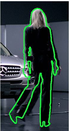
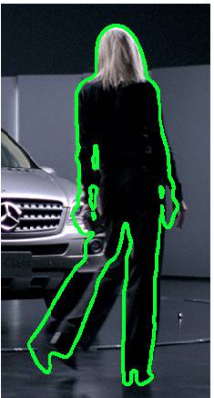
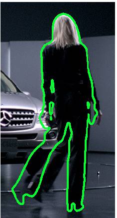
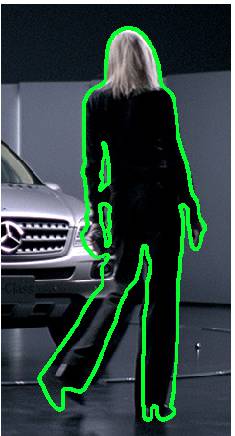
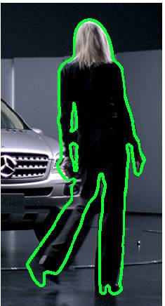
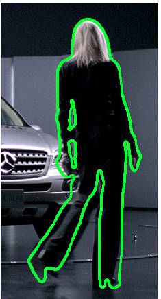
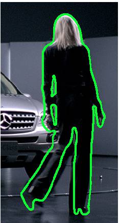
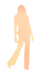
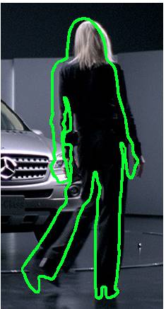
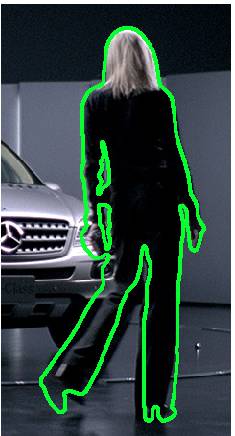
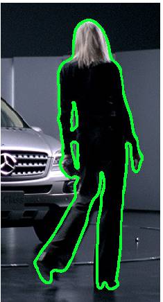
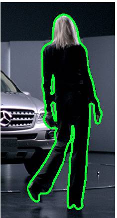
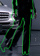
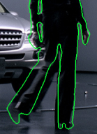
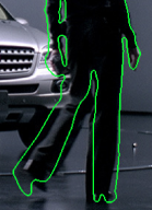
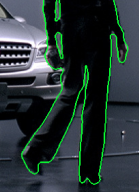
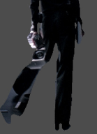
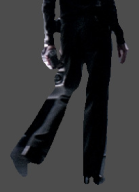
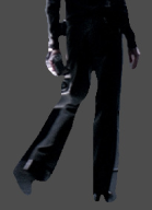
We illustrate the coarse-to-fine behavior of the region-based Sobolev gradient descent by matching a template of the object (woman) obtained from image 1 to image 2 shown in Fig. 4, where there are both coarse-scale and fine-scale deformations. The evolution (at various snapshots and ran until convergence) of region-based Sobolev and a Horn and Schunck approach described above with varying $\gamma$ is shown in Fig. 5. Final objects detected with these schemes in a zoomed region of interest is shown in Fig. 6. The displacement between two time instances $\tau_{i}$ and $\tau_{i+1}$, that is, $d_{\tau_{i},\tau_{i+1}}(x)=\phi_{\tau_{i}}\circ\phi_{\tau_{i+1}}^{-1}(x)-x$, is is shown in optical flow code [48] (the color indicates direction and darkness indicates magnitude; magnitude should not be compared across images as they are re-scaled in each image) in Fig. 5. Notice that the region-based Sobolev moves according to coarse motions (nearly constant color in the visualization) before gradually resorting to finer-scale deformations whereas the Horn & Schunck approach has roughly the same scale of motions/deformation at all stages of the evolution for each $\gamma$. Small $\gamma$ does not capture regions of coarse deformation and gets stuck in intermediate structures. Larger $\gamma$ captures regions of coarse deformation, but regions of finer scale motion (e.g., the legs) are not captured. The Sobolev descent moves from coarse-to-fine deformations, and thus captures both regions of coarse and fine deformation.

Figure 4: Images $I_{1}$ (left) and $I_{2}$ (middle) used in the experiment in Figure 5, and an overlay of $I_{1}$ on $I_{2}$ to show the motion/deformation between frames, which is non-rigid and contains both coarse and fine motion/deformations.

Energy regularization, $\gamma=10$
Energy regularization, $\gamma=100$
Energy regularization, $\gamma=500$
Coarse-to-Fine Region-Based Sobolev Descent (Parameter-free)

Figure 5: Coarse-to-Fine Behavior of Region-Based Sobolev Descent. Matching a template (obtained from $I_{1}$) to $I_{2}$ from Figure 4 using regularization of the velocity field in the energy, and Sobolev descent. In each row, the evolution (until convergence) is shown. [First four images]: $\partial R_{\tau}$ on $I_{2}$ for various snapshots $\tau$. [Last three images]: displacement of object between adjacent snapshots (in optical flow color code). Small $\gamma$ favors fine deformations and is sensitive to intermediate structures, whereas large $\gamma$ favors only coarse deformations and cannot capture regions with fine-scale deformations, e.g., legs. Sobolev descent captures all scales of deformation without being sensitive to intermediate structures.

Figure 6: Zoom of final converged results of experiment of Figure 5. [Top row]: boundary of converged region on $I_{2}$, [Bottom row]: cutout of object in $I_{2}$. [Left]: energy regularization $\gamma=10$, [Middle-left]: energy regularization $\gamma=100$, [Middle-right]: energy regularization $\gamma=500$, [Right]: region-based Sobolev. Notice that small $\gamma$ misses regions of coarse motion, larger $\gamma$ obtains regions of coarse motion, but misses regions where finer deformation occurs. Sobolev obtains both coarse and fine deformations.

V Occlusion/Dis-occlusion Computation and Alternating Optimization

We now describe the alternating optimization scheme to optimize $E_{o}$, combining the coarse-to-fine optimization scheme described in the previous section, and optimization in the occlusion, which we describe next. We then present the optimization scheme to determine the dis-occlusion.

V-A Joint Occlusion and Warp Optimization

Note that given an estimate $w$, one can solve for a global optimizer of the energy $E_{o}$. Indeed, the energy can be written as

$$E_{o}(O|w;I,a,R)=\int_{R\backslash O}\rho((I(w(x))-a(x))^{2})\,\mathrm{d}x+\int_{O}\beta_{o}\,\mathrm{d}x,\,O\subset R.$$ (27)

The optimization problem can be thought of as an assigment problem where points $x\in R$ are assigned to the occlusion $O$ or the co-visible region $R\backslash O$. If $x$ is assigned to $O$, then it adds to the energy an amount $\beta_{o}$, whereas, if it is assigned to $R\backslash O$, it adds to the energy an amount $\rho((I(w(x))-a(x))^{2})$. Therefore to minimize the energy, we assign pixels to the occlusion based on

$$O =\{x\in R\,:\,\rho((I(w(x))-a(x))^{2})>\beta_{o}\}$$ (28)

$$=w^{-1}\{x\in w(R)\,:\,\rho((I(x)-a(w^{-1}(x))^{2}))>\beta_{o}\},$$ (29)

which is a global optimizer of $E_{o}$ conditioned on $w$.

The alternating scheme to optimize $E_{o}$ in both $O$ and $w$ is then a modification of the scheme presented in Sub-Section IV-B to update the occlusion during the evolution. The scheme is as follows:

$$\Psi_{0}(x) =d_{R}(x),\,x\in B_{2}(R)$$ (30)

$$\phi_{0}^{-1}(x) =x,\,x\in R$$ (31)

$$R_{0} =R$$ (32)

$$\tilde{O}_{0} =\emptyset$$ (33)

$$G_{\tau} =\nabla_{w}E(\phi_{\tau}|O_{\tau},R_{\tau},I)$$ (34)

$$\partial_{\tau}\phi_{\tau}^{-1} =\nabla\phi_{\tau}^{-1}(x)\cdot G_{\tau}(x),x\in R_{\tau}$$ (35)

$$\partial_{\tau}\Psi_{\tau} =\nabla\Psi_{\tau}(x)\cdot G_{\tau}(x),x\in B_{2}(R_{\tau})$$ (36)

$$R_{\tau} =\{\Psi_{\tau}<0\}$$ (37)

$$\tilde{O}_{\tau} =\{x\in R_{\tau}\,:\,\rho((I(x)-a(\phi_{\tau}^{-1}(x))^{2}))>\beta_{o}\},$$ (38)

where $\tilde{O}_{\tau}$ indicates the current estimate of the warped occlusion $O_{\tau}$, i.e., $\tilde{O}_{\tau}=\phi_{\tau}(O_{\tau})$. Note that only $\tilde{O}_{\tau}$ is needed to compute the gradient $G_{\tau}$, and thus we do not explicitly compute $O_{\tau}$. Note that $G_{\tau}$ is specified by $\mbox{avg}({G_{\tau}})$ and $\tilde{G}_{\tau}$, where $\tilde{G}_{\tau}$ satisfies

$$\begin{cases}-\Delta\tilde{G}_{\tau}(x)=f_{1}(x,\phi_{\tau}^{-1}(x))\det{(\nabla\phi_{\tau}^{-1}(x))}^{-1}-\mbox{avg}({f_{1}(\cdot,\phi_{\tau}^{-1}(\cdot))\det{(\nabla\phi_{\tau}^{-1}(\cdot))}^{-1}})&x\in R_{\tau}\\ \nabla\tilde{G}_{\tau}(x)\cdot N=0&x\in\partial R_{\tau}\\ \mbox{avg}({\tilde{G}_{\tau}})=0&\end{cases}.$$ (39)

where

$$\mbox{avg}({G_{\tau}})=\int_{R}f_{1}(x,\phi_{\tau}^{-1}(x))\det{(\nabla\phi_{\tau}^{-1}(x))}^{-1}\,\mathrm{d}x,$$ (40)

and

$$f_{1}(x,\phi_{\tau}^{-1}(x)) =\rho^{\prime}(|I(x)-a_{\tau}(x))|^{2})(I(x)-a_{\tau}(x))\nabla I(x)\chi_{\tilde{O}_{\tau}}(x),\quad x\in R_{\tau}$$ (41)

$$a_{\tau}(x) =a(\phi_{\tau}^{-1}(x)),\quad x\in R_{\tau}$$ (42)

Discretization of (30)-(38) and numerical implementation is given in Appendix B.

Let $\tau=\tau_{\infty}$ be the time of convergence, $R_{\tau_{\infty}}$ - a warping of $R$ includes a warping of the occluded region $O_{\tau_{\infty}}$, and thus the warping of the un-occluded region is $w(R\backslash O_{\tau_{\infty}})=R^{\prime}_{{}_{\tau_{\infty}}}=R_{{}_{\tau_{\infty}}}\backslash\tilde{O}_{{}_{\tau_{\infty}}}$, and does not include the disoccluded region, which is computed in the next section from $R^{\prime}_{{}_{\tau_{\infty}}}$. To ensure spatial regularity of $R^{\prime}_{{}_{\tau_{\infty}}}$, at convergence of (30)-(38), we induce spatial regularity into $O_{\tau_{\infty}}$ by using the estimate

$$\tilde{O}_{\tau_{\infty}} =\{x\in R_{\tau_{\infty}}\,:\,(G_{\sigma}\ast\mbox{Res})(x)>\beta_{o}\}$$ (43)

$$\mbox{Res}(x) =\rho((I(x)-a(\phi_{\tau_{\infty}}^{-1}(x)))^{2})$$ (44)

where $G_{\sigma}$ denotes an isotropic Gaussian kernel.

Fig. 7 shows the evolution (30)-(38) on an example, and the final co-visible region $R^{\prime}_{{}_{\tau_{\infty}}}$.

Figure 7: Occlusion estimation and warping. [Top to bottom]: Beginning ($\tau=0$), intermediate, and final stages of evolution. [$1^{\text{st}}$ column]: radiance $a_{\tau}$, [$2^{\text{nd}}$]: target image $I$ and boundary of $R_{\tau}$, [$3^{\text{rd}}$]: velocity $-G_{\tau}$, [$4^{\text{th}}$]: occlusion estimation Res at time $\tau$, [$5^{\text{th}}$]: optical flow color code. The final occluded region is shown in Fig. 2(b).

V-B Dis-Occlusion Optimization

We show how to optimize the dis-occlusion energy $E_{d}$ (5). The global minimum of $E_{d}$ is computed in a thresholding step from the likelihood $p$. Since $p$ decreases exponentially with distance to $R^{\prime}$, we assume that $D\subset\{0<d_{R^{\prime}}<\varepsilon\}$. The dis-occlusion is computed as

$$D=\{x\,:\,d_{R^{\prime}}(x)\in(0,\varepsilon],(G_{\sigma}\ast p)(x)>\beta_{d}\}$$ (45)

where $\sigma=0$ corresponds to the global optimum, but to ensure spatial regularity of $D$, we choose $\sigma>0$. The choice of $\beta_{d}$ is based on the frame-rate of the camera and the speed of the object (the more the speed and the less the frame-rate, the smaller $\beta_{d}$). Fig. 8 shows an example of $p$, the dis-occlusion detected, and the final estimate of the region.

Computation of $d_{R^{\prime}}$ in $\{0<d_{R^{\prime}}<\varepsilon\}$ is done efficiently with the Fast Marching Method [49], and $\mbox{cl}(x)$ at each point is simultaneously propagated as the front in the Fast Marching Method evolves. Then $p$ is readily computed.

Figure 8: Illustration of disocclusion detection. [$1^{\text{st}}$]: warped un-occluded radiance defined on $R^{\prime}$ (after occlusion and deformation computation), [$2^{\text{nd}}$]: target image $I$, [$3^{\text{rd}}$]: likelihood of dis-occlusion map $p$ (defined in $B_{R^{\prime}}(\varepsilon)$), [$4^{\text{th}}$]: computed dis-occlusion $D$ (white), and [$5^{\text{th}}$]: final radiance. Boundary of final region super-imposed on $I$ is in Fig. 2 (d).

VI Filtering Radiance Across Frames

We integrate the results of occlusion/deformation estimation and dis-occlusion estimation into a final estimate of the shape and radiance in each frame. To deal with modeling noise (specified in (2)), we filter the radiance in time.

Given the image sequence $I_{t},\,t=1\ldots,N$ and an initial template $R_{0}\subset\Omega,\,a_{0}:R_{0}\to\mathbb{R}^{k}$, the final algorithm is as follows. For $t=1,\ldots,N$, the following steps are repeated:

1. Compute the warping of $R_{t-1}$ and $O_{t-1}$: $w_{t-1}(R_{t-1})$ and $w_{t-1}(O_{t-1})$, resp., and $a_{t}^{\prime}=a_{t-1}\circ w_{t-1}^{-1}$ defined on $w_{t-1}(R_{t-1})$ using the optimization scheme described in Section V-A with input $R_{t-1},a_{t-1}$ and $I_{t}$.

2. Given $R^{\prime}_{t}=w_{t-1}(R_{t-1})\backslash w_{t-1}(O_{t-1})$, the warping of the un-occluded part of $R_{t-1}$, and the image $I_{t}$, compute the dis-occlusion $D_{t}$ using (45). The estimate of $R_{t}$ is then $R_{t}^{\prime}\cup D_{t}$.

3. The radiance is then updated as

   $$\!\!a_{t}(x)=\begin{cases}(1-K_{a})a_{t}^{\prime}(x)+K_{a}I_{t}(x)&x\in R_{t}^{\prime}\\ I_{t}(x)&x\in D_{t}\end{cases}$$ (46)

   where $K_{a}\in[0,1]$ is the gain.

The averaging of the warped radiance and the current image (46) combats modeling noise $\eta$ in (2). In practice, $K_{a}$ is chosen large if the image is reliable (e.g., no specularities, illumination change, noise, or any other deviations from brightness constancy), and small otherwise.

VII Experiments and Comparisons

We demonstrate our method on a variety of videos that contain self-occlusions/disocclusions. All examples shown have over 100 frames. To demonstrate that occlusion/dis-occlusion modeling aids joint shape/appearance tracking, we compare to Adobe After Effects CS6 2013 (AAE) (based on [14], but significantly extended over several years), which employs localized joint shape and appearance information without explicit occlusion modeling. Note that AAE has an interactive component to correct errors in the automated component; we compare to the automated component to show less interaction would be required with our approach. To show advantages over tracking using global statistics, we compare to Scribbles [4] (publicly available code), which is a state-of-the-art technique that employs global statistics in addition to other advanced techniques.

Parameters are chosen as: $\sigma=5$ in (45) and (43), $\sigma_{d}=100$ in the likelihood, $p$ in (6), the band thickness for the domain of $p$ is $\varepsilon=30$, and the radius of $B_{r}$ in $p_{f,x}$ and $p_{b,x}$ is $r=3\varepsilon$ (i.e., a $6\varepsilon\times 6\varepsilon$ window). The threshold for the occlusion stage is $\beta_{o}=\mbox{Res}_{min}+0.3\times(\mbox{Res}_{max}-\mbox{Res}_{min})$ where $\mbox{Res}_{max}$ ($\mbox{Res}_{min}$) denotes the maximum (minimum) value of smoothed residual. The threshold for the dis-occlusion stage is $\beta_{d}=0.5$ when $p$ is normalized to be a probability. The gain in the radiance update (46) is $K_{a}=0.8$. Most parameters can be fixed for the whole video, and work on a wide range. Most significant parameters are the $\beta$’s, and sensitivity analysis is shown later (near the end of the Section).

The first experiment (Fig. 9) shows that occlusion and dis-occlusion modeling is vital. As the man in the sequence walks forward, his legs, arms and back are self-occluded/disoccluded. Ignoring occlusions (setting $\tilde{O}_{\tau}=\emptyset$ in Section V-A) and dis-occlusion detection, the shape is inaccurate (first row). Using occlusion modeling but not dis-occlusions (second row), it is possible to discard the portion of the background between the legs, and the occluded right hand in the first frame is removed. Using the dis-occlusion modeling but not occlusions (third row), disoccluded parts of the body are detected. However, irrelevant regions of the background (that can be removed in the occlusion stage) are captured. Best results (last row) are achieved when both the occlusion and dis-occlusions are modeled. The fourth row shows the result of Scribbles, which has trouble discriminating between face and the background, which share similar radiance. The fifth row shows the result of Adobe After Effects 2013 (AAE), which captures irrelevant background.

Figure 9: Modeling Occlusions/Dis-Occlusions is Necessary. [$1^{\text{st}}$ row]: occlusion/dis-occlusion detection are turned off in our method. [$2^{\text{nd}}$]: occlusion modeling done, but not dis-occlusions in our method. [$3^{\text{rd}}$]: dis-occlusions detected but not occlusions. [$4^{\text{th}}$]: result of Scribbles. [$5^{\text{th}}$]: result of AAE. [$6^{\text{th}}$]: accurate tracking when both occlusion and dis-occlusion modeling is performed (our final result).

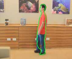
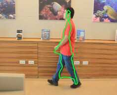
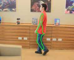
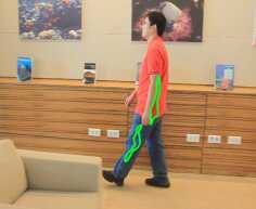
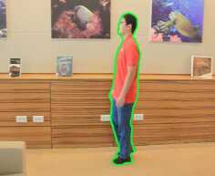
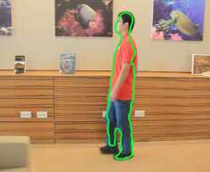
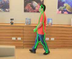
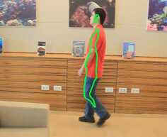
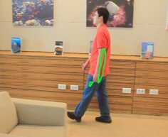
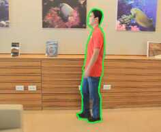
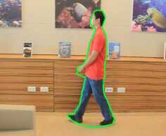
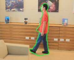
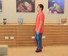
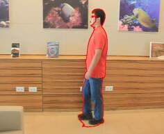
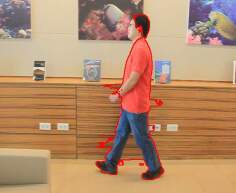
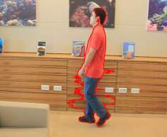
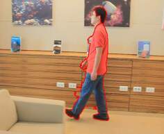
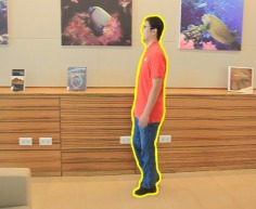
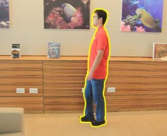
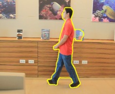
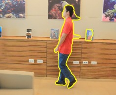
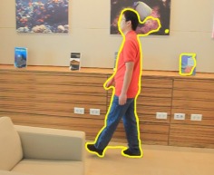
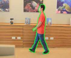
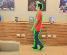
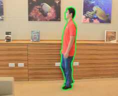
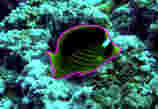
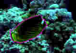
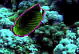
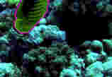
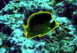
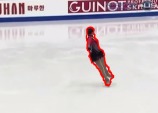
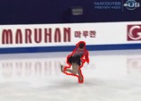
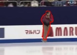
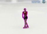
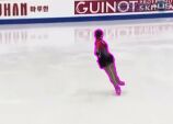
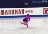
Fig. 10 shows tracking of a fish and a skater. When foreground/ background global histograms are easily separable, Scribbles performs well, and when occlusions are minor AAE, performs well as does the proposed method.

Figure 10: Distinctive foreground/background global statistics. [Top]: [4], [Middle]: AAE, [Bottom]: proposed method. When fore/background global statistics are separable, [4], and AAE, for minor occlusions, performs well.

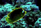
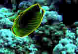
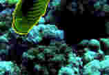
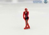
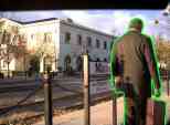
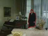
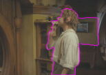
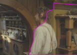
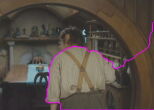
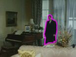
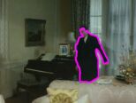
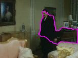
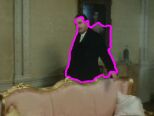
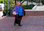
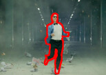
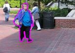
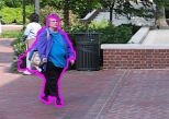
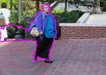
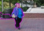
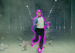
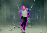
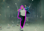
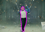
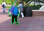
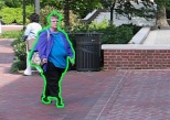
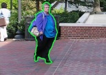
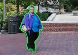
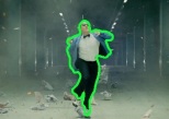
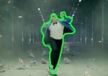
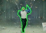
In Fig. 11, we have tested our algorithm on challenging video (more than 100 frames per sequence) exhibiting self-occlusions and dis-occlusion (crossing legs, viewpoint change, rotations in depth), complex object radiance and background in which it becomes difficult to discriminate between foreground and background global statistics (e.g., the woman’s pants have same radiance as car tires). Deviations from brightness constancy are clearly visible (small illumination change, specular reflections, and even shadows). The latter are handled with our dynamic radiance update. In these sequences, Scribbles and Adobe After Effects 2013 (AAE) have trouble discriminating between object and background which share portions of similar intensity, and occlusions (e.g., crossing of legs). In the “Lady Mercedes,” sequence (top left), after a few frames, Scribbles can only track the head of the lady. This is because the lady’s clothing shares similar intensity as the tires of the car and some of the background. Thus, the tracker confuses the clothing with the background and only tracks the head, which has different statistics from the rest of the images. Our method is able to capture the shape of the objects quite well (quantitative assessment is in Table I). The man at the station (top right group) at the fourth column shows a limitation of our dis-occlusion detection: dis-occluded parts of the object that do not share similar radiance as the current template (sole of shoe) are not detected. A variety of other videos are processed, and our method performs quite well.

Figure 11: Occlusions/dis-occlusions, violations of brightness constancy, and foreground/background not easily separable. [Top]: Scribbles, [Middle]: Adobe After Effects 2013, [Bottom]: proposed method. Methods based on foreground/background image statistic discrimination leak into the background. Note 4 (out of about 100-200) frames are selected for display in each sequence (see video on website).

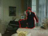
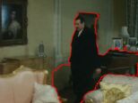
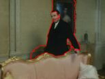
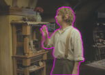
Sequence	Scribbles [4]	Adobe Effects 2013 [14]	Ours
Library	0.8926	0.9193	0.9654
Fish	0.9239	0.9513	0.9792
Skater	0.8884	0.6993	0.9086
Lady	0.2986	0.8243	0.9508
Station	0.5367	0.8258	0.9216
Hobbit	0.7312	0.5884	0.9335
Marple	0.6942	0.8013	0.9186
Lady 2	0.7457	0.7909	0.9584
Psy	0.6163	0.8845	0.9329

TABLE I: Quantitative performance analysis. Average F-measure (over all frames) computed from ground truth are shown. Larger F-measure means better performance.

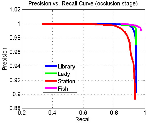
In Figure 12, we show a quantitative analysis of the sensitivity of the key parameters of the proposed method. We analyze the sensitivity of the thresholds $\beta_{o}$ and $\beta_{d}$ in the occlusion and disocclusion detection stages using an precision / recall (PR) curve. For four image sequences, we choose a pair of images so that significant occlusion and disocclusion are present between the frames, and significant deformation and motion is present. Typically, the pair is separated by 5 frames on these sequences that have a frame rate of 30 frames per second. Given a hand cutout in the first frame, we run our algorithm (both occlusion and disocclusion stages) to obtain the cutout in the next frame. The first image in Figure 12 shows the PR curve as the parameter $\beta_{o}$ is varied between its valid range (the minimum value of the residual, Res, and its maximum value), and the threshold of the disocclusion stage $\beta_{d}$ is kept fixed. The second image in Figure 12 shows the precision / recall curve as the parameter $\beta_{d}$ in the disocclusion stage is varied between its valid range (the minimum and maximum value of $p$), and the threshold in the occlusion stage $\beta_{o}$ is kept fixed. Note high precision and recall is maintained for a wide range of thresholds.

Figure 12: Sensitivity of Key Parameters. The figure shows a quantitative assessment of the sensitivity of the key parameters (i.e., thresholds), $\beta_{o}$ and $\beta_{d}$, of the proposed algorithm for the occlusion and disocclusion stages in the sequences above. The Precision/Recall curves indicate that the parameters are robust to a wide range of thresholds that result in high values of precision and recall.

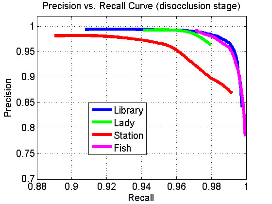
Lastly, we state the running time of our algorithm on a standard Intel 2.8GHz dual core processor. Note that the speed will depend on a variety of factors such as the size of the object and amount of deformation between frames. On HD 720 video, it is on average 8 seconds per frame for sequences in Fig. 11 (in C++), while AAE takes 1 second. Speed-ups are possible, e.g., the joint velocity and occlusion computation can be sped up using a multi-scale procedure.

VIII Conclusion

The proposed technique for shape tracking is based on jointly matching shape and complex radiance (defined as a function on the region) of the object across frames. Self-occlusions and dis-occlusions pose a challenge for joint shape/appearance tracking, which were modeled and computed in a principled framework in this work.

In order to compute self-occlusions and the warp of a template to the next frame, a joint energy was formulated, and a novel general optimization scheme was derived that has an automatic coarse-to-fine property, which is extremely useful in tracking. The method was based on constructing a novel infinite dimensional Riemannian manifold of parameterized regions and a novel Sobolev-type metric. The optimization scheme is a gradient descent with respect to the Sobolev-type metric, and empirical verification of the coarse-to-fine property was given.

Experiments demonstrated the criticality of modeling occlusions and dis-occlusions. Comparison to recent methods built on global image statistics foreground/background separation and joint shape/appearance modeling without occlusion modeling demonstrated the effectiveness of the proposed algorithm in situations of complex object/background radiance, and self-occlusions/dis-occlusions.

Future work includes full occlusions of the object by other objects, and improving dis-occlusion detection.

Appendix A Computing Region-Based Sobolev Gradients

We now show how to compute the gradient of an energy with respect to the Sobolev inner product defined in (10). For generality, we compute the gradient of

$$E(w)=\int_{R}f(w(x),x)\,\mathrm{d}x$$ (47)

where $f:\mathbb{R}^{2}\times\mathbb{R}^{2}\to\mathbb{R}$. The directional derivative in the direction $h:R\to\mathbb{R}^{2}$ is

$$\,\mathrm{d}E(w)\cdot h =\int_{R}f_{1}(w(x),x)\cdot h(x)\,\mathrm{d}x$$ (48)

$$=\int_{w(R)}f_{1}(x,w^{-1}(x))\cdot h\circ w^{-1}(x)\det{(\nabla w(x))}\,\mathrm{d}x$$ (49)

and since by definition $\,\mathrm{d}E(w)\cdot h=\left<{G},{h}\right>_{w}$ for all $h\in T_{w}M$, where $G=\nabla_{w}E$ is the gradient with respect to the Sobolev inner product, we have that

$$\int_{w(R)}f_{1}(x,w^{-1}(x))\cdot\hat{h}(x)\det{(\nabla w(x))}\,\mathrm{d}x=\mbox{avg}({G})\cdot\mbox{avg}({\hat{h}})+\alpha\int_{w(R)}\mbox{tr}\left\{\nabla G(x)^{T}\nabla\hat{h}(x)\right\}\,\mathrm{d}x$$ (50)

By integrating by parts, one finds that

$$\int_{w(R)}f_{1}(x,w^{-1}(x))\cdot\hat{h}(x)\det{(\nabla w(x))}\,\mathrm{d}x=\\ \alpha\int_{\partial w(R)}(\nabla G(x)\cdot N)\cdot\hat{h}(x)\,\mathrm{d}x-\int_{w(R)}\left(\frac{1}{|w(R)|}\mbox{avg}({G})-\alpha\Delta G(x)\right)\cdot\hat{h}(x)\,\mathrm{d}x.$$ (51)

Therefore, $G$ can be obtained by solving

$$\begin{cases}\frac{1}{w(R)|}\mbox{avg}({G})-\alpha\Delta G(x)=f_{1}(x,w^{-1}(x))\det{(\nabla w(x))}&x\in w(R)\\ \nabla G(x)\cdot N=0&x\in\partial w(R)\end{cases}.$$ (52)

Integrating both sides of the first equation above over $R$, we find that

$$\mbox{avg}({G})=\int_{R}f_{1}(x,w^{-1}(x))\det{(\nabla w(x))}\,\mathrm{d}x.$$ (53)

Therefore, the solution for $G$ is expressed as

$$G=\mbox{avg}({G})+\frac{1}{\alpha}\tilde{G}$$ (54)

where $\tilde{G}$ (independent of $\alpha$) satisfies

$$\begin{cases}-\Delta\tilde{G}(x)=f_{1}(x,w^{-1}(x))\det{(\nabla w(x))}-\mbox{avg}({f_{1}(\cdot,w^{-1}(\cdot)\det{(\nabla w(\cdot))})})&x\in R\\ \nabla\tilde{G}(x)\cdot N=0&x\in\partial w(R)\\ \mbox{avg}({\tilde{G}})=0&\end{cases}.$$ (55)

We consider $f$ of the form

$$f(y,z)=\frac{1}{2}\rho(|I(y)-a(z)|^{2})\chi_{O}(z)$$ (56)

where $\rho:\mathbb{R}\to\mathbb{R}^{+}$. This gives

$$f_{1}(y,z)=\rho^{\prime}(|I(y)-a(z)|^{2})(I(y)-a(z))\nabla I(y)\chi_{O}(z).$$ (57)

Appendix B Numerical Implementation

B-A Sobolev Gradient Computation

We show how to discretize (55), the Poisson equation. Let

$$F(x)=f_{1}(x,w^{-1}(x))\det{(\nabla w^{-1}(x))}^{-1}-\mbox{avg}({f_{1}(\cdot,w^{-1}(\cdot))\det{(\nabla w^{-1}(x))}^{-1}}),$$ (58)

then the discretization of the Laplacian is

$$-\Delta\tilde{G}(x)=-\sum_{y\sim x}\tilde{G}(y)-\tilde{G}(x)=F(x),$$ (59)

where $y\sim x$ indicates that $y$ is a 4-neighbor of $x$. Discretizing the boundary condition $\nabla\tilde{G}(x)\cdot N=\tilde{G}(y)-\tilde{G}(x)=0$, when $y\sim x$, and substituting it above, we have that

$$-\sum_{y\sim x,y\in R}\tilde{G}(y)-\tilde{G}(x)=F(x),$$ (60)

and this can be solved using the conjugate gradient method. Indeed, the operator on the left is positive definite on the set of mean zero vector fields. One starts with an initialization such that $\mbox{avg}({\tilde{G}})=0$.

B-B Discretization of Transport Equations

We describe the discretizations of the transport equations used in the gradient descent of the warp $\phi_{\tau}^{-1}$ and the warped region $R_{\tau}$, which for the most part, are standard.

Let $\Psi_{\tau}:\Omega\to\mathbb{R}$ denote the level set function at time $\tau$ such that $\{x\in\Omega\,:\,\Psi_{\tau}(x)<0\}=R_{\tau}$. The level set evolution equation (36) (shown here again for convenience):

$$\partial_{\tau}\Psi_{\tau}(x)=\nabla G_{\tau}(x)\cdot\nabla\Psi_{\tau}(x)$$ (61)

is discretized using an up-winding difference scheme:

$$\Psi_{\tau_{i+1}}(x)=\Psi_{\tau_{i}}(x)+\Delta t\left(G_{\tau_{i}}^{1}(x)D_{x_{1}}[\Psi_{\tau_{i}},G_{\tau_{i}}^{1},x]+G_{\tau_{i}}^{2}(x)D_{x_{2}}[\Psi_{\tau_{i}},G_{\tau_{i}}^{2},x]\right)$$ (62)

where $\Delta t>0$ is the time step, and

$$D_{x_{1}}[\Psi_{\tau_{i}},G_{\tau_{i}}^{1},x]=\begin{cases}D_{x_{1}}^{+}\Psi_{\tau_{i}}(x)&\mbox{ if }G_{\tau_{i}}^{1}(x)<0\\ D_{x_{1}}^{-}\Psi_{\tau_{i}}(x)&\mbox{ if }G_{\tau_{i}}^{1}(x)\geq 0\end{cases}$$ (63)

where $D^{+}_{x_{j}}$ ($D^{-}_{x_{j}}$) denotes the forward (backward, resp.) difference with respect to the $j^{\text{th}}$ coordinate, and $G_{\tau}(x)=(G_{\tau}^{1}(x),G_{\tau}^{2}(x))$. Note that $G_{\tau}|\partial R_{\tau}$ is extended to the narrowband of the level set function by choosing $G_{\tau}$ of a point $x$ in the narrowband to be the same as that of the closest point on $\partial R_{\tau}$ from $x$.

The discretization of the transport equation (35) for the backward map:

$$\partial_{\tau}\phi_{\tau}^{-1}(x)=\nabla G_{\tau}(x)\cdot\nabla\phi_{\tau}^{-1}(x)$$ (64)

is

$$\phi^{-1}_{\tau_{i+1}}(x)=\begin{cases}\phi^{-1}_{\tau_{i}}(x)+\Delta t\left(G_{\tau_{i}}^{1}(x)D_{x_{1}}[\phi^{-1}_{\tau_{i}},G_{\tau_{i}}^{1},x]+G_{\tau_{i}}^{2}(x)D_{x_{2}}[\phi^{-1}_{\tau_{i}},G_{\tau_{i}}^{2},x]\right),&x\in R_{\tau_{i+1}}\cap R_{\tau_{i}}\\ \frac{\sum_{y\in N_{x}\cap R_{\tau_{i}}}d_{\Psi_{\tau_{i}}}(x,y)\phi^{-1}_{\tau_{i}}(y)}{\sum_{y\in N_{x}\cap R_{\tau_{i}}}d_{\Psi_{\tau_{i}}}(x,y)},&x\in R_{\tau_{i+1}}\backslash R_{\tau_{i}}\end{cases}$$ (65)

where $N_{x}$ denotes the eight neighbors of $x$, and $d_{\Psi_{\tau_{i}}}(x,y)$ denotes the distance between $x$ and the zero crossing of the level set $\Psi_{\tau_{i}}$ between $x$ and $y$ (zero if there is no zero crossing). In the computation of the forward/backward difference, if the relevant neighbor of $x$ is not in $R_{\tau_{i}}$, then the difference is set to zero. It should be noted that the step size is chosen to satisfy the stability criteria, which means that the level set may not move more than one pixel and thus $x$ will always have a neighbor that is in $R_{\tau_{i}}$, and so the second case in (65) is well-defined. The step size $\Delta t$ is chosen to satisfy $\Delta t<0.5/\max_{x\in R_{\tau_{i}},j=1,2}|G_{\tau_{i}}^{j}(x)|$.

References

- [1] Y. Rathi, N. Vaswani, A. Tannenbaum, and A. Yezzi, “Tracking deforming objects using particle filtering for geometric active contours,” Pattern Analysis and Machine Intelligence, IEEE Transactions on, vol. 29, no. 8, pp. 1470–1475, 2007.
- [2] D. Cremers, “Dynamical statistical shape priors for level set-based tracking,” Pattern Analysis and Machine Intelligence, IEEE Transactions on, vol. 28, no. 8, pp. 1262–1273, 2006.
- [3] C. Bibby and I. Reid, “Real-time tracking of multiple occluding objects using level sets,” in CVPR. IEEE, 2010, pp. 1307–1314.
- [4] J. Fan, X. Shen, and Y. Wu, “Scribble tracker: a matting-based approach for robust tracking,” IEEE Transactions on Pattern Analysis and Machine Intelligence, vol. 34, no. 8, pp. 1633–1644, August 2012.
- [5] J. Jackson, A. Yezzi, and S. Soatto, “Dynamic shape and appearance modeling via moving and deforming layers,” Int. Journal of Computer Vision, vol. 79, no. 1, pp. 71–84, 2008.
- [6] M. Isard and A. Blake, “Condensation: conditional density propagation for visual tracking,” International journal of computer vision, vol. 29, no. 1, pp. 5–28, 1998.
- [7] M. Kass, A. Witkin, and D. Terzopoulos, “Snakes: Active contour models,” IJCV, vol. 1, no. 4, pp. 321–331, 1988.
- [8] V. Caselles, R. Kimmel, and G. Sapiro, “Geodesic active contours,” IJCV, vol. 22, no. 1, pp. 61–79, 1997.
- [9] S. Kichenassamy, A. Kumar, P. Olver, A. Tannenbaum, and A. Yezzi, “Gradient flows and geometric active contour models,” in Computer Vision, 1995. Proceedings., Fifth International Conference on. IEEE, 1995, pp. 810–815.
- [10] N. Paragios and R. Deriche, “Geodesic active regions: A new framework to deal with frame partition problems in computer vision,” Journal of Visual Communication and Image Representation, vol. 13, no. 1-2, pp. 249–268, 2002.
- [11] T. Chan and L. Vese, “Active contours without edges,” Image Processing, IEEE Transactions on, vol. 10, no. 2, pp. 266–277, 2001.
- [12] D. Mumford and J. Shah, “Optimal approximations by piecewise smooth functions and associated variational problems,” Communications on pure and applied mathematics, vol. 42, no. 5, pp. 577–685, 1989.
- [13] S. Lankton and A. Tannenbaum, “Localizing region-based active contours,” Image Processing, IEEE Transactions on, vol. 17, no. 11, pp. 2029–2039, 2008.
- [14] X. Bai, J. Wang, D. Simons, and G. Sapiro, “Video snapcut: robust video object cutout using localized classifiers,” ACM Transactions on Graphics (TOG), vol. 28, no. 3, p. 70, 2009.
- [15] M. Niethammer, P. Vela, and A. Tannenbaum, “Geometric observers for dynamically evolving curves,” Pattern Analysis and Machine Intelligence, IEEE Transactions on, vol. 30, no. 6, pp. 1093–1108, 2008.
- [16] G. Sundaramoorthi, A. Mennucci, S. Soatto, and A. Yezzi, “A new geometric metric in the space of curves, and applications to tracking deforming objects by prediction and filtering,” SIAM Journal on Imaging Sciences, 2011.
- [17] T. Cootes, C. Taylor, D. Cooper, J. Graham et al., “Active shape models-their training and application,” Computer vision and image understanding, vol. 61, no. 1, pp. 38–59, 1995.
- [18] M. Black and A. Jepson, “Eigentracking: Robust matching and tracking of articulated objects using a view-based representation,” International Journal of Computer Vision, vol. 26, no. 1, pp. 63–84, 1998.
- [19] G. Hager and P. Belhumeur, “Efficient region tracking with parametric models of geometry and illumination,” Pattern Analysis and Machine Intelligence, IEEE Transactions on, vol. 20, no. 10, pp. 1025–1039, 1998.
- [20] X. Bai, J. Wang, and G. Sapiro, “Dynamic color flow: a motion-adaptive color model for object segmentation in video,” ECCV 2010, pp. 617–630, 2010.
- [21] L. Alvarez, R. Deriche, T. Papadopoulo, and J. Sánchez, “Symmetrical dense optical flow estimation with occlusions detection,” ECCV 2002, pp. 721–735, 2002.
- [22] R. Ben-Ari and N. Sochen, “Variational stereo vision with sharp discontinuities and occlusion handling,” in ICCV. IEEE, 2007, pp. 1–7.
- [23] C. Strecha, R. Fransens, and L. Van Gool, “A probabilistic approach to large displacement optical flow and occlusion detection,” Statistical methods in video processing, pp. 25–45, 2004.
- [24] J. Xiao, H. Cheng, H. Sawhney, C. Rao, and M. Isnardi, “Bilateral filtering-based optical flow estimation with occlusion detection,” ECCV, pp. 211–224, 2006.
- [25] P. Sundberg, T. Brox, M. Maire, P. Arbeláez, and J. Malik, “Occlusion boundary detection and figure/ground assignment from optical flow,” in CVPR, 2011, pp. 2233–2240.
- [26] A. Ayvaci, M. Raptis, and S. Soatto, “Sparse occlusion detection with optical flow,” International Journal of Computer Vision, pp. 1–17, 2011.
- [27] S. Ricco and C. Tomasi, “Dense lagrangian motion estimation with occlusions,” in CVPR. IEEE, 2012, pp. 1800–1807.
- [28] N. Paragios and R. Deriche, “Geodesic active contours and level sets for the detection and tracking of moving objects,” Pattern Analysis and Machine Intelligence, IEEE Transactions on, vol. 22, no. 3, pp. 266–280, 2000.
- [29] G. Sundaramoorthi, A. Yezzi, and A. C. Mennucci, “Sobolev active contours,” International Journal of Computer Vision, vol. 73, no. 3, pp. 345–366, 2007.
- [30] G. Charpiat, P. Maurel, J.-P. Pons, R. Keriven, and O. Faugeras, “Generalized gradients: Priors on minimization flows,” International Journal of Computer Vision, vol. 73, no. 3, pp. 325–344, 2007.
- [31] G. Sundaramoorthi, A. Yezzi, and A. C. Mennucci, “Coarse-to-fine segmentation and tracking using sobolev active contours,” Pattern Analysis and Machine Intelligence, IEEE Transactions on, vol. 30, no. 5, pp. 851–864, 2008.
- [32] E. Klassen, A. Srivastava, M. Mio, and S. Joshi, “Analysis of planar shapes using geodesic paths on shape spaces,” Pattern Analysis and Machine Intelligence, IEEE Transactions on, vol. 26, no. 3, pp. 372–383, 2004.
- [33] P. Michor, D. Mumford, J. Shah, and L. Younes, “A metric on shape space with explicit geodesics,” Arxiv preprint arXiv:0706.4299, 2007.
- [34] P. W. Michor and D. Mumford, “An overview of the riemannian metrics on spaces of curves using the hamiltonian approach,” Applied and Computational Harmonic Analysis, vol. 23, no. 1, pp. 74–113, 2007.
- [35] ——, “Riemannian geometries on spaces of plane curves,” arXiv preprint math/0312384, 2003.
- [36] A. Yezzi and A. Mennucci, “Conformal metrics and true,” in Computer Vision, 2005. ICCV 2005. Tenth IEEE International Conference on, vol. 1. IEEE, 2005, pp. 913–919.
- [37] M. Beg, M. Miller, A. Trouvé, and L. Younes, “Computing large deformation metric mappings via geodesic flows of diffeomorphisms,” International Journal of Computer Vision, vol. 61, no. 2, pp. 139–157, 2005.
- [38] M. I. Miller, A. Trouvé, and L. Younes, “Geodesic shooting for computational anatomy,” Journal of mathematical imaging and vision, vol. 24, no. 2, pp. 209–228, 2006.
- [39] B. Wirth, L. Bar, M. Rumpf, and G. Sapiro, “A continuum mechanical approach to geodesics in shape space,” International journal of computer vision, vol. 93, no. 3, pp. 293–318, 2011.
- [40] Y. Yang and G. Sundaramoorthi, “Modeling self-occlusions in dynamic shape and appearance tracking,” in ICCV, 2013.
- [41] M. Black and P. Anandan, “The robust estimation of multiple motions: Parametric and piecewise-smooth flow fields,” Computer vision and image understanding, vol. 63, no. 1, pp. 75–104, 1996.
- [42] B. Horn and B. Schunck, “Determining optical flow,” Artificial intelligence, vol. 17, no. 1-3, pp. 185–203, 1981.
- [43] L. C. Evans, “Partial differential equations. graduate studies in mathematics,” American mathematical society, vol. 2, 1998.
- [44] D. G. Ebin and J. Marsden, “Groups of diffeomorphisms and the motion of an incompressible fluid,” The Annals of Mathematics, vol. 92, no. 1, pp. 102–163, 1970.
- [45] A. Mennucci, A. Yezzi, and G. Sundaramoorthi, “Properties of sobolev-type metrics in the space of curves,” Interfaces Free Bound, vol. 10, no. 4, pp. 423–445, 2008.
- [46] S. Osher and J. Sethian, “Fronts propagating with curvature-dependent speed: algorithms based on hamilton-jacobi formulations,” J. Comp. Physics, vol. 79, no. 1, pp. 12–49, 1988.
- [47] B. D. Lucas, T. Kanade et al., “An iterative image registration technique with an application to stereo vision.” in IJCAI, vol. 81, 1981, pp. 674–679.
- [48] S. Baker, D. Scharstein, J. Lewis, S. Roth, M. Black, and R. Szeliski, “A database and evaluation methodology for optical flow,” International Journal of Computer Vision, vol. 92, no. 1, pp. 1–31, 2011.
- [49] J. Sethian, “A fast marching level set method for monotonically advancing fronts,” Proceedings of the National Academy of Sciences, vol. 93, no. 4, p. 1591, 1996.