Retired A Stars: The Effect of Stellar Evolution on the Mass Estimates of Subgiants

Abstract

Doppler surveys have shown that the occurrence rate of Jupiter-mass planets appears to increase as a function of stellar mass. However, this result depends on the ability to accurately measure the masses of evolved stars. Recently, Lloyd (2011) called into question the masses of subgiant stars targeted by Doppler surveys. Lloyd argues that very few observable subgiants have masses greater than 1.5M_⊙, and that most of them have masses in the range 1.0-1.2 M_⊙. To investigate this claim, we use Galactic stellar population models to generate an all-sky distribution of stars. We incorporate the effects that make massive subgiants less numerous, such as the initial mass function and differences in stellar evolution timescales. We find that these effects lead to negligibly small systematic errors in stellar mass estimates, in contrast to the $\approx 50$% errors predicted by Lloyd. Additionally, our simulated target sample does in fact include a significant fraction of stars with masses greater than 1.5 M_⊙, primarily because the inclusion of an apparent magnitude limit results in a Malmquist-like bias toward more massive stars, in contrast to the volume-limited simulations of Lloyd. The magnitude limit shifts the mean of our simulated distribution toward higher masses and results in a relatively smaller number of evolved stars with masses in the range 1.0–1.2 M_⊙. We conclude that, within the context of our present-day understanding of stellar structure and evolution, many of the subgiants observed in Doppler surveys are indeed as massive as main-sequence A stars.

1. Introduction

Studies of the relationships between exoplanets and their host stars provide valuable clues about how planets form, and also point the way to new discoveries. For example, the well-established relationship between the occurrence rate of gas giant planets and host-star metallicity (Santos et al., 2004; Fischer & Valenti, 2005; Johnson & Apps, 2009) may be an indication that the formation timescale for close-in giant planets ($a<5$ AU) is shortened by the metal-enhancement, and hence dust-enhancement, of protoplanetary disks (e.g. Ida & Lin, 2004). For this reason, certain Doppler surveys have biased their target lists toward metal-rich stars, which has resulted in the discovery of many of the known hot Jupiter systems (Fischer et al., 2005; Bouchy et al., 2005; Sato et al., 2005).

More recent Doppler surveys have discovered that stellar mass is another key predictor of giant planet occurrence (Johnson et al., 2007a, 2010a). This relationship is based on Doppler surveys of M dwarfs on one side of the stellar mass range (e.g. Johnson et al., 2010c), and the evolved counterparts of F- and A-type stars on the more massive end (Johnson et al., 2007b; Lovis & Mayor, 2007; Sato et al., 2007). These so-called “retired A-stars” exhibit dramatically slower rotation velocities ($V_{\rm rot}\sin{i}$) than their main-sequence progenitors (Gray & Nagar, 1985; do Nascimento et al., 2000), making them better targets for Doppler-based planet surveys compared to their F- and A-type main-sequence counterparts (Hatzes et al., 2003; Fischer et al., 2003; Galland et al., 2005).

However, the mass estimates of subgiants targeted by Doppler surveys have recently been called into question by Lloyd (2011, hereafter L11). In an attempt to study the effects of star-planet tidal interactions in planetary systems with evolved host stars, L11 investigated the expected mass distribution of evolved stars near the subgiant branch. By using stellar evolution model grids, assumptions about the metallicity distribution in the Galaxy, and the form of the stellar initial mass function (IMF), L11 concluded that most bright subgiants are not the evolved brethren of A-type stars, but rather the evolved counterparts of Sun-like stars. This is because massive stars evolve much more quickly along the subgiant branch than do less massive stars. As L11 notes, this differential evolution rate for stars of different masses is a robust feature of stellar models. L11 predict that this effect, together with the distribution of stellar masses produced by the initial mass function, should result in a very small number of massive subgiants with $M\gtrsim 1.5$ M_⊙ in Doppler surveys. We note that while L11 discuss stellar rotation in great detail, it is this evolution rate feature that is his key argument that subgiant masses are incorrect. We therefore focus our investigation on this effect with the goal of assessing the question: could the mass estimates of subgiants be systematically overestimated by ignoring the stellar IMF and mass-dependent evolution rate along the subgiant branch?

In this contribution we assess the specific critique of L11 using a simple application of a Bayesian framework to the Galactic population models of Girardi et al. (2005). We show that the neglect of the IMF and the mass-dependent evolution timescales of subgiants results in a small bias in the mass measurement towards higher masses. But that this bias is too small to cast doubt on the conclusions of Johnson et al. (2010b, a), namely that the occurrence of Jovian planets increases with increasing stellar mass. We also demonstrate that the mass distribution of the stars in the Johnson et al. Keck Doppler survey is expected to contain a substantial number of subgiants, consistent with the masses measured for that survey and strongly inconsistent with the mass distribution predicted for it by L11.

2. Estimating the Masses of Single Stars

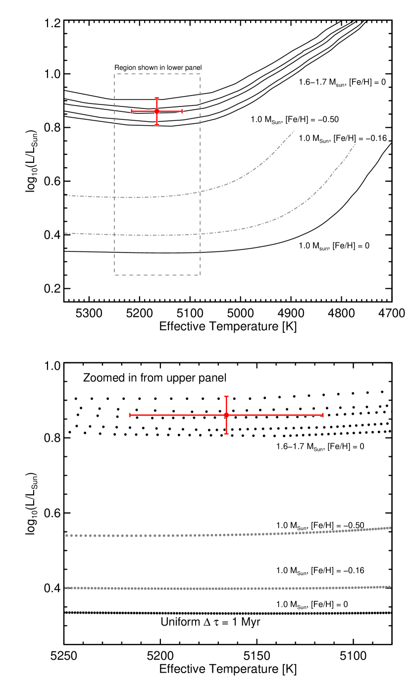
The heart of the problem is that measuring the masses of single stars is necessarily a model-dependent procedure. The most common method of estimating masses is to interpolate theoretical stellar evolution grids at the positions of various measured stellar properties. Typically, the set of parameters used are the stellar effective temperature ($T_{\rm eff}$), luminosity ($L$; or absolute magnitude $\mathcal{M}_{\rm V}$) and metallicity ([Fe/H]) based on LTE atmospheric models fitted to high-resolution stellar spectra (e.g. Valenti & Fischer, 2005; Takeda et al., 2008). The top panel of Figure 1 illustrates a simplified interpolation in which measurements of $T_{\rm eff}$ and $L$ at a fixed [Fe/H] $=0$ (red circle and error bars) are compared to mass tracks from the Yale Rotational Evolution Code models (YREC; Takeda et al., 2007; Demarque et al., 2008, solid black lines). We also demonstrate the effect of metallicity by showing two solar-mass tracks with [Fe/H] $=\{-0.16,-0.50\}$; metallicity acts as a third dimension. At a fixed mass, metal-poor stars are hotter than Solar-metallicity stars, while metal-rich stars are cooler.

Figure 1.— An illustration of the interpolation of model-grids at the position of a subgiant’s spectroscopically-measured $T_{\rm eff}$ and $L$. Top: The subgiant branch of the theoretical Hertzsprung-Russell diagram near the base of the red giant branch. The solid lines show the evolutionary paths of stars of various masses. The red circle shows the position of a specific subgiant and the error bars show the 68.2% confidence region of its effective temperature and luminosity. The dot-dashed lines show two other metallicities for the Solar-mass track, which we include to illustrate the effect of metallicity in this plane. The dashed box traces the region shown in the lower panel. Bottom: A zoomed-in region around the subgiant’s measurements, with the mass tracks shown sampled at a uniform time-spacing of $\Delta\tau=1$ Myr, illustrating the different evolution rates for subgiants of various masses.

2.1. A Probabilistic Framework

The probability of a star’s mass, $M$, given its spectroscopic and photometric parameters and the selection criteria of a survey is given by Bayes’ theorem

$$P(M|T_{\rm eff},{\rm[Fe/H]},L,\mathcal{M}_{V},B-V,\mathcal{I})\propto\\ P(T_{\rm eff},{\rm[Fe/H]},\mathcal{M}_{V}~{}|~{}M)\times\\ P(M~{}|~{}\mathcal{M}_{V},B-V,\mathcal{I})$$ (1)

The left-hand side of the proportionality is an expression for the posterior probability distribution of the stellar mass given a spectroscopic estimate of the stellar effective temperature $T_{\rm eff}$, metallicity [Fe/H], and bolometric luminosity $L$. In addition to the spectroscopic and photometric properties, we also have additional information $\mathcal{I}$, which in our analysis is provided by the galactic population models of Girardi et al. (2005). The term $\mathcal{I}$ encodes information about the stellar IMF, stellar evolution models, and the distribution of ages and metallicities as a function of Galactic scale height (see Dawson et al., 2012, for a similar application).

The right-hand side of Eqn. 1 is the product of two probabilities. The first is the likelihood, which relates the probability of measuring the spectroscopic properties of the star given various choices of the stellar mass from stellar evolution models. The second term describes our prior knowledge about the distribution of stellar masses for stars throughout the Galaxy with a given range of photometric properties.

It is common for investigators using model grid interpolations to focus solely on the likelihood term, because the maximization of the likelihood is directly related to the concept of “chi-squared minimization” when the measured parameters are normally distributed. This can be seen by taking the logarithm of the likelihood, $\mathcal{L}$, with normally-distributed measurement uncertainties on the spectroscopic parameters in Eqn. 1

$$\mathcal{L} \equiv\ln{[P(T_{\rm eff},{\rm[Fe/H]},L)]}$$

$$=C-\frac{1}{2}(\chi^{2}_{\rm T_{\rm eff}}+\chi^{2}_{\rm[Fe/H]}+\chi^{2}_{L})$$ (2)

where, e.g.

$$\chi^{2}_{\rm T_{\rm eff}}=\left[\frac{T_{\rm eff}(M)-T_{\rm eff,meas}}{\sigma_{T_{\rm eff}}}\right]^{2}$$ (3)

Minimization of the $\chi^{2}$ terms maximizes the likelihood of the measurements as a function of $M$. However, this least-squares approach neglects prior information about the distribution of stellar masses.

2.2. The Stellar Mass Prior

Figure 2.— A typical mass probability distribution for a 1.7 M_⊙ subgiant based on atmospheric parameters interpolated onto stellar evolution grids is (likelihood; solid red line), and the prior distribution for stars with comparable colors and absolute magnitudes (solid black line). The resulting mass posterior is the product of the likelihood and prior (dashed blue line) and has a mean of 1.65 M_⊙ (blue arrow), which is roughly 3% lower than the initial estimate without a prior (red arrow). The scaling of the distributions does not matter since such factors scale out of the product and do not affect the centroid or symmetry of the final posterior distribution, hence the proportionality in Eqn. 1. We note that introducing an apparent magnitude cut would move the mean of the prior further toward higher stellar masses.

Even though the measurement errors for stellar properties may be symmetrically distributed across several mass tracks, there is not an equal likelihood of a star having masses under each side of the measurements’ probability distribution. This is both because more massive stars are intrinsically rarer due to the IMF, and because stars of different masses evolve at very different rates. The bottom panel of Figure 1 illustrates this difference in evolutionary rates for the YREC models with uniform time sampling ($\Delta\tau=1$ Myr). Because they evolve slower, there are many more grid points for a Solar-mass star on the subgiant branch than there are for more massive subgiants.

The prior mass distribution must accurately reflect the relative numbers of observable stars of various masses. To generate this prior we used the TRILEGAL Galactic stellar population simulation code that incorporates the IMF, stellar evolution, age-metallicity relationship, and photometric system to produce synthetic stellar populations (Girardi et al., 2005). Girardi et al. present extensive tests of their simulated stellar populations, and demonstrate that they can faithfully reproduce the local H–R diagram and star counts of the Hipparcos and 2MASS catalogs.

We accessed the code using Perl scripts provided by L. Girardi (2012, private communication), with the default Galactic population parameters of the online TRILEGAL 1.5 input form. Specifically, we assumed the Chabrier (2003) IMF, the empirical age-metallicity relationship measured by Rocha-Pinto et al. (2000), and the Padova stellar evolution grids (Girardi et al., 2002). The simulation code also assumes a multi-component Galactic stellar population, with separate prescriptions for the thin/thick disk, bulge and halo. However, our simulated sample of subgiants only extends to $\approx 200$ pc, and therefore only samples the immediate Solar neighborhood.

Given a particular star of interest, one can query the simulation to determine the expected distribution of masses at a given set of observed photometric properties. In our case we use the $B-V$ color and absolute magnitude ($\mathcal{M}_{\rm V}$) since these properties are available from the Hipparcos catalog for all subgiants in the Johnson et al. (2010a) target sample (van Leeuwen, 2007).

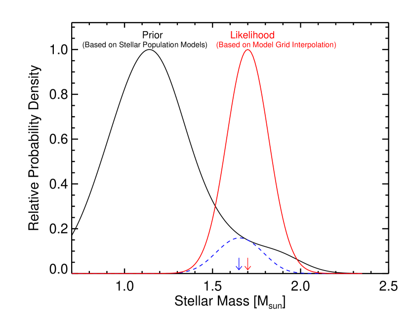
In Figure 2 we illustrate the effect of incorporating such a prior into the mass measurement for a particular subgiant. We consider a star with $B-V=1.00\pm 0.02$ and $\mathcal{M}_{\rm V}$ $=2.2\pm 0.5$. The corresponding stellar mass is $M=1.7\pm 0.12$ M_⊙ based on spectroscopy alone, which represents the likelihood term. We construct the prior using all stars from the TRILEGAL simulations with similar photometric properties, using a 1-$\sigma$ cut in $\mathcal{M}_{\rm V}$ and 3-$\sigma$ cut in $B-V$, to allow for enough stars in the simulation. We find that while this prior distribution peaks at 1.15 M_⊙  the posterior distribution resulting from the product of the likelihood and prior peaks at 1.65 M_⊙. Including the prior, which contains information about the IMF and different evolution rates, results in a mass estimate that is 3% lower than the likelihood alone. Thus, the different evolution rates of subgiants of various masses is not enough to lead to systematically overestimate any individual subgiant’s mass by $\approx 50$%, as suggested by L11.

Note that the prior distribution peaks near 1 M_⊙, similar to the simulated mass distribution of L11. This is because the prior contains no information about the star’s actual metallicity. Once a spectroscopic assessment of the star’s metallicity (and $T_{\rm eff}$) is made, the likelihood function modifies the prior accordingly. That, combined with the high precision of the spectroscopic parameters results in a likelihood term that dominates over the prior and favors higher masses.

3. The Mass Distribution of Subgiants in the Keck Doppler Survey

We next turn our attention to the question of whether these massive subgiants should exist at all. L11 claimed that massive, evolved stars with $M\gtrsim 1.5$ M_⊙ should be exceedingly rare. So much so that the relative numbers of subgiants with masses in excess of 1.5 M_⊙ compared to 1.0-1.2 M_⊙ should be taken as evidence that the inferred masses must be incorrect. To test this hypothesis, we assess the expected distribution of masses for stars selected in the same manner as the targets of Johnson et al. (2010b). As we will show, accounting for all selection criteria is key to properly estimating the expected mass distribution of sample of subgiants.

L11 simulated stellar populations using the YREC stellar evolution models together with assumptions about the form of the Galactic initial mass function (IMF). These features effectively imposed a prior in his Monte Carlo simulations as stars were drawn far less frequently for masses greater than 1.5 M_⊙ than those closer to Solar. In his simulations, L11 found that only 11% of his simulated subgiants had $M>1.5$ M_⊙.

3.1. The importance of a magnitude limit

Stellar evolution and the IMF do not have the final say in shaping the distribution of stellar masses for Doppler survey targets. Surveys of subgiants have specific selection criteria that result in stellar samples that are very different from the Galaxy’s stellar population as a whole. For example, the sample of subgiants monitored at Keck Observatory were selected based on $0.8<B-V<1.05$, $1.8<\mathcal{M}_{V}<3.0$, and $V<8.5$ (Johnson et al., 2010b). Another important criterion used to select subgiants is the requirement that the stars have $M>1.3$ M_⊙ when their Hipparcos B-V colors (van Leeuwen, 2007) and absolute V-band magnitudes ($M_{V}$) are interpolated onto the Padova model grids, under the assumption [Fe/H] $=0$ (Johnson et al., 2010b).

A magnitude criterion was not used in the simulations of L11, but it has a profound impact on the expected mass distribution of a sample of target stars. Consider two stars, with masses 1.2 M_⊙ and 1.8 M_⊙. The IMF predicts a number of stars scales as $M^{-2.4}$, and the evolution rate across the subgiant branch scales as $M^{-3.1}$. The combined effect is a number of subgiants that scales as $M^{-5.5}$ throughout the Galaxy. Assuming a volume-limited survey, as L11 did, results in the expectation of an order of magnitude more 1.2 M_⊙ subgiants compared to 1.8 M_⊙ subgiants.

Now consider the volume $\mathcal{V}\sim d^{3}$ occupied by a star, defined by a distance, $d\sim L^{1/2}$, out to which a star is brighter than the limiting magnitude of the survey. The luminosity of stars on the subgiant branch near the base of the red giant branch scales as $L\sim M^{2.5}$, based on inspection of the YREC model grids (see also Figure 5 of L11). The volume scales with the stellar mass as $\mathcal{V}\sim d^{3}\sim L^{1.5}\sim M^{4}$. An apparent magnitude cut will increase the number of observable, massive subgiants within a given apparent magnitude range, which partially compensates for the dearth of more massive stars due their shorter evolution timescale and the stellar IMF. Imposing a magnitude limit to the selection of stars will result a factor of two fewer 1.8 M_⊙ subgiants compared to 1.2 M_⊙ subgiants. This is much less severe than the prediction of L11, which presumably adopted volume-limited sample (see § 3.2).

This effect is similar to the Malmquist bias in galaxy surveys, in which the magnitude-limited survey sample will result in an apparent overabundance of massive, luminous galaxies at higher redshifts (Malmquist, 1922). The simple scaling arguments presented here give a rough sense for the relative numbers of stars of various masses within a magnitude-limited survey, but they do not account for all effects that will ultimately shape the mass distribution. For a more thorough analysis we again turn to Galactic population models.

3.2. Simulating the expected mass distribution of subgiants

We estimate the stellar mass prior by first simulating samples of stars over the entire sky with a wide range of apparent magnitudes. We then select subgiants from these simulated samples in the same manner that the retired A stars surveyed by Johnson et al. (2010b), namely $0.8<B-V<1.05$, $1.8<$ $\mathcal{M}_{\rm V}$ $<3$, $V<8.5$ and the restriction that the stars’ colors and absolute magnitudes correspond to $M>1.3$ M_⊙ based on Solar-metallicity stellar models.

We simulated 768 lines of sight, uniformly distributed across the sky using the Hierarchical Equal Area isoLatitude Pixelization (HEALPIX) scheme, with the extinction at infinity calculated by the NASA/IPAC extragalactic database (Schlafly & Finkbeiner, 2011). We avoided the galactic plane ($|b|<4^{\circ}$) because TRILEGAL is known to exhibit discrepancies with observational surveys in the Galactic plane (Girardi et al., 2005), and because of the large number of stars returned by those simulations.

Figure 3 shows the resulting distribution of simulated subgiant masses. For ease of future use, we adopt an analytic form of the distribution; we find the posterior distribution is described well by the expression

$$P(M~{}|~{}\mathcal{I})\approx\frac{1+sz}{\sqrt{2\pi\sigma_{M}^{2}}}\exp{\left(-\frac{z^{2}}{2}\right)}$$ (4)

where

$$z=\frac{\log_{10}(M)-M_{0}}{\sigma_{M}}$$ (5)

and $M_{0}=0.134$ M_⊙, $\sigma_{M}=0.0783$ M_⊙ and the dimensional skew term is $s=-0.253$, for all masses $M>0.7$ M_⊙.

Figure 3.— Simulated sample of stars selected with the same criteria as the subgiants in RV surveys (black histogram). The best-fitting log-normal distribution is also shown (red). For comparison, we have also shown the mass distribution reproduced from Figure 4 of L11 (blue dashed lines), which is based on a volume-limited survey rather than a magnitude-limited survey such as ours.

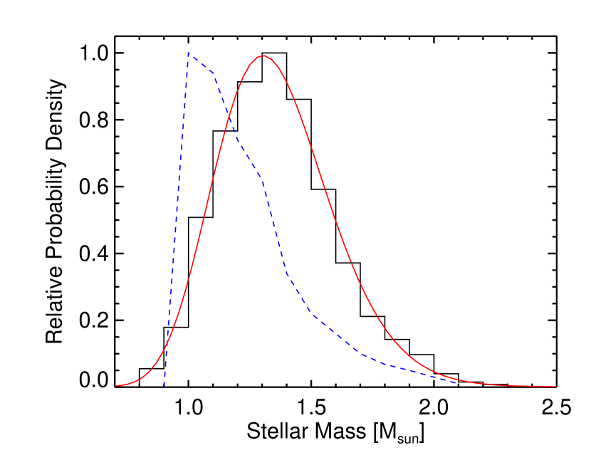
Our stellar mass distribution is qualitatively similar to that shown in Figure 4 of L11. However, while the L11 distribution peaks sharply at 1.0 M_⊙, ours has a peak near 1.3 M_⊙, with relatively few Solar-mass subgiants. Indeed, there are twice as many stars in our simulations with $M>1.5$ M_⊙ as there are for $M<1.1$ M_⊙. The reason for the differences between our simulation and L11’s is the apparent magnitude cut, and the a priori selection of stars that reside near model tracks corresponding to $M>1.3$ M_⊙. While the IMF and subgiant evolution rate favor less massive stars, the higher luminosities of more massive subgiants makes them visible within a much larger volume.

To test the effects of our added selection criteria compared to L11, we selected stars by relaxing certain cuts. By relaxing the criterion $M>1.3$ M_⊙ when stars’ $\mathcal{M}_{\rm V}$ and $B-V$ colors are compared to Solar-metallicity model grids, we find that the low-mass tail of the distribution is filled in, which brings the peak of the posterior distribution down to 1.2 M_⊙. When we impose a volume limit, we recover a distribution very similar to the volume-limited sample shown in Figure 4 of L11.

4. Conclusions

L11 argued that the mass measurements of subgiants with $M>1.5$ M_⊙, i.e. the retired A stars surveyed by Johnson et al. (2010b), must be in error because stars in this mass range should be exceedingly rare. L11 further argues that stellar evolutionary models are sufficiently ambiguous in their predictions (given reasonable uncertainties in their input physics) and that spectroscopically determined stellar parameters are subject to large systematic errors. L11 concludes that the true masses of the stars in the Johnson et al. sample are more reasonably estimated to be 1.0-1.2 solar masses, not typically closer to 1.5 solar masses.

We applied the survey selection criteria of Johnson et al. to the TRILEGAL galactic synthesis models and have shown that the resulting simulated target sample has a mass distribution consistent with the Johnson et al. mass measurements and inconsistent with the prediction of L11. L11 may be correct that stellar evolution and Galactic synthesis models have substantial uncertainties. However, since the TRILEGAL models successfully and accurately reproduces the stellar characteristics of stars in the Solar Neighborhood (Girardi et al., 2005), we find no reason to doubt their accuracy at the level that would implicate the Johnson et al. mass measurements.

Nevertheless, tests of systematic errors in stellar evolution models using planet transit light curves, eclipsing binaries and asteroseismology are very much worthwhile. Fortunately, the large number of transiting planets and eclipsing binaries in the NASA Kepler mission target field (Prša et al., 2011), together with the exquisite photometric precision produced by the Kepler space telescope, will provide many opportunities for these tests in the near future.

References

- Bouchy et al. (2005) Bouchy, F., et al. 2005, A&A, 444, L15
- Chabrier (2003) Chabrier, G. 2003, PASP, 115, 763
- Dawson et al. (2012) Dawson, R. I., et al. 2012, ArXiv e-prints
- Demarque et al. (2008) Demarque, P., et al. 2008, Ap&SS, 316, 31
- do Nascimento et al. (2000) do Nascimento, J. D., et al. 2000, A&A, 357, 931
- Fischer et al. (2005) Fischer, D. A., et al. 2005, ApJ, 620, 481
- Fischer et al. (2003) Fischer, D. A., et al. 2003, ApJ, 586, 1394
- Fischer & Valenti (2005) Fischer, D. A. & Valenti, J. 2005, ApJ, 622, 1102
- Galland et al. (2005) Galland, F., et al. 2005, A&A, 443, 337
- Girardi et al. (2002) Girardi, L., et al. 2002, A&A, 391, 195
- Girardi et al. (2005) Girardi, L., et al. 2005, A&A, 436, 895
- Gray & Nagar (1985) Gray, D. F. & Nagar, P. 1985, ApJ, 298, 756
- Hatzes et al. (2003) Hatzes, A. P., et al. 2003, ApJ, 599, 1383
- Ida & Lin (2004) Ida, S. & Lin, D. N. C. 2004, ApJ, 604, 388
- Johnson et al. (2010a) Johnson, J. A., et al. 2010a, PASP, 122, 905
- Johnson & Apps (2009) Johnson, J. A. & Apps, K. 2009, ApJ, 699, 933
- Johnson et al. (2007a) Johnson, J. A., et al. 2007a, ApJ, 670, 833
- Johnson et al. (2007b) Johnson, J. A., et al. 2007b, ApJ, 665, 785
- Johnson et al. (2010b) Johnson, J. A., et al. 2010b, PASP, 122, 701
- Johnson et al. (2010c) Johnson, J. A., et al. 2010c, PASP, 122, 149
- Lloyd (2011) Lloyd, J. P. 2011, ApJ, 739, L49
- Lovis & Mayor (2007) Lovis, C. & Mayor, M. 2007, A&A, 472, 657
- Malmquist (1922) Malmquist, K. 1922, On Some Relations in Stellar Statistics, Arkiv för matematik, astronomi och fysik (Almqvist & Wiksells)
- Malmquist & Hufnagel (1933) Malmquist, K. G. & Hufnagel, L. 1933, Stockholms Observatoriums Annaler, 11, 9
- Prša et al. (2011) Prša, A., et al. 2011, AJ, 141, 83
- Rocha-Pinto et al. (2000) Rocha-Pinto, H. J., et al. 2000, A&A, 358, 850
- Santos et al. (2004) Santos, N. C., Israelian, G., & Mayor, M. 2004, A&A, 415, 1153
- Sato et al. (2005) Sato, B., et al. 2005, ApJ, 633, 465
- Sato et al. (2007) Sato, B., et al. 2007, ApJ, 661, 527
- Schlafly & Finkbeiner (2011) Schlafly, E. F. & Finkbeiner, D. P. 2011, ApJ, 737, 103
- Takeda et al. (2007) Takeda, G., et al. 2007, ApJS, 168, 297
- Takeda et al. (2008) Takeda, Y., Sato, B., & Murata, D. 2008, PASJ, 60, 781
- Valenti & Fischer (2005) Valenti, J. A. & Fischer, D. A. 2005, ApJS, 159, 141
- van Leeuwen (2007) van Leeuwen, F. 2007, A&A, 474, 653